Nature of long range order in stripe forming systems with long range repulsive interactions

Abstract

We study two dimensional stripe forming systems with competing repulsive interactions decaying as $r^{-\alpha}$. We derive an effective Hamiltonian with a short range part and a generalized dipolar interaction which depends on the exponent $\alpha$. An approximate map of this model to a known XY model with dipolar interactions allows us to conclude that, for $\alpha<2$ long range orientational order of stripes can exist in two dimensions, and establish the universality class of the models. When $\alpha\geq 2$ no long-range order is possible, but a phase transition in the KT universality class is still present. These two different critical scenarios should be observed in experimentally relevant two dimensional systems like electronic liquids ($\alpha=1$) and dipolar magnetic films ($\alpha=3$). Results from Langevin simulations of Coulomb and dipolar systems give support to the theoretical results.

Two dimensional isotropic systems in which a short range attractive interaction competes with a repulsive interaction decaying as a power law of the form $r^{-\alpha}$ have been widely studied Seul and Andelman (1995); Deutsch and Safran (1996); Nussinov et al. (1999); Grousson et al. (2000); Muratov (2002); Ortix et al. (2009); Portmann et al. (2010); Barci et al. (2013a). These include, as physically relevant examples, the dipolar $(r^{-3})$ and the Coulomb $(r^{-1})$ interaction as the repulsive part of the total energy of the system. Dipolar interactions competing with exchange and uniaxial anisotropy arise, e.g. in ultra-thin ferromagnetic films with perpendicular anisotropy Vaterlaus et al. (2000); Wu et al. (2004); Abu-Libdeh and Venus (2009) while long range Coulomb interactions appear in low dimensional electron systems and may be relevant to understand the low temperature phase behavior of doped Mott insulators, two dimensional quantum Hall systems and high $T_{c}$ superconductors Fradkin and Kivelson (1999); Han et al. (2001); Borzi et al. (2007); Parker et al. (2010). It is well known that under certain conditions of relative strength of interactions and external parameters these systems develop modulated stripe-like structures in two dimensions which break space rotational symmetry, similar to classical liquid-crystal systems, giving rise to smectic, nematic and hexatic phases Abanov et al. (1995); Kivelson et al. (1998); Barci et al. (2013b). This analogy, based on the $180^{\circ}$ rotational symmetry of stripe structures and elongated liquid-crystal molecules, allowed to apply well known results for liquid-crystal systems de Gennes and Prost (1998); Chaikin and Lubensky (1995) to predict the qualitative, and to some extent also quantitative phase behavior of many systems with modulated order parameters. Nevertheless, when it is important to understand the true nature of the thermodynamic phases, the analogy between stripe forming systems and classical liquid-crystals should not be taken at face value. The basic units in liquid-crystals are elongated molecules. A given molecule typically interacts with its near neighbors and due to its elongated form a rotation in $180^{\circ}$ of a single molecule does not alter the energy of the system. On the other hand, the smallest relevant scale of a stripe system is the modulation length. At this scale, a basic cell can be considered as containing a single interface and then it is a dipole of opposite densities with an average linear size equal to the modulation length. It is important to note that such dipoles will not be, in general, elementary electric or magnetic dipoles, their character will depend on the nature of the density order parameter under consideration. Having clarified this point, in principle all realistic low energy configurations of the system can be built from these dipole cells. Clearly, a $180^{\circ}$ rotation of a dipole does change the energy of the system and then cannot be considered a local symmetry. The system is only symmetric under global rotations of $180^{\circ}$. Furthermore, when long range interactions are present, it is well known that the behavior of the systems may be very different from those with only short range interactions, which represent the vast majority of classical liquid-crystal systems. A study of the nature of low temperature phases of stripe forming systems should take these elements into account.

Consider a coarse grain Hamiltonian in two dimensions of the form

$$\mathcal{H}[\phi(\vec{x})] = \frac{1}{2}\int d^{2}x\,\left(\vec{\nabla}\phi(\vec{x})\right)^{2}$$ (1)

$$+ \frac{1}{2}\int d^{2}x\int d^{2}x^{\prime}\ \phi(\vec{x}){J}(\vec{x}-\vec{x^{\prime}})\phi(\vec{x^{\prime}})$$

$$+ \frac{1}{2\beta}\int d^{2}x\ V(\phi(\vec{x})),$$

where $\beta=1/k_{B}T$ and $V(\phi)=-\frac{r}{2}\phi^{2}+\frac{u}{4}\phi^{4}$ is a local potential that could be seen as an entropic contribution and which exact form is not important to our work. The long range repulsive interaction has the form $J(\vec{x})=J/|\vec{x}|^{\alpha}$ which allows to analyze in a unified way short range (large $\alpha$) and long range (small $\alpha$) interactions. Physically relevant examples are the Coulomb interaction ($\alpha=1$) and the dipolar interaction between out-of-plane magnetic moments ($\alpha=3$). It is well known that at low temperatures this kind of systems display stripe-like patterns in the form of spatial modulations of the density $\phi(\vec{x})$ Brazovskii (1975); Toner and Nelson (1981); Seul and Andelman (1995); Barci and Stariolo (2007) in a direction represented by a wave vector $\vec{k}_{0}$. Low energy excitations of the stripes can be described in terms of a displacement field $u(\vec{x})$ in the form $\phi(\vec{x})=\sum_{n}\phi_{n}\cos(nk_{0}x+nk_{0}u(\vec{x}))$, where $x$ is the average direction of the modulation and $k_{0}$ stands for the modulus of $\vec{k}_{0}$. If $u(\vec{x})$ varies smoothly in space it is possible to define a local wave vector $\vec{k}_{0}+k_{0}\vec{\nabla}u(\vec{x})$.

The effective Hamiltonian (1) when expressed in terms of $u(\vec{x})$ has local and non-local parts $\mathcal{H}=\mathcal{H}_{l}+\mathcal{H}_{nl}$ (see Supplemental Material). Expanding the local component to quadratic order in the fluctuation field $u$, it can be written in Fourier space as Sornette (1987); de Gennes and Prost (1998); Toner and Nelson (1981):

$$\mathcal{H}_{l}=\mathcal{H}_{0l}+\frac{1}{2}\int\frac{d^{2}k}{(2\pi)^{2}}(\gamma_{x}k_{x}^{2}+\gamma_{y}k_{y}^{4})\hat{u}(\vec{k})\hat{u}(-\vec{k})$$ (2)

where $\gamma_{x}$ and $\gamma_{y}$ are elastic coefficients which are simply related to the parameters of the original Hamiltonian and $\mathcal{H}_{0l}$ represents the local contribution to the energy for an unperturbed stripe. It is well known that this form for the local fluctuations of the stripe pattern leads to a divergence of the mean square of the displacement field, implying the abscence of long range positional order in the system. This is the standard situation in liquid-crystalline systems. We go on to consider the effect of the tail of the long range interaction in the fluctuation spectrum. The non-local component can be taken into account properly by considering the long range interaction between a pair of stripe dipoles as shown schematically in Figure 1.

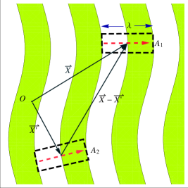
Figure 1: Schematic representation of the long range interaction between two elementary stripe dipoles.

The interaction between a pair of dipoles is given by:

$$\delta\mathcal{H}_{nl}=\frac{J}{2}\int_{\delta A_{1}}d^{2}x\int_{\delta A_{2}}d^{2}x^{\prime}\ \frac{\phi(\vec{x})\phi(\vec{x^{\prime}})}{|\vec{x}-\vec{x^{\prime}}|^{\alpha}}$$ (3)

where $\delta A_{1}$ and $\delta A_{2}$ are the corresponding areas (see Figure 1). If $\lambda$ is the modulation length of the stripe pattern, in the limit $|\vec{x}-\vec{x}^{\prime}|\gg\lambda$ a multipolar expansion of the interaction (3) leads to (see Supplemental Material):

$$\mathcal{H}_{nl} = \frac{1}{2}\gamma\int d^{2}x\int d^{2}x^{\prime}\Omega(|\vec{x}-\vec{x}^{\prime}|)\left(\frac{\vec{e}(\vec{x})\cdot\vec{e}(\vec{x}^{\prime})}{|\vec{x}-\vec{x}^{\prime}|^{\alpha+2}}\right.$$ (4)

$$- \left.(\alpha+2)\frac{\vec{e}(\vec{x})\cdot(\vec{x}-\vec{x}^{\prime})\vec{e}(\vec{x}^{\prime})\cdot(\vec{x}-\vec{x}^{\prime})}{|\vec{x}-\vec{x}^{\prime}|^{\alpha+4}}\right).$$

In this expression $\gamma=\alpha J{P^{2}}$ and $P=\frac{1}{\lambda}\int_{\lambda}dxx\phi(x)$ is the modulus of the dipolar moment. The unit vectors $\vec{e}(\vec{x})$ give the orientation of the dipoles which point along the local wave vector of the stripe pattern and $\Omega(x)$ is a short range cutoff. Here we have neglected fluctuations in the modulation length and accordingly the elastic coefficient $\gamma$ is evaluated in its mean field value (see Supplemental Material for a discussion on relevant fluctuations). As we can see from the expression obtained, the long range repulsive interaction is responsible for a generalized dipolar contribution to the total energy.

Considering again small fluctuations in the direction of the wave vector $\vec{k}_{0}$, we can write $\vec{e}(\vec{x})\approx\frac{\vec{k}_{0}}{k_{0}}+\vec{\nabla}u(\vec{x})$, which leads (considering that $\vec{k}_{0}$ points in $x$ direction) to:

$$\Delta\mathcal{H}_{nl} = \frac{1}{2}\gamma\int d^{2}x\int d^{2}x^{\prime}\Omega(|\vec{x}-\vec{x}^{\prime}|)\left(\frac{\partial_{y}u(\vec{x})\partial_{y^{\prime}}u(\vec{x}^{\prime})}{|\vec{x}-\vec{x}^{\prime}|^{\alpha+2}}\right.$$ (5)

$$- \left.(\alpha+2)\frac{(y-y^{\prime})^{2}\partial_{y}u(\vec{x})\partial_{y^{\prime}}u(\vec{x}^{\prime})}{|\vec{x}-\vec{x}^{\prime}|^{\alpha+4}}\right).$$

Thus, the effective Hamiltonian for the displacement field $u(\vec{x})$ results:

$$\Delta\mathcal{H}=\frac{1}{2}\int\frac{d^{2}k}{(2\pi)^{2}}(\gamma_{x}k_{x}^{2}+\gamma_{y}k_{y}^{4}+\gamma_{nl}k^{\alpha-2}{k_{y}}^{4})\hat{u}(\vec{k})\hat{u}(-\vec{k})$$ (6)

where $\gamma_{nl}=\gamma\alpha(2+\alpha)^{2}C(\alpha+4)$ and the function $C(\alpha)=2^{2-\alpha}{\Gamma(\frac{2-\alpha}{2})}/{\Gamma(\frac{\alpha}{2})}$ with $\Gamma(x)$ being the Gamma function. From the previous considerations we are now in a position to analyze the stability of positional and orientational order of the stripe structures when the long range interactions are taken into account.

Positional order: From the effective Hamiltonian (6) we can see that for $\alpha\geq 2$ the $\gamma_{y}k_{y}^{4}$ term dominates over $\gamma_{nl}k^{\alpha-2}{k_{y}}^{4}$ in the long wavelength limit, i.e. for sufficiently short range interaction no positional order is possible. If $\alpha<2$ the term $\gamma_{nl}k^{\alpha-2}{k_{y}}^{4}$ dominates over $\gamma_{y}k_{y}^{4}$, but even in this longe range interacting regime it is easy to check that the average square fluctuations $\langle u^{2}\rangle=k_{B}T\int\frac{d^{2}k}{(2\pi)^{2}}\left(\gamma_{x}k_{x}^{2}+\gamma_{y}k_{y}^{4}+\gamma_{nl}k^{\alpha-2}{k_{y}}^{4}\right)^{-1}$ diverge with some power of the system size for any $\alpha>0$.

Orientational order: It is well known that in systems with short range interactions orientational order can be weakened by the presence of topological defects  Kosterlitz and Thouless (1973); Toner and Nelson (1981). The typical situation in two dimensional systems with continuous symmetries is that only quasi-long range order is possible when interactions are of sufficiently short range Mermin and Wagner (1966). Nevertheless it is commonly argued that even in systems with long range interactions, like Coulomb or dipolar interactions, shielding effects make the effective interactions short ranged. Here we revisit this question, considering explicitly the effects of the range of the interactions and show that, although the shielding occurs, the effective interactions are still capable of stabilizing a long-range-ordered nematic phase in two dimensions for long enough interaction range.

At low temperatures the stripe structure can be thought of as composed by a mosaic of domains of average size $\xi_{u}$ corresponding to the correlation length of the displacement field $u(\vec{x})$. The orientation of each domain is a natural order parameter which can be described by a unit vector $\vec{n}$. This vector represents the mean orientation of the elementary dipoles inside a domain and consequently it is defined in terms of the unit vectors $\vec{e}(\vec{x})$ previously defined in (4) as :

$$\vec{n}(\vec{x})=\frac{\int_{\Delta A_{u}}d^{2}x\,\vec{e}(\vec{x})}{\left|\int_{\Delta A_{u}}d^{2}x\,\vec{e}(\vec{x})\right|},$$ (7)

where $\Delta A_{u}$ is the area of the domain, and it is over this area that a coarse graining process is made. Proceeding as in the analysis of positional order, we can separate the contribution to the orientational energy into two parts, a local part coming from interactions between nearby domains and a non-local one due to interactions between far apart domains. In the long wavelength limit, at the scale of the correlation length $\xi_{u}$, the effective interaction between nearby domains will be of the form:

$$\Delta\mathcal{H}_{ol}=\frac{\gamma_{ol}}{2}\int d^{2}x\,(\vec{\nabla}\theta)^{2}(\vec{x})$$ (8)

where $\theta(\vec{x})$ is the angle between two neighboring domains pointing along directions $\vec{n}$ and $\vec{n}^{\prime}$. The elastic coefficient $\gamma_{ol}$ can be estimated to be $J\alpha^{2}P^{2}/(4\xi_{u}^{\alpha-2})$. To continue with our analysis we realize that over length of order $\xi_{u}$, deviations of the local directors $\vec{e}(x)$ are small. This means after a coarse graining process, the interactions between far apart well polarized domains ( of typical size $\xi_{u}\times\xi_{u}$ ) has the same form of Eq. (4):

$$\mathcal{H}_{onl} = \frac{\gamma}{2}\int d^{2}x\int d^{2}x^{\prime}\,\Omega(|\vec{x}-\vec{x}^{\prime}|)\left(\frac{\vec{n}(\vec{x})\cdot\vec{n}(\vec{x}^{\prime})}{|\vec{x}-\vec{x}^{\prime}|^{\alpha+2}}\right.$$ (9)

$$- \left.(\alpha+2)\frac{\vec{n}(\vec{x})\cdot(\vec{x}-\vec{x}^{\prime})\vec{n}(\vec{x}^{\prime})\cdot(\vec{x}-\vec{x}^{\prime})}{|\vec{x}-\vec{x}^{\prime}|^{\alpha+4}}\right)$$

as a consequence of the principle of superposition. Then, $\mathcal{H}_{o}=\mathcal{H}_{ol}+\mathcal{H}_{onl}$ is the complete orientational effective Hamiltonian. This is one of the main results of our work (see Supplemental Material). Note that usually the effective orientational energy is taken to be composed only by the local part, corresponding to smooth variations in the mean directions of neighboring striped domains. We will see in the sequel that the presence of the second (non-local) term can potentially change the universality class of the orientational order in the system. A renormalization group study of the orientational effective Hamiltonian $\mathcal{H}_{o}$ has been done before in Ref. Maier and Schwabl, 2004 for the case $\alpha=1$, which corresponds to a dipolar XY model. In that reference, the authors were able to renormalize the model and, importantly, they showed that the universal properties are not changed by the presence of the anisotropic part of the interaction. Furthermore, they showed that a whole family of models with isotropic long range interactions of the form $\int_{\vec{k}}|k|^{\sigma}\vec{S}(\vec{k})\vec{S}(-\vec{k})$ behave in qualitatively the same way as the dipolar XY model as long as the range $\sigma<2$. Once the mapping between these models and ours is established then the critical properties of the stripe forming systems are known. In fact, the Fourier transform of the isotropic term in Eq. (9) is proportional to $\int_{\vec{k}}|k|^{\alpha}\vec{n}(\vec{k})\vec{n}(-\vec{k})$ Barci et al. (2013a). Then, one immediately see that for $\alpha\geq 2$ the leading term in $\mathcal{H}_{o}$ is quadratic in $k$. In this case the low temperature physics of the system is that of the two dimensional short range XY model, i.e. there is a phase transition of the Kosterlitz-Thouless type at a critical temperature $T_{KT}$. In a system with dipolar interactions $\alpha=3$ and then we expect it to have an isotropic-nematic phase transition of the KT type, as anticipated in previous works based on analysis of fluctuations of the local part of the effective Hamiltonian Barci and Stariolo (2007, 2009). In this case nematic order is quasi-long-range with algebraically decaying correlations. However, when $\alpha<2$ the physics changes according to the results of Ref. Maier and Schwabl, 2004. Now, the non-local part in $\mathcal{H}_{o}$ is relevant and rules the low temperature phase transition. In fact, the long range nature of the interactions in this sector are able to stabilize a nematic phase with truly long range order below a critical temperature $T_{c}$. It is possible to show, in the framework of renormalization group equations, that the critical properties of the systems for $\alpha<2$ show some peculiar characteristics, for example Maier and Schwabl (2004):

• in the critical region, the correlation length diverges exponentially at $T_{c}$, from both sides, as $\xi_{o}\propto\exp\left(\frac{b}{\sqrt{|T_{c}-T|}}\right)$, reminiscent of the KT transition behavior.

• For $T<T_{c}$ in the critical region, the average dipolar moment behaves as $M\propto\xi_{o}(T)^{-(2-\alpha)/2}$, showing the existence of long range order when $\alpha<2$.

• The orientational susceptibility diverges as $\chi_{o}\propto\xi_{o}(T)^{\alpha}$ in the critical region.

This kind of behavior should be observable, e.g. in systems with long range Coulomb interactions for which $\alpha=1$. This case maps onto the dipolar XY model analyzed in Maier and Schwabl, 2004 and the results may be relevant to understand the phase behavior of two dimensional electron systems. In the next section we show results from computer simulations of systems with $\alpha=1$ (Coulomb) and $\alpha=3$ (dipolar) which give support to the different scenarios in both systems as described before.

Simulation results: We performed Langevin simulations of the Hamiltonian (1). The relaxational (overdamped) Langevin dynamics of the density $\phi(\vec{x})$ is defined in reciprocal space by:

$$\frac{\partial\phi}{\partial t}(\vec{k},t)=-\mathcal{A_{\alpha}}(k)\phi(\vec{k},t)-u[\phi^{3}]_{F}(\vec{k},t)+\eta(\vec{k},t)$$ (10)

where $\mathcal{A_{\alpha}}(k)$ is the spectrum of fluctuations, i.e. the Fourier transform of the quadratic part of the effective Hamiltonian (1), $[\phi^{3}]_{F}(\vec{k},t)$ stands for the Fourier transform of $\phi^{3}(\vec{x},t)$ and $\eta(\vec{k},t)$ represents a Gaussian white noise with correlations $<\eta(\vec{k},t)\eta(\vec{k}^{\prime},t^{\prime})>=(2\pi)^{2}2T\delta(\vec{k}+\vec{k}^{\prime})\delta(t-t^{\prime})$, where $T$ is the effective temperature of the heat bath. We worked with two forms of $\mathcal{A_{\alpha}}(k)$, the first one $\mathcal{A}_{3}(k)=a_{2}(k-k_{0})^{2}-r$ encodes the linear dependence of the isotropic dipolar interaction with $k$, with $a_{2}$ and $r$ constants. The second form is $\mathcal{A}_{1}(k)=a_{2}(k^{2}+2k_{0}^{3}/k-3k_{0}^{2})-r$, corresponding to the Coulomb interaction proportional to $1/k$ in two dimensional Fourier space. The parameters were chosen such as to have the same values of $\mathcal{A_{\alpha}}(k)$ close to the minimum at $k_{0}$. To ensure this we have set $a_{2}=1$ for the dipolar and $a_{2}=1/3$ for the Coulomb cases. In both cases we set $r=1$ and $k_{0}=1$.

For the numerical simulations we have used an implicit first-order scheme for the numerical integration of (10) in the Fourier space, a procedure that guarantees good numerical stability with time step $dt=0.1$, as established in previous works Nicolao and Stariolo (2007); Díaz-Méndez et al. (2011). In the adimensional form, the periodicity of the stripes are set by the lattice constant $dx$ of a 2d square grid with linear size $L=MN$, so that $\vec{k}=(k_{x}/dx,k_{y}/dx)$ with $k_{i}=2\pi n_{i}/L$ and $dx=\pi/M$. Within this scheme, the stripe length span $M$ lattice sites and the linear system size is such that contains $N$ stripes. We fixed $M=11$ in order to have smooth domain walls.

After an estimation of the equilibration and correlation times from high temperature quenches, we performed slow cooling experiments and found that below $T\simeq 0.59$ ($T\simeq 0.45$) the dipolar (Coulomb) systems find themselves in the low temperature phases (with orientational order) for all system sizes. Above those temperatures the configurations are in a state usually called liquid of stripes, where both positional and orientational correlation lengths are finite. So we concentrated on equilibrium simulations for $T=0.57$ ($T=0.43$) for system sizes ranging from $(12\times 11)^{2}$ up to $(66\times 11)^{2}$. The orientational order was quantified through the local director field $\vec{v}(\vec{x})=\vec{\nabla}\phi(\vec{x})/|\vec{\nabla}\phi(\vec{x})|$ by measuring $Q=\langle\cos{2\theta(\vec{x})}\rangle$ and its corresponding susceptibility $\chi_{o}$, where $\theta(\vec{x})$ is the angle defining the local orientation of the director field.

The previous analysis implies that, in the limit of large system sizes, the orientational susceptibility for interactions with $\alpha=1$ and $\alpha=3$ should be qualitatively different for $T<T_{c}$. In the Coulomb case, the second order nature of the phase transition should imply that the susceptibility must be finite when $N\to\infty$. On the other hand, for dipolar interactions the transition should be of the KT type, implying a monotonic (logarithmic) increase of $\chi_{o}$ with system size, which should diverge in the thermodynamic limit for all $T\leq T_{KT}$. Results for the orientational susceptibility as a function of the linear system size ($N=L/11$) from simulations are shown in Fig. 2 for the two characteristic temperatures cited above, corresponding to the low temperature phase of each model. Although computational limitations prevent us to reach very large system sizes, it is clarly observed that the susceptibility of the Coulomb system ($\alpha=1$) first grows with $N$ but eventually suffers a crossover and then saturates at a fixed value for the largest sizes. On the other hand, the susceptibility in the dipolar system ($\alpha=3$) shows a power law increase with system size, a behavior consistent with that of a KT-like critical phase. Of course, we cannot conclude that $\chi_{o}$ will not saturate at larger $N$’s, but the different trend observed in both systems for equivalent parameter values is a strong indication that the theoretical results are indeed correct.

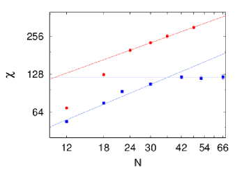
Figure 2: Orientational susceptibility of the Coulomb (blue squares) and dipolar (red dots) models as function of the linear size of the systems in log-log scale. The full lines are power law fits with exponents 0.7 (blue) and 0.6 (red).

In summary, we have shown that two-dimensional stripe forming systems with isotropic competing interactions can be classified into two universality classes: for sufficiently short-range interactions a Kosterlitz-Thouless transition from an isotropic to a quasi-long-range orientational order phase takes place with the well known phenomenology of defect-mediated phase transitions; but, for sufficiently long-range repulsive interactions a second order phase transition with some unusual characteristics drives the system from the isotropic to a fully long-range orientational order phase. These results improve considerably the understanding of the nature of phase transtions in stripe forming systems and may be relevant to a wide variety of systems, particularly the strong correlated regime of two dimensional “electronic liquid-crystals” phases and modulated phases in ultrathin magnetic films with perpendicular anisotropy.

Acknowledgments: We gratefully acknowledge partial financial support from CNPq (Brazil) and the Laboratório de Física Computacional from IF-UFRGS for the use of the cluster Ada.

References

- Seul and Andelman (1995) M. Seul and D. Andelman, Science 267, 476 (1995).
- Deutsch and Safran (1996) A. Deutsch and S. A. Safran, Phys. Rev. E 54, 3906 (1996).
- Nussinov et al. (1999) Z. Nussinov, J. Rudnick, S. A. Kivelson, and L. N. Chayes, Phys. Rev. Lett. 83, 472 (1999).
- Grousson et al. (2000) M. Grousson, G. Tarjus, and P. Viot, Phys. Rev. E 62, 7781 (2000).
- Muratov (2002) C. B. Muratov, Phys. Rev. E 66, 066108 (2002).
- Ortix et al. (2009) C. Ortix, J. Lorenzana, and C. D. Castro, Physica B: Condensed Matter 404, 499 (2009).
- Portmann et al. (2010) O. Portmann, A. Gölzer, N. Saratz, O. V. Billoni, D. Pescia, and A. Vindigni, Phys. Rev. B 82, 184409 (2010).
- Barci et al. (2013a) D. G. Barci, L. Ribeiro, and D. A. Stariolo, Phys. Rev. E 87, 062119 (2013a).
- Vaterlaus et al. (2000) A. Vaterlaus, C. Stamm, U. Maier, M. G. Pini, P. Politi, and D. Pescia, Phys. Rev. Lett. 84, 2247 (2000).
- Wu et al. (2004) Y. Z. Wu, C. Won, A. Scholl, A. Doran, H. W. Zhao, X. F. Jin, and Z. Q. Qiu, Physical Review Letters 93, 117205 (2004).
- Abu-Libdeh and Venus (2009) N. Abu-Libdeh and D. Venus, Phys. Rev. B 80, 184412 (2009).
- Fradkin and Kivelson (1999) E. Fradkin and S. A. Kivelson, Phys. Rev. B 59, 8065 (1999).
- Han et al. (2001) J. Han, Q.-H. Wang, and D.-H. Lee, Int. J. Mod. Phys. B 15, 1117 (2001).
- Borzi et al. (2007) R. A. Borzi, S. A. Grigera, J. Farrell, R. S. Perry, S. J. S. Lister, S. L. Lee, D. A. Tennant, Y. Maeno, and A. P. Mackenzie, Science 315, 214 (2007).
- Parker et al. (2010) C. V. Parker, P. Aynajian, E. H. da Silva Neto, A. Pushp, S. Ono, J. Wen, Z. Xu, G. Gu, and A. Yazdani, Nature 468, 677 (2010).
- Abanov et al. (1995) A. Abanov, V. Kalatsky, V. L. Pokrovsky, and W. M. Saslow, Phys. Rev. B 51, 1023 (1995).
- Kivelson et al. (1998) S. A. Kivelson, E. Fradkin, and V. J. Emery, Nature 393, 550 (1998).
- Barci et al. (2013b) D. G. Barci, A. Mendoza-Coto, and D. A. Stariolo, Phys. Rev. E 88, 062140 (2013b).
- de Gennes and Prost (1998) P. G. de Gennes and J. Prost, The Physics of Liquid Crystals (Oxford University Press, 1998).
- Chaikin and Lubensky (1995) P. M. Chaikin and T. C. Lubensky, Principles of Condensed Matter Physics (Cambridge University Press, 1995).
- Brazovskii (1975) S. A. Brazovskii, Sov. Phys. JETP 41, 85 (1975).
- Toner and Nelson (1981) J. Toner and D. R. Nelson, Phys. Rev. B 23, 316 (1981).
- Barci and Stariolo (2007) D. G. Barci and D. A. Stariolo, Phys. Rev. Lett. 98, 200604 (2007).
- Sornette (1987) D. Sornette, J. Physique 48, 151 (1987).
- Kosterlitz and Thouless (1973) J. M. Kosterlitz and D. J. Thouless, J. Phys. C: Solid State Physics 6, 1181 (1973).
- Mermin and Wagner (1966) N. D. Mermin and H. Wagner, Phys. Rev. Lett. 17, 1133 (1966).
- Maier and Schwabl (2004) P. G. Maier and F. Schwabl, Phys. Rev. B 70, 134430 (2004).
- Barci and Stariolo (2009) D. G. Barci and D. A. Stariolo, Phys. Rev. B 79, 075437 (2009).
- Nicolao and Stariolo (2007) L. Nicolao and D. A. Stariolo, Phys. Rev. B . 76, 054453 (2007).
- Díaz-Méndez et al. (2011) R. Díaz-Méndez, A. Mendoza-Coto, R. Mulet, L. Nicolao, and D. A. Stariolo, Eur. Phys. J. B 81, 309 (2011).