Effect of broadening in the weak coupling limit of vibrationally coupled electron transport through molecular junctions and the analogy to quantum dot circuit QED systems

Abstract

We investigate the nonequilibrium population of a vibrational mode in the steady-state of a biased molecular junction, using a rate equation approach. We focus on the limit of weak electronic-vibrational coupling and show that, in the resonant transport regime and for sufficiently high bias voltages, the level of vibrational excitation increases with decreasing coupling strength, assuming a finite and non-zero value. An analytic behavior with respect to the electronic-vibrational coupling strength is only observed if the influence of environmental degrees of freedom is explicitly taken into account. We consider the influence of three different types of broadening: hybridization with the electrodes, thermal fluctuations and the coupling to a thermal heat bath. Our results apply to vibrationally coupled electron transport through molecular junctions but also to quantum dots coupled to a microwave cavity, where the photon number can be expected to exhibit a similar behavior.

I Introduction

The interplay of electronic degrees of freedom with phonons or photons is relevant for a wide range of condensed matter systems. This includes systems where electrons interact with local vibrational degrees of freedom such as, for example, in molecules, or with delocalized lattice vibrations (phonons) such as, for example, in solids. The interaction of electrons and photons can be understood on similar grounds, identifying the electric field strength with the displacement of a vibrational or a phonon degree of freedom. Thus, for example, matter-light interaction is often described by Hamiltonians Schäfer and Wegener (2002); Delbecq et al. (2011) that are very similar to the ones used to describe electron-phonon interactions Mahan (1981).

The coupling results in mutual excitation and deexcitation processes. For example, phonons or photons can be excited via a deexcitation of the electronic subsystem. Such an excitation decays typically fast, if the phonon or photon field is delocalized and the excitation energy is transferred efficiently away from the place of interaction. This is the situation when the electrons are under the influence of an external electric field or interact with phonons in a solid. The situation is different for nanostructures where the bosonic degrees of freedom are localized. The simplest realization of such a scenario is a molecule. Photons can be localized inside a cavity Raimond et al. (2001); Wallraff et al. (2004); Chiorescu et al. (2004). In both cases, the bosonic degrees of freedom can be driven into highly excited nonequilibrium states Koch et al. (2006a); Härtle et al. (2009); Härtle and Thoss (2011a); Romano et al. (2010); Schiró and Le Hur (2014); Abdullah et al. (2014); Kulkarni et al. (2014); Schinabeck et al. (2014). It is challenging to understand these states, because they cannot be described via a Bose-Einstein distribution function. Nevertheless, these states determine the functionality and efficiency of many devices that may be used for nanoelectronic applications Boese and Schoeller (2001); Cuniberti et al. (2005); Koch and von Oppen (2005); Zazunov et al. (2006); Härtle et al. (2009); Galperin et al. (2009); Leijnse and Wegewijs (2008); Romano et al. (2010); Cuevas and Scheer (2010); Härtle and Thoss (2011a); Wang et al. (2012); Härtle et al. (2013), quantum information processing Skolnick and Mowbray (2004); Cuniberti et al. (2005); Schoelkopf and Girvin (2008); Juska et al. (2013), solar energy conversion Selinsky et al. (2013); Wang et al. (2014); Wu and Wang (2014); Ajisaka et al. (2015) or the control of chemical processes Brumer and Shapiro (2003); Pascual et al. (2003); Härtle et al. (2010); Dzhioev and Kosov (2011); Volkovich et al. (2011).

In this work, we investigate the nonequilibrium properties of a vibrational mode in a single-molecule junction. Thereby, the molecule is contacted by two electrodes which represent macroscopic electron reservoirs. This can be achieved, for example, using a scanning tunneling microscope, electromigration or break-junction techniques Nitzan (2001); Tao (2006); Selzer and Allara (2006); Chen et al. (2007); Cuevas and Scheer (2010). A bias voltage can be applied such that electrons tunnel through the molecule. Due to the small size and mass of a molecule, the tunneling electrons are likely to interact with the molecules vibrational modes, leading to inelastic tunneling processes where vibrational motion is excited and deexcited May (2002); Flensberg (2003); Mitra et al. (2004); Wu et al. (2004); Galperin et al. (2004); Frederiksen et al. (2004); Cizek et al. (2004); Wegewijs and Nowack (2005); Galperin et al. (2007); Avriller and Levy Yeyati (2009); Schmidt and Komnik (2009); Haupt et al. (2009); Härtle et al. (2009); Leijnse and Wegewijs (2008); Koch et al. (2010); Urban et al. (2010); Entin-Wohlman et al. (2010); Esposito and Galperin (2010); Dash et al. (2012); Härtle et al. (2013); Schinabeck et al. (2014). This behavior has been observed in a number of experiments Yu et al. (2004); Kushmerick et al. (2004); Qiu et al. (2004); Sapmaz et al. (2005); Pasupathy et al. (2005); Sapmaz et al. (2006); Thijssen et al. (2006); Parks et al. (2007); Böhler et al. (2007); de Leon et al. (2008); Repp et al. (2010); Hüttel et al. (2009); Hihath et al. (2010); Ballmann et al. (2010). The observation, however, is often indirect, because a direct measurement of the level of vibrational excitation, for example via Raman spectroscopy Ward et al. (2008); Ioffe et al. (2008); Ward et al. (2011), is very involved.

The level of vibrational excitation may be more easily and more reliably accessed in quantum dot systems which are coupled to a microwave cavity (circuit quantum electrodynamics) Yoshie et al. (2004); Reithmaier et al. (2004); Petersson et al. (2011); Delbecq et al. (2011, 2013); Liu et al. (2014). Here, the quantum dots take on a similar role as the molecule in a molecular junction, while the number of photons inside the cavity correspond to the excitation number of a local vibrational mode. Infact, measurements of the photon number have been reported recently Viennot et al. (2014). Identifying again the electric field strength with the displacement coordinate of a vibrational mode, the theoretical description of these systems is very similar Delbecq et al. (2011, 2013); Schiró and Le Hur (2014); Abdullah et al. (2014); Kulkarni et al. (2014); Cottet et al. (2015) (cf. Fig. 1). In contrast to single-molecule junctions, however, where the contact geometry and other (e.g. internal) coupling parameters are hard to control, experiments on quantum dot systems can be carried out with greater precision and more handles of control, including, for example, the wide tunability of the electron-photon coupling strength Delbecq et al. (2013); Viennot et al. (2014). Given these remarkable analogies, vibrational dynamics in a molecular junction can be used to understand quantum impurity circuit-QED systems and vice versa.

In this contribution, we focus on the counterintuitive prediction that, in a molecular junction at sufficiently high bias voltages, the level of vibrational excitation increases with decreasing electronic-vibrational coupling strengths. This phenomenon has been reported in a number of theoretical studies Mitra et al. (2004); Koch et al. (2006a); Avriller (2011); Härtle and Thoss (2011b); Kast et al. (2011) and explained via the suppression of electron-hole pair creation processes Härtle and Thoss (2011b). The latter study was based on Born-Markov theory and pointed out the connection between the limits of an infinite bias voltage and a vanishing electronic-vibrational coupling strength. Thereby, the hybridization of the junctions levels with the electrodes, thermal broadening and the effect of a heat bath has been discarded. We take a big step forward and extend these considerations by broadening effects, verifying that the slope of the vibrational excitation level as function of electronic-vibrational coupling can be negative over a wide range of parameters. Due to broadening, the level of vibrational excitation stays finite in the limit of a vanishing coupling and does not increase indefinitely as the coupling constant vanishes. Moreover, we show that the non-analytic behavior is an artifact of the model itself. For non-zero coupling strengths and/or in presence of a heat bath (analogous to the leakage of photons in the cavity context) we find an analytic behavior. While the electronic-vibrational coupling is hard to control in molecular junctions, quantum dot realizations may give a direct access to this phenomenon, that is a decrease of the level of vibrational excitation or photon number with an increasing coupling strength.

The article is organized as follows. In Sec. II, we outline the theoretical methodology. This includes our model of a molecular junction (Sec. II.1) and the Born-Markov theory that we use to solve this transport problem (Secs. II.2). In addition, we outline an extension of the approach by higher order processes, which involves off-resonant pair creation processes and cotunneling in terms of transition rates (Sec. II.3). Our results are presented in Sec. III. We first review the basics of the phenomenon (Sec. III.1) and continue to discuss the effect of broadening on the level of vibrational excitation in the limit of vanishing electronic-vibrational coupling (Sec. III.2). The next section (Sec. III.3) is devoted to the effect of excitation and deexcitation processes due to inelastic cotunneling Koch et al. (2006b); Lüffe et al. (2008) and off-resonant electron-hole pair creation processes Volkovich et al. (2011). We show that these effects can only be properly accounted for if broadening effects are considered, while, otherwise, these processes have no impact on our phenomenon of interest. In Sec. III.4, we will finally address broadening of the vibrational levels due to coupling to a heat bath.

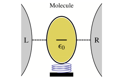
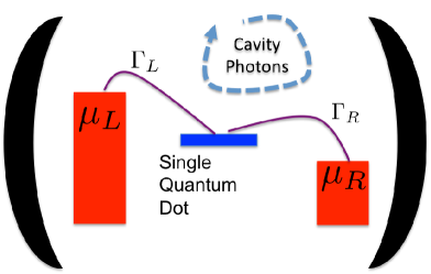
Figure 1: Schematic figure of a single-molecule junction (left) and a single quantum dot circuit-QED setup (right). The coupling between a local vibrational mode of the molecule, which is depicted by a spring, to one of the molecular electronic levels can be described in the same Holstein-like way as the coupling between the microwave photons of a cavity and the electronic levels of a quantum dot inside the cavity.

II Theory

II.1 Model hamiltonian

We consider vibrationally coupled electron transport through a nanostructure that can be represented by a single electronic state. The Hamiltonian of this transport scenario can be written as follows (using units where $\hbar=1$)

$$H = \epsilon_{0}d^{\dagger}d+\sum_{k\in\text{L,R}}\epsilon_{k}c_{k}^{\dagger}c_{k}+\sum_{k\in\text{L,R}}(V_{k}c^{\dagger}_{k}d+\text{h.c.})+\Omega a^{\dagger}a+\lambda(a+a^{\dagger})d^{\dagger}d$$

$$+\sum_{\beta}\omega_{\beta}b_{\beta}^{\dagger}b_{\beta}+\sum_{\beta}\eta_{\beta}(a+a^{\dagger})(b_{\beta}+b_{\beta}^{\dagger})$$

Here, $\epsilon_{0}$ denotes the energy of the electronic state. It is coupled to electronic states with energies $\epsilon_{k}$ that are located in the left (L) and the right (R) electrode. The corresponding coupling matrix elements are given by $V_{k}$. Each of these states is addressed by creation/annihilation operators $d^{\dagger}$/$d$ and $c_{k}^{\dagger}/c_{k}$, respectively. For the vibrational degrees of freedom, we employ a simplified picture, where we use a single harmonic mode with frequency $\Omega$. The corresponding creation and annihilation operators are $a^{\dagger}$ and $a$. The coupling strength between the harmonic mode and the electronic state is denoted by $\lambda$. In addition, we consider a direct coupling of the local vibrational degree of freedom to a bath of oscillators Weiss (1993); Thoss and Domcke (1998); Härtle et al. (2008, 2010). They are addressed by the creation and annihilation operators $b_{\beta}^{\dagger}$ and $b_{\beta}$. The corresponding coupling strengths are given by $\eta_{\beta}$. Thus, we account for a coupling of the local vibrational mode to the phonon modes in the electrodes Jorn and Seidemann (2009), other environmental degrees of freedom, such as, e.g., in an electrochemically gated molecular junction Tao (2006) and/or intramolecular vibrational energy redistribution Mukamel and Smalley (1980); Freed and Nitzan (1983); Zewail (1994); Nesbitt and Field (1996). In the quantum dot circuit QED context, these terms simulate the leakage of photons out of the cavity.

Using the small polaron transformation Mitra et al. (2004), which, in the presence of a heat bath, can be carried out iteratively as long as $4\sum_{\beta}\frac{\left|\eta_{\beta}\right|^{2}}{\Omega\omega_{\beta}}<1$ Galperin et al. (2006); Härtle et al. (2008, 2009), the Hamiltonian $H$ can be pre-diagonalized. The transformed Hamiltonian $H\rightarrow\overline{H}$ is given by

$$\overline{H} = \overline{H}_{\text{S}}+\overline{H}_{\text{L+R+bath}}+\overline{H}_{\text{SL+SR+Sbath}},$$ (2)

$$\overline{H}_{\text{S}} = \overline{\epsilon}_{0}d^{\dagger}d+\Omega a^{\dagger}a,$$ (3)

$$\overline{H}_{\text{L+R+bath}} = \sum_{k}\epsilon_{k}c_{k}^{\dagger}c_{k}+\sum_{\beta}\omega_{\beta}b_{\beta}^{\dagger}b_{\beta},$$ (4)

$$\overline{H}_{\text{SL+SR+Sbath}} = \sum_{k}(V_{k}Xc_{k}^{\dagger}d+\text{h.c.})+\sum_{\beta}\eta_{\beta}(a+a^{\dagger})(b_{\beta}+b_{\beta}^{\dagger}).$$ (5)

It involves a system (S) Hamiltonian, $\overline{H}_{\text{S}}$, which comprises the polaron-shifted electronic level, $\overline{\epsilon}_{0}=\epsilon_{0}-\lambda^{2}/\Omega$, and the harmonic mode. The leads degrees of freedom and the heat bath are included in $\overline{H}_{\text{L+R+bath}}$. The term $\overline{H}_{\text{SL+SR+Sbath}}$ describes the coupling between the electronic state and the leads and between the local vibrational mode and the heat bath. As a result of the polaron transformation, there is no direct electronic-vibrational coupling term in $\overline{H}_{\text{S}}$, but the coupling matrix elements $V_{k}$ become dressed by the shift operator $X=\text{exp}((\lambda/\Omega)(a-a^{\dagger}))$. Throughout this work, we assume the wide-band approximation where the level-width function

$$\Gamma_{K}(\epsilon) = 2\pi\sum_{k\in K}|V_{k}|^{2}\delta(\epsilon-\epsilon_{k})$$ (6)

is approximated by a constant $\Gamma_{K}(\epsilon)=\Gamma_{K}$ ($K\in\{\text{L,R}\}$). Moreover, we characterize the effect of the heat bath via the constant dissipation rate

$$\gamma_{\text{bath}} = 2\pi\sum_{\beta}|\eta_{\beta}|^{2}\delta(\Omega-\omega_{\beta}).$$ (7)

Note that, here and in the following, we neglected any renormalization effects due to the coupling to the thermal heat bath and assume $\sum_{\beta}\frac{\left|\eta_{\beta}\right|^{2}}{\Omega\omega_{\beta}}\ll 1$.

II.2 Born-Markov master equation approach

We address the transport problem, which is described by the Hamiltonian $\overline{H}$, employing Born-Markov theory. The corresponding master equation is well established May (2002); Mitra et al. (2004); Lehmann et al. (2004); Harbola et al. (2006); Volkovich et al. (2008); Härtle et al. (2009); Härtle and Thoss (2011a). The central quantity of this theory is the reduced density matrix $\sigma$. It is determined by the equation of motion

$$\frac{\partial\sigma(t)}{\partial t} = -i\left[\overline{H}_{\text{S}},\sigma(t)\right]$$

$$-\int_{0}^{\infty}\text{d}\tau\,\text{tr}_{\text{L+R+bath}}\{\left[\overline{H}_{\text{SL+SR+Sbath}},\left[\overline{H}_{\text{SL+SR+Sbath}}(\tau),\sigma(t)\sigma_{\text{L}}\sigma_{\text{R}}\sigma_{\text{bath}}\right]\right]\},$$

where

$$\overline{H}_{\text{SL+SR+Sbath}}(\tau) = \text{e}^{-i(\overline{H}_{\text{S}}+\overline{H}_{\text{L+R+bath}})\tau}\overline{H}_{\text{SL+SR+Sbath}}\text{e}^{i(\overline{H}_{\text{S}}+\overline{H}_{\text{L+R+bath}})\tau}$$ (9)

and $\sigma_{K}$ and $\sigma_{\text{bath}}$ represent the equilibrium density matrix of lead $K$ and the heat bath, respectively. This equation of motion constitutes a second-order expansion of the Nakajima-Zwanzig equation Nakajima (1958); Zwanzig (1960) with respect to the coupling term $\overline{H}_{\text{SL+SR+Sbath}}$, where, in addition, the so-called Markov approximation is employed.

We evaluate the master equation (II.2) with the product basis $|0\rangle|\nu\rangle$ and $|1\rangle|\nu\rangle$, which refers to the $\nu$th level of the harmonic mode ($\nu\in\mathbb{N}_{0}$) and the unoccupied $|0\rangle$ and occupied electronic level $|1\rangle$, respectively. In the following, we consider only the diagonal elements of the reduced density matrix, because the respective off-diagonal elements do not play a role in what follows (cf. the discussion in the appendix of Ref. Härtle and Thoss (2011a)). The diagonal elements can be written as

$$\sigma_{0}^{\nu}\equiv\langle 0|\sigma^{\nu}|0\rangle\equiv\langle 0|\langle\nu|\sigma|\nu\rangle|0\rangle,$$ (10)

$$\sigma_{1}^{\nu}\equiv\langle 1|\sigma^{\nu}|1\rangle\equiv\langle 1|\langle\nu|\sigma|\nu\rangle|1\rangle.$$ (11)

In the steady state regime, where $\partial_{t}\sigma=0$, the master equation (II.2) thus reduces to the rate equations

$$0 = -\sum_{K,\nu^{\prime}}\Gamma_{K,0\rightarrow 1}^{\nu\rightarrow\nu^{\prime}}\sigma^{\nu}_{0}+\sum_{K,\nu^{\prime}}\Gamma_{K,1\rightarrow 0}^{\nu^{\prime}\rightarrow\nu}\sigma^{\nu^{\prime}}_{1}$$

$$+\gamma_{\text{bath}}\left(1-\text{e}^{-\frac{\Omega}{k_{\text{B}}T}}\right)^{-1}\left(\nu\sigma^{\nu}_{0}-(\nu+1)\sigma^{\nu+1}_{0}\right)+\gamma_{\text{bath}}\left(\text{e}^{\frac{\Omega}{k_{\text{B}}T}}-1\right)^{-1}\left((\nu+1)\sigma^{\nu}_{0}-\nu\sigma^{\nu-1}_{0}\right),$$

$$0 = -\sum_{K,\nu^{\prime}}\Gamma_{K,1\rightarrow 0}^{\nu\rightarrow\nu^{\prime}}\sigma^{\nu}_{1}+\sum_{K,\nu^{\prime}}\Gamma_{K,0\rightarrow 1}^{\nu^{\prime}\rightarrow\nu}\sigma^{\nu^{\prime}}_{0},$$

$$+\gamma_{\text{bath}}\left(1-\text{e}^{-\frac{\Omega}{k_{\text{B}}T}}\right)^{-1}\left(\nu\sigma^{\nu}_{1}-(\nu+1)\sigma^{\nu+1}_{1}\right)+\gamma_{\text{bath}}\left(\text{e}^{\frac{\Omega}{k_{\text{B}}T}}-1\right)^{-1}\left((\nu+1)\sigma^{\nu}_{1}-\nu\sigma^{\nu-1}_{1}\right),$$

with the rates

$$\Gamma_{K,0\rightarrow 1}^{\nu_{i}\rightarrow\nu_{f}} = f_{K}(\overline{\epsilon}_{0}+\Omega(\nu_{f}-\nu_{i}))\Gamma_{K}X_{\nu_{i}\nu_{f}}X_{\nu_{f}\nu_{i}}^{\dagger},$$ (13)

$$\Gamma_{K,1\rightarrow 0}^{\nu_{i}\rightarrow\nu_{f}} = \left(1-f_{K}(\overline{\epsilon}_{0}+\Omega(\nu_{i}-\nu_{f}))\right)\Gamma_{K}X_{\nu_{f}\nu_{i}}X_{\nu_{i}\nu_{f}}^{\dagger},$$ (14)

the transition matrix elements

$$X_{\nu\nu^{\prime}} = \langle\nu|X|\nu^{\prime}\rangle,$$ (15)

the Fermi distribution function associated with lead $K$

$$f_{K}(\epsilon) = \frac{1}{1+\text{exp}\left(\frac{\epsilon-\mu_{K}}{k_{\text{B}}T}\right)}$$ (16)

and $k_{\text{B}}$ the Boltzmann constant. Thereby, we use the Fermi level of the setup as the zero of energy, $\epsilon_{\text{Fermi}}=0$, and a symmetric drop of the bias voltage $\Phi$ at the contacts, i.e. the chemical potentials in the leads are given by $\mu_{\text{L/R}}=\pm e\Phi/2$. Note that the specific way of the voltage drop is not going to be decisive for our discussion.

The rate equations (II.2) are simplified in the sense that all principal value terms, which would emerge from the $\int\text{d}\tau$-integral in Eq. (II.2), are neglected. These terms describe the renormalization of the molecular energy levels due to the molecule-lead coupling Harbola et al. (2006). In a recent study of charge-transfer dynamics in a double quantum dot system Härtle and Millis (2014), it was shown that these terms are particularly important in the presence of quasi-degenerate levels. However, since we consider $\Omega\gg\Gamma_{K}$, such renormalization effects can be safely neglected for the purpose of our discussion.

II.3 Cotunneling rates

Due to the second order expansion in $\overline{H}_{\text{SL+SR+Sbath}}$, the Born-Markov master equation (II.2) can only describe resonant processes. Higher-order expansions of the Nakajima-Zwanzig equation include non-resonant processes, like cotunneling May (2002); Pedersen and Wacker (2005); Koch et al. (2006b); Leijnse and Wegewijs (2008). These processes involve not only additional transport channels Lüffe et al. (2008) but also off-resonant pair creation processes Volkovich et al. (2011). Both process classes result in a broadening of energy levels and are, therefore, particularly interesting in the present context.

Restricting the discussion to the populations $\sigma_{0/1}^{\nu}$, the effect of cotunneling processes can be subsumed in transition rates. The cotunneling rates for vibrationally coupled electron transport have been derived by Koch et al. Koch et al. (2006b). For processes involving the empty state, they read

$$\gamma_{K_{i}\rightarrow K_{f},0\rightarrow 0}^{\nu_{i}\rightarrow\nu_{f}} = \frac{1}{2\pi}\Gamma_{K_{i}}\Gamma_{K_{f}}\sum_{\nu}|X_{\nu_{f}\nu}X_{\nu_{i}\nu}|^{2}J(\mu_{K_{i}},\mu_{K_{f}}-\Omega(\nu_{i}-\nu_{f}),\overline{\epsilon}_{0}-\Omega(\nu_{i}-\nu))$$

$$+\frac{1}{2\pi}\Gamma_{K_{i}}\Gamma_{K_{f}}\sum_{\nu^{\prime}\neq\nu}X_{\nu_{f}\nu}X^{*}_{\nu_{i}\nu}X^{*}_{\nu_{f}\nu^{\prime}}X_{\nu_{i}\nu^{\prime}}I(\mu_{K_{i}},\mu_{K_{f}}-\Omega(\nu_{i}-\nu_{f}),\overline{\epsilon}_{0}-\Omega(\nu_{i}-\nu),\overline{\epsilon}_{0}-\Omega(\nu_{i}-\nu^{\prime})),$$

while, for processes involving the occupied state, they are given by

$$\gamma^{K_{i}\rightarrow K_{f},1\rightarrow 1}_{\nu_{i}\rightarrow\nu_{f}} = \frac{1}{2\pi}\Gamma_{K_{i}}\Gamma_{K_{f}}\sum_{\nu}|X_{\nu_{f}\nu}X_{\nu_{i}\nu}|^{2}J(\mu_{K_{i}},\mu_{K_{f}}-\Omega(\nu_{i}-\nu_{f}),\overline{\epsilon}_{0}+\Omega(\nu_{f}-\nu))$$

$$+\frac{1}{2\pi}\Gamma_{K_{i}}\Gamma_{K_{f}}\sum_{\nu^{\prime}\neq\nu}X_{\nu_{f}\nu}X^{*}_{\nu_{i}\nu}X^{*}_{\nu_{f}\nu^{\prime}}X_{\nu_{i}\nu^{\prime}}I(\mu_{K_{i}},\mu_{K_{f}}-\Omega(\nu_{i}-\nu_{f}),\overline{\epsilon}_{0}+\Omega(\nu_{f}-\nu),\overline{\epsilon}_{0}+\Omega(\nu_{f}-\nu^{\prime})),$$

with

$$I(E_{1},E_{2},\epsilon_{1},\epsilon_{2}) = \frac{1}{\epsilon_{1}-\epsilon_{2}}\frac{1}{\text{e}^{\frac{E_{2}-E_{1}}{k_{\text{B}}T}}-1}\text{Re}\left[\psi\left(\frac{1}{2}+i\frac{E_{2}-\epsilon_{1}}{2\pi k_{\text{B}}T}\right)-\psi\left(\frac{1}{2}-i\frac{E_{2}-\epsilon_{2}}{2\pi k_{\text{B}}T}\right)\right.$$

$$\hskip 113.81102pt-\left.\psi\left(\frac{1}{2}+i\frac{E_{1}-\epsilon_{1}}{2\pi k_{\text{B}}T}\right)+\psi\left(\frac{1}{2}-i\frac{E_{1}-\epsilon_{2}}{2\pi k_{\text{B}}T}\right)\right]$$

$$J(E_{1},E_{2},\epsilon) = \frac{1}{2\pi k_{\text{B}}T}\frac{1}{\text{e}^{\frac{E_{2}-E_{1}}{k_{\text{B}}T}}-1}\text{Im}\left[\psi^{\prime}\left(\frac{1}{2}+i\frac{E_{2}-\epsilon}{2\pi k_{\text{B}}T}\right)-\psi^{\prime}\left(\frac{1}{2}+i\frac{E_{1}-\epsilon}{2\pi k_{\text{B}}T}\right)\right]$$

and $\psi(x)$ is the digamma function. Here, off-resonant pair creation processes Volkovich et al. (2011) are associated with rates where $K_{i}=K_{f}$. Co-tunneling processes are described by rates where $K_{i}\neq K_{f}$. It is straightforward to supplement the rate equations (II.2) with these rates Koch et al. (2006b):

$$0 = -\sum_{K,\nu^{\prime}}\Gamma_{K,0\rightarrow 1}^{\nu\rightarrow\nu^{\prime}}\sigma^{\nu}_{0}+\sum_{K,\nu^{\prime}}\Gamma_{K,1\rightarrow 0}^{\nu^{\prime}\rightarrow\nu}\sigma^{\nu^{\prime}}_{1}-\sum_{\nu^{\prime}\neq\nu,K,K^{\prime}}\gamma_{K\rightarrow K^{\prime},0\rightarrow 0}^{\nu\rightarrow\nu^{\prime}}\sigma^{\nu}_{0}+\sum_{\nu^{\prime}\neq\nu,K,K^{\prime}}\gamma_{K\rightarrow K^{\prime},0\rightarrow 0}^{\nu^{\prime}\rightarrow\nu}\sigma^{\nu}_{0},$$

$$+\gamma_{\text{bath}}\left(1-\text{e}^{-\frac{\Omega}{k_{\text{B}}T}}\right)^{-1}\left(\nu\sigma^{\nu}_{0}-(\nu+1)\sigma^{\nu+1}_{0}\right)+\gamma_{\text{bath}}\left(\text{e}^{\frac{\Omega}{k_{\text{B}}T}}-1\right)^{-1}\left((\nu+1)\sigma^{\nu}_{0}-\nu\sigma^{\nu-1}_{0}\right),$$

$$0 = -\sum_{K,\nu^{\prime}}\Gamma_{K,1\rightarrow 0}^{\nu\rightarrow\nu^{\prime}}\sigma^{\nu}_{1}+\sum_{K,\nu^{\prime}}\Gamma_{K,0\rightarrow 1}^{\nu^{\prime}\rightarrow\nu}\sigma^{\nu^{\prime}}_{0}-\sum_{\nu^{\prime}\neq\nu,K,K^{\prime}}\gamma_{K\rightarrow K^{\prime},1\rightarrow 1}^{\nu\rightarrow\nu^{\prime}}\sigma^{\nu}_{1}+\sum_{\nu^{\prime}\neq\nu,K,K^{\prime}}\gamma_{K\rightarrow K^{\prime},1\rightarrow 1}^{\nu^{\prime}\rightarrow\nu}\sigma^{\nu}_{1},$$

$$+\gamma_{\text{bath}}\left(1-\text{e}^{-\frac{\Omega}{k_{\text{B}}T}}\right)^{-1}\left(\nu\sigma^{\nu}_{1}-(\nu+1)\sigma^{\nu+1}_{1}\right)+\gamma_{\text{bath}}\left(\text{e}^{\frac{\Omega}{k_{\text{B}}T}}-1\right)^{-1}\left((\nu+1)\sigma^{\nu}_{1}-\nu\sigma^{\nu-1}_{1}\right),$$

Note that this scheme is valid only for $\Gamma_{K}\ll k_{\text{B}}T,\Omega$ and treats cotunneling and off-resonant pair creation processes via virtual tunneling processes. Thus, the population of the electronic level is not changed, but the level of vibrational excitation (vide infra).

II.4 Observables of interest

With the coefficients of the reduced density matrix, we can calculate the vibrational distribution function

$$p_{\nu} = \sigma^{\nu}_{0}+\sigma^{\nu}_{1}.$$ (22)

The corresponding average vibrational excitation is given by

$$\langle a^{\dagger}a\rangle_{H} = \langle a^{\dagger}a\rangle_{\overline{H}}+\frac{\lambda^{2}}{\Omega^{2}}\langle d^{\dagger}d\rangle_{H},$$

$$= \sum_{\nu}\nu p_{\nu}+\frac{\lambda^{2}}{\Omega^{2}}\langle d^{\dagger}d\rangle_{H},$$

and the population of the electronic level by

$$\langle d^{\dagger}d\rangle_{H}=\langle d^{\dagger}d\rangle_{\overline{H}}=\sum_{\nu}\sigma^{\nu}_{1},$$ (24)

where the indices $H$/$\overline{H}$ indicate the Hamiltonian that is used to evaluate the respective expectation value. It should be noted at this point that the current, which is flowing through the electronic level in the limit $\lambda\rightarrow 0$, is the same as in the non-interacting case Härtle and Thoss (2011b).

III Results

In the following, we discuss vibrationally coupled electron transport, focusing on the counterintuitive phenomenon that, in the steady state regime, a larger level of vibrational excitation can be obtained for systems with a weaker electronic-vibrational coupling Mitra et al. (2004); Koch et al. (2006a); Avriller (2011); Härtle and Thoss (2011b); Kast et al. (2011). To this end, we discuss the basics of the phenomenon in Sec. III.1, using Born-Markov theory. We continue to investigate the weak coupling limit, $\lambda\rightarrow 0$, where the largest level of vibrational excitation is obtained. Thereby, we consider the influence of thermal broadening and hybridization with the electrodes in Sec. III.2. In Sec. III.3, we employ the cotunneling rates (II.3) and (II.3) and study the influence of inelastic cotunneling and off-resonant pair creation processes. The effect of broadening due to a heat bath is discussed in Sec. III.4.

III.1 Basics of vibrationally coupled transport

We employ a minimal model for a molecular junction. It comprises a single electronic state that is located $\overline{\epsilon}_{0}=0.3$ eV above the Fermi level of the junction. The coupling of this state to the electrodes is characterized by the hybridization strengths $\Gamma=\Gamma_{K}=0.2$ meV, which are smaller than the thermal broadening induced by the temperature in the leads $T=10$ K. The vibrational degrees of freedom are subsumed in a single vibrational mode with frequency $\Omega=100$ meV. It is coupled to the electronic state by an intermediate coupling strength of $\lambda=50$ meV. For the present purpose, we do not consider a coupling of the mode to a heat bath, i.e. $\gamma_{\text{bath}}=0$. The electronic population and vibrational excitation characteristics of this model molecular junction are depicted by the solid black lines in Fig. 2 as functions of the applied bias voltage. They have been obtained using the rate equations (II.2) and can be understood as follows.

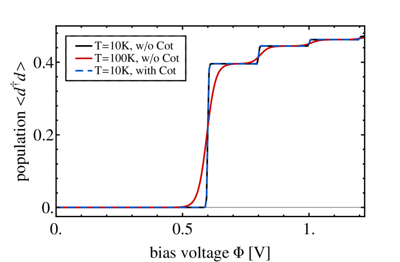
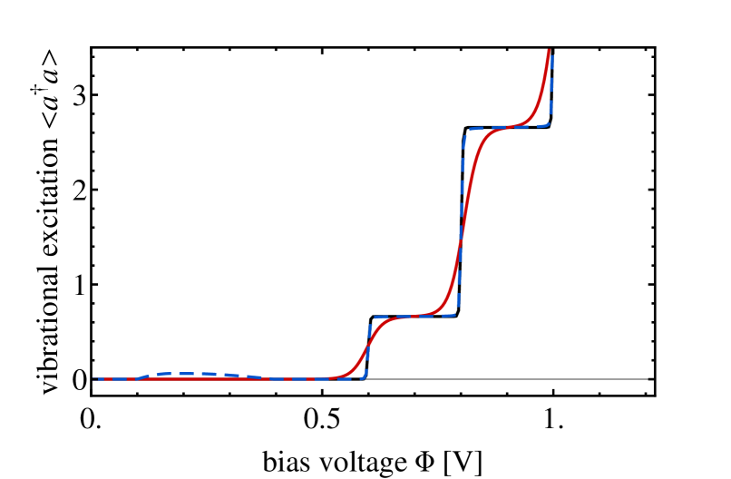
Figure 2: Electronic population and vibrational excitation characteristics of our model molecular junction (all parameters are given in the text).

For bias voltages $e\Phi<2\overline{\epsilon}_{0}$, the polaron-shifted electronic level is far above the chemical potentials in the electrodes and, therefore, exhibits no significant population. At $e\Phi\approx 2\overline{\epsilon}_{0}$, it becomes populated because the chemical potential in the left lead is high enough to allow for resonant tunneling events (which are graphically depicted Figs. 3a–c). Its population increases even further at $e\Phi\approx 2(\overline{\epsilon}_{0}+m\Omega)$ with $m\in\mathbb{N}$ due to the onset of inelastic tunneling processes, which involve the excitation of the vibrational degree of freedom by $m$ vibrational quanta during the tunneling process from the left electrode onto the molecule (see Fig. 3d for a process with a single vibrational quantum). In general, the population of the electronic level is given by the ratio of the time scales to populate and depopulate it. For $\Gamma_{\text{L}}=\Gamma_{\text{R}}$, these time scales are determined by the number and probability of tunneling processes with respect to the left and the right lead, respectively. For $e\Phi>2\overline{\epsilon}_{0}$, this ratio increases whenever a tunneling process from the left lead onto the electronic level becomes available at $e\Phi\approx 2(\overline{\epsilon}_{0}+m\Omega)$. As the probability associated with these processes decreases, the heights of the corresponding steps in the population characteristics become smaller.

(a)	(b)	(c)	(d)

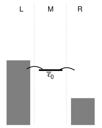
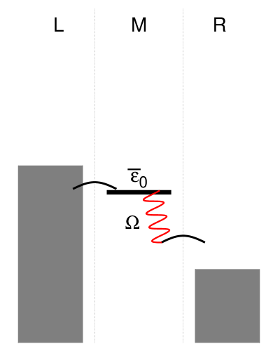
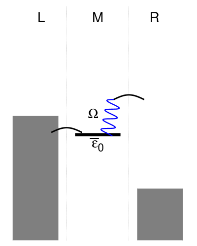
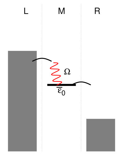
Figure 3: Graphical representation of example processes for sequential tunneling. Panel (a) depicts a sequential tunneling process where an electron from the left lead tunnels to the right lead in two resonant tunneling processes. In panel (b)/(c) the latter of the processes is accompanied by an excitation/deexcitation process where the vibrational mode is excited/deexcited by a quantum of vibrational energy. The processes (a)–(c) become active at the same bias voltage, that is for $e\Phi\approx 2\overline{\epsilon}_{0}$. The resonant excitation process shown in Panel (d) requires a higher bias voltage, that is $e\Phi\gtrsim 2(\overline{\epsilon}_{0}+\Omega)$.

Similar to the electronic population, the level of vibrational excitation increases at the same bias voltages. This quantity, however, is determined by the ratio between vibrational excitation and deexcitation processes. This includes both transport (cf. Fig. 3a–d) and electron-hole pair creation processes (cf. Fig. 4a–b). While the former are sufficient to understand the electronic population on a qualitative level, the vibrational excitation characteristics can only be understood if the effect of electron-hole pair creation processes is taken into account Härtle and Thoss (2011a, b); Härtle et al. (2013).

(a)	(b)	(c)

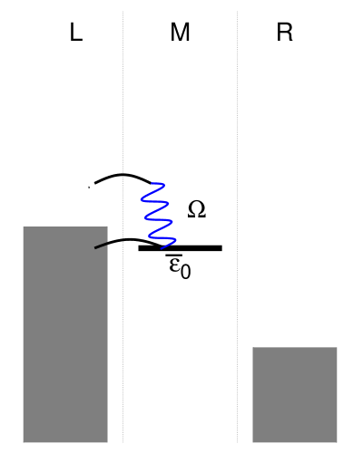
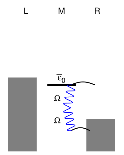
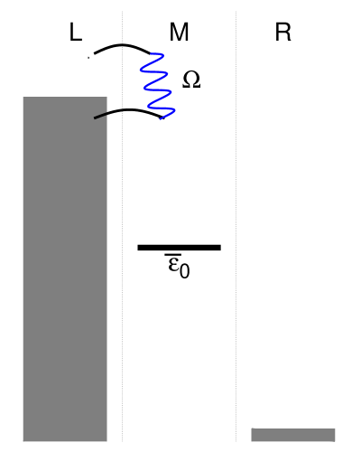
Figure 4: Graphical representation of example electron-hole pair creation processes. Panel (a) shows a resonant pair creation process, where an electron tunnels from the left lead onto the molecular bridge and back to the left lead in two sequential tunneling events, absorbing a quantum of vibrational energy. Panel (b) represents a resonant pair creation process with respect to the right lead, involving two vibrational quanta, which, for weak electronic-vibrational coupling, is less favorable than processes with only one vibrational quantum. Panel (c) depicts an off-resonant pair creation processes. These processes represent the pair creation analog of deexcitation via inelastic co-tunneling (cf. Fig. 6c).

In contrast to the electronic population, the level of vibrational excitation increases indefinitely as $\Phi\rightarrow\infty$ Härtle and Thoss (2011b). In this limit, electron-hole pair creation processes are completely suppressed and only transport processes are available. Thereby, each transport-induced excitation process is partnered by a corresponding deexcitation process (the partner of the process shown in Fig. 3b is the one depicted by Fig. 3c). Thus, the ratio between excitation and deexcitation processes is equal. This triggers a random walk through the ladder of the vibrational states Koch et al. (2006a) such that all vibrationally excited states become equally populated. As a result, the level of vibrational excitation increases indefinitely Koch et al. (2006a); Härtle and Thoss (2011b).

At finite bias voltages, electron-hole pair creation processes are active. However, they become successively suppressed if $e\Phi$ exceeds the values $2(\overline{\epsilon}_{0}+m\Omega)$ where $m\in\mathbb{Z}$ (e.g., the process shown in Fig. 4a is suppressed for $e\Phi>2(\overline{\epsilon}_{0}+\Omega)$). For small coupling strengths $\lambda$, these processes are more important the less vibrational quanta $m$ they involve. Accordingly, deexcitation of the vibrational mode via pair creation processes is most pronounced in the range of bias voltages from $e\Phi=2(\overline{\epsilon}_{0}-\Omega)$ to $e\Phi=2(\overline{\epsilon}_{0}+\Omega)$. Outside this voltage range, resonant pair creation processes require at least two vibrational quanta. At lower bias voltages, $e\Phi<2\overline{\epsilon}_{0}$, resonant deexcitation processes are more favorable than resonant excitation processes. Thus, only at higher bias voltages, $e\Phi>2(\overline{\epsilon}_{0}+\Omega)$, a significant level of vibrational excitation can develop. Thereby, for increasing bias voltages, the ratio between excitation and deexcitation processes becomes equal due to the successive suppression of pair creation processes. As a result, the step heights in the vibrational excitation characteristics do not tend to zero such as, for example, the steps in the corresponding population characteristic of the electronic level but increase with the applied bias voltage Härtle and Thoss (2011a, b).

As the pair creation processes that become suppressed at $e\Phi\approx 2(\overline{\epsilon}_{0}+m\Omega)$ with $m\in\mathbb{N}$ are more important for smaller coupling strengths $\lambda$, the level of vibrational excitation is higher when the coupling between the electronic state and the vibrational degree of freedom is weaker. This counterintuitive phenomenon has been reported by a number of groups Mitra et al. (2004); Koch et al. (2006a); Avriller (2011); Härtle and Thoss (2011b); Kast et al. (2011). It is demonstrated in Fig. 5 by the solid black line, which shows the level of vibrational excitation of our model molecular junction as a function of the electronic-vibrational coupling strength at a fixed bias voltage $e\Phi=2(\overline{\epsilon}_{0}+3\Omega/2)=0.9$ V. It can be seen that the level of vibrational excitation increases as $\lambda\rightarrow 0$. This is the situation discussed in Ref. Härtle and Thoss (2011b). There, the infinite bias limit was shown to be equal to the limit of a vanishing electronic-vibrational coupling in the sense that deexcitation due to electron-hole pair creation processes becomes suppressed. This finding does not include the effect of broadening. In the following sections, we extend these considerations to account for thermal broadening and the hybridization with the electrodes (Sec. III.2), the effect of higher-order processes (Sec. III.3) and the coupling of the vibrational mode to a thermal heat bath (Sec. III.4).

Figure 5: Level of vibrational excitation at $e\Phi=2(\overline{\epsilon}_{0}+3\Omega/2)$ as a function of the electronic-vibrational coupling strength $\lambda$. We have obtained very similar results throughout the range of bias voltages $2(\overline{\epsilon}_{0}+\Omega+k_{\text{B}}T)<e\Phi<2(\overline{\epsilon}_{0}+2\Omega-k_{\text{B}}T)$ (data not shown).

III.2 Broadening due to temperature and hybridization with the electrodes

The effect of thermal broadening can be demonstrated by recalculating the transport characteristics of our model molecular junction with an increased temperature: $T=100$ K. The corresponding electronic population and vibrational excitation characteristics are depicted by the solid red lines in Fig. 2. As compared to the black lines, the steps are much broader. Otherwise, no qualitative changes appear. This is different considering the limit $\lambda\rightarrow 0$. The red line in Fig. 5 shows a clear tendency towards a finite level of vibrational excitation for vanishing electronic-vibrational coupling (for $T=10$ K, this level is just much higher). The physical origin of this behavior can be explained in terms of electron-hole pair creation processes. Due to thermal broadening or thermal fluctuations, the suppression of electron-hole pair creation processes at $e\Phi>2(\overline{\epsilon}_{0}+m\Omega)$ is not complete. The corresponding deexcitation mechanism is not very efficient, but sufficient to keep the vibrational excitation of the junction at a finite level.

This behavior can be analyzed more rigorously using analytic arguments. To this end, we employ the Born-Markov master equation (II.2). In the limit $\lambda\rightarrow 0$ and bias voltages $e\Phi\gtrsim 2(\overline{\epsilon}_{0}+3\Omega/2)$, the resulting rate equations (II.2) can be simplified to

$$0 = \Gamma_{R}\sigma^{\nu}_{1}-\Gamma_{\text{L}}\sigma^{\nu}_{0}+\Gamma_{R}\lambda^{2}\left((\nu+1)\sigma^{\nu+1}_{1}-(2\nu+1)\sigma^{\nu}_{1}+\nu\sigma^{\nu-1}_{1}\right)$$ (25)

$$+(1-f_{\text{L}}(\epsilon_{0}+\Omega))\Gamma_{\text{L}}\lambda^{2}(\nu+1)\sigma^{\nu}_{0}$$

$$+(1-f_{\text{L}}(\epsilon_{0}+\Omega))\Gamma_{\text{L}}\lambda^{2}(\nu+1)\sigma^{\nu+1}_{1}$$

and

$$0 = \Gamma_{\text{L}}\sigma^{\nu}_{0}-\Gamma_{R}\sigma^{\nu}_{1}+\Gamma_{\text{L}}\lambda^{2}\left((\nu+1)\sigma^{\nu+1}_{0}-(2\nu+1)\sigma^{\nu}_{0}+\nu\sigma^{\nu-1}_{0}\right)$$ (26)

$$-(1-f_{\text{L}}(\epsilon_{0}+\Omega))\Gamma_{\text{L}}\lambda^{2}\nu\sigma^{\nu}_{1}$$

$$-(1-f_{\text{L}}(\epsilon_{0}+\Omega))\Gamma_{\text{L}}\lambda^{2}\nu\sigma^{\nu-1}_{0}$$

where we used the approximations $X_{\nu\nu}\approx 1-\lambda^{2}(2\nu+1)/2$, $X_{\nu\nu+1}\approx\lambda\sqrt{\nu+1}$ and evaluated each Fermi function by either $0$ or $1$ except for $f_{\text{L}}(\epsilon_{0}+\Omega)$, which allows us to take into account the most pronounced effect of thermal broadening. The corresponding term describes deexcitation via the electron-hole pair creation process depicted in Fig. 4a. For $T=0$, the equations (25) and (26) are the same as Eqs. (22) and (23) in Ref. Härtle and Thoss, 2011b. Note that contributions from the $\lambda$-dependence of $\overline{\epsilon}_{0}$ can be neglected, because the corresponding terms are of higher order or because the derivatives of the corresponding Fermi functions are evaluated at energies far from the chemical potentials.

From equations (25) and (26), we can infer that $\Gamma_{\text{R}}\sigma_{1}^{\nu}-\Gamma_{\text{L}}\sigma_{0}^{\nu}=\mathcal{O}(\lambda^{2})$. This allows us to further simplify the above equations by replacing $\Gamma_{\text{L}}\sigma_{0}^{\nu}$ with $\Gamma_{\text{R}}\sigma_{1}^{\nu}$ (if these terms are accompanied by a factor $\lambda^{2}$). The sum of the resulting equations can be written as

$$0 = +2\Gamma_{\text{R}}\left((\nu+1)\sigma^{\nu+1}_{1}-(2\nu+1)\sigma^{\nu}_{1}+\nu\sigma^{\nu-1}_{1}\right)$$

$$+(1-f_{\text{L}}(\epsilon_{0}+\Omega))\left(\Gamma_{\text{R}}(\nu+1)\sigma^{\nu}_{1}+\Gamma_{\text{L}}(\nu+1)\sigma^{\nu+1}_{1}-\Gamma_{\text{L}}\nu\sigma^{\nu}_{1}-\Gamma_{\text{R}}\nu\sigma^{\nu-1}_{1}\right).$$

The solution of this recurrence relation can be obtained with the ansatz $\sigma_{1}^{\nu+1}=\alpha\sigma_{1}^{\nu}$. It is given by

$$\sigma_{1}^{\nu+1} = \frac{1+f_{\text{L}}(\epsilon_{0}+\Omega)}{2+\frac{\Gamma_{\text{L}}}{\Gamma_{\text{R}}}(1-f_{\text{L}}(\epsilon_{0}+\Omega))}\sigma_{1}^{\nu}.$$ (28)

Similarly, one can obtain

$$\sigma_{0}^{\nu+1} = \frac{1+f_{\text{L}}(\epsilon_{0}+\Omega)}{2+\frac{\Gamma_{\text{R}}}{\Gamma_{\text{L}}}(1-f_{\text{L}}(\epsilon_{0}+\Omega))}\sigma_{0}^{\nu}.$$ (29)

For $\Gamma_{\text{R}}=\Gamma_{\text{L}}$, the corresponding level of vibrational excitation is given by

$$\langle a^{\dagger}a\rangle = (1-f_{\text{L}}(\epsilon_{0}+\Omega))^{-1}-\frac{1}{2},$$ (30)

which agrees very well with the numerical values that are shown in Fig. 5 in the limit $\lambda\rightarrow 0$.

This analysis demonstrates the importance of deexcitation via electron-hole pair creation processes. It represents an extension of the discussion given in Ref. Härtle and Thoss (2011b), where thermal broadening was not taken into account. In that case, it was shown that the limit $\lambda\rightarrow 0$ is equivalent to the high bias limit $\Phi\rightarrow\infty$, that is the level of vibrational excitation increases indefinitely in the limit $\lambda\rightarrow 0$. Including thermal broadening, however, the level of vibrational excitation does not increase indefinitely but tends to a finite value, which is determined by the probability that resonant pair creation processes can occur. This finding is similar to the one discussed in Ref. Härtle and Thoss (2011b) for lower voltages, $2(\epsilon_{0}+\Omega)>e\Phi>2(\epsilon_{0})$.

So far, we have discussed thermal broadening. The electronic level exhibits, in addition, broadening due to the coupling to the electrodes. The corresponding width is given by the sum $\Gamma_{\text{L}}+\Gamma_{\text{R}}$. This type of broadening facilitates the same deexcitation mechanisms by resonant electron-hole pair creation processes as thermal broadening and can be expected to have the same influence on the level of vibrational excitation in the weak coupling limit. We therefore conclude that the level of vibrational excitation stays finite in the limit $\lambda\rightarrow 0$. We would like emphasize that it is, nevertheless, non-zero. The latter statement is important, as it demonstrates that the level of vibrational excitation can be non-analytic in nonequilibrium situations.

III.3 Broadening due to cotunneling

As we have seen, broadening facilitates resonant electron-hole pair creation processes and that these processes are particularly important for deexcitation of the vibrational mode in the limit $\lambda\rightarrow 0$. We now investigate the role of off-resonant pair creation processes (an example is depicted in Fig. 4c) and inelastic co-tunneling processes (see Fig. 6), neglecting, at the same time, broadening effects. Recently, a direct comparison of Born-Markov and nonequilibrium Green’s function results Volkovich et al. (2011) pointed to a deexcitation mechanism via off-resonant pair creation processes which is important whenever resonant processes become suppressed. This is the case, for example, at high bias voltages where these processes result in a reduced level of vibrational excitation. Therefore, it is interesting to check the importance of these processes in the limit $\lambda\rightarrow 0$.

(a)	(b)	(c)

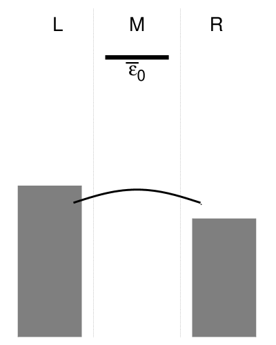
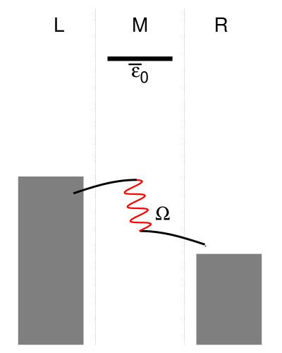
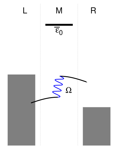
Figure 6: Graphical representation of co-tunneling processes. Panel (a) shows direct tunneling of an electron from the left to the right lead. Panel (b) and (c) depict inelastic co-tunneling, where the vibrational degree of freedom is excited and deexcited by a single quantum of vibrational energy, respectively.

We demonstrate the effect of inelastic co-tunneling and off-resonant pair creation processes by the dashed blue lines in Fig. 2. It shows the electronic population and the vibrational excitation characteristics of the model molecular junction that we already discussed in Sec. III.1. In contrast to the solid black lines, which has been obtained by the second-order rate equations (II.2), the effect of inelastic cotunneling and off-resonant pair creation processes is included in this result by employing the co-tunneling rates (II.3) and (II.3). Significant differences between the two results appear only in the non-resonant transport regime, $e\Phi<2\overline{\epsilon}_{0}$. Due to the onset of inelastic co-tunneling processes (like the one depicted by Fig. 6b), the level of vibrational excitation increases at $e\Phi=\Omega$. It decreases again at higher bias voltages, when resonant deexcitation processes require less vibrational quanta. In the resonant transport regime, the influence of these processes appears to be negligible. The latter statement is corroborated by the dashed lines in Fig. 5 (which shows the level of vibrational excitation as a function of the electronic-vibrational coupling strength in the resonant transport regime, i.e. $e\Phi=2(\overline{\epsilon}_{0}+3\Omega/2)$). They agree very well with the solid lines, which have been obtained by solving the second-order rate equations (II.2).

An analysis of the corresponding rate equations allows us to elucidate this point more clearly. In the limit $\lambda\rightarrow 0$ and bias voltages $e\Phi\gtrsim 2(\overline{\epsilon}_{0}+3\Omega/2)$, the rate equations (II.3) can be simplified to

$$0 = \Gamma_{\text{R}}\sigma^{\nu}_{1}-\Gamma_{\text{L}}\sigma^{\nu}_{0}+\Gamma_{\text{R}}\lambda^{2}\left((\nu+1)\sigma^{\nu+1}_{1}-(2\nu+1)\sigma^{\nu}_{1}+\nu\sigma^{\nu-1}_{1}\right)$$

$$-\lambda^{2}\left((\nu+1)W_{\nu\rightarrow\nu+1}+\nu W_{\nu\rightarrow\nu-1}\right)\sigma^{\nu}_{0}$$

$$+\lambda^{2}\left((\nu+1)W_{\nu\rightarrow\nu+1}\sigma^{\nu+1}_{0}+\nu W_{\nu\rightarrow\nu-1}\sigma^{\nu-1}_{0}\right)$$

and

$$0 = \Gamma_{\text{L}}\sigma^{\nu}_{0}-\Gamma_{\text{R}}\sigma^{\nu}_{1}+\Gamma_{\text{L}}\lambda^{2}\left((\nu+1)\sigma^{\nu+1}_{0}-(2\nu+1)\sigma^{\nu}_{0}+\nu\sigma^{\nu-1}_{0}\right)$$

$$-\lambda^{2}\left((\nu+1)W_{\nu\rightarrow\nu-1}+\nu W_{\nu\rightarrow\nu+1}\right)\sigma^{\nu}_{1}$$

$$+\lambda^{2}\left((\nu+1)W_{\nu\rightarrow\nu-1}\sigma^{\nu+1}_{1}+\nu W_{\nu\rightarrow\nu+1}\sigma^{\nu-1}_{1}\right),$$

where we used $W_{\nu\rightarrow\nu\pm 1}=\sum_{K,K^{\prime}}\gamma_{K\rightarrow K^{\prime},0\rightarrow 0}^{\nu\rightarrow\nu\pm 1}=\sum_{K,K^{\prime}}\gamma_{K\rightarrow K^{\prime},1\rightarrow 1}^{\nu\rightarrow\nu\mp 1}$ and, in contrast to our analysis in Sec. III.2, we neglect thermal broadening, that is we evaluate each Fermi funtion by either 0 or 1 (including $f_{\text{L}}(\overline{\epsilon}_{0}+\Omega)$). Arguing again that $\Gamma_{\text{R}}\sigma_{1}^{\nu}-\Gamma_{\text{L}}\sigma_{0}^{\nu}=\mathcal{O}(\lambda^{2})$, we can further simplify these equations and obtain

$$0 = \left(2\Gamma_{\text{R}}+\frac{\Gamma_{\text{R}}}{\Gamma_{\text{L}}}W_{\nu\rightarrow\nu+1}+W_{\nu\rightarrow\nu-1}\right)(\nu+1)\sigma_{1}^{\nu+1}+\left(2\Gamma_{\text{R}}+\frac{\Gamma_{\text{R}}}{\Gamma_{\text{L}}}W_{\nu\rightarrow\nu-1}+W_{\nu\rightarrow\nu+1}\right)\nu\sigma^{\nu-1}_{1}$$

$$-\left(2\Gamma_{\text{R}}(2\nu+1)+\frac{\Gamma_{\text{R}}}{\Gamma_{\text{L}}}\left((\nu+1)W_{\nu\rightarrow\nu+1}+\nu W_{\nu\rightarrow\nu-1}\right)+\left((\nu+1)W_{\nu\rightarrow\nu-1}+\nu W_{\nu\rightarrow\nu+1}\right)\right)\sigma^{\nu}_{1}.$$

The solution of this recurrence relation is

$$\sigma_{1/0}^{\nu+1}=\sigma_{1/0}^{\nu}.$$ (34)

which corresponds to an equal population of the vibrational levels and, therefore, to an infinite level of vibrational excitation. This result shows that, in the range of bias voltages considered, the ratio between excitation and deexcitation processes due to off-resonant pair creation and inelastic cotunneling processes is the same if broadening effects are explicitly excluded. Thus, the system exhibits a random walk through the ladder of all vibrational states, leading to the vibrational instability that has already been outlined in Refs. Koch et al. (2006a); Härtle and Thoss (2011b). We think this is an important finding, because broadening is typically understood in terms of these processes. An implementation of these processes in terms of the rates (II.3) and (II.3) is often very useful. Our results show that this procedure has to be applied with care, as it can lead to qualitatively incorrect results for the level of vibrational excitation in the weak coupling limit $\lambda\rightarrow 0$.

III.4 Broadening due to coupling to a heat bath

In the previous sections, we were disregarding the effect of dissipation due to the coupling of the vibrational mode to a secondary bath of phonon modes (heat bath). We now include these effects via a non-zero dissipation rate $\gamma_{\text{bath}}$, solving the rate equations (II.2). Fig. 7 depicts the corresponding level of vibrational excitation of our model molecular junction as a function of the electronic-vibrational coupling strength for different values of the dissipation rate $\gamma_{\text{bath}}$.

The coupling to a heat bath appears to be particularly important for weak electronic-vibrational coupling strengths. In particular for $\lambda\rightarrow 0$, it leads to an analytic behavior of this observable. The corresponding level of vibrational excitation tends towards the equilibrium value $(\text{exp}(\Omega/(k_{\text{B}}T))-1)^{-1}$. This behavior is independent of the value of $\gamma_{\text{bath}}$. The non-analytic behavior that we described before can therefore be considered to be an artifact of the model, where the dissipative effect of the environment on the local vibrational mode is neglected. Physical systems will always exhibit such coupling and, consequently, an analytic behavior of the level of vibrational excitation in the limit of vanishing electronic-vibrational coupling.

Our results also show that a negative slope of the level of vibrational excitation is obtained as long as the value of the dissipation rate $\gamma_{\text{bath}}$ is smaller than the excitation rate $\lambda^{2}\Gamma/\Omega^{2}$. A negative slope is not observed, once the coupling to the heat bath quenches the level of vibrational excitation also for strong electronic-vibrational coupling strengths $\lambda/\Omega\sim 1$.

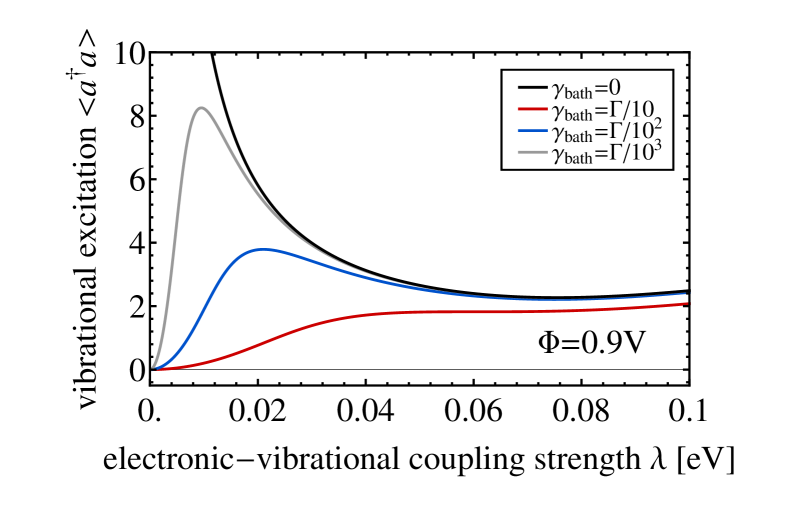
Figure 7: Level of vibrational excitation at $e\Phi=2(\overline{\epsilon}_{0}+3\Omega/2)$ as a function of the electronic-vibrational coupling strength $\lambda$ for different dissipation rates $\gamma_{\text{bath}}$.

IV Conclusions

We have studied the level of vibrational excitation in a model molecular junction with a single electronic state that is coupled to a single vibrational mode. We find that the level of vibrational excitation increases for a decreasing electronic-vibrational coupling strength, if deexcitation of the vibrational mode (local cooling) via electron-hole pair creation processes is suppressed by high enough bias voltages and if the coupling of the vibrational mode to a bath of secondary modes is not too strong. In the limit of vanishing electronic-vibrational coupling and without dissipation, the level of vibrational excitation is non-zero and exhibits non-analytic behavior. The corresponding value is finite and determined by the probability that electron-hole pair creation processes can occur. The latter is strongly influenced by the broadening of the junction’s energy levels either due to thermal broadening or the hybridization with the Fermi sea of the electrodes. Including the coupling to a heat bath, the non-analytic behavior does not occur irrespective of the associated coupling strength, that is the non-analytic behavior is an artifact of neglecting the influence of the environment on the local vibrational mode.

Our findings are based on numerical and analytical results derived from Born-Markov theory. In addition, we considered transition rates corresponding to higher-order processes corresponding to, for example, off-resonant pair creation or inelastic cotunneling. While these processes can account for excitation and deexcitation mechanisms in the non-resonant transport regime, we have shown that a more rigorous treatment is necessary in the resonant regime. There, a treatment of these processes in terms of virtual tunneling processes, where broadening effects are explicitly excluded, leads to the same result as the one that is obtained from Born-Markov theory.

At this point, we emphasize that a similar behavior of the level of vibrational excitation is found in the presence of a second higher-lying electronic state Härtle and Thoss (2011b). This is of particular interest in the present context, as the photon number in cQED systems has been measured in double quantum dot setups, using the spin-torque effect Viennot et al. (2014). Future directions of research should therefore include the description of the level of vibrational excitation / photon number in the weak coupling limit of these more complex systems, including the effect of electron-electron interactions. Moreover, it may be interesting to develop schemes that allow to extract the photon number in single dot systems.

References

- Schäfer and Wegener (2002) M. Schäfer and M. Wegener, Semiconductor Optics and Transport Phenomena (Springer, Berlin Heidelberg New York, 2002).
- Delbecq et al. (2011) M. R. Delbecq, V. Schmitt, F. D. Parmentier, N. Roch, J. J. Viennot, G. Fève, B. Huard, C. Mora, A. Cottet, and T. Kontos, Phys. Rev. Lett. 107, 256804 (2011).
- Mahan (1981) G. D. Mahan, Many-Particle Physics (Plenum Press, New York, 1981).
- Raimond et al. (2001) J. M. Raimond, M. Brune, and S. Haroche, Rev. Mod. Phys. 73, 565 (2001).
- Wallraff et al. (2004) A. Wallraff, D. I. Schuster, A. Blais, L. Frunzio, R. Huang, J. Majer, S. Kumar, S. M. Girvin, and R. J. Schoelkopf, Nature 431, 162 (2004).
- Chiorescu et al. (2004) I. Chiorescu, P. Bertet, K. Semba, Y. Nakamura, C. J. P. M. Harmans, and J. E. Mooij, Nature 431, 159 (2004).
- Koch et al. (2006a) J. Koch, M. Semmelhack, F. von Oppen, and A. Nitzan, Phys. Rev. B 73, 155306 (2006a).
- Härtle et al. (2009) R. Härtle, C. Benesch, and M. Thoss, Phys. Rev. Lett. 102, 146801 (2009).
- Härtle and Thoss (2011a) R. Härtle and M. Thoss, Phys. Rev. B 83, 115414 (2011a).
- Romano et al. (2010) G. Romano, A. Gagliardi, A. Pecchia, and A. Di Carlo, Phys. Rev. B 81, 115438 (2010).
- Schiró and Le Hur (2014) M. Schiró and K. Le Hur, Phys. Rev. B 89, 195127 (2014).
- Abdullah et al. (2014) N. R. Abdullah, C. Tang, A. Manolescu, and V. Gudmundsson, Physica E 64, 254 (2014).
- Kulkarni et al. (2014) M. Kulkarni, O. Cotlet, and H. E. Türeci, Phys. Rev. B 90, 125402 (2014).
- Schinabeck et al. (2014) C. Schinabeck, R. Härtle, H. B. Weber, and M. Thoss, Phys. Rev. B 90, 075409 (2014).
- Boese and Schoeller (2001) D. Boese and H. Schoeller, Europhys. Lett. 54, 668 (2001).
- Cuniberti et al. (2005) G. Cuniberti, G. Fagas, and K. Richter, Introducing Molecular Electronics (Springer, Heidelberg, 2005).
- Koch and von Oppen (2005) J. Koch and F. von Oppen, Phys. Rev. B 72, 113308 (2005).
- Zazunov et al. (2006) A. Zazunov, D. Feinberg, and T. Martin, Phys. Rev. B 73, 115405 (2006).
- Galperin et al. (2009) M. Galperin, K. Saito, A. V. Balatsky, and A. Nitzan, Phys. Rev. B 80, 115427 (2009).
- Leijnse and Wegewijs (2008) M. Leijnse and M. R. Wegewijs, Phys. Rev. B 78, 235424 (2008).
- Cuevas and Scheer (2010) J. C. Cuevas and E. Scheer, Molecular Electronics: An Introduction To Theory And Experiment (World Scientific, Singapore, 2010).
- Wang et al. (2012) C. Wang, J. Ren, W. Li, and Q. H. Chen, Eur. Phys. J. B 85, 110 (2012).
- Härtle et al. (2013) R. Härtle, U. Peskin, and M. Thoss, Phys. Status Solidi B 250, 2365 (2013).
- Skolnick and Mowbray (2004) M. S. Skolnick and D. J. Mowbray, Ann. Rev. Mater. Res. 34, 181 (2004).
- Schoelkopf and Girvin (2008) R. J. Schoelkopf and M. S. Girvin, Nature 451, 664 (2008).
- Juska et al. (2013) G. Juska, V. Dimastrodonato, L. O. Mereni, A. Gocalinska, and E. Pelucchi, Nature Photonics 7, 527 (2013).
- Selinsky et al. (2013) R. S. Selinsky, Q. Ding, M. S. Faber, J. C. Wright, and S. Jin, Chem. Soc. Rev. 42, 2963 (2013).
- Wang et al. (2014) C. Wang, J. Ren, and J. Cao, New J. Phys. 16, 045019 (2014).
- Wu and Wang (2014) J. Wu and Z. M. Wang, Quantum Dot Solar Cells (Springer, New York, 2014).
- Ajisaka et al. (2015) S. Ajisaka, B. Zunkovic, and Y. Dubi, Sci. Rep. 5, 5 (2015).
- Brumer and Shapiro (2003) P. W. Brumer and M. Shapiro, Principles of the Quantum Control of Molecular Processes (Wiley, New Jersey, 2003).
- Pascual et al. (2003) J. I. Pascual, N. Lorente, Z. Song, H. Conrad, and H. P. Rust, Nature 423, 525 (2003).
- Härtle et al. (2010) R. Härtle, R. Volkovich, M. Thoss, and U. Peskin, J. Chem. Phys. 133, 081102 (2010).
- Dzhioev and Kosov (2011) A. A. Dzhioev and D. S. Kosov, J. Chem. Phys. 135, 074701 (2011).
- Volkovich et al. (2011) R. Volkovich, R. Härtle, M. Thoss, and U. Peskin, Phys. Chem. Chem. Phys. 13, 14333 (2011).
- Nitzan (2001) A. Nitzan, Annu. Rev. Phys. Chem. 52, 681 (2001).
- Tao (2006) N. J. Tao, Nat. Nano. 1, 173 (2006).
- Selzer and Allara (2006) Y. Selzer and D. L. Allara, Annu. Rev. Phys. Chem. 57, 593 (2006).
- Chen et al. (2007) F. Chen, J. Hihath, Z. Huang, X. Li, and N. J. Tao, Annu. Rev. Phys. Chem. 58, 535 (2007).
- May (2002) V. May, Phys. Rev. B 66, 245411 (2002).
- Flensberg (2003) K. Flensberg, Phys. Rev. B 68, 205323 (2003).
- Mitra et al. (2004) A. Mitra, I. Aleiner, and A. J. Millis, Phys. Rev. B 69, 245302 (2004).
- Wu et al. (2004) S. W. Wu, G. V. Nazin, X. Chen, X. H. Qiu, and W. Ho, Phys. Rev. Lett. 93, 236802 (2004).
- Galperin et al. (2004) M. Galperin, M. A. Ratner, and A. Nitzan, J. Chem. Phys. 121, 11965 (2004).
- Frederiksen et al. (2004) T. Frederiksen, M. Brandbyge, N. Lorente, and A. P. Jauho, Phys. Rev. Lett. 93, 256601 (2004).
- Cizek et al. (2004) M. Cizek, M. Thoss, and W. Domcke, Phys. Rev. B 70, 125406 (2004).
- Wegewijs and Nowack (2005) M. R. Wegewijs and K. C. Nowack, New J. Phys. 7, 239 (2005).
- Galperin et al. (2007) M. Galperin, M. A. Ratner, and A. Nitzan, J. Phys.: Condens. Matter 19, 103201 (2007).
- Avriller and Levy Yeyati (2009) R. Avriller and A. Levy Yeyati, Phys. Rev. B 80, 041309 (2009).
- Schmidt and Komnik (2009) T. L. Schmidt and A. Komnik, Phys. Rev. B 80, 041307 (2009).
- Haupt et al. (2009) F. Haupt, T. Novotný, and W. Belzig, Phys. Rev. Lett. 103, 136601 (2009).
- Koch et al. (2010) T. Koch, J. Loos, A. Alvermann, A. R. Bishop, and H. Fehske, Journal of Physics: Conference Series 220, 012014 (2010).
- Urban et al. (2010) D. F. Urban, R. Avriller, and A. Levy Yeyati, Phys. Rev. B 82, 121414 (2010).
- Entin-Wohlman et al. (2010) O. Entin-Wohlman, Y. Imry, and A. Aharony, Phys. Rev. B 81, 113408 (2010).
- Esposito and Galperin (2010) M. Esposito and M. Galperin, J. Phys. Chem. C 114, 20362 (2010).
- Dash et al. (2012) L. K. Dash, H. Ness, M. J. Verstraete, and R. W. Godby, J. Chem. Phys. 136, 064708 (2012).
- Yu et al. (2004) L. H. Yu, Z. K. Keane, J. W. Ciszek, L. Cheng, M. P. Stewart, J. M. Tour, and D. Natelson, Phys. Rev. Lett. 93, 266802 (2004).
- Kushmerick et al. (2004) J. G. Kushmerick, J. Lazorcik, C. H. Patterson, R. Shashidhar, D. S. Seferos, and G. C. Bazan, Nano Lett. 4, 639 (2004).
- Qiu et al. (2004) X. H. Qiu, G. V. Nazin, and W. Ho, Phys. Rev. Lett. 92, 206102 (2004).
- Sapmaz et al. (2005) S. Sapmaz, P. Jarillo-Herrero, Y. M. Blanter, and H. S. J. van der Zant, New J. Phys. 7, 243 (2005).
- Pasupathy et al. (2005) A. N. Pasupathy, J. Park, C. Chang, A. V. Soldatov, S. Lebedkin, R. C. Bialczak, J. E. Grose, L. A. K. Donev, J. P. Sethna, D. C. Ralph, and P. L. McEuen, Nano Lett. 5, 203 (2005).
- Sapmaz et al. (2006) S. Sapmaz, P. Jarillo-Herrero, Y. M. Blanter, C. Dekker, and H. S. J. van der Zant, Phys. Rev. Lett. 96, 026801 (2006).
- Thijssen et al. (2006) W. H. A. Thijssen, D. Djukic, A. F. Otte, R. H. Bremmer, and J. M. van Ruitenbeek, Phys. Rev. Lett. 97, 226806 (2006).
- Parks et al. (2007) J. J. Parks, A. R. Champagne, G. R. Hutchison, S. Flores-Torres, H. D. Abruna, and D. C. Ralph, Phys. Rev. Lett. 99, 026601 (2007).
- Böhler et al. (2007) T. Böhler, A. Edtbauer, and E. Scheer, Phys. Rev. B 76, 125432 (2007).
- de Leon et al. (2008) N. P. de Leon, W. Liang, Q. Gu, and H. Park, Nano Lett. 8, 2963 (2008).
- Repp et al. (2010) J. Repp, P. Liljeroth, and G. Meyer, Nature Physics 6, 975 (2010).
- Hüttel et al. (2009) A. K. Hüttel, B. Witkamp, M. Leijnse, M. R. Wegewijs, and H. S. J. van der Zant, Phys. Rev. Lett. 102, 225501 (2009).
- Hihath et al. (2010) J. Hihath, C. Bruot, and N. Tao, ACS Nano 4, 3823 (2010).
- Ballmann et al. (2010) S. Ballmann, W. Hieringer, D. Secker, Q. Zheng, J. A. Gladysz, A. Görling, and H. B. Weber, ChemPhysChem 11, 2256 (2010).
- Ward et al. (2008) D. R. Ward, N. J. Halas, J. W. Ciszek, J. M. Tour, Y. Wu, P. Nordlander, and D. Natelson, Nano Lett. 8, 919 (2008).
- Ioffe et al. (2008) Z. Ioffe, T. Shamai, A. Ophir, G. Noy, I. Yutsis, K. Kfir, O. Cheshnovsky, and Y. Selzer, Nat. Nano. 3, 727 (2008).
- Ward et al. (2011) D. R. Ward, D. A. Corley, J. M. Tour, and D. Natelson, Nature Nanotechnology 6, 33 (2011).
- Yoshie et al. (2004) T. Yoshie, A. Scherer, J. Hendrickson, G. Khitrova, H. M. Gibbs, G. Rupper, C. Ell, O. B. Shchekin, and D. G. Deppe, Nature 432, 200 (2004).
- Reithmaier et al. (2004) J. P. Reithmaier, G. Se ogonk, A. Löffler, C. Hofmann, S. Kuhn, S. Reitzenstein, L. V. Keldysh, V. D. Kulakovskii, T. L. Reinecke, and A. Forchel, Nature 432, 197 (2004).
- Petersson et al. (2011) K. D. Petersson, L. W. McFaul, M. D. Schroer, M. Jung, J. M. Taylor, A. A. Houck, and J. R. Petta, Nature 490, 380 (2011).
- Delbecq et al. (2013) M. R. Delbecq, L. E. Bruhat, J. J. Viennot, S. Datta, A. Cottet, and T. Kontos, Nat. Commun. 4, 1400 (2013).
- Liu et al. (2014) Y. Y. Liu, K. D. Petersson, J. Stehlik, J. M. Taylor, and J. R. Petta, Phys. Rev. Lett. 113, 036801 (2014).
- Viennot et al. (2014) J. J. Viennot, M. R. Delbecq, M. C. Dartiailh, A. Cottet, and T. Kontos, Phys. Rev. B 89, 165404 (2014).
- Cottet et al. (2015) A. Cottet, T. Kontos, and P. Doucot, , arXiv:1501.00803 (2015).
- Avriller (2011) R. Avriller, J. Phys.: Condens. Matter 23, 105301 (2011).
- Härtle and Thoss (2011b) R. Härtle and M. Thoss, Phys. Rev. B 83, 125419 (2011b).
- Kast et al. (2011) D. Kast, L. Kecke, and J. Ankerhold, Beilstein J. Nanotechnol. 2, 416 (2011).
- Koch et al. (2006b) J. Koch, F. von Oppen, and A. V. Andreev, Phys. Rev. B 74, 205438 (2006b).
- Lüffe et al. (2008) M. C. Lüffe, J. Koch, and F. von Oppen, Phys. Rev. B 77, 125306 (2008).
- Weiss (1993) U. Weiss, Quantum Dissipative Systems (World Scientific, Singapore, 1993).
- Thoss and Domcke (1998) M. Thoss and W. Domcke, J. Chem. Phys. 109, 6577 (1998).
- Härtle et al. (2008) R. Härtle, C. Benesch, and M. Thoss, Phys. Rev. B 77, 205314 (2008).
- Jorn and Seidemann (2009) R. Jorn and T. Seidemann, J. Chem. Phys. 131, 244114 (2009).
- Mukamel and Smalley (1980) S. Mukamel and R. E. Smalley, J. Chem. Phys. 73, 4156 (1980).
- Freed and Nitzan (1983) K. F. Freed and A. Nitzan, Energy Storage and Redistribution in Molecules (Plenum, New York, 1983).
- Zewail (1994) A. H. Zewail, Femtochemistry – Ultrafast Dynamics of the Chemical Bond (World Scientific, Singapore, 1994).
- Nesbitt and Field (1996) D. J. Nesbitt and R. W. Field, J. Phys. Chem. 100, 12735 (1996).
- Galperin et al. (2006) M. Galperin, A. Nitzan, and M. A. Ratner, Phys. Rev. B 73, 045314 (2006).
- Lehmann et al. (2004) J. Lehmann, S. Kohler, V. May, and P. Hänggi, J. Chem. Phys. 121, 2278 (2004).
- Harbola et al. (2006) U. Harbola, M. Esposito, and S. Mukamel, Phys. Rev. B 74, 235309 (2006).
- Volkovich et al. (2008) R. Volkovich, M. Caspary Toroker, and U. Peskin, J. Chem. Phys. 129, 034501 (2008).
- Nakajima (1958) S. Nakajima, Prog. Theor. Phys. 20, 948 (1958).
- Zwanzig (1960) R. Zwanzig, J. Chem. Phys. 33, 1338 (1960).
- Härtle and Millis (2014) R. Härtle and A. J. Millis, Phys. Rev. B 90, 245426 (2014).
- Pedersen and Wacker (2005) J. N. Pedersen and A. Wacker, Phys. Rev. B 72, 195330 (2005).