Stability and symmetry breaking in a three-Higgs-doublet model with lepton family symmetry $O(2)\otimes\mathbbm{Z}_{2}$

Abstract

Motivated by the neutrino data, an extension of the Standard Model with three Higgs-boson doublets has been proposed. Imposing an $O(2)\otimes\mathbbm{Z}_{2}$ family symmetry, a neutrino mixing matrix with $\theta_{23}=\pi/4$ and $\theta_{13}=0$ appears in a natural way. Even though these values for the mixing matrix do not follow the recent experimental constraints, they are nevertheless a good approximation. We study the Higgs potential of this model in detail. We apply recent methods which allow for the study of any three-Higgs-boson doublet model. It turns out that for a variety of parameters the potential is stable, has the correct electroweak symmetry breaking, and gives the correct vacuum expectation value.

1 The $O(2)\otimes\mathbbm{Z}_{2}$ model

The experimental neutrino mixing data show that the neutrino mixing is very different from the quark mixing. In the usual parametrization of the neutrino mixing matrix (see for instance Agashe:2014kda ), experimental data suggest that the angle $\theta_{13}$ is small (but nonzero), and $\theta_{23}$ is close to $\pi/4$ GonzalezGarcia:2012sz .

There is lot of effort spent on finding an organizing principle for the flavor puzzle. A general approach is to study finite subgroups of SU(3) which have an irreducible triplet representation; see for instance King:2013eh and references therein. Examples of subgroups with triplet representations are $S_{4}$, the group of permutations of 4 elements, with two singlet, one doublet, and two triplet representations (see for instance Ma:2005pd ); or $A_{4}$, the group of even permutations of 4 elements which has also a triplet representation besides singlet representations (see for instance Ma:2009wi ; Felipe:2013vwa ); or $\Delta(27)$, with 27 elements and two triplet representations (see for instance Ma:2013xqa ).

In contrast, here we want to study in detail the Higgs potential of a three Higgs-boson-doublet model which imposes a $O(2)\times\mathbbm{Z}_{2}$ symmetry – without any irreducible triplet representation. Let us closely follow the motivation of Grimus:2008dr . The starting point is a neutrino mass matrix which is symmetric in generations two and three,

$$M_{\nu}=\begin{pmatrix}x&y&y\\ y&z&w\\ y&w&z\end{pmatrix}.$$ (1)

This mass matrix may be diagonalized as usual, that is, $U^{\dagger}M_{\nu}U=\operatorname{diag}(m_{\nu_{1}}^{2},m_{\nu_{2}}^{2},m_{\nu_{3}}^{2})$, where $U$ is the neutrino mixing matrix and $m_{\nu_{1}}$, $m_{\nu_{2}}$, $m_{\nu_{3}}$ the neutrino masses. Expressing the mixing matrix $U$ in terms of the usual parametrization Agashe:2014kda , we get in particular $\theta_{13}=0$ and $\theta_{23}=\pi/4$. Even though the experimental results are not in exact agreement with these values, in particular $\theta_{13}$ is nonzero, they at least appear to be approximately fulfilled. We note that deviations from these approximate values for the mixing angles could arise by soft-symmetry-breaking terms or beyond-leading-order effects; see for instance the study in Altarelli:2010gt .

The mass matrix (1) may be generated by the introduction of three Higgs-boson doublets $\varphi_{i}$, $i=1,2,3$, and a symmetry $O(2)\times\mathbbm{Z}_{2}\cong\mathbbm{Z}_{2}^{\prime}\times\mathbbm{Z}_{2}\times U(1)$, where all elementary particles are assigned to an appropriate transformation behavior on this symmetry. The reflection symmetry $\mathbbm{Z}_{2}^{\prime}$ is responsible for the $\mu$–$\tau$ symmetry of $\eqref{massmatrix}$:

$$\mathbbm{Z}_{2}^{\prime}:\quad D_{\mu L}\leftrightarrow D_{\tau L},\;\mu_{R}\leftrightarrow\tau_{R},\;\nu_{\mu R}\leftrightarrow\nu_{\tau R},\;\phi_{1}\leftrightarrow\phi_{2}$$ (2)

Here $$D_{\mu L} D_{\tau L} SU(2) \nu_{\mu R} \nu_{\tau R} \mathbbm{Z}_{2}^{\prime} \mathbbm{Z}_{2}$$ and denote the left-handed lepton doublets, and the right-handed neutrinos, and all remaining fields transform trivially under the symmetry. The symmetry is given by a sign change,

$$\mathbbm{Z}_{2}: \nu_{eR}\rightarrow-\nu_{eR},\;\nu_{\mu R}\rightarrow-\nu_{\mu R},\;\nu_{\tau R}\rightarrow-\nu_{\tau R},$$

$$e_{R}\rightarrow-e_{R},\;\varphi_{3}\rightarrow-\varphi_{3},$$ (3)

with $$\nu_{eR} \nu_{\mu R} \nu_{\tau R} e_{R} \mathbbm{Z}_{2} U(1)$$, , the right-handed neutrinos, the right-handed electron, and all other fields unchanged under this symmetry. Eventually the assignment with respect to the phase symmetry is

$$U(1): \begin{array}[]{c|cccc}X\longrightarrow e^{i\theta}X&D_{\mu L},\tau_{R},\nu_{\mu R}&\,D_{\tau L},\mu_{R},\nu_{\tau R}&\,\varphi_{1}&\,\varphi_{2}\\ \hline\cr\theta&1&-1&2&-2\end{array}$$ (6)

with $X$ one of the fields on the right-hand side of the table transforming as $X\longrightarrow e^{i\theta}X$ with the corresponding phase $\theta$ given explicitly in the table. All other fields transform trivially.

By virtue of these symmetries – besides the electroweak $SU(2)_{L}\times U(1)_{Y}$ symmetry – there appear in particular the invariant Yukawa couplings

$${\mathscr{L}}_{Y}=-y_{4}\left(\bar{D}_{\mu L}\varphi_{1}\mu_{R}+\bar{D}_{\tau L}\varphi_{2}\tau_{R}\right)+h.c.$$ (7)

The most general potential for the three Higgs-boson doublets $\varphi_{1}$, $\varphi_{2}$, $\varphi_{3}$ reads

$$V_{O(2)\times\mathbbm{Z}_{2}}=\mu_{0}\varphi_{3}^{\dagger}\varphi_{3}+\mu_{12}\left(\varphi_{1}^{\dagger}\varphi_{1}+\varphi_{2}^{\dagger}\varphi_{2}\right)\\ +\mu_{m}\left(\varphi_{1}^{\dagger}\varphi_{2}+\varphi_{2}^{\dagger}\varphi_{1}\right)+a_{1}(\varphi_{3}^{\dagger}\varphi_{3})^{2}\\ +a_{2}\varphi_{3}^{\dagger}\varphi_{3}\left(\varphi_{1}^{\dagger}\varphi_{1}+\varphi_{2}^{\dagger}\varphi_{2}\right)\\ +a_{3}\left(\varphi_{3}^{\dagger}\varphi_{1}\cdot\varphi_{1}^{\dagger}\varphi_{3}+\varphi_{3}^{\dagger}\varphi_{2}\cdot\varphi_{2}^{\dagger}\varphi_{3}\right)\\ +a_{4}\varphi_{3}^{\dagger}\varphi_{1}\cdot\varphi_{3}^{\dagger}\varphi_{2}+a_{4}^{*}\varphi_{1}^{\dagger}\varphi_{3}\cdot\varphi_{2}^{\dagger}\varphi_{3}\\ +a_{5}\left((\varphi_{1}^{\dagger}\varphi_{1})^{2}+(\varphi_{2}^{\dagger}\varphi_{2})^{2}\right)\\ +a_{6}\varphi_{1}^{\dagger}\varphi_{1}\cdot\varphi_{2}^{\dagger}\varphi_{2}+a_{7}\varphi_{1}^{\dagger}\varphi_{2}\cdot\varphi_{2}^{\dagger}\varphi_{1},$$ (8)

where the term $\mu_{m}(\varphi_{1}^{\dagger}\varphi_{2}+\varphi_{2}^{\dagger}\varphi_{1})$ breaks the $U(1)$ symmetry (6) explicitly but softly, since this is a quadratic term. For a nonvanishing parameter $\mu_{m}$ in this way additional Goldstone bosons are avoided, which otherwise would appear by spontaneous symmetry breaking of the $U(1)$ symmetry. This potential has nine real parameters and one complex parameter $a_{4}$, corresponding to eleven real parameters in total.

Now we want to discuss stability, stationarity, and electroweak symmetry breaking of this model. Of course only a model with a stable potential, having the correct-electroweak-symmetry-breaking behavior and the correct vacuum expectation values is physically acceptable. These obvious constraints restrict the parameter space of the potential. Here, we focus on the Higgs potential and not on any further experimental limits. For instance, the expressions for the oblique parameters $S$, $T$, $U$ are available for any nHDM Grimus:2007if and may be compared to the electroweak precision data.

Since the $O(2)\otimes\mathbbm{Z}_{2}$ model is a 3HDM we encounter in this model four charged Higgs bosons and in total five neutral Higgs bosons. We expect a changed phenomenology of this model compared to the Standard Model. Of course, the detection of any further Higgs boson would be a clear signal for a model beyond the Standard Model. Depending on the Yukawa coupling strength in (1.5) we have for instance the signature of the production of a charged Higgs boson with subsequent decay into a muon and a muon-neutrino. The potential itself is in principle detectable via its trilinear and quartic Higgs self-couplings. We leave this investigation for future work and focus here on the study of the Higgs potential with respect to stability, electroweak symmetry breaking and the global minimum.

Even though the potential (8) appears to be rather involved we will see that it is indeed accessible in the bilinear approach Nagel:2004sw ; Maniatis:2006fs ; Nishi:2006tg . In this approach gauge degrees of freedom are avoided systematically. Moreover, the corresponding equations for stability and stationarity simplify in particular, the degree of systems of equations is lowered. Recently, the bilinear approach for the study of stability, stationarity, and electroweak symmetry breaking has been extended to the study of any 3HDM Maniatis:2014oza , which we now briefly review.

The scalar products of the type $\varphi_{i}^{\dagger}\varphi_{j}$, $i,j\in\{1,2,3\}$, in the potential (8) may be arranged in a $3\!\times\!3$ matrix

$$\underline{K}=\begin{pmatrix}\varphi_{1}^{\dagger}\varphi_{1}&\varphi_{2}^{\dagger}\varphi_{1}&\varphi_{3}^{\dagger}\varphi_{1}\\ \varphi_{1}^{\dagger}\varphi_{2}&\varphi_{2}^{\dagger}\varphi_{2}&\varphi_{3}^{\dagger}\varphi_{2}\\ \varphi_{1}^{\dagger}\varphi_{3}&\varphi_{2}^{\dagger}\varphi_{3}&\varphi_{3}^{\dagger}\varphi_{3}\end{pmatrix}.$$ (9)

By the introduction of the bilinears,

$$K_{\alpha}=K_{\alpha}^{*}=\operatorname{tr}(\underline{K}\lambda_{\alpha}),\qquad\alpha=0,...,8$$ (10)

with $\lambda_{\alpha}$ the $3\!\times\!3$ Gell-Mann matrices, the following replacements can be made in the potential:

$$\varphi_{1}^{\dagger}\varphi_{1}=\frac{K_{0}}{\sqrt{6}}+\frac{K_{3}}{2}+\frac{K_{8}}{2\sqrt{3}},\qquad \varphi_{1}^{\dagger}\varphi_{2}=\frac{1}{2}\left(K_{1}+iK_{2}\right),$$

$$\varphi_{1}^{\dagger}\varphi_{3}=\frac{1}{2}\left(K_{4}+iK_{5}\right),\qquad \varphi_{2}^{\dagger}\varphi_{2}=\frac{K_{0}}{\sqrt{6}}-\frac{K_{3}}{2}+\frac{K_{8}}{2\sqrt{3}},$$ (11)

$$\varphi_{2}^{\dagger}\varphi_{3}=\frac{1}{2}\left(K_{6}+iK_{7}\right),\qquad \varphi_{3}^{\dagger}\varphi_{3}=\frac{K_{0}}{\sqrt{6}}-\frac{K_{8}}{\sqrt{3}}.$$

Comparing the potential, written in terms of bilinears

$$V=\xi_{\alpha}K_{\alpha}+K_{\alpha}\tilde{E}_{\alpha\beta}K_{\beta},\quad\alpha,\beta=(0,\ldots,8),$$ (12)

with the general form of the potential, we find the new parameters

$$\begin{split}&\left(\xi_{\alpha}\right)=\left(\frac{\mu_{0}+2\mu_{12}}{\sqrt{6}},\mu_{m},0,0,0,0,0,0,\frac{\mu_{12}-\mu_{0}}{\sqrt{3}}\right)^{\mathrm{T}},\\ &\left(\tilde{E}_{\alpha\beta}\right)=\frac{1}{4}\cdot\begin{pmatrix}\frac{2}{3}(a_{1}+2a_{2}+2a_{5}+a_{6})&0&0&0&0&0&0&0&\frac{\sqrt{8}}{3}(-a_{1}-\frac{a_{2}}{2}+a_{5}+\frac{a_{6}}{2})\\ 0&a_{7}&0&0&0&0&0&0&0\\ 0&0&a_{7}&0&0&0&0&0&0\\ 0&0&0&2a_{5}-a_{6}&0&0&0&0&0\\ 0&0&0&0&a_{3}&0&\text{Re}{a}_{4}&\text{Im}{a}_{4}&0\\ 0&0&0&0&0&a_{3}&\text{Im}{a}_{4}&-\text{Re}{a}_{4}&0\\ 0&0&0&0&\text{Re}{a}_{4}&\text{Im}{a}_{4}&a_{3}&0&0\\ 0&0&0&0&\text{Im}{a}_{4}&-\text{Re}{a}_{4}&0&a_{3}&0\\ \frac{\sqrt{8}}{3}(-a_{1}-\frac{a_{2}}{2}+a_{5}+\frac{a_{6}}{2})&0&0&0&0&0&0&0&\frac{4}{3}a_{1}-\frac{4}{3}a_{2}+\frac{2}{3}a_{5}+\frac{1}{3}a_{6}\end{pmatrix}.\end{split}$$ (13)

Obviously, all parameters are real in terms of bilinears. We note that there is a one-to-one correspondence between the Higgs-boson doublets and the bilinear matrix $\underline{K}=1/2K_{\alpha}\lambda_{\alpha}$ with rank smaller or equal to two - except for irrelevant gauge degrees of freedom; see Maniatis:2006fs .

Supposing the potential is bounded from below, at the global minimum, or the degenerate minima, the gradient of the potential has to vanish. The corresponding equations may be used to fix some of the parameters. In order to obtain these equations we start with the parametrization of the three Higgs-boson doublets with the same hypercharge $y=+1/2$, in a particular gauge,

$$\begin{split}&\varphi_{1/2}(x)=\begin{pmatrix}\phi^{+}_{1/2}(x)\\ \frac{1}{\sqrt{2}}(v_{1/2}+H^{0}_{1/2}(x)+iA^{0}_{1/2}(x))\end{pmatrix},\\ &\varphi_{3}(x)=\begin{pmatrix}0\\ \frac{1}{\sqrt{2}}(v_{3}+h^{0}(x))\end{pmatrix}.\end{split}$$ (14)

The derivatives of the potential (8), inserting (14) with respect to the fields at the vacuum, that is, for vanishing fields give the nontrivial conditions

$$\begin{split}&\mu_{0}=-\frac{1}{2}(a_{2}+a_{3})(v_{1}^{2}+v_{2}^{2})-a_{1}v_{3}^{2}-\text{Re}{(}a_{4})v_{1}v_{2},\\ &\mu_{12}=-\frac{1}{2}(a_{2}+a_{3})v_{3}^{2}-a_{5}(v_{1}^{2}+v_{2}^{2}),\\ &\mu_{m}=\frac{1}{2}\left((2a_{5}-a_{6}-a_{7})v_{1}v_{2}-\text{Re}{(}a_{4})v_{3}^{2}\right),\\ &\text{Im}{(}a_{4})\cdot v_{2}v_{3}^{2}=0,\\ &\text{Im}{(}a_{4})\cdot v_{1}v_{3}^{2}=0.\end{split}$$ (15)

For nonvanishing vacuum expectation values, the last two equations immediately dictate that $a_{4}$ has to be real. Eventually, by means of the equations (15) the quadratic parameters $\mu_{0}$, $\mu_{12}$, $\mu_{m}$ may be expressed by the quartic parameters and the three vacuum expectation values $v_{1}$, $v_{2}$, $v_{3}$. Further, the vacuum expectation values are restricted with view on the Yukawa couplings (7), that is, the ratio of the vacuum expectation values $v_{1}$ and $v_{2}$ has to be $v_{1}/v_{2}=m_{\mu}/m_{\tau}$ at tree-level accuracy. In addition, the vacuum expectation value

$$v_{0}=\sqrt{v_{1}^{2}+v_{2}^{2}+v_{3}^{2}}\approx 246~{}\text{GeV}$$ (16)

is given by the electroweak precision data. Therefore, all quadratic parameters follow from the quartic parameters and one free vacuum expectation value, say $v_{3}$. Therefore, it appears reasonable to start with the following set of parameters,

$$\begin{split}&a_{1},a_{2},a_{3},\text{Re}{(}a_{4}),a_{5},a_{6},a_{7},v_{3},\\ &v_{0}\approx 246~{}\text{GeV},v_{1}/v_{2}=m_{\mu}/m_{\tau}.\end{split}$$ (17)

Note that the tadpole conditions (15) only ensure that there is at least one stationary solution. By no means does this guarantee that the corresponding potential is stable and has a global minimum with the correct partially broken electroweak symmetry.

2 Stability and electroweak symmetry breaking in the $O(2)\otimes\mathbbm{Z}_{2}$ model

In this section we analyze the potential of the $O(2)\otimes\mathbbm{Z}_{2}$ model while varying two of its parameters. Starting with the parameters (17) we fix the quadratic parameters $\mu_{0}$, $\mu_{12}$, $\mu_{m}$ by (15). Quantitatively, we choose the quartic parameters motivated by the central point given in Grimus:2008dr with a variation of the two parameters $a_{1}\in[0,5]$ and $a_{2}\in[-3,3]$ in steps of $0.2$:

$$\begin{split}&a_{1}\in[0,5],\;a_{2}\in[-3,3],\;a_{3}=-5,\;a_{4}=-0.0474,\\ &a_{5}=1.5,\;a_{6}=2,\;a_{7}=3,\\ &v_{1}/v_{2}=105.66/1776.82,\;v_{3}=v_{0}/\sqrt{2},\end{split}$$ (18)

with the masses of the muon, $m_{\mu}$, and tau, $m_{\tau}$, given in Agashe:2014kda . The central point in particular passes the electroweak precision observables – for details, see Grimus:2008dr .

First, we study the stability of the potential. Therefore, we separate the potential into the quadratic and quartic parts $V=K_{0}J_{2}+K_{0}^{2}J_{4}$, with $J_{2}$ and $J_{4}$ given by

$$\begin{split}J_{2}(k_{a})=&\frac{\mu_{0}+2\mu_{12}}{\sqrt{6}}+\left(\frac{\mu_{12}-\mu_{0}}{\sqrt{3}}\right)k_{8}+\mu_{m}k_{1},\\ J_{4}(k_{a})=&\frac{1}{6}(a_{1}+2a_{2}+2a_{5}+a_{6})\\ &+\frac{1}{3\sqrt{2}}(-2a_{1}-a_{2}+2a_{5}+a_{6})k_{8}+\frac{a_{7}}{4}(k_{1}^{2}+k_{2}^{2})\\ &+\frac{1}{4}(2a_{5}-a_{6})k_{3}^{2}+\frac{a_{3}}{4}(k_{4}^{2}+k_{5}^{2}+k_{6}^{2}+k_{7}^{2})\\ &+\frac{\text{Re}{(}a_{4})}{2}(k_{4}k_{6}-k_{5}k_{7})+\frac{\text{Im}{(}a_{4})}{2}(k_{4}k_{7}+k_{5}k_{6})\\ &+\frac{1}{12}(4a_{1}-4a_{2}+2a_{5}+a_{6})k_{8}^{2},\end{split}$$ (19)

with the vector components $k_{a}=K_{a}/K_{0}$, $a=1,\ldots,8$ defined for $K_{0}\neq 0$. For $K_{0}=0$ the potential vanishes. The stationary points of $J_{4}(k_{a})$ corresponding to a matrix $\underline{K}$ with rank 2 are obtained from

$$\begin{split}&\nabla_{k_{1},\ldots,k_{8}}\bigg{[}J_{4}(k_{a})-u\bigg{(}\det(\sqrt{2/3}\mathbbm{1}_{3}+k_{a}\lambda_{a})\bigg{)}\bigg{]}=0,\\ &\det(\sqrt{2/3}\mathbbm{1}_{3}+k_{a}\lambda_{a})=0,\\ &2-k_{a}k_{a}>0,\end{split}$$ (20)

and the stationary points corresponding to a matrix $\underline{K}$ with rank 1 are obtained from

$$\begin{split}&\nabla_{\boldsymbol{w}^{\dagger}}\bigg{[}J_{4}(k_{a}(\boldsymbol{w}^{\dagger},\boldsymbol{w})-u\left(\boldsymbol{w}^{\dagger}\boldsymbol{w}-1\right)\big{]}=0,\\ &\boldsymbol{w}^{\dagger}\boldsymbol{w}-1=0\end{split}$$ (21)

where we express the vector components $k_{a}$ by

$$k_{a}(\boldsymbol{w}^{\dagger},\boldsymbol{w})=\sqrt{\frac{3}{2}}\boldsymbol{w}^{\dagger}\lambda_{\alpha}\boldsymbol{w}$$ (22)

and $\boldsymbol{w}$, $\boldsymbol{w}^{\dagger}$ are three-component complex vectors. If we have for all real solutions $k_{a}$ of the systems of polynomial equations (20) and (21) $J_{4}(k_{a})>0$, or at least $J_{4}(k_{a})=0$ but then in addition $J_{2}(k_{a})\geq 0$, the potential is stable. In other words, if there is for a given initial parameter set one solution with $J_{4}(k_{a})<0$ or $J_{4}(k_{a})=0$ but in addition $J_{2}(k_{a})<0$ the potential is unstable. The unstable cases for the variation of parameters (18) are denoted by the larger full disks (blue) in Fig. 1. For all other values of parameters the potential is stable.

Let us note that the quartic parameters $a_{1}$ and $a_{2}$ appear as coefficients of $(\varphi_{3}^{\dagger}\varphi_{3})^{2}$ and $\varphi_{3}^{\dagger}\varphi_{3}\big{(}\varphi_{1}^{\dagger}\varphi_{1}+\varphi_{2}^{\dagger}\varphi_{2})$, respectively, in the potential (8). Therefore it is evident that the potential is unstable for small values of $a_{1}$ and too negative values for $a_{2}$.

Having determined parameter sets giving a stable potential we proceed with the study of the stationary points in these cases. We systematically look for all stationary points of the potential. To this end we have to solve the following systems of polynomial equations, corresponding to solutions which break electroweak symmetry partially (conserving the elecromagnetic $U(1)_{em}$ symmetry), and solutions which break the electroweak symmetry completely.

The stationary solutions with full electroweak symmetry breaking, corresponding to stationarity matrices $\underline{K}=K_{\alpha}\lambda_{\alpha}/2$ of rank 2 are obtained from

$$\begin{split}&\nabla_{K_{0},\ldots,K_{8}}\bigg{[}V(K_{0},\ldots,K_{8})-u\;\det(\underline{K})\bigg{]}=0,\\ &2K_{0}^{2}-K_{a}K_{a}>0,\\ &\det(\underline{K})=0,\\ &K_{0}>0.\end{split}$$ (23)

The stationary solutions with partial electroweak symmetry breaking, corresponding to stationarity matrices $\underline{K}=K_{\alpha}\lambda_{\alpha}/2$ of rank 1 are obtained from

$$\begin{split}&\nabla_{\boldsymbol{w}^{\dagger},K_{0}}\big{[}V(K_{\alpha}(K_{0},\boldsymbol{w}^{\dagger},\boldsymbol{w}))-u(\boldsymbol{w}^{\dagger}\boldsymbol{w}-1)\big{]}=0,\\ &\boldsymbol{w}^{\dagger}\boldsymbol{w}-1=0,\\ &K_{0}>0\end{split}$$ (24)

where we express the bilinears $K_{\alpha}$ in terms of $K_{0}$ and the three component complex vectors $\boldsymbol{w}$ and $\boldsymbol{w}^{\dagger}$,

$$K_{\alpha}(K_{0},\boldsymbol{w}^{\dagger},\boldsymbol{w})=\sqrt{\frac{3}{2}}K_{0}\boldsymbol{w}^{\dagger}\lambda_{\alpha}\boldsymbol{w},\;\alpha=0,\ldots,8.$$ (25)

In (23) and (24), $u$ is a Lagrange multiplier, respectively.

In addition there is always a solution for a vanishing potential, corresponding to an unbroken electroweak symmetry.

The global minimum, that is, the vacuum, is given by the stationary point or points with the deepest potential value.

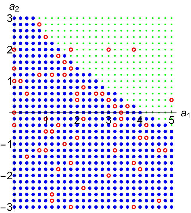
Figure 1: Stability and stationarity solutions of the 3HDM Higgs potential, varying the two quartic parameters $a_{1}$ and $a_{2}$ of the potential (8). The other quartic parameters are set to $a_{3}=-5$, $a_{4}=-0.0474$, $a_{5}=1.5$, $a_{6}=2$, $a_{7}=3$. The quadratic parameters are fixed by the equations (15), the vacuum expectation value $v_{0}$, and the ratio $v_{1}/v_{2}=m_{\mu}/m_{\tau}$ as well as $v_{3}=v_{0}/\sqrt{2}$. The larger full circles (blue) show points where the potential is unstable. The open circles (red) show parameters where no correct electroweak symmetry breaking appears or the vacuum expectation value $v_{0}$ is unequal to 246 GeV. Finally, the small dots (green) have a viable global minimum corresponding to the correct vacuum expectation value.

In case this solution originates from the set (24), that is, when we do have electroweak symmetry breaking $SU(2)_{L}\times U(1)_{Y}$ $\to$ $U(1)_{em}$ , we can directly calculate the vacuum-expectation value of this minimum, $v_{0}^{2}=\sqrt{6}K_{0}$, and verify that it coincides with (16).

Depending on the variation of the parameters $a_{1}$ and $a_{2}$ we detect the viable global minima. These cases are marked by little (green) dots in Fig. 1. In case the deepest potential value does not correspond to the correct electroweak symmetry breaking or does not give the correct vacuum expectation value, these parameter points are denoted by a circle (red) in Fig. 1.

As we can see by the scattering of points, we typically find valid parameters for $a_{1}$ and $a_{2}$ not too small. However, the pattern of valid points appears very sensitive to the parameter values. This, of course, is a consequence of the rather involved potential (8).

Eventually, let us remark on the technical aspects to solve the rather involved systems of equations - on the one hand for the study of stability (20), (21), and on the other hand for the study of stationarity (23), (24). We apply for all the polynomial systems of equations the homotopy continuation approach as implemented in the PHCpack package phcpack . For a brief introduction to the homotopy continuation method, see for instance Maniatis:2012ex .

In the case of the systems of equations (21), (24), we decompose the three component complex vectors $\boldsymbol{w}^{\dagger}$, $\boldsymbol{w}$ into real and imaginary parts. In turn we split every equation in the sets into real and imaginary parts. In this way, all indeterminants in all systems of equations have to be real, and we discard all nonreal solutions. Practically, we treat any solution as real if the imaginary part of any of the inderminants has an amount smaller than 0.001.

Let us study some details of the potential in case it has the correct electroweak symmetry breaking $\mbox{$SU(2)_{L}\times U(1)_{Y}$}\to\mbox{$U(1)_{em}$}$. This is conveniently done in a new basis

$$\varphi_{i}^{\prime}(x)=U_{ij}\varphi_{j}(x),\quad i,j\in\{1,2,3\}$$ (26)

in which only the field $\varphi_{3}^{\prime}(x)$ gets a nonvanishing vacuum expectation value $v_{0}/\sqrt{2}$. The unitary matrix $U$ is determined by two rotation angles, which have to fulfill

$$\begin{split}&v_{1}=\sin(\beta_{2})\sin(\beta_{1})v_{0},\\ &v_{2}=\sin(\beta_{2})\cos(\beta_{1})v_{0},\\ &v_{3}=\cos(\beta_{2})v_{0}\end{split}$$ (27)

with $\beta_{1}\in[0,2\pi[$, $\beta_{2}\in[0,\pi]$ and we have in particular $v_{1}^{2}+v_{2}^{2}+v_{3}^{2}=v_{0}^{2}$. In the new basis, the bilinear parameter vector $(\xi_{\alpha})$ from (13) becomes

$$(\xi_{\alpha}^{\prime})=\begin{pmatrix}\xi_{0}\\ \cos(2\beta_{1})\cos(\beta_{2})\xi_{1}\\ 0\\ \sin(\beta_{1})\cos(\beta_{1})(1+\cos^{2}(\beta_{2}))\xi_{1}+\sqrt{3}/2\sin^{2}(\beta_{2})\xi_{8}\\ -\cos(2\beta_{1})\sin(\beta_{2})\xi_{1}\\ 0\\ \sin(\beta_{2})\cos(\beta_{2})(\sin(2\beta_{1})\xi_{1}-\sqrt{3}\xi_{8})\\ 0\\ \sqrt{3}\cos(\beta_{1})\sin(\beta_{1})\sin^{2}(\beta_{2})\xi_{1}+\frac{1}{4}(1+3\cos(2\beta_{2}))\xi_{8}\end{pmatrix}$$ (28)

The correct global minimum has, in terms of these parameter components, the potential value

$$\langle V\rangle=\frac{v_{0}^{2}}{2\sqrt{6}}\left(\xi^{\prime}_{0}-\sqrt{2}\xi^{\prime}_{8}\right).$$ (29)

This result serves as a good cross-check of the numerical study. In particular, the potential value at vacuum has to be nonpositive in order not to lie above the unbroken minimum, which is given by a vanishing potential.

The physical Higgs bosons follow from the diagonalization of the charged and neutral squared Higgs mass matrices. The neutral field of the third Higgs boson $\varphi_{3}$, that is, $h^{0}(x)$, is a mass eigenstate if the parameters fulfill

$$\xi^{\prime}_{4}=\xi^{\prime}_{5}=\xi^{\prime}_{6}=\xi_{7}^{\prime}=0.$$ (30)

Therefore with a view on (28), we find the explicit conditions for the $O(2)\otimes\mathbbm{Z}_{2}$ model, where the neutral component $h^{0}(x)$ is aligned with the vacuum expectation value. The mass squared of the neutral component is in this case

$$m_{h^{0}}^{2}=\frac{4}{\sqrt{3}}\big{(}\xi^{\prime}_{8}-\frac{1}{\sqrt{2}}\xi^{\prime}_{0}\big{)}.$$ (31)

Alignment thus requires that either $v_{1}=v_{2}$ or $\mu_{m}=0$ which is not the case, since the ratio of the two vacuum expectation values $v_{1}$ and $v_{2}$ is fixed by the ratio of the muon and tau masses, and a nonvanishing parameter $\mu_{m}$ is required in order to break the $O(2)\otimes\mathbbm{Z}_{2}$ symmetry softly.

Let us comment on the neutrino mixing angles $\theta_{13}=0$ and $\theta_{23}=\pi/4$. Since these values seem not to be exactly fulfilled experimentally, we mention that deviations may be achieved by imposing further soft-breaking terms in the potential (8). We have seen that the value and the nature of the global minimum is rather sensitive to small changes of the potential. Therefore, we expect that definite results would require a separate study of the changed potential. However, since additional soft-breaking terms do not affect the quartic part of the potential, and, in particular, we have found that for large parts of parameter space stability follows from the quartic terms alone, we expect stability also in the respective cases of a potential imposing additional soft-breaking terms.

We would like to mention that the parameters $a_{2}$, $a_{3}$, and $a_{4}$ couple the neutral boson $h^{0}(x)$ with the other two generations of doublets. In general this may lead to changed phenomenology in Higgs boson production and decay of the $h^{0}(x)$ field. For some investigation of this we refer to Grimus:2008dr . A further detailed study for instance, with respect to a possible enhancement of the $h^{0}(x)$ decay rate into a pair of photons is left for future work.

3 Conclusions

The $O(2)\otimes\mathbbm{Z}_{2}$ model Grimus:2008dr introduces three Higgs-boson doublets accompanied by an appropriate assignment of the elementary particles to irreducible representations of the group. In this way a neutrino mass matrix is generated which corresponds to mixing angles which are close to the experimental measurements. However, even though the symmetry restricts the model, the Higgs potential appears to be rather involved. Nevertheless, the recently introduced methods to study any three-Higgs doublet model Maniatis:2014oza were applied to study the potential in detail. We have investigated stability, the stationary points, and electroweak symmetry breaking of the Higgs potential by solving the corresponding stationary equations, employing polynomial homotopy continuation. The method numerically finds all the isolated complex solutions out of which we have extracted the physical real solutions. We have scanned over a range of values of the potential parameters. As expected, for too low values of the quartic parameters typically an unstable potential is encountered. For parameter values, corresponding to a stable potential, the global minimum was detected. Our study reveals that in this model there are viable parameters corresponding to a stable global minimum with correct electroweak symmetry breaking.

References

- (1) K. A. Olive et al. [Particle Data Group Collaboration], “Review of Particle Physics,” Chin. Phys. C 38, 090001 (2014).
- (2) M. C. Gonzalez-Garcia, M. Maltoni, J. Salvado and T. Schwetz, “Global fit to three neutrino mixing: critical look at present precision,” J. High Energy Phys. 12, 123 (2012) [arXiv:1209.3023 [hep-ph]].
- (3) S. F. King and C. Luhn, “Neutrino Mass and Mixing with Discrete Symmetry,” Rept. Prog. Phys. 76, 056201 (2013) [arXiv:1301.1340 [hep-ph]].
- (4) E. Ma, “Neutrino mass matrix from S(4) symmetry,” Phys. Lett. B 632, 352 (2006) [arXiv:hep-ph/0508231].
- (5) E. Ma, “Neutrino Tribimaximal Mixing from A(4) Alone,” Mod. Phys. Lett. A 25, 2215 (2010) [arXiv:0908.3165 [hep-ph]].
- (6) R. Gonzalez Felipe, H. Serodio and J. P. Silva, “Neutrino masses and mixing in A4 models with three Higgs doublets,” Phys. Rev. D 88, 015015 (2013) [arXiv:1304.3468 [hep-ph]].
- (7) E. Ma, “Neutrino Mixing and Geometric CP Violation with Symmetry,” Phys. Lett. B 723, 161 (2013) [arXiv:1304.1603 [hep-ph]].
- (8) W. Grimus, L. Lavoura, and D. Neubauer, “A light pseudoscalar in a model with lepton family symmetry O(2),” J. High Energy Phys. 07, 051 (2008) [arXiv:0805.1175 [hep-ph]].
- (9) G. Altarelli and F. Feruglio, “Discrete Flavor Symmetries and Models of Neutrino Mixing,” Rev. Mod. Phys. 82, 2701 (2010) [arXiv:1002.0211 [hep-ph]].
- (10) W. Grimus, L. Lavoura, O. M. Ogreid and P. Osland, “A precision constraint on multi-Higgs-doublet models,” J. Phys. G 35, 075001 (2008) [arXiv:0711.4022 [hep-ph]].
- (11) F. Nagel, “New aspects of gauge-boson couplings and the Higgs sector,” Ph.D.-thesis, Heidelberg University (2004).
- (12) M. Maniatis, A. von Manteuffel, O. Nachtmann and F. Nagel, “Stability and symmetry breaking in the general two-Higgs-doublet model,” Eur. Phys. J. C 48, 805 (2006) [arXiv:hep-ph/0605184].
- (13) C. C. Nishi, “CP violation conditions in -Higgs-doublet potentials,” Phys. Rev. D 74, 036003 (2006) [Erratum 76, 119901 (2007)] [arXiv:hep-ph/0605153].
- (14) M. Maniatis and O. Nachtmann, “Stability and symmetry breaking in the general three-Higgs-doublet model,” J. High Energy Phys. 02, 058 (2015) [arXiv:1408.6833 [hep-ph]].
- (15) J. Verschelde, “Algorithm 795: PHCpack: A General Purpose Solver for Polynomial systems by Homotopy Continuation,” ACM Trans. Math. Software, 25, 2 (1999).
- (16) M. Maniatis and D. Mehta, “Minimizing Higgs Potentials via Numerical Polynomial Homotopy Continuation,” Eur. Phys. J. Plus 127, 91 (2012) [arXiv:1203.0409 [hep-ph]].