Dynamics of the impurity screening cloud following quantum quenches of the Resonant Level Model

Abstract

We present a detailed analysis of the evolution of impurity screening cloud in the Resonant Level Model (RLM) followed by quenches of system parameters. The considered quenches are either local or found to be effectively local. The screening cloud is characterized by impurity-bath correlators and by the entanglement of a block centered around the impurity with the rest of the system. We consider several local quench protocols, such as, quenches from initially decoupled to coupled impurity, quenches between different finite couplings of the impurity, and ‘detuning quenches’ involving changing the onsite impurity potential away from or to the chemical potential of the bath. The relevant correlators and the entanglement display versions of the ‘light-cone’ effect, since the information about the quench travels through the bath at finite speed. At long times (‘inside’ the light cone), the impurity screening cloud relaxes exponentially to the final equilibrium structure, with the relaxation rate given by the emergent energy scale of impurity screening. Also, snaphots of the time-evolving spatial profile of impurity-bath correlators show exponential dependences on space, with the length scale given by the screening length.

1 Introduction

The study of real-time evolution of many-body quantum systems driven out of equilibrium is a subject of intense current interest, partly motivated by remarkable experimental advances in the control of non-equilibrium conditions, both in cold atomic systems and solid-state setups. As a result of this interest, many systems and phenomena in condensed matter physics are being re-examined in non-equilibrium situations. Quantum impurity problems have long been a central paradigm in the study of correlated quantum matter. Impurity models have contributed to influential physical ideas, such as the Kondo model to the development of the renormalization group and the Caldeira-Legget model to the study of decoherence. Quantum impurity models continue today to be a source of new physical insights, and appear in a variety of contexts.

It is therefore not surprising that the study of impurity physics out of equilibrium is attracting an increasing amount of attention. Much work has by now been done on transport through impurities. More relevant to the present work is the interest in real-time dynamics induced by sudden changes (quantum quenches) of impurity Hamiltonians [3, 1, 2, 4, 14, 15, 11, 10, 9, 12, 16, 17, 18, 7, 6, 5, 8, 13].

Generally, an impurity model involves a zero-dimensional object, often a single site or spin, coupled to a bath. The spatial structure of the bath is ignored in much of the literature, but this is exactly the aspect that will concern us in this work: namely the appearance of a spatial signature of the impurity in the bath. This is the so-called ‘impurity screening cloud’. Single-impurity models often possess an emergent energy scale. The most famous is the celebrated Kondo temperature for the single-impurity Kondo model [19, 20], but similar energy scales appear in the single-impurity Anderson model [20, 21, 22] and the interacting resonant level model [23, 24]. There is a length scale $\xi$ corresponding to this energy scale, which suggests that the bath surrounding the impurity is affected differently at distances less than $\xi$ from the impurity than at larger distances $x>\xi$, i.e., there should be a ‘screening cloud’ of radius $\xi$ surrounding the impurity. Although the impurity screening cloud is difficult to observe directly experimentally, calculations have shown that this impurity lengthscale does in fact appear in real-space properties of the bath. The properties (e.g., persistent current or conductivity) of a mesoscopic device containing a Kondo or Anderson impurity have been found to behave differently if the device size is larger or smaller than the size of the Kondo cloud [25, 26, 27, 28, 29]. Numerical and variational calculations have found real-space properties (e.g., impurity-bath correlation functions, distortion of local density of states, entanglement properties, etc) to be different for $x<\xi$ and $x>\xi$ [30, 31, 32, 33, 34, 35, 36, 37, 39, 40, 38], for Anderson and Kondo models and for spin-chain versions of the Kondo model. These recent results extend earlier perturbative calculations of real-space structure [41, 42, 43].

Perhaps the simplest example of an impurity generating a spatially extended screening cloud is that of the resonant level model (RLM), which is a model of non-interacting spinless fermions. A single ‘impurity’ site (or level) is weakly tunnel-coupled to a fermionic bath. The impurity coupling $J$ generates a small energy scale $\Gamma\propto J^{2}$, and a corresponding large length scale $\xi\propto J^{-2}$. The structure of the equilibrium screening cloud in this model was examined in detail in Ref. [44]. The screening cloud was characterized primarily through the two-point correlation function between the impurity site and bath positions at distance $x$ from the impurity. This impurity-bath correlation was found to have different spatial dependence within ($x<\xi$) and outside ($x>\xi$) the cloud. The screening cloud was also described using the entanglement of a spatial block containing the impurity with the rest of the bath; the dependence of this entanglement on the distance of the block boundary from the impurity is different when this distance is smaller than or larger than $\xi$.

In this work, we examine the non-equilibrium response of the screening cloud of the RLM after a quantum quench. We start with quenches of the impurity tunnel coupling $J$ (section 3). This being a local quench, the effect of this change propagates through the bath at a finite speed, and after the ‘wavefront’ has passed through a certain point, observables related to that position relax to the value corresponding to the ground state of the final Hamiltonian. We show that the relaxation of the impurity-bath correlator happens exponentially, with the rate of the exponential decay given by the final impurity screening energy scale $\Gamma_{f}\propto J_{f}^{2}$. At any instant, the deviation of the correlators from their final value is found to increase exponentially with distance from the impurity, with the spatial length scale $\xi$. The space- and time-dependence of the correlators happens largely, but not completely, through the combination ${\Gamma_{f}}t-x/\xi$. For quenches starting from the impurity-decoupled case, we can explain many features of the time evolution of impurity-bath correlators from an analytic calculation in the wide-bandwidth approximation. The evolution of the block entanglement also shows numerical signatures of the screening energy scale $\Gamma_{f}$, in a somewhat more complicated manner. Quenches of the impurity energy (detuning from the bath chemical potential, section 4) results in similar overall behavior as long as the detuning is moderate. If the final detuning is nonzero, this provides an additional oscillation frequency in the dynamics. Finally, we consider a class of global quenches of bath parameters (section 5), and show how these are equivalent to local quenches for the purposes of screening cloud relaxation.

In the concluding section we provide some discussion and context, and contrast several recent studies [3, 2, 1] which are related in spirit to this work.

2 Model, tight-binding realization, and equilibrium properties

We consider the resonant level model (RLM), given by the Hamiltonian

$$H=\sum_{k}\varepsilon_{k}c_{k}^{\dagger}c_{k}~{}+~{}\varepsilon_{d}d^{\dagger}d~{}-~{}J(d^{\dagger}c_{x=0}+c_{x=0}^{\dagger}d)\ .$$ (1)

Here $c_{k}$, $c_{k}^{\dagger}$ ($c_{x}$, $c_{x}^{\dagger}$) are the bath fermion operators at momentum $k$ (at position $x$) and $d$, $d^{\dagger}$ are the fermion operators at the impurity site, $\varepsilon_{k}$ is the dispersion of the bath fermions, and $J$ is the hopping strength between the impurity and position $x=0$ of the bath. The on-site detuning potential $\varepsilon_{d}$ is generally tuned to the bath chemical potential, except in Section 4. Here $x$ represents the distance from the impurity. The impurity coupling $J$ is assumed to be much smaller than the bandwidth of the dispersion $\varepsilon_{k}$; this is the regime where the physics is relatively insensitive to details of the bath dispersion.

At equilibrium, the RLM for small $J$ displays a screening cloud, as examined in detail in Ref. [44]. The details depend weakly on the nature of the bath; we will concentrate on a one-dimensional bath. Specifically, we will use a closed tight-binding chain with $2L-1$ sites, labeled as $x=-(L-1),\ldots,-1,0,1,\ldots,(L-1)$, as shown in Figure 1(a). We will mostly work with nearest-neighbor (n.n.) hopping in the bath, so that the Hamiltonian is

$$H=-\sum_{i=-L+1}^{L-1}(c_{i}^{\dagger}c_{i+1}+c_{i+1}^{\dagger}c_{i})~{}+~{}\varepsilon_{d}d^{\dagger}d~{}-~{}J\left(c_{0}^{\dagger}d~{}+~{}d^{\dagger}c_{0}\right).$$ (2)

The site label $L$ is identified with site $-L+1$ as usual for periodic boundary conditions. We take the bath n.n. hopping to be unity, so that energies (time) is measured in units of the bath n.n. hopping strength (inverse of the bath n.n. hopping strength). The dispersion is then $\epsilon_{k}=-2\cos{k}$, with $k=2\pi{n}/(2L-1)$ and $n=-L+1,...,L-1$. In Section 5, we also modify the bath by adding next-nearest-neighbor hoppings to the tight-binding chain. We will also mostly consider half-filling, i.e., $L$ particles, since the total system including the impurity has $2L$ sites. The bandwidth in these units is $4$, we are thus interested in the parameter regime $J\ll 4$. In practice, we will restrict the final $J$ values to be $\lesssim 0.5$.

The equilibrium screening cloud around the impurity is well described by the single particle impurity-bath correlator $\langle{d^{\dagger}c_{x}}\rangle$ [44]. The zero-temperature equilibrium spatial structure of $\langle{d^{\dagger}c_{x}}\rangle$ features a rapid oscillatory behaviour with wavelength given by the Fermi momentum $k_{F}$, convoluted with an envelope function that crosses over from a $\propto{\rm ln}~{}x$ behaviour at small $x$, to an algebraic decay $\propto x^{-1}$ at large $x$. The length scale $x\sim\xi$ at which this crossover happens, i.e., the ‘size’ of the impurity screening cloud, is $\xi=v_{F}/\pi J^{2}\rho(\varepsilon_{F})$, scaling as $J^{-2}$ with the impurity-bath coupling. Here $v_{F}$ the Fermi velocity and $\rho(\varepsilon_{F})$ the normalized single-particle density of states [$\int d\omega\rho(\omega)=1$] of the bath at the Fermi energy $\varepsilon_{F}$. With our units, at half-filling $v_{F}=2$ and $\rho(\varepsilon_{F})=1/(2\pi)$, so that $\xi=4/J^{2}$.

In Ref. [44], the equilibrium screening cloud was also characterized through a study of the entanglement entropy, motivated by similar characterizations in Refs. [39, 40, 45]. For this purpose, one considers the entanglement entropy $S_{J}^{[\ell]}=-\mathrm{Tr}_{A_{\ell}}[\rho_{A_{\ell}}\ln\rho_{A_{\ell}}]$ of the subsystem $A_{\ell}$ of total size $2\ell$ centered around (and containing) the impurity. Here $\rho_{A_{\ell}}$ is the reduced density matrix of the subsystem $A_{\ell}$ obtained by tracing out the degrees of freedom lying outside the subsystem, starting from the wavefunction (in this case the ground state wavefunction) of the full system. The so-called impurity entropy, defined as

$$S_{imp}^{[\ell]}=S_{J}^{[\ell]}-S_{J=0}^{[\ell]},$$ (3)

was shown to have, as a function of the subsystem size $\ell$, a crossover to a an algebraic $\propto\ell^{-1}$ decay at large $\ell$ around the same characteristic length scale $\xi$ [44].

In the following we analyse the non-equilibrium dynamics of the screening cloud after a quantum quench by monitoring the evolution of $\langle{d^{\dagger}c_{x}}\rangle$ and $S^{[\ell]}$ as a function of time. For a system initialised in the ground-state of the Hamiltonian for $t<0$, we consider local quenches, where either $J$ or $\varepsilon_{d}$ are changed abruptly at $t=0$ to their final values, and also a quench in the global parameters corresponding to an abrupt change of the dispersion relation $\varepsilon_{k}$ of the bath. For a bath with an infinite number of degrees of freedom, local correlators are expected to relax to the local equilibrium values for asymptotic long times after a local quench. For these cases we analyse the way the new equilibrium form of the screening cloud is reached.

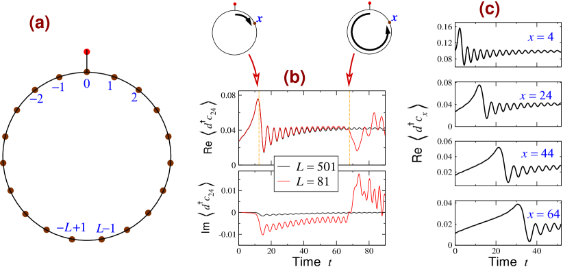
Figure 1: (a) Geometry of tight-binding model (2). (b) Typical behavior of real and imaginary parts of $\langle{d^{\dagger}c_{x}}\rangle$ at $x=24$, after a quench from $J=0.8$ to $J=0.3$. The two dashed vertical lines and the associated cartoons indicate the time for the wavefront to reach the point x ($\sim{x/2}$), and the time for finite-size effects ($\sim\frac{2L+1-x}{2}$). (c) The propagating wavefront, seen visually by comparing the time evolution of $\langle{d^{\dagger}c_{x}}\rangle$ for different $x$.

3 Quenches of the impurity coupling $J$

In this section we will consider quenches of the impurity-bath coupling $J$. The system starts in the ground state for $J=J_{i}$ and, after the $J_{i}\to J_{f}$ quench, evolves under the final Hamiltonian with $J=J_{f}$. In subsections 3.1, 3.2, 3.3, we consider the evolution of the equal-time impurity-bath correlation function

$$C(x,t)=\left\langle d^{\dagger}(t)c_{x}(t)\right\rangle.$$ (4)

In subsection 3.4 we consider the evolution of the block entanglement entropy.

3.1 Time evolution of impurity-bath correlators: general features

In figures 1(b) and 1(c) we display some general features of the time evolution of the impurity-bath correlator, highlighting effects of locality, information propagation, and the appearance of infinite-size quench features in finite-size systems.

After a local quench, information about the change in the system should propagate out from the point of disturbance with speed $v_{F}$. This effect has been discussed widely in recent times in terms of the so-called Lieb-Robinson bound and the ‘light-cone’ effect, for both local and global quenches [46, 47, 48, 3, 1, 2, 56, 55, 54, 53, 52, 51, 50, 49, 57, 58]. For local quenches, one typical way of formulating this causality effect is that a local observable at position $x$ will be substantially affected by a local quench at position $y$ only in the space-time region $t>|x-y|/v$ (‘inside’ the light cone). Here $v$ is the characteristic speed.

The equal-time impurity-bath correlator $C(x,t)=\langle{d^{\dagger}c_{x}}\rangle$ is not a local observable. Thus, it evolves in time also outside the light cone, $t<x/v_{F}$, but this part of the dynamics is entirely due to the $d$ operator and hence relatively simple. The dynamics is dramatically affected at $t\sim{x/v_{F}}$, when the ‘wavefront’ reaches the point $x$. This is shown in the examples of Figure 1(b), in particular the top left schematic. The panels in Figure 1(c) visually display the increasing time required for the wavefront or signal to reach farther points.

Within the light-cone, i.e., for $t>{x/v_{F}}$, the correlator decays approximately (upto $\sim{L}^{-1}$ effects) toward its final ground-state value, $C_{f}^{\rm Eq}(x,t)$. The reasoning behind this is that a local quench is a ${L}^{-1}$ effect and therefore does not inject a thermodynamically significant energy into the system, hence a large enough system should relax approximately to its ground state. Figure 1(b) also shows that finite-size effects are strongly felt when the signal or wavefront traverses the other end of the system and then reaches point $x$ (top right schematic). Until this point of time, $t\approx(2L-x)/v_{F}$, the correlator $\langle{d^{\dagger}c_{x}}\rangle$ is approximately $L$-independent, thus by analyzing this region we essentially access the behavior of $\langle{d^{\dagger}c_{x}}\rangle$ in an infinite system. By increasing the ring size $L$, we get larger windows of time where the infinite-system dynamics can be accessed.

The details of the dynamics depend sensitively on the parameters, filling, and the site $x$. Even for the half-filling case (where the behavior is cleanest, also in equilibrium), the real and imaginary parts of $C(x,t)$ show different dynamics for odd and even $x$. For all $x$, the imaginary part starts from zero and (for large enough systems) goes to zero at long times. For even distances $x$, e.g., Figure 1(b), the imaginary part shows strong finite-size effects and for large enough systems is almost time-independent. For odd $x$ (not shown), the behavior is reversed: $\mathrm{Re}[C(x,t)]$ shows strong $L$-dependence while $\mathrm{Im}[C(x,t)]$ does not. In order to avoid these system- and $x$-dependent details, we will mostly show absolute values, $|C(x,t)|$ or $|C(x,t)-C_{f}^{\rm Eq}(x,t)|$.

A local quantity such as $\langle{c^{\dagger}_{x}c_{x}}\rangle$ or $\langle{c^{\dagger}_{x}c_{x+1}}\rangle$ shows a clearer light-cone effect, i.e., stays constant for $t<{x/v_{F}}$ until the wavefront reaches $x$. Such data is not shown in this work, as our focus is the impurity screening cloud, which is better embodied in the impurity-bath correlator $C(x,t)=\langle{d^{\dagger}c_{x}}\rangle$. Also, Ref. [1] has discussed the appearance or absence of the light-cone effect in different unequal-time correlators.

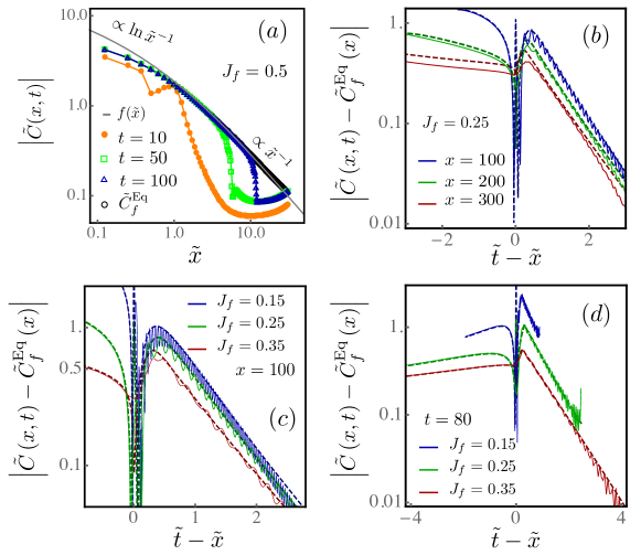
Figure 2: Quenches from an initially decoupled impurity ($J_{i}=0$). The solid lines are tight-binding numerical results for sizes $L\simeq 1000$. Dashed lines are the infinite-bandwidth infinite-size results of Eq. (7). (a) Snapshots of the rescaled impurity-bath correlation function $\tilde{C}(x,t)$ as a function of $\tilde{x}=x/\xi_{f}$ for different times. $f(\tilde{x})$ is the scaling function obtained in Ref. [44]. (b,c) Time evolution of the difference between $\tilde{C}(x,t)$ and its equilibrium value $\tilde{C}_{f}^{{Eq}}(x)$, at several positions $x$. We plot against the rescaled and shifted time variable $\tilde{t}-\tilde{x}$. (d) Snapshots of the spatial profile of $\left|\tilde{C}(x,t)-\tilde{C}_{f}^{{Eq}}(x)\right|$ at time $t=100$.

3.2 Starting from decoupled impurity: $J_{i}=0$

We first consider an initially decoupled impurity level which is suddenly coupled at time $t=0$ by changing the impurity hopping parameter $J$ from $J_{i}=0$ to finite $J_{f}$. The initial correlation functions are thus given by

$$\langle{c_{k}^{\dagger}c_{k^{\prime}}}\rangle_{0}=\delta_{kk^{\prime}}\Theta(k_{F}-|k|);\quad\langle{d^{\dagger}d}\rangle_{0}=n_{d};\quad\langle{d^{\dagger}c_{x}}\rangle=0$$ (5)

where $n_{d}$ is the initial occupancy of the impurity level. In the final equilibrium state, with $J=J_{f}\neq 0$, the impurity is screened over a finite distance $\xi_{f}=v_{F}/\Gamma_{f}$, with $\Gamma_{f}=\pi J^{2}_{f}\rho(\varepsilon_{F})$.

In these conditions the evolution of the equal-time two-point correlator $\langle{d^{\dagger}(t)c_{i}(t)}\rangle$ is amenable to an analytic treatment along the same lines of Ref. [1]. The approach is detailed in the Appendix. We will express results in terms of the rescaled correlator

$$C(x,t)=\frac{J}{\pi^{2}v_{F}}\tilde{C}(x,t)\,.$$ (6)

In the thermodynamic limit and the large-bandwidth limit, we obtain the following expression for the time evolution of the rescaled impurity-bath correlator:

$$\tilde{C}(x,t)=\pi\int_{-\infty}^{0}d\varepsilon\frac{\left[1-e^{-i(\varepsilon-i)\tilde{t}}\right]\cos\left[\tilde{x}\left(\varepsilon+\tilde{k}_{F}\right)\right]}{(\varepsilon-i)}$$

$$~{}-~{}\theta(\tilde{t}-\tilde{x})\left[i\pi e^{ik_{F}x}\right]\int_{-\infty}^{0}\frac{d\varepsilon e^{i\varepsilon\tilde{x}}}{\varepsilon^{2}+1}\left[1-e^{-i(\varepsilon-i)\tilde{t}}\right]\left[1-e^{i(\varepsilon+i)(\tilde{t}-\tilde{x})}\right]\,.$$ (7)

Here $\tilde{x}=x/\xi_{f}$, $\tilde{t}=\Gamma_{f}{t}$, and $\tilde{k}_{F}=\xi_{f}k_{F}$ are dimensionless versions of distance, time and Fermi momentum, obtained by scaling with the length scale $\xi_{f}$ and energy scale $\Gamma_{f}$ of the impurity screening cloud corresponding to the final impurity coupling $J_{f}$. For our lattice Hamiltonian (2) at half-filling, $k_{F}=\pi/2$.

We comment on several features in this expression:

• There is a clear and natural separation between behaviors for $\tilde{t}<\tilde{x}$ and for $\tilde{t}>\tilde{x}$, i.e., inside and outside the light cone. The first term shows that the evolution is not frozen for $\tilde{t}<\tilde{x}$ (outside the light-cone). As discussed in the previous section, this is expected in the impurity-bath correlator because of the evolution of the impurity operator $d^{\dagger}(t)$

• The impurity screening cloud (associated with the ground state of the final Hamiltonian) sets time- and length- scales for some of the dynamics, since time and position appear in the combinations $\tilde{t}=\Gamma_{f}{t}$ and $\tilde{x}=x/\xi_{f}$ in the expression. In particular, the non-oscillatory part of the time-dependence factorizes out of the integrals and is of the form $e^{-\tilde{t}}$, which shows that the long-time decay to the final value is exponential in time with time constant $1/\Gamma_{f}$.

• The time-dependent correlator displays $k_{F}$ oscillations in space, due to factors like $e^{ik_{F}x}=e^{i\tilde{k}_{F}\tilde{x}}$, just like the equilibrium behavior of the correlator [44].

• In the $\tilde{t}>\tilde{x}$ part (inside the light-cone), a non-oscillatory exponential spatial dependence $~{}e^{\tilde{x}}$ can be factored out of the integral. Thus, the deviation from the final equilibrium value increases exponentially with distance, in the spatial region in which the wavefront has already propagated through.

• The long-time limit ($t\to\infty$) of this expression reduces to the equilibrium expression for the impurity-bath correlator derived in Ref. [44], showing that for large sizes the impurity-bath correlator reduces to the final equilibrium profile.

• There are no temporal oscillations with frequency $=2$ (twice the bath hopping or half the bath bandwidth). In calculations with the tight-binding model 2, oscillations at this frequency appear, as in Figure 1(b,c); this represents the energy width of occupied single-particle states. However, since the expression is obtained in the infinite-bandwidth limit, the bandwidth or hopping parameter of the bath do not appear as an oscillation time-scale.

Figure 2 shows the impurity-bath correlation function $\tilde{C}(x,t)$ after quenches starting from the decoupled case, $J_{i}=0$, comparing numerical tight-binding results using Hamiltonian (2) against predictions from Eq. (7) above derived in the large-size large-bandwidth limit.

Figure 2(a) shows snapshots of the spatial profile of $|\tilde{C}(x,t)|$, calculated for the tight-binding Hamiltonian at different time instants $t$ after the quench. The spatial profile is seen to approach the final equilibrium curve at large times. The (final) equilibrium profile approximates the analytic equilibrium curve $f(\tilde{x})$, but does not match it exactly for a single finite system size and single $J_{f}$ value, as discussed in detail in Ref. [44].

To highlight the approach to equilibrium, in Figures 2(b,c,d) we show the correlator with the final equilibrium value subtracted off, i.e, $\tilde{C}(x,t)-\tilde{C}_{f}^{{Eq}}(x)$. Motivated by the light-cone structure, we plot this as a function of the variable $\tilde{t}-\tilde{x}$. The behavior outside the light-cone ($\tilde{t}<\tilde{x}$) and inside the light-cone ($\tilde{t}>\tilde{x}$) look sharply different in this quantity. The quantity is plotted for different bath positions $x$ (Figure 2(b)), and for different final coupling $J_{f}$ at the same bath position $x=100$ (Figure 2(c)). In the log-linear plots, the decay for $\tilde{t}>\tilde{x}$ appear as straight lines with the same slope in each of these cases, showing that the decay to the final value inside the light cone happens exponentially with the time scale associated with the (final) impurity screening cloud.

Figure 2(d) plots spatial snapshots of the correlator at the same time instant, $t=100$. We choose to plot it against the same variable $\tilde{t}-\tilde{x}$ used for showing the time evolution in Figures 2(b,c). The similarity of panel 2(d) with the plots in 2(b,c) highlights the fact that the dynamical features are dominanted by the quantity $\tilde{t}-\tilde{x}$. In Figure 2(d) we clearly see an exponential increase of the deviation from the final value, with increasing distance. This is consistent with the $e^{\tilde{x}}$ factor in the infinite-bandwidth expression, discussed above. There are small $e^{ik_{F}x}$ oscillations, but they are negligible everywhere except at small values of $x$. These oscillations appear in both the tight-binding data and in the infinite-bandwidth equation, and show strong finite-size effects.

In each panel of Figure 2, we show tight-binding results (solid curves) together with the prediction Eq. 7 (dashed curves). For the regime under discussion, the infinite-bandwidth continuum approximation captures well the essential features of the impurity cloud dynamics as seen through the $C(x,t)$ correlator. The agreement is generally excellent. Points of disagreement are the temporal oscillations of frequency 2 (half the bandwidth) appearing in the lattice data but not in the infinite-bandwidth analytics, and the difference between the $e^{ik_{F}x}$ oscillations, which are anyway very small.

3.3 Quench from finite $J_{i}$ to finite $J_{f}$

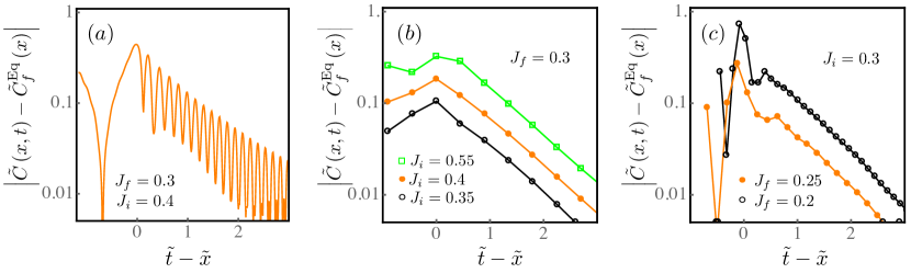
Figure 3: Quenches from finite $J_{i}$ to finite $J_{f}$. (a) Relaxation of the impurity-bath correlation function, for $x=50$. In (b,c), the results are averaged over small time intervals $\Delta{t}$ to average out the strong oscillations and emphasize the exponential decay with rate $\Gamma_{f}$. In panels (b) and (c), $\Delta{t}=20$ and $\Delta{t}=12$ respectively.

We now consider quenches from finite $J_{i}\neq 0$ to a different finite value $J_{f}$. The initial correlators now no longer have a simple form like Eq. (5) for the $J_{i}=0$ case, but rather they describe a screening cloud with characteristic length $\xi_{i}\propto{J_{i}}^{-2}$.

After the quench, the correlator $C(x,t)$ relaxes in an analogous way to the new equilibrium profile corresponding to the length $\xi_{f}\propto{J_{f}}^{-2}$. As the light cone spreads, $C(x,t)$ within the light cone ($x<v_{F}t$) at time $t$ will relax exponentially to the final profile.

In principle, an integral expression for the correlation function $C(x,t)$ could be derived analytically using a similar method to the one given in the appendix for $J_{i}=0$. However, such an expression would involve additional integrals, because the initial $C(x,0)$ is already nontrivial [44]. We therefore restrict to showing numerical results from the tight-binding model. For $J_{i}\neq 0$, the temporal oscillations of $C(x,t)$ (with frequency $\varepsilon_{F}$) are much stronger than in the $J_{i}=0$ case, as seen in Figure 3(a). To focus on the exponential relaxation, in Figures 3(b) and 3(c) we average out the oscillations by plotting the running average of $C(x,t)$, i.e., each point is an average of $C(x,t)$ taken over a small time window $\Delta t$ around time $t$. For a variety of $J_{i}$ and $J_{f}$ values, the relaxation is seen to be always exponential, with the time scale corresponding to the final impurity screening scale $\Gamma_{f}=\pi J^{2}_{f}\rho(\varepsilon_{F})$.

3.4 Entanglement entropy

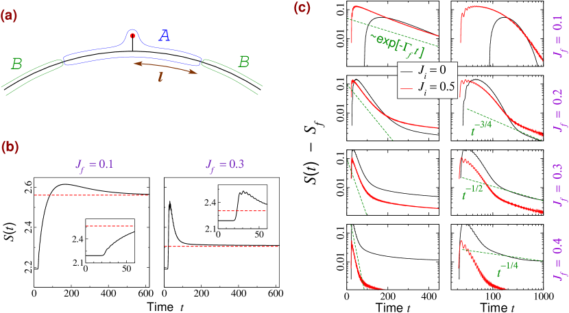
Figure 4: (a) Geometry for defining block entanglement between $A$ and $B$ partitions. (b) Time evolution of entanglement entropy, with $l=40$, after a quench from $J_{i}=0$ to two different final $J_{f}$. The dynamics starts at $t=l/v_{F}=20$, after the signal reaches bourndary between $A$ and $B$ blocks. The insets zoom around this instant. The dynamics clearly is faster for larger $J_{f}$. The entanglement entropy approaches the final ground-state value (dashed horizontal lines) at long times. (c) Effect of $J_{f}$ on the relaxation explored in detail, for quenches starting from $J_{i}=0$ and from $J_{i}=0.5$. The left panels (log-linear scale) highlight the initial ${\sim}e^{-\Gamma_{f}t}$ behavior. The right panels (same data, log-log scale) show that the long-time behavior is an approximate power law, with drifting exponent that suggests a logarithmic correction as in Ref. [59].

We now consider the time evolution of the entanglement entropy $S^{[\ell]}(t)$ between a block $A$ containing the impurity at the center, and the rest of the system, which we call $B$. The geometry is shown in Figure 4(a). The block $A$ contains a total of $2\ell$ sites including the impurity, so that the boundary between the blocks is at distance $\ell$ from the impurity.

The entanglement entropy in a free-fermion system can be obtained from the matrix of all two-point correlators within one of the blocks [60, 59, 44]: if $\nu_{i}$’s are the eigenvalues of this matrix, then $S=-\sum_{i}[\nu_{i}{\rm ln}\nu_{i}+(1-\nu_{i}){\rm ln}(1-\nu_{i})]$. In the present case, we calculate the entanglement $S^{[\ell]}(t)$ at instant $t$ from the matrix of equal-time two-point correlators at time $t$.

Ref. [59] has studied the entanglement evolution after a particular local quench, for a block containing the quench position at the center. (The strength of a single bond of the chain is quenched.) The results are intriguing and, to the best of our knowledge, not yet completely understood: the block entanglement entropy decays to the final equilibrium value with a power law modified logarithmically. This is accompanied by $\ln{t}$ behaviors of some of the eigenvalues $\nu_{i}$ of the correlation matrix. Our situation is broadly similar, but we are particularly interested in the role of the impurity screening scale in the dynamics.

Figure 4(b) shows the behavior of $S^{[\ell]}(t)$ after a quench starting at $J_{i}=0$. (The overall behavior for other $J_{i}$ values is very similar.) The entanglement between the blocks stays frozen at the initial value until the information wavefront reaches the boundary between the blocks, i.e., until $t\sim\ell/v_{F}$. This may seem surprising because many correlators in the correlation matrix of $A$ have dynamics at smaller times (as seen in previous sections), but it is physically reasonable because $S^{[\ell]}(t)$ measures the entanglement between $A$ and $B$ blocks, and the $B$ block cannot know about the local quench until this time. After a sharp reaction shortly after $t\gtrsim\ell/v_{F}$, the entanglement relaxes toward the final ground state value, shown in Figure 4(b) with dashed horizontal lines. The overall form of $S^{[\ell]}(t)$ is broadly similar to that seen in the local quench of Ref. [59]. The response and relaxation behavior are clearly faster at larger $J_{f}$, consistent with the fact that the energy scale of the screening cloud ($\Gamma_{f}$) increases with $J_{f}$.

The relaxation behavior is examined in more detail in Figure 4(c). There are two time regimes, separated by a time scale proportional to $\Gamma_{f}\sim{J_{f}}^{2}$. (For $J_{f}=0.1$, only the first regime is visible.) The initial relaxation regime is exponential, with the time constant given by $\Gamma_{f}^{-1}$. This feature is related to the physics of impurity screening and does not appear in the quench of Ref. [59]. At later times, the relaxation is slower; the data for accessible sizes is consistent with a power law but the best-fit exponents vary. This suggests that the exact behavior in this long-time regime may well have logarithmic corrections as in Ref. [59]. The time evolution of the eigenvalues $\nu_{i}$ also shows logarithmic evolution of some eigenvalues as in Ref. [59]; a full understanding is lacking at present, but presumably the $\ln{t}$ features are not related to impurity screening physics.

4 Quenches of the impurity detuning $\varepsilon_{d}$

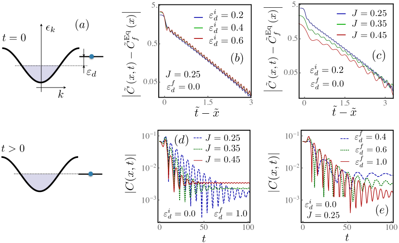
Figure 5: (a) Schematic showing a quench from finite to zero detuning. (b,c) Relaxation of impurity-bath correlators for quenches to zero detuning. (d,e) Evolution of impurity-bath correlators for quenches to finite detuning. In order to compare frequencies, in these panels we plot against time without rescaling.

In this section we study the dynamics after quenching the detuning, i.e., the onsite energy bias of the impurity site, denoted by $\varepsilon_{d}$ in Equations (1) and (2). The detuning energy is measured with respect to the Fermi energy, as shown in Figure 5(a). We consider both quenches from an initially detuned impurity potential to the zero detuning case, $\varepsilon_{d}^{i}\neq 0$ to $\varepsilon_{d}^{f}=0$, and vice versa. The first situation is depicted in Figure 5(a). The impurity coupling $J$ is kept unchanged in this quench protocol.

For the ground state, tuning of the on-site impurity potential changes the structure of the impurity cloud at small distances (within the screening cloud, $x<\xi$) and eventually destroys the logarithmic dependence $\propto{\rm ln}~{}x$ of the correlation function $\langle{d^{\dagger}c_{i}}\rangle$ in this spatial region [44]. However, the effect is significant only at large $\varepsilon_{d}$ [44]. Here, we consider moderate values of $\varepsilon_{d}$, of the order of the bath bandwidth.

Figures 5(b,c) show quenches of the detuning to a final zero value, $\varepsilon_{d}^{f}=0$. The relaxation of correlators to the final ground state value is exponential, with the relaxation rate set by the screening cloud scale, $\Gamma_{f}=J_{f}^{2}/2$, as before. The data shows the usual half-bandwidth frequency oscillations. In Figure 5(c) the oscillation periods appear to be differentfor different $J$, but this is only due to the $J$-dependent scaling of the time axis.

In Figures 5(d,e) we show the dynamics after quenches to $\mathcal{O}(1)$ values of $\varepsilon_{d}^{f}$. The decay to the final values occur exponentially, with the same time scale $\Gamma_{f}$, consistent with the fact that moderate $\varepsilon_{d}^{f}$ values do not destroy the screening cloud [44]. However, there are now strong oscillations with freuquency $\varepsilon_{d}^{f}$. To highlight the frequencies, we use axes without dividing by the screeing scale. The correlators now show oscillations with two frequencies — one equal to half the bandwidth and one equal to $\varepsilon_{d}^{f}$. In Figure 5(d) the new frequency $\varepsilon_{d}^{f}=1$ (prominient oscillations at smaller times) is half that of the smaller oscillations visible at later times. In 5(e) the oscillation frequency visibly varies with $\varepsilon_{d}^{f}$.

At extremely large final detuning values, $\varepsilon_{d}^{f}\gg 1$ (not shown), the relaxation appears to be power-law-like rather than exponential, for accessible system sizes. Since this value is larger than the bandwidth, this is beyond the regime of usual impurity phsyics, and is consistent with the absence of impurity screening.

5 Global quenches with local effects

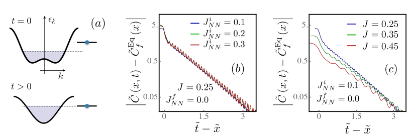
Figure 6: (a) Schematic showing a quench from finite $J_{NN}$ to $J_{NN}=0$. (b,c) Relaxation of impurity-bath correlators, for various quenches ending at $J^{f}_{NN}=0$. Panel (b) uses various initial $J_{NN}$ values and panel (c) uses various $J$ values. The behavior is remarkably similar to the case of detuning quenches.

In this section we consider a global quench which behaves effectively like a local quench, in the sense that the correlators relax to the ground state impurity screening cloud corresponding to the final Hamiltonian. We consider a quench that changes the dispersion of the bath, through a next-nearest neighbor hopping with opposite sign compared to the nearest-neighbor hopping. The Hamiltonian is now

$$H=-\sum_{i=-L+1}^{L-1}(c_{i}^{\dagger}c_{i+1}+c_{i+1}^{\dagger}c_{i})~{}+~{}J_{NN}\sum_{i=-L+1}^{L-1}(c_{i}^{\dagger}c_{i+2}+c_{i+2}^{\dagger}c_{i})$$

$$~{}+~{}\varepsilon_{d}d^{\dagger}d~{}-~{}J\left(c_{0}^{\dagger}d~{}+~{}d^{\dagger}c_{0}\right).$$ (8)

This corresponds to a dispersion relation $\varepsilon_{k}=-2J\cos(k)+2J_{NN}\cos(2k)$, as shown in the top cartoon in Figure 6(a).

The equilibrium (zero temperature) effects of such a modification to the bath dispersion was explored in some detail in Ref. [44]. At any filling fraction, there are three regimes of behavior depending on the value of $J_{NN}$. For half-filling these behaviors are as follows: For $J_{NN}>1$, the bath has two pairs of Fermi points rather than a single pair; the impurity screening cloud has the same form except that the density of states now has contributions from four Fermi points. The $J_{NN}=1$ case is special as there is single Fermi ‘touching’ point instead of a pair of Fermi crossing points. In this case the correlators show a non-Fermi-liquid character for distances exceeding the screening length. Finally, the $0<J_{NN}<1$ regime is very similar to the case of the un-modified bath, with two Fermi points.

In the absence of the impurity, the single-particle Hamiltonian with and without the $J_{NN}$ term has the same eigenstates for each momentum, only the eigen-energies are affected. For any $J_{NN}\in[0,1]$, the same single-particle momenta $k\in[-\frac{\pi}{2},\frac{\pi}{2}]$ constitute the ground-state Fermi sea at half filling, so that an abrupt change of $J_{NN}$ in the absence of an impurity would leave the system stationary and not have any non-equilibrium effects. Such a quench has an effect only due to the presence of an impurity, so that it is effectively a local quench. For present purposes we consider half-filling and $0\leq J_{NN}<1$.

Figure 6 shows data for quenches from nonzero $J_{NN}$ to $J_{NN}=0$, with the detuning parameter set to zero: $\varepsilon_{d}=0$. The initial equilibrium state has two Fermi points as in the case of an un-modified bath; however the chemical potential is no longer at zero for half-filling, so that the detuning compared to the Fermi surface is initially nonzero. Such a quench is thus effectively a detuning quench of the impurity. In fact, the results for the time evolution of impurity-bath correlators shown in Figure 6(b,c) are remarkably similar to those in Figures 5(b,c), where the detuning was quenched from nonzero values to zero. The change in the dispersion modifies $v_{F}$ and $\rho(\varepsilon_{F})$; this also has an effect on the dynamics of impurity-bath correlators, but the dominant effect is clearly the change of detuning between Fermi level and impurity energy.

We have also performed quenches from $J_{NN}=0$ to $J_{NN}>0$ (not shown). Repeating the argument above, these are similar to detuning quenches from zero to nonzero detuning. Accordingly, the time evolution of $C(x,t)=\langle{d^{\dagger}c_{x}}\rangle$ is very similar to the detuning quench results of Figures 5(d,e).

6 Discussion

We have presented a study of the dynamics of the impurity screening cloud in the resonant level model following local (or effectively local) quenches. We have focused mostly on the time-dependence of the equal-time impurity-bath correlators $C(x,t)=\langle{d^{\dagger}(t)c_{x}(t)}\rangle$, which characterizes the screening cloud at equilibrium [44].

Due to the finite speed of propagation in the bath, the effect of the quench is felt at point $x$ only at times $t>x/v_{F}$. In terms of the correlator $C(x,t)$, this means that for $t<x/v_{F}$ the dynamics is due only to the evolution of the $d^{\dagger}$ operator. Thus, $C(x,t)$ has relatively simple evolution for $t<x/v_{F}$. After the information wavefront has passed point $x$, the correlator relaxes to the ground state of the final Hamiltonian, provided the system is large enough. We have outlined how the behavior is modified for finite-size baths, and how the infinite-system quench properties can be extracted from time evolution data on finite-size systems.

The relaxation to the final ground state value is found to happen exponentially, with the rate given by the energy scale $\Gamma_{f}$ associated with impurity screening in the final Hamiltonian. This is the scale of broadening of the impurity spectral function [44], analogous to the Kondo temperature scale in the single-impurity Kondo model. We have highlighted the relaxation with this scale after the wavefront passes the point at time $x/v_{F}$, by plotting $\left|C(x,t)-C_{f}^{Eq}(x)\right|$ against the rescaled and shifted time variable $\Gamma_{f}(t-\frac{x}{v_{F}})=\tilde{t}-\tilde{x}$ for a variety of quenches, with $\Gamma_{f}$ determined by the final impurity coupling $J_{f}$. The relaxation curves plotted in this way look broadly similar for a range of quenches. For the case of a quench starting from $J_{i}=0$, we derived and presented an explicit expression for $C(x,t)$, which analytically expresses these physical effects, e.g., through explicit appearance of $\theta(\tilde{t}-\tilde{x})$ factors signaling the information wavefront.

We have also described the effect of a detuning quench on the equal-time correlators. For moderate detunings, the exponential relaxation persists, and if there is a final nonzero detuning with respect to the chemical potential, this provides an additional oscillation frequency. A quench of the bath involving nearest-neighbor hoppings reduces effectively to a local quech as long as the number of Fermi points is preserved.

The evolution of the entanglement entropy of a block centered around the impurity shows a clear light-cone effect (no dynamics before $t\sim{x}/v_{F}$). For $t>x/v_{F}$, we find two relaxational regimes. The first regime shows exponential relaxation with the rate $\Gamma_{f}$. The longer-time regime is consistent with a power-law relaxation with logarithmic corrections, as in the case of Ref. [59].

The dynamics of impurity screening clouds has been the subject of a few recent studies [3, 2, 1], complementary to ours. We briefly outline relevant parts of these results below and compare with our results.

In Ref. [1], the authors have studied the Kondo model at the so-called Toulouse point [61]. At the Toulouse point, the Kondo model reduces to the non-interacting resonant level model, and hence various analytical results can be derived in the case when one starts from zero coupling. The authors focus on spin-spin correlators of the Kondo model, which translate to different fermionic correlators from the ones occurring naturally in this work. Focusing on unequal-time correlators, Ref. [1] distinguishes correlators which show a strict light cone from those which do not.

In Ref. [2], quenches in the isotropic Kondo model are studied using time-dependent NRG and perturbation theory, for both ferromagnetic and antiferromagnetic Kondo couplings. The time evolution of equal-time impurity-bath spin-spin correlators are studied. As in our case, the correlators considered do not have a strict light cone.

Ref. [3] addresses several issues similar to the ones addressed in the present work. In this work, the dynamics of the Anderson model is studied with a focus on the Kondo regime. Two types of equal-time impurity-bath correlators are studied: spin-spin and density-density correlators. The behavior for $t<x/v_{F}$ and $t>x/v_{F}$ are characterized in some detail, and the exponential decay for $t>x/v_{F}$ is discussed. The decay rate appears to be more complicated than in our case and weakly dependent on position; it is not completely clear whether this is due to system size issues.

The present study has focused on the noninteracting RLM and the dynamics of correlators naturally suitable for describing the RLM screening cloud. The absence of interactions has allowed us to numerically treat relatively large systems, making possible an unambiguous identification of the time scale of relaxation. This aspect is more difficult with sizes accessible for interacting systems [3]. In addition, our analytical result for the $J_{i}=0$ case explicitly shows ${\sim}e^{-\Gamma_{f}t}$ relaxation of the equal-time impurity-bath correlators. Based on the present results, it is natural to conjecture that the relaxation rate is given by the characteristic equilibrium impurity energy scale for any impurity model characterized by an emergent energy scale. For example, the Kondo temperature scale should provide the relaxation rate for the antiferromagnetic Kondo case of Ref. [2], but the details of relaxation are not yet clarified in the literature.

The previous studies concentrate on initially decoupled impurities, i.e., cases where there is no nontrivial screening cloud in the initial state. In section 3.3 we have presented numerical results for finite initial coupling $J_{i}$. Even though the relaxation is governed solely by the final impurity energy scale, the structure of the initial screening cloud induces strong oscillations superposed on the relaxation.

Local quenches are being currently studied from a variety of perspectives. The present work, together with the related literature discussed above, addresses the role of the emergent energy scale in the dynamics, in cases where the local feature possesses such a scale. Several aspects remain poorly understood and clearly deserve further investigation and explanation, such as the behavior of the block entanglement entropy and entanglement spectrum, the role of finite bandwidths, etc.

7 Details of the derivation

Eq. (7), reported in the main text, gives the time evolution of impurity-bath correlators in the infinite-bandwidth and infinite-bath-size limit. In this appendix we briefly outline the derivation of this expression.

The evolution of the system after the quench at time $t=0$ is governed by the final Hamiltonian given in Eq.(1) which in its eigen-operator basis $a_{\varepsilon}$ can be written in the form $H=\sum_{\varepsilon}\varepsilon\,a^{\dagger}_{\varepsilon}a_{\varepsilon}$. The new set of operators $a_{\varepsilon}$, $a_{\varepsilon}^{\dagger}$ can be related with the original $c_{k}$ and $d$ by imposing the commutation relations $\left[H,a_{\varepsilon}\right]=-\varepsilon a_{\varepsilon}$. This yields

$$a_{\varepsilon}=A_{\varepsilon d}d+\sum_{k}A_{\varepsilon k}c_{k},\quad a_{\varepsilon}^{\dagger}=A_{\varepsilon d}^{*}d^{\dagger}+\sum_{k}A_{\varepsilon k}^{*}c_{k}^{\dagger}$$ (9)

with

$$A_{\varepsilon d} = A_{\varepsilon d}^{*}=\sqrt{\frac{2v_{F}}{2L+1}\frac{\Gamma}{\Gamma^{2}+\varepsilon^{2}}},$$ (10)

$$A_{\varepsilon k} = A_{\varepsilon k}^{*}=\frac{J^{\prime}}{\sqrt{2L+1}}\frac{1}{\varepsilon-\varepsilon_{k}}\sqrt{\frac{2v_{F}}{2L+1}\frac{\Gamma}{\Gamma^{2}+\varepsilon^{2}}}$$ (11)

Note that the unitarity of the transformation also implies that

$$c_{k}=\sum_{\varepsilon}A_{\varepsilon k}a_{\varepsilon};\quad d=\sum_{\varepsilon}A_{\varepsilon d}a_{\varepsilon}.$$ (12)

The time evolution of the operators $d^{\dagger}(t)$ and $c_{r}(t)$ can be most easily computed in the basis where $H$ is diagonal. This leads to the expressions:

$$d^{\dagger}(t) = \sum_{\varepsilon}|A_{\varepsilon d}|^{2}e^{i\varepsilon t}d^{\dagger}(0)+\sum_{\varepsilon,k}A_{\varepsilon d}A_{\varepsilon k}e^{i\varepsilon t}c_{k}^{\dagger}(0),$$ (13)

$$c_{x}(t) = \frac{1}{\sqrt{2L+1}}\Bigg{[}\sum_{k,\varepsilon}A_{\varepsilon k}A_{\varepsilon d}e^{ikx}e^{-i\varepsilon t}d(0)$$ (14)

$$+ \sum_{k,k^{\prime},\varepsilon}A_{\varepsilon k}A_{\varepsilon k^{\prime}}e^{ikx}e^{-i\varepsilon t}c_{k^{\prime}}(0)\Bigg{]},$$

relating the time evolved operators to the operators at $t=0$. In order to obtain a useful expression for the correlator $\langle{d^{\dagger}(t)c_{x}(t)}\rangle$, we now introduce two approximations. The first is the thermodynamic limit where an infinite chain is considered. The second is the wide-band approximation where we assume that the energy scales of interest are much smaller than the bandwidth of the chain. This amounts to considering that the density of states of the bath is constant. With these two approximations in place, the summations over momentum can be done assuming a linear dispersion relation around the two Fermi points: $\varepsilon_{k}=v_{F}(k-k_{F})$ and $\varepsilon_{k}=-v_{F}(k+k_{F})$. Thus for any function $f(k)$ of momentum we have:

$$\frac{1}{2L+1}\sum_{k}f(k)\to\int\frac{d\varepsilon_{k}}{2\pi v_{F}}\left[f(k_{F}+v_{F}^{-1}\varepsilon_{k})+f(-k_{F}-v_{F}^{-1}\varepsilon_{k})\right]$$ (15)

However, some of the coefficients of the unitary transformation have denominators of the form $\frac{1}{\varepsilon-\varepsilon_{k}}$ which have to be treated with care when $\varepsilon\simeq\varepsilon_{k}$. By analysing the discrete version of the eigenvalue equation of the $H$:

$$\varepsilon=\frac{J^{2}}{2L+1}\sum_{k}\frac{1}{\varepsilon-\varepsilon_{k}}$$ (16)

one arrives at the prescription (see also Ref.[1] and references therein)

$$\frac{1}{\varepsilon-\varepsilon_{k}}\to P\left(\frac{1}{\varepsilon-\varepsilon_{k}}\right)+\pi\frac{\varepsilon}{\Gamma}\delta\left(\varepsilon-\varepsilon_{k}\right).$$ (17)

where $P$ stands for the principle value. Within the considered approximations, the summations in Eqs.(13, 14) can thus be replaced by integrals and partially done by contour deformation in the complex plane. An example of such a procedure for a typical term arising in the computation of $c_{x}(t)$ is:

$$\frac{1}{\sqrt{L}}\sum_{\varepsilon,k}e^{i(kx-\varepsilon t)}A_{\varepsilon k}A_{\varepsilon d} \simeq \frac{J}{2\pi^{2}}\int d\varepsilon\frac{e^{-i\varepsilon t}}{\varepsilon^{2}+\Delta^{2}}\sum_{s=\pm 1}\int\frac{d\varepsilon_{k}}{2\pi v_{F}}e^{is(k_{F}+v_{F}^{-1}\varepsilon_{k})x}\times$$ (18)

$$\left[{\rm P}\left(\frac{1}{\varepsilon-\varepsilon_{k}}\right)+\pi\frac{\varepsilon}{\Delta}\delta(\varepsilon-\varepsilon_{k})\right]$$

$$= -i\frac{J}{v_{F}}e^{ik_{F}x}\theta\left(\tilde{t}-\tilde{x}\right)e^{-(\tilde{t}-\tilde{x})}$$

where we assumed $x>0$ for simplicity. The pole structure of the expression leads to the theta-function term $\theta(\tilde{t}-\tilde{x})$ in Eq.(7) that signals the passage of the wave front through the rescaled position $\tilde{x}$.

References

References

- [1] Medvedyeva M, Hoffmann A, and Kehrein S, 2013 Phys. Rev. B 88, 094306
- [2] Lechtenberg B and Anders F B, 2014 Phys. Rev. B 90 045117
- [3] Nuss M, Ganahl M, Arrigoni E, von der Linden W, and Evertz H G, 2014 Phys. Rev. B 91, 085127
- [4] Kleine C, Mußhoff J, and Anders F B, 2014 Phys. Rev. B 90, 235145
- [5] Vasseur R, Trinh K, Haas S, and Saleur H, 2013 Phys. Rev. Lett. 110, 240601
- [6] Vasseur R and Moore J E, 2014 Phys. Rev. Lett. 112, 146804
- [7] Kennes D M, Meden V, and Vasseur R, 2014 Phys. Rev. B 90, 115101
- [8] Vinkler-Aviv Y, Schiller A, and Anders F B, 2014 Phys. Rev. B 90, 155110
- [9] Latta C, Haupt F, Hanl M, Weichselbaum A, Claassen M, Wuester W, Fallahi P, Faelt S, Glazman L, von Delft J, Türeci H E, and Imamoglu A, 2011 Nature 474 627
- [10] Schiró M, 2012 Phys. Rev. B 86 161101(R)
- [11] Münder W, Wechselbaum A, Goldstein M, Gefen Y, and von Delft J, 2012 Phys. Rev. B 85, 235104
- [12] Schiró M and Mitra A, 2014 Phys. Rev. Lett. 112, 246401
- [13] Vinkler-Aviv Y, Schiller A, and Andrei N, 2014 Phys. Rev. B 89, 024307
-
[14]
Nghiem H T M and Costi T A, 2014 Phys. Rev. B 89, 075118
Nghiem H T M and Costi T A, 2014 Phys. Rev. B 90, 035129 - [15] Ratiani Z and Mitra A, 2010 Phys. Rev. B 81, 125110
- [16] Heyl M and Vojta M, 2014 Phys. Rev. Lett. 113, 180601
- [17] Heyl M and Kehrein S, 2010 J. Phys.: Condens. Matter 22, 345604
- [18] Lobaskin D and Kehrein S, 2005 Phys. Rev. B 71, 193303
- [19] Kondo J, 1964 Prog. Theo. Phys. 32, 37
- [20] Hewson A C, 1993 The Kondo Problem to Heavy Fermions (Cambridge University Press, New York)
- [21] Anderson P W, 1961 Phys. Rev. 124 41
-
[22]
Haldane F D M, 1978 J. Phys. C 11, 5015
Zitko R, Bonca J, Ramsak A, and Rejec T, 2006 Phys. Rev. B 73, 153307 -
[23]
Schlottmann P, 1980 Phys. Rev. B 22, 613
Schlottmann P, 1982 Phys. Rev. B 25, 4815
Filyov V M, Tzvelik A M, and Wiegmann P B, 1980 Phys. Lett. A 81, 175 -
[24]
Boulat E and Saleur H, 2008 Phys. Rev. B 77, 033409
Boulat E, Saleur H, and Schmitteckert P, 2008 Phys. Rev. Lett. 101, 140601 - [25] Affleck I and Simon P, 2001 Phys. Rev. Lett. 86, 2854
- [26] Simon P and Affleck I, 2001 Phys. Rev. B 64, 085308
- [27] Simon P and Affleck I, 2002 Phys. Rev. Lett. 89, 206602
- [28] Simon P and Affleck I, 2003 Phys. Rev. B 68, 115304
- [29] Hand T, Kroha J, and Monien H, 2006 Phys. Rev. Lett. 97, 136604
- [30] Büsser C A, Martins G B, Costa Ribeiro L, Vernek E, Anda E V, and Dagotto E, 2010 Phys. Rev. B 81, 045111
- [31] Simonin J, arXiv:0708.3604.
- [32] Goth F, Luitz D J, and Assaad F F, 2013 Phys. Rev. B 88, 075110
- [33] Holzner A, McCulloch I P, Schollwöck U, von Delft J, and Heidrich-Meisner F, 2009 Phys. Rev. B 80, 205114
- [34] Borda L, 2007 Phys. Rev. B 75, 041307(R)
- [35] Borda L, Garst M, and Kroha J, 2009 Phys. Rev. B 79, 100408(R)
- [36] Affleck I, Borda L, and Saleur H, 2008 Phys. Rev. B 77, 180404(R)
- [37] Mitchell A K, Becker M, and Bulla R, 2011 Phys. Rev. B 84, 115120
- [38] A. Bayat, P. Sodano, and S. Bose, Phys. Rev. B 81, 064429 (2010).
- [39] Sørensen E S, Chang M S, Laflorencie N, and Affleck I, 2007 J. Stat. Mech. P08003.
- [40] Sørensen E S, Chang M S, Laflorencie N, and Affleck I, 2007 J. Stat. Mech. L01001.
- [41] V. Barzykin and I. Affleck, Phys. Rev. B 57, 432 (1998).
- [42] H. Ishii, J. Low Temp. Phys. 32, 457 (1978).
- [43] Sørensen E S and Affleck I, 1996 Phys. Rev. B 53, 9153
- [44] Ghosh S, Ribeiro P and Haque M, 2014 J. Stat. Mech. P04011
- [45] Saleur H, Schmitteckert P, and Vasseur R, 2013 Phys. Rev. B 88, 085413.
- [46] Lieb E H and Robinson D, 1972 Commun. Math. Phys. 28 251
- [47] Nachtergaele B, Ogata Y, and Sims R, 2006 J. Stat. Phys. 124 1
- [48] Calabrese P and Cardy J, 2006 Phys. Rev. Lett. 96, 136801
- [49] Bravyi S, Hastings M B, and Verstraete F, 2006 Phys. Rev. Lett. 97, 050401
- [50] Nachtergaele B and Sims R, 2006 Commun. Math. Phys. 265, 119
- [51] Schuch N, Harrison S K, Osborne T J, and Eisert J, 2011 Phys. Rev. A 84, 032309
- [52] Bonnes L, Essler F H L, and Läuchli A M, 2014 Phys. Rev. Lett. 113, 187203
- [53] Cheneau M, Barmettler P, Poletti D, Endres M, Schauß P, Fukuhura T, Gross C, Bloch I, Kollath C, and Kuhr S, 2012 Nature (London) 481, 484
- [54] Stéphan J-M and Dubail J, 2011 J. Stat. Mech. P08019
- [55] Divakaran U, Iglói F, Rieger H, 2011 J. Stat. Mech. P10027
- [56] Zamora A, Rodríguez-Laguna J, Lewenstein M, and Tagliacozzo L, 2014 J. Stat. Mech. P09035
- [57] Manmana S R, Wessel S, Noack R M, and Muramatsu A, 2009 Phys. Rev. B 79, 155104
- [58] Cazalilla M A, 2006 Phys. Rev. Lett. 97, 156403
- [59] Eisler V and Peschel I, 2007 J. Stat. Mech.: Theory Exp. P06005.
- [60] Peschel I, 2003 J. Phys. A: Math. Gen. 36, L205
- [61] Toulouse G, Phys. Rev. B 2, 270 (1970).