Explosive magnetic reconnection caused by an X-shaped current-vortex layer in a collisionless plasma

Abstract

A mechanism for explosive magnetic reconnection is investigated by analyzing the nonlinear evolution of a collisionless tearing mode in a two-fluid model that includes the effects of electron inertia and temperature. These effects cooperatively enable a fast reconnection by forming an X-shaped current-vortex layer centered at the reconnection point. A high-resolution simulation of this model for an unprecedentedly small electron skin depth $d_{e}$ and ion-sound gyroradius $\rho_{s}$, satisfying $d_{e}=\rho_{s}$, shows an explosive tendency for nonlinear growth of the tearing mode, where it is newly found that the explosive widening of the X-shaped layer occurs locally around the reconnection point with the length of the X shape being shorter than the domain length and the wavelength of the linear tearing mode. The reason for the onset of this locally enhanced reconnection is explained theoretically by developing a novel nonlinear and nonequilibrium inner solution that models the local X-shaped layer, and then matching it to an outer solution that is approximated by a linear tearing eigenmode with a shorter wavelength than the domain length. This theoretical model proves that the local reconnection can release the magnetic energy more efficiently than the global one and the estimated scaling of the explosive growth rate agrees well with the simulation results.

I Introduction

Clarification of the mechanisms of fast magnetic reconnections in space and laboratory plasmas is a fundamental issue that has been tackled by plasma physicists for more than half a century Sweet ; Petschek . In particular, the explosive release of magnetic energy, observed in solar flares, magnetospheric substorms and tokamak sawtooth collapses, indicates that the magnetic reconnections might further accelerate through nonlinear and nonequilibrium processes. It is widely accepted that the resistive magnetohydrodynamic (MHD) model cannot reproduce such fast reconnection unless a locally enhanced resistivity is artificially introduced Ugai . Since the plasmas in these explosive events are relatively collisionless, the resistivity is thought to be physically less important than non-collisional microscopic effects such as electron inertia, Hall current, ion gyroradius effects, and so on, which are all neglected in the classical MHD model. Consequently, there has been considerable effort in recent years in studying a variety of two-fluid Hazeltine ; Schep ; Kuvshinov ; Fitzpatrick , gyro-fluid Snyder ; Waelbroeck and gyrokinetic Frieman ; Zocco models to understand reconnection in collisionless plasmas. Until now, many simulation results Aydemir ; Ottaviani ; Cafaro ; Bhattacharjee ; Matsumoto ; Biancalani ; Comisso ; Ishizawa have shown that collisionless reconnection tends to accelerate into a nonlinear phase. However, the theoretical understanding of this process is very limited.

The primary computational obstacle is that the nonlinear acceleration phase is observed only when the magnetic island width (or the amplitude of the tearing mode) exceeds the microscopic scales while sufficiently smaller than the scale of the equilibrium magnetic shear. This suggests the importance of making the microscopic scales as small as possible, yet affording very high spatial resolution to prolong the acceleration phase. Consequently, it has not been clear in previous simulations how reconnection is accelerated and whether or not it is explosive.

The nonlinear theory for explosive magnetic reconnection has remained elusive because of the difficulty of solving strongly nonlinear and nonequilibrium fluid motion with multiple scales. The method of asymptotic matching has been only applicable to linear stability of collisionless tearing modes, where the island width is assumed to be much smaller than any microscopic scale Drake ; Basu ; Porcelli ; Zocco . In the dissipationless limit, recent studies take advantage of the Hamiltonian structure morrison-greene ; Hazeltine2 ; morrison98 of the collisionless two-fluid models Cafaro ; Kuvshinov2 ; Grasso ; Tassi ; Comisso . These studies show that the two-fluid effects distort the conservation laws (frozen-in variables) and hence permit magnetic reconnections with ideal fluid motion.

In the presence of only electron inertia in the two-fluid model, an ideal fluid motion develops an elongated current layer with Y-shaped ends, where the layer width is comparable to the electron skin depth ($d_{e}$) Ottaviani . On the other hand, even faster reconnections due to the formations of X-shaped current-vortex layers are observed numerically Aydemir ; Cafaro when the effect of electron temperature is taken into account and the ion-sound gyro-radius ($\rho_{s}$) is comparable to or larger than $d_{e}$. This distinction between the Y and X shapes seems to be crucial in determining the reconnection speed, in analogy with that between the Sweet-Parker Sweet and Petschek Petschek models for resistive reconnections. Although several pioneering works Ottaviani ; Bhattacharjee have attempted theoretical explanations of the explosive growth of these nonlinear tearing modes, we note that their predictions are not in quantitative agreement with the high-resolution simulation results given in Ref. Hirota and the present work.

The goal of this paper is to clarify an explosive mechanism for collisionless reconnection caused by the interplay of the effects of electron inertia and temperature. To this end, we analyze the simple Hamiltonian two-fluid model given explicitly in Sec. II, both numerically and analytically. In previous work Hirota , we considered only the effect of electron inertia and estimated an explosive growth rate by using a new variational method. This method not only gives better agreement with simulation results than earlier work Ottaviani , but also gives a better physical interpretation because energy conservation is properly taken into account. Here we generalize our previous study for the Y-shaped layer and consider an X-shaped layer.

To be more specific, we will restrict our consideration to the case of $d_{e}=\rho_{s}$, for simplicity, and shorten the scale $d_{e}=\rho_{s}$ as much as possible in the simulations. For the first time we perform simulations with $\rho_{s}=d_{e}<0.01L$ and find that the X-shaped current-vortex layer widens rather locally around the reconnection point regardless of the size of computational domain. We show theoretically that this local X-shaped structure is nonlinearly generated because it is optimal for releasing the magnetic energy more efficiently than global structures.

Our variational method Hirota is inspired by the ideal MHD Lagrangian theory, in which the magnetic energy is considered to be part of the potential energy of the dynamical system (in analogy with the elastic energy of rubber bands). If a fluid displacement continually decreases the magnetic energy, it is likely to grow by gaining the corresponding amount of the kinetic energy, and the most unstable displacement would decrease the magnetic energy most effectively. This argument assumes that the two-fluid effects are essential for changing the topology of magnetic field lines within the thin boundary layer, but their impact on the global energy balance is negligible in the limit of $d_{e},\rho_{s}\rightarrow 0$. By choosing a fluid displacement as a test function that mimics the local reconnection, we can estimate a growth rate for the displacement from the kinetic energy.

In Sec. II, we first introduce a reduced two-fluid model Schep that includes the effects of electron inertia and electron temperature, and focus on a collisionless tearing mode that is linearly unstable for a magnetic shear $B_{y}(x)\propto\sin(2\pi x/L_{x})$ in a doubly periodic $x$-$y$ plane, where the wavenumber $k_{y}=2\pi/L_{y}$ is related to the aspect ratio $L_{y}/L_{x}$ of the domain. In Sec. III, we present our numerical results on the nonlinear evolution of this tearing mode. Explosive growth is observed when $\rho_{s}\Delta^{\prime}\gtrsim 0.65$ (where $d_{e}=\rho_{s}$ and the tearing index $\Delta^{\prime}$ is a function of $L_{y}/L_{x}$). We will find that the explosive growth rate is almost independent of $L_{y}/L_{x}$ because, in the explosive phase, the X-shaped current-vortex layer expands locally around the reconnection point and its characteristic length in the $y$-direction is shorter than $L_{y}$. In Sec. IV, we present our theoretical model that explains the generation of such a local X-shaped layer. By replacing $L_{y}$ with a shorter length $\Lambda_{y}(\leq L_{y})$, we introduce an effective tearing index $\tilde{\Delta}^{\prime}$ as a free parameter of the external solution and connect it to a novel inner solution that represents nonlinear evolution of a X-shaped layer. We will show that a local reconnection $\Lambda_{y}<L_{y}$ can transform the magnetic energy into the kinetic energy more efficiently than the global one $\Lambda_{y}=L_{y}$. Using this variational principle we estimate a growth rate for this local reconnection model, which is indeed explosive and agrees with the simulation results. We finally summarize in Sec. V

II Model equations

We begin with the reduced two-fluid model given in Refs. Schep ; Kuvshinov with the assumption of cold ions,

$$\frac{\partial\nabla^{2}\phi}{\partial t}+[\phi,\nabla^{2}\phi]+[\nabla^{2}\psi,\psi]=0,$$ (1)

$$\frac{\partial\psi}{\partial t}+[\phi-\rho_{s}^{2}\nabla^{2}\phi,\psi]-d_{e}^{2}\left(\frac{\partial\nabla^{2}\psi}{\partial t}+[\phi,\nabla^{2}\psi]\right)=0,$$ (2)

which governs the two-dimensional velocity field $\bm{v}=\bm{e}_{z}\times\nabla\phi(x,y,t)$ and magnetic field $\bm{B}=\sqrt{\mu_{0}m_{i}n_{0}}\nabla\psi(x,y,t)\times\bm{e}_{z}+B_{0}\bm{e}_{z}$, where the guide field $B_{0}$ and mass density $m_{i}n_{0}$ are assumed to be constant, $\mu_{0}$ is the magnetic permeability, and $[f,g]=(\nabla f\times\nabla g)\cdot\bm{e}_{z}$ is the Poisson bracket. Here, the effects of electron inertia and electron temperature introduce two microscopic scales: the electron skin depth $d_{e}=c/\omega_{pe}$ and the ion-sound gyroradius $\rho_{s}=\sqrt{T_{e}/m_{i}}/\omega_{ci}$, respectively (where $c$ is the speed of light, $\omega_{pe}$ is the electron plasma frequency, $\omega_{ci}$ is the ion cyclotron frequency, $T_{e}$ is the electron temperature, $m_{i}$ is the ion mass).

The equations (1) and (2) conserve the total energy (or the Hamiltonian) that is given by the following energy integral,

$$E =\frac{1}{2}\int d^{2}x\left(|\nabla\phi|^{2}+\rho_{s}^{2}|\nabla^{2}\phi|^{2}+|\nabla\psi|^{2}+d_{e}^{2}|\nabla^{2}\psi|^{2}\right)$$

$$=:E_{V}+E_{T}+E_{B}+E_{C},$$ (3)

where $E_{V}=\int|\nabla\phi|^{2}d^{2}x/2$ is the ion perpendicular flow energy, $E_{T}=\int\rho_{s}^{2}|\nabla^{2}\phi|^{2}d^{2}x/2$ is the electron thermal energy, $E_{B}=\int|\nabla\psi|^{2}d^{2}x/2$ is the magnetic energy and $E_{C}=\int d_{e}^{2}|\nabla^{2}\psi|^{2}d^{2}x/2$ is the electron parallel flow (or current) energy. Kuvshinov et al. Kuvshinov2 and Cafaro et al. Cafaro show that (1) and (2) can be further rewritten as

$$\frac{\partial\psi_{+}}{\partial t}+[\phi_{+},\psi_{+}]=0,$$ (4)

$$\frac{\partial\psi_{-}}{\partial t}+[\phi_{-},\psi_{-}]=0,$$ (5)

in terms of

$$\psi_{\pm}=\psi-d_{e}^{2}\nabla^{2}\psi\pm\rho_{s}d_{e}\nabla^{2}\phi,$$ (6)

$$\phi_{\pm}=\phi-\rho_{s}^{2}\nabla^{2}\phi\pm\rho_{s}d_{e}\nabla^{2}\psi.$$ (7)

It follows that $\psi_{+}$ and $\psi_{-}$ are frozen-in variables, whereas $\psi$ is not unless $d_{e}=0$. Magnetic reconnection is therefore possible when $d_{e}\neq 0$ without any dissipation mechanism.

As is common with earlier works Cafaro ; Grasso ; Bhattacharjee , we consider a static equilibrium state,

$$\phi^{(0)}(x,y)\equiv 0\quad\mbox{and}\quad\psi^{(0)}(x,y)=\psi_{0}\cos(\alpha x),$$ (8)

on a doubly periodic domain $D=[-L_{x}/2,L_{x}/2]\times[-L_{y}/2,L_{y}/2]$ (where $\alpha=2\pi/L_{x}$), which is unstable with respect to double tearing modes whose reconnection layers are located at $x=0$ and $x=\pm L_{x}/2$. For initial data we assume a sufficiently small perturbation of a single harmonic, $\phi\propto\sin k_{y}y$ and $\psi-\psi^{(0)}\propto\cos k_{y}y$, where $k_{y}=2\pi/L_{y}$. Then, the following parities,

$$\phi(x,y,t)=-\phi(-x,y,t)=-\phi(x,-y,t),$$ (9)

$$\psi(x,y,t)=\psi(-x,y,t)=\psi(x,-y,t),$$ (10)

are exactly preserved by Eqs. (1) and (2) for all $t$ Grasso2 . Therefore, the origin $(x,y)=(0,0)$ (and the four corner points of $D$ as well) is always a reconnection point. The solutions to this problem are fully characterized by three parameters; $d_{e}/L_{x}$, $\rho_{s}/L_{x}$ and the aspect ratio $L_{y}/L_{x}(=\alpha/k_{y})$.

The linear stability of this collisionless tearing mode has been analyzed in detail by many authors Porcelli ; Bhattacharjee ; Comisso . For a given wavenumber $k_{y}$ in the $y$-direction, the tearing index at the reconnection layer $x=0$ is calculated as

$$\Delta^{\prime}=2\alpha\sqrt{1-(k_{y}/\alpha)^{2}}\tan\left[\frac{\pi}{2}\sqrt{1-(k_{y}/\alpha)^{2}}\right],$$ (11)

and the tearing mode is unstable when $\Delta^{\prime}>0$, namely, $0<k_{y}/\alpha=L_{x}/L_{y}<1$.

For $\rho_{s}>d_{e}$, the analytic dispersion relation Comisso predicts that the maximum growth rate occurs when

$$\Delta^{\prime}_{\rm max}\sim(2\pi^{2})^{1/3}d_{e}^{-2/3}\rho_{s}^{-1/3}.$$ (12)

Since $d_{e}/L_{x}\ll 1$ and $\rho_{s}/L_{x}\ll 1$ are usually of interest, this $\Delta^{\prime}_{\rm max}$ is often very large. If it belongs to the range $L_{x}\Delta^{\prime}>100$ (or $k_{y}/\alpha=L_{x}/L_{y}<0.377$) in which $\Delta^{\prime}$ is well approximated by

$$L_{x}\Delta^{\prime}\simeq 16L_{y}^{2}/L_{x}^{2}=16\alpha^{2}/k_{y}^{2},$$ (13)

we can estimate the maximum growth rate $\gamma_{\rm max}$ at the wave number $k_{y,{\rm max}}$ as follows,

$$\frac{k_{y,{\rm max}}}{\alpha}\simeq\sqrt{\frac{16}{L_{x}\Delta^{\prime}_{\rm max}}}\sim 2.43\sqrt{\frac{d_{e}^{2/3}\rho_{s}^{1/3}}{L_{x}}},$$ (14)

$$\gamma_{\rm max}\sim(2/\pi)^{1/3}\frac{k_{y,{\rm max}}d_{e}^{1/3}\rho_{s}^{2/3}}{\tau_{H}}\sim\frac{13.1}{\tau_{H}}\frac{d_{e}^{2/3}\rho_{s}^{5/6}}{L_{x}^{3/2}},$$ (15)

where $\tau_{H}^{-1}=\psi_{0}\alpha^{2}$.

Given this background material we now turn to our numerical simulations.

III Numerical results

Equations (1) and (2) are solved numerically for various parameters using the spectral method in both the $x$ and $y$ directions and 4th-order Runge-Kutta for time evolution. The nonlinear acceleration phase is observed when the magnetic island width becomes larger than the reconnection layer width that is of order $d_{e}^{2/3}\rho_{s}^{1/3}$ for the case $\rho_{s}\geq d_{e}$. To observe this phase for a longer period, we have performed all simulations with $d_{e}=\rho_{s}$ and narrowed the layer width ($\sim d_{e}=\rho_{s}$) as much as possible. The most demanding case $d_{e}=\rho_{s}=0.005L_{x}$ requires $8192\times 8192$ grid points in wavenumber space.

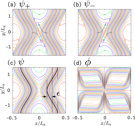
Figure 1: Contours of $\psi_{\pm}$, $\psi$ and $\phi$ when $\epsilon=5\rho_{s}$, where $\rho_{s}=d_{e}=0.02L_{x}$, $L_{y}/L_{x}=\pi$.

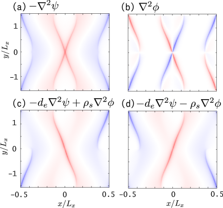
Figure 2: Intensity distributions (red: positive, blue: negative) of the current $-\nabla^{2}\psi$, vorticity $\nabla^{2}\phi$ and $-d_{e}\nabla^{2}\psi\pm\rho_{s}\nabla^{2}\phi$ when $\epsilon=5\rho_{s}$, where $\rho_{s}=d_{e}=0.02L_{x}$, $L_{y}/L_{x}=\pi$.

The nonlinear evolution of (1) and (2) was studied in earlier works Cafaro ; Grasso ; Grasso2 ; Bhattacharjee , and we reproduce the main features, as shown in Figs. 1 and 2. Since $\psi_{+}$ and $\psi_{-}$ are frozen-in variables, their contours preserve topology as seen in Figs. 1(a) and (b) (where the arrows depict the fluid motions generated by $\phi_{\pm}$). Then, spiky peeks of $\psi_{+}$ and $\psi_{-}$ are formed and their ridge lines look like the shapes of “$\backslash$” and “/”, respectively, around the origin. In light of the definition (6), the current and vorticity distributions can be directly calculated by using $\psi_{\pm}$ and shown in Figs. 2(a) and (b), which exhibit a “X”-shaped current-vortex layer Aydemir ; Cafaro whose width is of order $d_{e}=\rho_{s}$. We also note from Figs. 2(c) and (d) that a relation $d_{e}|\nabla^{2}\psi|\simeq\rho_{s}|\nabla^{2}\phi|$ holds inside the layer (except at the reconnection points).

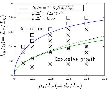
Figure 3: Parameters $k_{y}$ and $\rho_{s}(=d_{e})$ that result in explosive growth ($\times$ and $*$) and saturation ($\square$). The maximum linear growth rate occurs at points $*$ for each $\rho_{s}$.

As indicated in Fig. 1(c), we denote the maximum displacement of the field lines at $x=\pm L_{x}/4$ by $\epsilon$ and numerically measure it from the displacement of the contour $\psi=0$. We have run simulations with various combinations of $L_{x}/L_{y}$ and $\rho_{s}/L_{x}(=d_{e}/L_{x})$, and investigated whether $\epsilon$ grows explosively or not. Our results are summarized in Fig. 3, where it should be recalled that the tearing mode is linearly unstable at all points in this figure since $0<L_{x}/L_{y}<1$. The linear growth rate achieves its numerical maximum at points indicated by the asterisk ($*$) for each fixed $\rho_{s}$, which agrees with the theoretical prediction (12) [and also (14) for $k_{y}/\alpha<0.377$]. The square symbol ($\square$) indicates points where exponential growth $\epsilon\propto e^{\gamma t}$ (with the linear growth rate $\gamma$) stalls before $\epsilon$ reaches $\rho_{s}$. On the other hand, at the crosses ($\times$) and asterisks ($*$) the exponential growth is accelerated when $\epsilon$ gets larger than $\rho_{s}$. These two regimes seem to be divided by a curve $\rho_{s}\Delta^{\prime}\sim 0.65$.

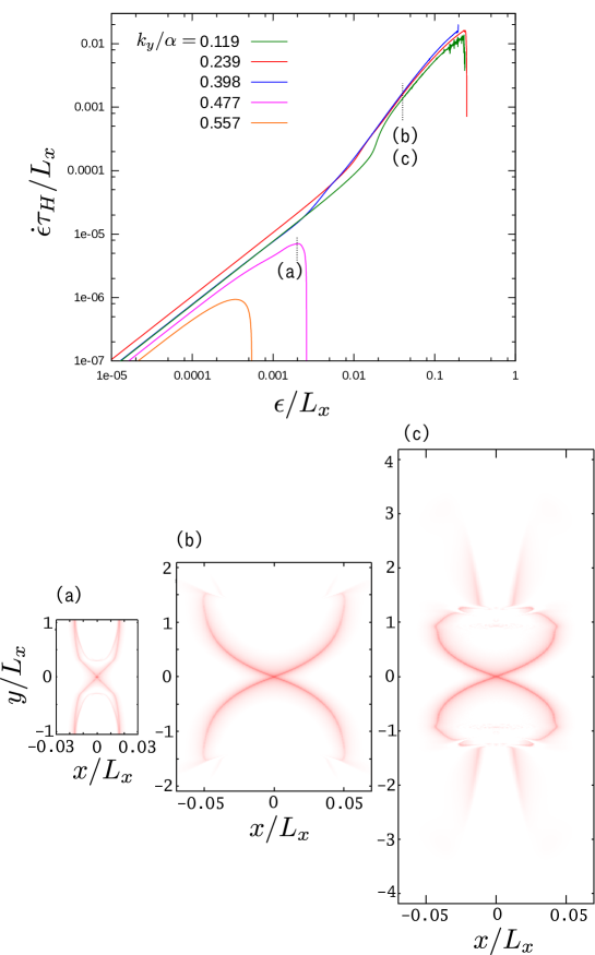
Figure 4: Logarithmic plots of the displacement $\epsilon$ versus its time-derivative $\dot{\epsilon}$, where $d_{e}=\rho_{s}=0.01$, and the current distributions (a) at $\epsilon=0.002L_{x}$ for $k_{y}/\alpha=0.477$, (b) at $\epsilon=0.04L_{x}$ for $k_{y}/\alpha=0.239$ and (c) at $\epsilon=0.04L_{x}$ for $k_{y}/\alpha=0.119$.

The above mentioned tendencies are demonstrated in Fig. 4, which is a logarithmic plot of $\dot{\epsilon}$ versus $\epsilon$ for the case $\rho_{s}/L_{x}=0.01$. For $k_{y}/\alpha=0.477$ and $0.557$, which belong to the saturation regime $\rho_{s}\Delta^{\prime}\lesssim 0.65$, the current-vortex layer spirals around the O-point as shown in Fig. 4(a) and the growth of $\epsilon$ decelerates. Although this occurs in an early nonlinear phase $\epsilon<\rho_{s}$ in our results, we note that the saturation mechanism is similar to the one found by Grasso et al. Grasso2 , namely, the phase mixing of the Lagrangian (or frozen-in) invariants $\psi_{\pm}$ leads to a new “macroscopic” stationary state. For the cases of $k_{y}/\alpha=0.119$, 0.239, and 0.398, which belong to $\rho_{s}\Delta^{\prime}\gtrsim 0.65$, we observe a transition from the exponential growth $\dot{\epsilon}\propto\epsilon$ to an explosive growth $\dot{\epsilon}\propto\epsilon^{n}$ ($n>1$) around $\epsilon\sim\rho_{s}$, and the latter continues until the reconnection completes at $\epsilon=L_{x}/4$. We further note that, for the small $k_{y}/\alpha=0.119$, a local X-shaped layer is generated spontaneously around the reconnection point and it expands faster than the global one that originates from the linear eigenmode [see Fig. 2(c)]. By comparing the case $k_{y}=0.119$ with $k_{y}=0.239$ at the same amplitude $\epsilon=0.04L_{x}$, we find that this local X-shaped structure around the origin in Fig. 2(c) is identical to that in Fig. 2(b). Therefore, the explosive reconnection seems to be attributed to the fast expansion of the local X-shape with a certain optimal size that is independent of the domain length $L_{y}=2\pi/k_{y}$. In fact, the nonlinear growth rates for $k_{y}=0.119$, 0.239, and $0.398$ are eventually comparable for $\epsilon\gtrsim 0.02$ because the released magnetic energies are almost the same regardless of $k_{y}$.

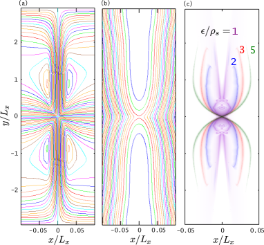
Figure 5: Contours of (a) $\phi$ and (b) $\psi$ at $\epsilon=0.015L_{x}=3\rho_{s}$ and (c) current distributions at $\epsilon/\rho_{s}=1,2,3,5$, where $d_{e}=\rho_{s}=0.005L_{x}$, $k_{y}/\alpha=k_{y,{\rm max}}/\alpha=0.171$.

We remark that the length of the local X-shape is not simply related to the wavelength $2\pi/k_{y,{\rm max}}$ of the most linearly unstable mode. For $d_{e}=\rho_{s}=0.005L_{x}$ and $k_{y}=k_{y,{\rm max}}=0.171\alpha$, Figs. 5(a) and (b) give a closer look at the contours of $\phi$ and $\psi$, respectively, at $\epsilon=3\rho_{s}$, and Fig. 5(c) shows the shapes of the current layer observed at $\epsilon/\rho_{s}=1,2,3$, and 5. As can be seen from Fig. 5(c), a local X-shape appears and expands quickly in the nonlinear phase $\epsilon>\rho_{s}$ even though this reconnection is triggered by the most linearly unstable tearing mode $k_{y}=k_{y,{\rm max}}$. Under the same conditions, the evolution of the energies $E_{V,T,B,C}$ defined by (3) is shown in Fig. 6 (where the total energy conservation $E=E_{0}=$ const. is satisfied numerically with sufficient accuracy). In the linear phase $\epsilon\ll\rho_{s}=0.005L_{x}$, the magnetic energy $E_{B}$ is transformed into $E_{V},E_{T}$ and $E_{C}$ at different but comparable rates. However, in the nonlinear phase $\epsilon>\rho_{s}$, we note that the magnetic energy is exclusively transformed into the ion flow energy $E_{V}$ and the energy balance $\delta E_{V}+\delta E_{B}\simeq 0$ is satisfied approximately. Since $\delta E_{T}$ and $\delta E_{C}$ are negligible, we infer that the nonlinear dynamics is dominantly governed by the ideal MHD equation ($d_{e},\rho_{s}\rightarrow 0$). This fact motivates us to regard $K:=E_{V}$ and $W:=E_{B}$ as the kinetic and potential energies, respectively, according to the MHD Lagrangian theory.

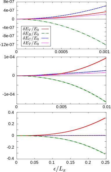
Figure 6: Changes of energies $E_{V},E_{B},E_{C}$ and $E_{T}$ versus $\epsilon$, where $d_{e}=\rho_{s}=0.005L_{x}$, $k_{y}/\alpha=k_{y,{\rm max}}/\alpha=0.171$.

IV Theoretical model

In this section, we develop a theoretical model to explain the explosive growth of $\epsilon$ in the nonlinear phase $d_{e}=\rho_{s}\ll\epsilon\ll L_{x}/4$. The current-vortex layers are obviously the boundary layers caused by the two-fluid effects and their width should be of order $d_{e}=\rho_{s}$. The ideal MHD equations, (1) and (2) with $d_{e}=\rho_{s}=0$, would be satisfied approximately outside the boundary layers. Moreover, we also assume that $\phi$ and $\psi$ are continuous across the boundary layers, because $E_{C}=\int d_{e}^{2}|\nabla^{2}\psi|^{2}d^{2}x/2$ and $E_{T}=\int\rho_{s}^{2}|\nabla^{2}\phi|^{2}d^{2}x/2$ are negligible in the energy conservation (Fig. 6) in the limit of $d_{e},\rho_{s}\rightarrow 0$. Note that $\nabla\psi$ and $\nabla\phi$ may be discontinuous across the layer because it is a current-vortex layer.

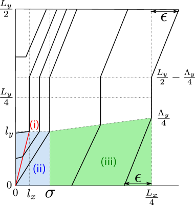
Figure 7: Local reconnection model.

Based on these assumptions, we consider a family of virtual displacements that generates a local X-shaped current-vortex layer, and then seek the displacement that decreases the magnetic (or potential) energy most effectively. Our reconnection model is illustrated in Fig. 7, where we show only the first quadrant around the origin owing to the parity (10). In Fig. 7, the magnetic field lines are assumed to be piecewise-linear and the red line denotes the boundary layer (i.e., the upper right part of the X-shape).

We will mainly focus on the three regions: (i) boundary layer (ii) inner solution with a X-shaped layer (iii) external solution. These regions are characterized by four parameters $\Lambda_{y},\sigma,l_{x},l_{y}$ as follows. First, the position of the boundary layer is specified by $(l_{x},l_{y})$. Second, the displacement of the field line that is about to reconnect at the origin is denoted by $\sigma$, which can be also regarded as the half width of the local island. Finally, to allow for local reconnection, we introduce the “wavelength” $\Lambda_{y}$ of the displacement at $x=L_{x}/4$, which may be smaller than the wavelength $L_{y}(=2\pi/k_{y})$ of the linear tearing mode. We will assume the following orderings among these parameters:

$$d_{e}=\rho_{s}\ll\epsilon\leq\sigma\ll L_{x}/4,\quad l_{x}<\sigma\ll l_{y}\leq\Lambda_{y}/4\leq L_{y}/4.$$ (16)

IV.1 Matching conditions across the boundary layer

First, we focus on a neighborhood of (i) the boundary layer and introduce a local coordinate system $(X,Y)$ in the frame moving with the boundary layer, so that the $X$ and $Y$ directions are respectively normal and tangent to the layer (see Fig. 8). Let the inner region of the boundary layer be $-\delta<X<\delta$, where $\delta\sim d_{e}=\rho_{s}$. In this coordinate system, the velocity $\bm{v}$ and the Alfvén velocity $\bm{b}=\bm{B}/\sqrt{\mu_{0}\rho_{0}}$ are assumed to be uniform outside the layer. Using the continuities of $\psi$ and $\phi$ across the layer, we assign linear functions,

$$\begin{cases}\psi=\psi_{c}-b_{t}^{(d)}X+b_{n}Y,\\ \phi=\phi_{c}+v_{t}^{(d)}X-v_{n}Y,\end{cases}$$ (17)

on the down-stream side ($X<-\delta$) and

$$\begin{cases}\psi=\psi_{c}-b_{t}^{(u)}X+b_{n}Y,\\ \phi=\phi_{c}+v_{t}^{(u)}X-v_{n}Y,\end{cases}$$ (18)

on the up-stream side ($X>\delta$), where all coefficients depend only on time. The discontinuities of the tangential components, $b_{t}^{(d)}\neq b_{t}^{(u)}$ and $v_{t}^{(d)}\neq v_{t}^{(u)}$, indicate the presence of a current-vortex layer within $[-\delta,\delta]$.

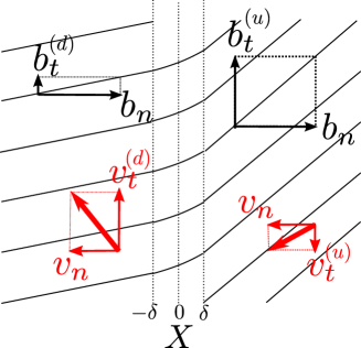
Figure 8: Neighborhood of the current-vortex layer.

Since we have assumed that $\partial_{t}\psi+[\phi,\psi]=0$ holds outside the layer, $[\phi,\psi]$ must be also continuous, namely,

$$v_{t}^{(d)}b_{n}-v_{n}b_{t}^{(d)}=v_{t}^{(u)}b_{n}-v_{n}b_{t}^{(u)},$$ (19)

is one of the matching conditions between (17) and (18).

Moreover, the conservation laws of $\psi_{\pm}$ require that $\psi_{-}$ has a spiky peek within the boundary layer whereas $\psi_{+}$ does not [see Figs. 1(a) and (b)]. Since $\psi_{+}\simeq\psi$ holds, we find a relation,

$$d_{e}\nabla^{2}\psi\simeq\rho_{s}\nabla^{2}\phi\quad\mbox{on}\quad[-\delta,\delta],$$ (20)

which specifies the ratio between a current peak ($-\nabla^{2}\psi$) and a vorticity peak ($\nabla^{2}\phi$) inside the layer. We have already noticed this relation in Fig. 2. By integrating these current and vorticity distributions over $[-\delta,\delta]$, we obtain another matching condition,

$$-\rho_{s}(v_{t}^{(u)}-v_{t}^{(d)})=d_{e}(b_{t}^{(u)}-b_{t}^{(d)}).$$ (21)

When the boundary layer is moving at a speed $V_{n}$ in the $X$ direction, the condition (19) is transformed to

$$v_{t}^{(d)}b_{n}-(v_{n}-V_{n})b_{t}^{(d)}=v_{t}^{(u)}b_{n}-(v_{n}-V_{n})b_{t}^{(u)},$$ (22)

in the rest frame, and the condition (21) is unchanged. Since these conditons also yield

$$\rho_{s}(v_{n}-V_{n})=-d_{e}b_{n},$$ (23)

we need to impose at least two matching conditions among (21), (22) and (23).

IV.2 Modeling of the X-shaped boundary layer

Next, we consider (ii) the inner solution that contains the X-shaped boundary layer. The detailed sketch of this region is given in Fig. 9, where the displacement map $(x_{0},y_{0})\mapsto(x,y)$ on the up-stream side (i.e., the right side of the boundary layer) is simply modeled by

$$x=x_{0}+\frac{\sigma}{l_{y}}(y_{0}-l_{y})\quad\mbox{ and }\quad y=y_{0}.$$ (24)

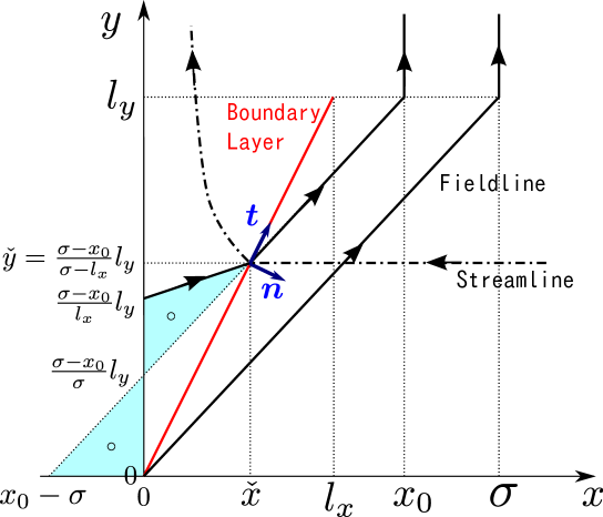
Figure 9: First quadrant of the X-shaped boundary layer.

This displacement map fully determines $\psi$ and $\phi$ on the up-stream side as follows. Since $\sigma\ll L_{x}/4$ is assumed in (16), we expand the equilibrium flux function,

$$\psi^{(0)}(x,y)=\psi_{0}\cos(\alpha x)=\psi_{0}\left(1-\frac{\alpha^{2}}{2}x^{2}\right)+O(x^{3}),$$ (25)

and neglect $O(x^{3})$ in this region $[0,\sigma]$. Except on the boundary layer, the magnetic flux $\psi$ is frozen into the displacement and hence becomes

$$\psi^{(u)}(x,y,t)=\psi^{(0)}(x_{0},y_{0})= \psi_{0}-\psi_{0}\frac{\alpha^{2}}{2}\left[x-\frac{\sigma}{l_{y}}(y-l_{y})\right]^{2},$$ (26)

on the up-stream side. By regarding the parameters $\sigma(t),l_{x}(t),l_{y}(t)$ as functions of time, the time derivative of the displacement map gives the stream function,

$$\phi^{(u)}(x,y,t)=-\dot{\mathsf{s}}_{y}\frac{y^{2}}{2}+\dot{\sigma}y,$$ (27)

where $\mathsf{s}_{y}=\sigma/l_{y}$, and the parity $\phi(x,0,t)=0$ has been used as the boundary condition.

Now, let us consider a magnetic field line that is labeled by its initial position $x=x_{0}$ (where $l_{x}<x_{0}<\sigma$). When this field line is displaced by the map, it intersects with the boundary layer at

$$(\check{x},\check{y})=\left(\frac{\sigma-x_{0}}{\sigma-l_{x}}l_{x},\frac{\sigma-x_{0}}{\sigma-l_{x}}l_{y}\right).$$ (28)

The tangent and normal unit vectors to the boundary layer are respectively given by $\bm{t}=(l_{x},l_{y})/|\bm{l}|$ and $\bm{n}=(l_{y},-l_{x})/|\bm{l}|$, where $|\bm{l}|=\sqrt{l_{x}^{2}+l_{y}^{2}}$. Therefore, the normal and tangent components at $(\check{x},\check{y})$ are calculated as follows;

$$b_{n}^{(u)}= \tau_{H}^{-1}(\sigma-l_{x})\frac{x_{0}}{|\bm{l}|}\quad(>0),$$ (29)

$$b_{t}^{(u)}= \tau_{H}^{-1}\left(\frac{l_{x}}{l_{y}}\sigma+l_{y}\right)\frac{x_{0}}{|\bm{l}|}\quad(>0),$$ (30)

$$v_{n}^{(u)}= \frac{l_{y}}{|\bm{l}|}(\dot{\mathsf{s}}_{y}\check{y}-\dot{\sigma})\quad(<0),$$ (31)

$$v_{t}^{(u)}= \frac{l_{x}}{|\bm{l}|}(\dot{\mathsf{s}}_{y}\check{y}-\dot{\sigma})\quad(<0),$$ (32)

where $\tau_{H}^{-1}:=\psi_{0}\alpha^{2}$.

Next, we consider the down-stream side, on which the magnetic field lines are again approximated by straight lines as shown in Fig. 9. Since the displacement map is area-preserving, the same field line that passes through $(\check{x},\check{y})$ is found to be

$$y=\frac{l_{y}}{l_{x}}\left(\frac{2l_{x}-\sigma}{l_{x}}x+\sigma-x_{0}\right),$$ (33)

by equating the areas of the two blue triangles in Fig. 9. Using the fact that the value of $\psi$ is again $\psi^{(0)}(x_{0},y_{0})$ on this field line, a straightforward calculation results in

$$\psi^{(d)}(x,y,t)= \tau_{H}^{-1}\frac{l_{x}}{l_{y}}\left(\sigma y-\frac{l_{x}}{l_{y}}\frac{y^{2}}{2}+\frac{2l_{x}-\sigma}{l_{x}}xy\right)$$

$$+\tau_{H}^{-1}\frac{2l_{x}-\sigma}{l_{x}}\left(-\sigma x-\frac{2l_{x}-\sigma}{l_{x}}\frac{x^{2}}{2}\right)+\psi_{0}-\tau_{H}^{-1}\frac{\sigma^{2}}{2}.$$ (34)

The field line (33) also moves in time because of the time dependence of $l_{x},l_{y}$ and $\sigma$. By imposing the boundary condition $\phi(0,y,t)=0$ on the $y$ axis, the associated incompressible flow can be determined uniquely as

$$\phi^{(d)}(x,y) =-\frac{\dot{\mathsf{s}}_{y}-2\dot{\beta}}{\beta}\frac{x^{2}}{2}-\frac{\dot{\beta}}{\beta}xy+\frac{\dot{\sigma}}{\beta}x,$$ (35)

where $\beta=l_{x}/l_{y}$. We thus obtain, at $(\check{x},\check{y})$,

$$b_{t}^{(d)}= \tau_{H}^{-1}\left(\frac{l_{x}^{2}}{l_{y}}+\frac{2l_{x}-\sigma}{l_{x}}l_{y}\right)\frac{x_{0}}{|\bm{l}|},$$ (36)

$$v_{t}^{(d)}= \frac{l_{x}}{|\bm{l}|}\left[\left(\frac{|\bm{l}|^{2}}{l_{x}^{2}}\dot{\beta}-\frac{l_{y}^{2}}{l_{x}^{2}}\dot{\mathsf{s}}_{y}\right)\check{y}+\frac{l_{y}^{2}}{l_{x}^{2}}\dot{\sigma}\right],$$ (37)

and confirm that $b_{n}^{(d)}=b_{n}^{(u)}$ and $v_{n}^{(d)}=v_{n}^{(u)}$ are indeed satisfied.

The speed $V_{n}$ for movement of the boundary layer at $(\check{x},\check{y})$ is calculated by using the angle $\theta$ between the boundary layer and the $y$ axis ($\tan\theta=l_{x}/l_{y}$),

$$V_{n}=\sqrt{\check{x}^{2}+\check{y}^{2}}\dot{\theta}=\frac{l_{y}}{|\bm{l}|}\dot{\beta}\check{y}.$$ (38)

Now, we are ready to impose the matching conditions on these up- and down-stream solutions. It is interesting to note that the matching condition (22) is already satisfied because we have taken the continuities of $\psi$ and $\phi$ into account in the above construction. The matching condition (21) at $(\check{x},\check{y})$ gives

$$\dot{\zeta}\frac{\sigma-x_{0}}{\zeta}-\dot{\sigma}=-\tau_{H}^{-1}x_{0}\zeta,$$ (39)

where $\zeta:=\mathsf{s}_{y}-\beta=(\sigma-l_{x})/l_{y}$. This condition must be satisfied for all points $(\check{x},\check{y})$ on the boundary layer (that is, for all $x_{0}\in[l_{x},\sigma]$), which requires both $\dot{\zeta}\sigma=\dot{\sigma}\zeta$ and $\dot{\zeta}=\tau_{H}^{-1}\zeta^{2}$ to be satisfied. The former gives a constant of motion,

$$\frac{\sigma}{\zeta}=\frac{\sigma}{\sigma-l_{x}}l_{y}=l_{y0}=\mbox{const.},$$ (40)

and the latter gives an evolution equation,

$$\dot{\sigma}=\frac{1}{l_{y0}\tau_{H}}\sigma^{2}.$$ (41)

Although the constant $l_{y0}(>0)$ is still unknown unless $l_{x}$ and $l_{y}$ are specified, the displacement $\sigma$ turns out to grow explosively due to the presence of the X-shaped boundary layer. These parameters $l_{x}$, $l_{y}$ and $l_{y0}$ will be determined later when this inner solution is matched with the external solution and the global energy balance is taken into account.

IV.3 External solution

Now consider (iii), the external solution of Fig. 7. Even though we discuss the nonlinear phase, the displacement $\sigma$ (or the island half-width) must be small $\sigma\ll L_{x}/4$ as well as the growth rate $\dot{\sigma}/\sigma\ll\tau_{H}^{-1}$ in comparison with the equilibrium space-time scale. Therefore, we expect the external solution to be similar to the well-known eigenfunction of the linear tearing mode. This treatment for the external solution is commonly used in Rutherford’s theory Rutherford ; White , while we introduce the arbitrary wavelength $\Lambda_{y}(<L_{y})$ of the linear tearing mode in this work. Namely, the displacement in the $x$ direction is given by $\xi(x,y)=\epsilon\hat{\xi}(x)\cos(2\pi y/\Lambda_{y})$ for $y\in[0,\Lambda_{y}/4]$ where the eigenfunction,

$$\hat{\xi}(x)=-\frac{\cos\left[\sqrt{1-(L_{x}/\Lambda_{y})^{2}}\left(\alpha|x|-\frac{\pi}{2}\right)\right]}{\sin\alpha x},$$ (42)

is normalized so as to satisfy $\hat{\xi}(L_{x}/4)=-1$ and $\hat{\xi}(-L_{x}/4)=1$. Taylor expansion of $\hat{\xi}$ around $x=0$ on the positive side ($x>0$) gives

$$\hat{\xi}(x)= -\left(\frac{2}{\tilde{\Delta}^{\prime}x}+1\right)\sqrt{1-(L_{x}/\Lambda_{y})^{2}}\cos\left[\sqrt{1-(L_{x}/\Lambda_{y})^{2}}\frac{\pi}{2}\right]+O(x),$$ (43)

where the tearing index $\tilde{\Delta}^{\prime}$ for the wavelength $\Lambda_{y}$ is

$$\tilde{\Delta}^{\prime}=2\alpha\sqrt{1-(L_{x}/\Lambda_{y})^{2}}\tan\left[\sqrt{1-(L_{x}/\Lambda_{y})^{2}}\frac{\pi}{2}\right].$$ (44)

Since the dependence of $\hat{\xi}$ on $\Lambda_{y}$ is complicated, we again restrict the range of $\tilde{\Delta}^{\prime}$ to the large $\Delta^{\prime}$ regime,

$$\tilde{\Delta}^{\prime}>\Delta^{\prime}_{c}:=100/L_{x}\quad(\mbox{or }\Lambda_{y}/L_{x}>2.5),$$ (45)

as we have done in the linear theory. Then, we can use the following approximations:

$$\hat{\xi}(x) \simeq-1-\frac{2}{\tilde{\Delta}^{\prime}x}+O(x),$$ (46)

$$\tilde{\Delta}^{\prime} \simeq 16\frac{\Lambda_{y}^{2}}{L_{x}^{3}}.$$ (47)

The critical value $\Delta^{\prime}_{c}=100/L_{x}$ is, of course, specific to the equilibrium state (8).

This external solution is matched to the inner solution by

$$-\sigma=\epsilon\hat{\xi}(\sigma)=-\epsilon\left(1+\frac{2}{\tilde{\Delta}^{\prime}\sigma}\right)+O(\epsilon\sigma),$$ (48)

which gives, by neglecting $O(\epsilon\sigma)$,

$$\sigma= \epsilon\frac{1+\sqrt{1+\frac{8}{\epsilon\tilde{\Delta}^{\prime}}}}{2}.$$ (49)

Note that $\sigma$ is larger than $\epsilon$ as illustrated in Fig. 7. Since the displacement map is area-preserving, we determine $l_{y}$ by the relation,

$$\sigma l_{y}=\epsilon\frac{\Lambda_{y}}{4}.$$ (50)

IV.4 Energy balance

In linear tearing mode theory, the released magnetic energy via reconnection is estimated by

$$\delta W= -\epsilon^{2}\frac{L_{y}}{2}\left.\hat{\psi}\frac{d\hat{\psi}}{dx}\right|_{x=-a}^{x=a},$$ (51)

in terms of the perturbed flux function $\hat{\psi}=-(d\psi^{(0)}/dx)\hat{\xi}=\tau_{H}^{-1}x\hat{\xi}$, where $2a(\ll L_{x})$ is the width of the boundary layer at $x=0$ (see Appendix A of Ref. Hirota ). This is true if the eigenfunction $\hat{\psi}(x)$ is smoothed out and flattened within the layer $[-a,a]$ by some sort of nonideal MHD effects.

For the nonlinear phase in question, we simply replace $a$ by $\sigma$ (and $L_{y}$ by $\Lambda_{y}$) because the flux function $\psi$ is flattened within $[-\sigma,\sigma]$ by the formation of a magnetic island. This idea is similar to the finite-amplitude generalization of $\Delta^{\prime}$ which is made by White et al. White for the purpose of introducing a saturation phase to Rutherford’s theory. In either case, the island width $2\sigma$ grows as far as $\hat{\psi}d\hat{\psi}/dx|_{x=-\sigma}^{x=+\sigma}>0$. Using the Taylor expansion (46) and the relation (50), we obtain

$$\delta W=-\epsilon^{2}\frac{\Lambda_{y}}{2}\hat{\psi}\frac{d\hat{\psi}}{dx}\big{|}_{x=-\sigma}^{x=\sigma}=-4l_{y}\tau_{H}^{-2}\sigma^{3}.$$ (52)

We remark that the magnetic energy in the area $[0,\sigma]\times[0,l_{y}]$ at the equilibrium state ($t=0$) is also of the order of $l_{y}\tau_{H}^{-2}\sigma^{3}$. Since this area is mapped to the internal region of the magnetic island after the displacement, we can expect a corresponding decrease in the total magnetic energy, which agrees with the estimation (52).

In order to satisfy the energy conservation $\delta K+\delta W=0$, the kinetic energy is required to satisfy $\delta K\propto l_{y}\sigma^{3}$. To be concise, let us assume $l_{y}=$ const. a priori because this assumption turns out to yield the desired scaling $\delta K\propto\sigma^{3}$ as follows.

Since the kinetic energy is mostly concentrated on the down-stream side due to the outflow from the X-shaped vortex layer, we use $\phi^{(d)}$ in (35) and the orderings $l_{y}\gg l_{x}$ and $l_{y}\gg\sigma$ to estimate the kinetic energy in the down-stream region as

$$\int_{0}^{l_{y}}dy\int_{0}^{\frac{l_{x}}{l_{y}}y}dx\frac{|\nabla\phi|^{2}}{2}= \left(1+\frac{l_{x}^{2}}{6\sigma^{2}}\right)\frac{\dot{\sigma}^{2}}{2}\frac{l_{y}^{3}}{2l_{x}}[1+O(l_{x}/l_{y})+O(\sigma/l_{y})]$$

$$\simeq \frac{\dot{\sigma}^{2}}{2}\frac{l_{y}^{3}}{2l_{x}},$$ (53)

where we have neglected $l_{x}^{2}/6\sigma^{2}$ in the last expression since $l_{x}/\sigma=1-l_{y}/l_{y0}$ is now constant and less than unity. The same estimate is more easily obtained as follows. Consider the flow passing through the box $[0,l_{x}]\times[0,l_{y}]$. Since the inflow velocity into the box is at most $\dot{\sigma}$, the outflow velocity, say $\overline{v}_{y}$, is roughly determined by the incompressibility condition,

$$\dot{\sigma}l_{y}=\bar{v}_{y}l_{x},$$ (54)

where $\bar{v}_{y}\gg\dot{\sigma}$ owing to $l_{y}\gg l_{x}$. The kinetic energy density $\bar{v}_{y}^{2}/2$ multiplied by the area $l_{x}l_{y}/2$ reproduces the same estimate as (53).

In fact, the outflow also exists over the area $[0,l_{x}]\times[l_{y},L_{y}/2]$ in Fig. 7 and there are eight equivalent areas in the whole domain according to the parity. Therefore, a plausible estimate of the total kinetic energy is

$$\delta K=8\frac{\bar{v}_{y}^{2}}{2}\left[\frac{l_{x}l_{y}}{2}+l_{x}\left(\frac{L_{y}}{2}-l_{y}\right)\right]=2\frac{\dot{\sigma}^{2}l_{y}^{2}}{l_{x}}\left(L_{y}-l_{y}\right)=2\frac{\sigma^{3}l_{y}^{2}}{l_{y0}^{2}\tau_{H}^{2}}\frac{L_{y}-l_{y}}{1-l_{y}/l_{y0}},$$ (55)

where the evolution equation (41) for $\sigma$ has been used. Since this $\delta K$ is proportional to $\sigma^{3}$, we can impose the energy conservation law $\delta K+\delta W=0$, which determines $l_{y0}$ with respect to $l_{y}$,

$$\frac{l_{y0}}{l_{y}}=\frac{1+\sqrt{2\frac{L_{y}}{l_{y}}-1}}{2}.$$ (56)

Given this $l_{y0}$, the rate of decrease in the magnetic energy

$$\frac{\partial_{t}(\delta W)}{\delta W}=\frac{3\sigma}{l_{y0}\tau_{H}}$$ (57)

indicates that the shorter the length $l_{y}$, the faster the magnetic energy decreases. Thus, the local reconnection (i.e., the local X-shape) develops faster than the global one.

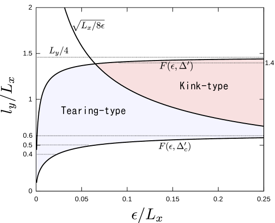
Figure 10: Range of $l_{y}$ corresponding to $\Delta_{c}^{\prime}<\tilde{\Delta}^{\prime}\leq\Delta^{\prime}$ for the case of $k_{y}/\alpha=L_{x}/L_{y}=0.171$.

However, there is a lower bound for $l_{y}$ since this argument is based on the assumption $\Delta_{c}^{\prime}<\tilde{\Delta}^{\prime}\leq\Delta^{\prime}$, for which the approximation $\tilde{\Delta}^{\prime}=16\Lambda_{y}^{2}/L_{x}^{3}$ (and $\Delta^{\prime}=16L_{y}^{2}/L_{x}^{3}$) is valid. Using (49) and (50) with this approximation, $l_{y}$ can be regarded as a function of $\epsilon$ and $\tilde{\Delta}^{\prime}$,

$$\frac{l_{y}}{L_{x}}=\frac{1}{8}\frac{\sqrt{L_{x}\tilde{\Delta}^{\prime}}}{1+\sqrt{1+\frac{8}{\epsilon\tilde{\Delta}^{\prime}}}}=:F(\epsilon,\tilde{\Delta}^{\prime}),$$ (58)

and hence $l_{y}/L_{x}$ should lie between $F(\epsilon,\Delta^{\prime}_{c})$ and $F(\epsilon,\Delta^{\prime})$ as shown in Fig. 10.

IV.5 Scaling of the explosive growth

By rewriting (58) as

$$\left(1+\sqrt{1+\frac{8}{\epsilon\tilde{\Delta}^{\prime}}}\right)\sqrt{\frac{8}{\epsilon\tilde{\Delta}^{\prime}}}=\frac{L_{x}}{l_{y}}\sqrt{\frac{L_{x}}{8\epsilon}},$$ (59)

this relation is found to have two kinds of scaling depending on whether its right hand side is much smaller or larger than unity,

First, when $l_{y}/L_{x}\gg\sqrt{L_{x}/8\epsilon}$, the relation reduces to

$$\frac{8}{\epsilon\tilde{\Delta}^{\prime}}=\frac{L_{x}^{3}}{32l_{y}^{2}\epsilon}\ll 1.$$ (60)

Since $\sigma\simeq\epsilon$ in this case, we obtain the same explosive growth as (41),

$$\dot{\epsilon}=\frac{\epsilon^{2}}{\tau_{H}l_{y0}},$$ (61)

in terms of the displacement $\epsilon$ at $x=L_{x}/4$. We refer this scaling as kink-type because $\tilde{\Delta}^{\prime}$ is so large that the external solution is similar to the kink mode ($\sigma\simeq\epsilon$, $l_{y}\simeq\Lambda_{y}/4$).

On the other hand, when $l_{y}/L_{x}\ll\sqrt{L_{x}/8\epsilon}$, the relation (59) reduces to

$$\frac{8}{\epsilon\tilde{\Delta}^{\prime}}=\sqrt{\frac{L_{x}^{3}}{8l_{y}^{2}\epsilon}}\gg 1.$$ (62)

By noting that

$$\sigma\simeq\frac{\epsilon}{2}\sqrt{\frac{8}{\epsilon\tilde{\Delta}^{\prime}}}=\frac{\epsilon^{3/4}}{2}\left(\frac{L_{x}^{3}}{8l_{y}^{2}}\right)^{1/4},$$ (63)

the explosive growth (41) becomes

$$\dot{\epsilon}=\frac{\epsilon^{7/4}}{\tau_{H}l_{y0}}\frac{2}{3}\left(\frac{L_{x}^{3}}{8l_{y}^{2}}\right)^{1/4}.$$ (64)

We refer this scaling as tearing-type because $\tilde{\Delta}^{\prime}$ is so small that the external solution is similar to the tearing mode ($\sigma>\epsilon$, $l_{y}<\Lambda_{y}/4$).

The boundary line $l_{y}/L_{x}=\sqrt{L_{x}/8\epsilon}$ between the kink-type and tearing-type regimes is also drawn in Fig. 10. Since the magnetic energy is released more effectively for the smaller $l_{y}$, the fastest reconnection occurs near the lower bound $l_{y}/L_{x}=0.4\sim 0.6$. Figure 11 shows that the tearing-type scaling (64) for $l_{y}/L_{x}=0.4,0.5$, and $0.6$ agrees well with the simulation results. For comparison, we also draw the kink-type scaling (61) with $l_{y}=1.4L_{x}\simeq L_{y}/4$ as a global reconnection model, which is indeed slower than the simulation results. We can confirm that the stream lines in Fig. 5(a) are more like the tearing-type ($\sigma>\epsilon$, $l_{y}<\Lambda_{y}/4$). Although the current layers in Fig. 5(c) are actually curved, they are locally regarded as straight lines around the origin as in Fig. 7 and seem to have the length $l_{y}/L_{x}\simeq 0.5$. Note that the same $l_{y}/L_{x}\simeq 0.5$ is also observed in Fig. 4(b) and (c) since this $l_{y}/L_{x}$ is determined independently of $L_{y}$ and $d_{e}=\rho_{s}$ as shown in (58).

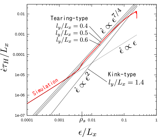
Figure 11: Logarithmic plot of the displacement $\epsilon$ versus its time-derivative $\dot{\epsilon}$ for $d_{e}=\rho_{s}=0.005L_{x}$, $k_{y}/\alpha=0.171$. Dotted lines are theoretically derived from the kink-type scaling (61) with $l_{y}/L_{x}=1.4$ and the tearing-type scaling (64) with $l_{y}/L_{x}=0.4,0.5,0.6$.

V Summary

We have investigated the nonlinear evolution of a collisionless tearing mode that can grow explosively with the formation of an X-shaped current-vortex layer due to the coexistence of electron inertia and temperature effects, where we have assumed $d_{e}=\rho_{s}$ for simplicity.

For the equilibrium state given in (8) and the wavenumber $k_{y}=2\pi/L_{y}$, the tearing mode is linearly unstable when the tearing index $\Delta^{\prime}$ (which is a function of $L_{y}/L_{x}$) is positive. The simulation results show that explosive growth occurs when $\Delta^{\prime}\gtrsim 0.65/\rho_{s}$. More specifically, the amplitude $\epsilon$ of the displacement at $x=\pm L_{x}/4$ exceeds $\rho_{s}$ and then grows explosively; $\dot{\epsilon}\propto\epsilon^{n}$, $n>1$. By observing this explosive phase in detail for $d_{e}=\rho_{s}<0.01$, we find that the X-shaped layer widens locally around the reconnection point and its length scale ($\simeq 2l_{y}$) seems to be unrelated to the wavelength $L_{y}$ (and $\Delta^{\prime}$ as well) of the linear eigenmode.

To explain this locally enhanced reconnection, we have developed a theoretical model in which the magnetic flux $\psi$ is assumed to be conserved (like ideal MHD) except within the thin X-shaped layer. Namely, the two-fluid conservation laws (4), (5) are invoked only within the layer to obtain the matching conditions across it. The external solution is approximated by a linear tearing eigenmode that has a shorter wavenumber $\Lambda_{y}$ than $L_{y}$ and a smaller tearing index $\tilde{\Delta}^{\prime}$ than $\Delta^{\prime}$. We have restricted our consideration to the range $\Delta_{c}^{\prime}(=100/L_{x})<\tilde{\Delta}^{\prime}\leq\Delta^{\prime}$ (or $2.5L_{x}<\Lambda_{y}<L_{y}$), in which a simple expression $\tilde{\Delta}^{\prime}=16\Lambda_{y}^{2}/L_{x}^{3}$ holds and the length of the local X-shape ($\simeq 2l_{y}$) is related to $\tilde{\Delta}^{\prime}$ by (58). As shown in Fig. 10, we have found that there are two kinds of scaling depending on whether the external solution is kink-type or tearing-type. The faster reconnection is theoretically predicted at the shorter $l_{y}$, namely, at the lower bound of this range, $l_{y}\simeq 0.5L_{x}$, $\tilde{\Delta}^{\prime}\simeq\Delta_{c}^{\prime}$ and $\Lambda_{y}\simeq 2.5L_{x}$, which belongs to the tearing-type regime. The simulation results indeed agree with the tearing-type scaling with the explosive growth rate $\dot{\epsilon}\propto\epsilon^{7/4}$ and they corroborate other properties predicted by this local reconnection model.

In comparison with the classical Petschek reconnection model Petschek in which the X-shaped boundary layer is composed of stationary slow-mode shocks, our model suggests that the X-shaped current-vortex layer is kinematically generated by ideal, incompressible and accelerated fluid motion in accordance with the two-fluid conservation laws and the energy conservation. The explosive growth rate (64) with $l_{y}\simeq 0.5L_{x}$ is moreover independent of the microscopic scale $d_{e}=\rho_{s}$ and hence reaches the Alfvén speed $\dot{\epsilon}\sim L_{x}^{2}/(\tau_{H}l_{y0})$ at the fully reconnected stage $\epsilon\sim L_{x}/4$. This is faster than the explosive growth $\dot{\epsilon}\sim k_{y}d_{e}^{1/2}\epsilon^{3/2}/\tau_{H}$ that is caused by the Y-shaped layer in the presence of only electron inertia (see our previous work Hirota ).

The two-field equations (1) and (2) can be derived from gyrokinetic and gyro-fluid equations by taking the fluid moments and then neglecting the ion pressure and electron and ion gyroradii Ishizawa ; Comisso . This fact suggests our present results are a barebones model for fast reconnection, but further generalizations including the case $d_{e}\neq\rho_{s}$ are suggested for future work. The existence of more than one microscopic scale gives rise to nested boundary layers, as already known from the linear analysis. The nonlinear evolution of such nested boundary layers would be more complicated than that of the single boundary layer ($d_{e}=\rho_{s}$) we have discussed. Nevertheless, if the outermost layer is sufficiently thinner than the island width and the energy balance is dominated by ideal MHD, we expect a similar X-shaped layer and explosive growth, since it is unlikely that any other structure can exist that is more efficient for releasing magnetic energy. Unfortunately, present computational resources are not enough to observe the explosive phase for a sufficiently long period in the presence of the nested bounded layers. For example, when $d_{e}\ll\rho_{s}$, linear analysis indicates that the innermost layer width $\sim d_{e}^{4/3}\rho_{s}^{-1/3}$ is even narrower than $d_{e}$ and demands more computational grids. Further advancements in computational performance and technique will be essential for studies of explosive reconnections in more general collisionless plasma models.

- (1) P.A. Sweet, Electromagnetic Phenomena in Cosmical Physics, IAU Symp. No. 6, edited by B. Lehnert (Cambridge Press, London, 1958). P. 123; E.N. Parker, J. Geophys. Res. 62, 509 (1957).
- (2) H.E. Petschek, Physics of Solar Flares. Edited by W. N. Hess (NASA SP-50, Washington DC, 1964), p. 425.
- (3) M. Ugai and T. Tsuda, J. Plasma Phys. 17, 337 (1977).
- (4) R.D. Hazeltine, M. Kotschenreuther and P. J. Morrison, Phys. Fluids 28, 2466 (1985).
- (5) T. J. Schep, F. Pegoraro and B. N. Kuvshinov, Phys. Plasmas, 1, 2843 (1994).
- (6) B. N. Kuvshinov, F. Pegoraro and T. J. Schep, Phys. Lett. A, 191, 296 (1994).
- (7) R. Fitzpatrick and F. Porcelli, Phys. Plasmas, 11 4713 (2004).
- (8) P. B. Snyder and G. W. Hammett, Phys. Plasmas, 8, 3199 (2001).
- (9) F. L. Waelbroeck and E. Tassi, Commun. Nonlinear Sci. Numer. Simul. 17, 2171 (2012).
- (10) E. A. Frieman and L. Chen, Phys. Fluids, 25, 502 (1982).
- (11) A. Zocco and A. A. Schekochihin, Phys. Plasmas 18 102309 (2011).
- (12) A. Y. Aydemir, Phys. Fluids B, 4, 2469 (1992).
- (13) M. Ottaviani and F. Porcelli, Phys. Rev. Lett., 71, 3802 (1993).
- (14) E. Cafaro, D. Grasso, F. Pegoraro, F. Porcelli and A. Saluzzi, Phys. Rev. Lett., 80, 4430 (1998).
- (15) A. Bhattacharjee, K. Germaschewski and C. S. Ng Phys. Plasmas, 12, 042305 (2005).
- (16) T. Matsumoto, H. Naitou, S. Tokuda and Y. Kishimoto, Phys. Plasmas 12, 092505 (2005)
- (17) A. Biancalani and B. D. Scott, Europhys. Lett. 97, 15005 (2012).
- (18) L. Comisso, D. Grasso, F. L. Waelbroeck and D. Borgogno, Phys. Plasmas 20, 092118 (2013).
- (19) A. Ishizawa and T.-H. Watanabe, Phys. Plasmas 20, 102116 (2013).
- (20) J. F. Drake, Phys. Fluids, 21, 1777 (1978).
- (21) B. Basu and B. Coppi, Phys. Fluids, 24, 465 (1981).
- (22) F. Porcelli, Phys. Rev. Lett., 66, 425 (1991).
- (23) P. H. Rutherford Phys. Fluids, 16, 1903 (1973).
- (24) R. B. White, D. A. Monticello, M. N. Rosenbluth and B. V. Waddell, Phys. Fluids, 20, 800 (1977).
- (25) M. Hirota, P.J. Morrison, Y. Ishii, M. Yagi and N. Aiba, Nucl. Fusion, 53, 063024 (2013).
- (26) R. D. Hazeltine, C. T. Hsu and P. J. Morrison, Phys. Fluids 30, 3204 (1987).
- (27) Morrison P.J. and J. M. Greene 1980 Phys. Rev. Letts. 45 790
- (28) Morrison P.J. 1998 Rev. Mod. Phys. 70 467
- (29) B. N. Kuvshinov, V. P. Lakhin, F. Pegoraro and T. J. Schep, J. Plasma Physics, 59, 727 (1998)
- (30) D. Grasso, F. Califano, F. Pegoraro and F. Porcelli, Plasma Phys. Control. Fusion, 41, 1497 (1999).
- (31) E. Tassi, P. J. Morrison, D. Grasso and F. Pegoraro Nucl. Fusion, 50, 034007 (2010).
- (32) D. Grasso, F. Califano, F. Pegoraro and F. Porcelli, Phys. Rev. Lett. 86, 5051 (2001).
- (33) D. Biskamp, Magnetic Reconnection in Plasmas (Cambridge University Press, Cambridge, 2000)