Quantum tight-binding chains with dissipative coupling

Abstract

We present a one-dimensional tight-binding chain of two-level systems coupled only through common dissipative Markovian reservoirs. This quantum chain can demonstrate anomalous thermodynamic behavior contradicting Fourier law. Population dynamics of individual systems of the chain is polynomial with the order determined by the initial state of the chain. The chain can simulate classically hard problems, such as multi-dimensional random walks.

1 Introduction

Coherent chains of interacting quantum systems represent a wide class of physical objects that define the behavior of matter under different physical conditions. Study of theoretical models for these objects, which was started by the epoch-making works by Hubbard [1] and Ising [2], covers both new forms of matter and new types of interactions [3]. One can coherently chain cooled atoms in optical lattices [3], Josephson qubits in microwave transmission lines [4], semiconductor quantum dots, etc. Interactions between systems can be of quite different physical nature: spin-exchange interactions or pseudospin interactions corresponding to the dipole optical transitions [5], tunneling [6], dipole-dipole interactions [7, 8], photonic interactions (Jaynes-Cummings-Hubbard model [9]) and many others. Recent applications of these models led to a number of new fundamental results. For example, 1D - chain of tunnel-coupled systems with two ends connected to heat reservoirs served as a model to justify the Fourier heat conduction law from the first principles and to provide microscopic definition of temperature [11, 12]. Other results to be mentioned are the directivity of collective spontaneous emission [7, 13]), possibility to transfer quantum states [16], the spatial propagation of Rabi oscillations (Rabi-waves) [14, 15], and quantum optical nonreciprocity of the medium in timed Dicke state [17].

It is of particular importance to study new types of interactions that determine the coherent behavior of coupled systems. Here we suggest to couple them in a chain by connecting them pair-wisely to common dissipative reservoirs. It is already well-known that coupling several quantum systems to the same dissipative reservoir allows to obtain a number of highly non-trivial effects. First of all, such a coupling can create a decoherence-free subspace [18, 19]. An arbitrary initial state is eventually transferred into this subspace. Thus, it is possible to produce non-classical and entangled states via dissipative dynamics even without any direct interaction between quantum systems [20]. This effect has many potential applications. For example, it was recently used in practice to protect the highly-entangled initial polarization states of photons from dephasing in optical fibers [21]. Moreover, combining coupling to the same reservoir with the nonlinear interaction between quantum systems, it is possible to produce nonlinear loss generating robustly a wide variety of non-classical states [22, 23, 24]. By adding external driving, a generated non-classical state can be preserved in the presence of an arbitrarily large linear loss [25].

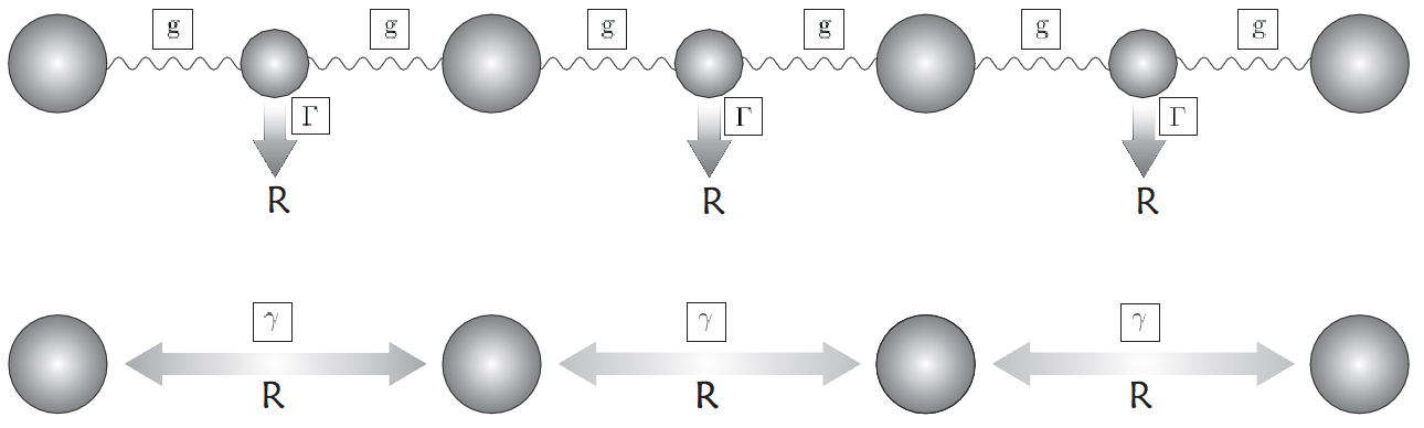
Figure 1: (above) A scheme of bipartite tight-binding spin-chain with some elements subjected to strong loss. This scheme is described by Eq. (11). (below) A scheme of dissipatively coupled tight-binding spin chain described by Eq. (1).

Here we show that by coupling a set of quantum systems through common Markovian reservoirs and forming one-dimensional tight-binding chain, it is possible to produce highly non-trivial dynamics. Such a dissipatively coupled set of just a few two-level system renders a possibility to reproduce dynamics of far more complex systems, such as classical heat reservoirs and multidimensional random networks. This dynamics can be "tuned" by choice of the initial state of the system.

We demonstrate that even for a few systems in the chain certain groups of matrix elements of the chain density matrix evolve according to equations formally coinciding with the equations describing classical random walks. For no more than one initial excitation in the chain, matrix elements of the single-excitation subspace evolve according to the equation describing two-dimensional classical random walk. Simultaneously, matrix elements describing coherences between the single-excitation and zero-excitation subspaces evolve according to the equation describing one-dimensional random walk. Taking more than one initial excitation in the chain, one is able to obtain dynamics governed by equations describing multi-dimensional classical random walks. This fact leads to a number of quite-counterintuitive consequences. Notwithstanding the Markovianity of reservoirs, a decay of excitation in any system of the chain is polynomial with the same power. By choosing the initial states, it is possible to obtain a population decay law $1/t^{2m+1}$, for an arbitrary $m>0$, provided that the chain is long enough. The sum of density matrix elements described by the random walk equation is conserved. So, one can observe rather peculiar thermodynamics-like behaviour of the chain. Despite seemingly classical character, this "thermodynamics" is quite anomalous. The stationary state of the chain can be entangled. Moreover, energy flow through the chain is not described by the Fourier law, whereas the flow of coherences is governed by it.

The outline of paper is as follows. In the Section 2 we introduce the concept of tight-binding dissipatively coupled quantum chain. Also, we show how this "quantum gadget" can be built in practice from usual tight-binding unitary chain by selectively applying strong dissipation to certain systems in the chain. In the Section 3 we derive equations for the simplest case of the chain dynamics corresponding to an initial state with no more than just one excitation. Already in this case the chain exhibits a rich variety of highly unusual phenomena. We highlight the thermodynamical analogies in the Section 4. In the Section 5 we analyze in more details possibilities of having different polynomial decay for specific choices of initial states of the chain. Then, in the Section 6 we discuss the dynamics of the chain in the case of multiple initial excitations demonstrating how conservation of coherences might arise in this case, too.

2 The chain

Here we are discussing dynamics of a set of quantum objects coupled only through common dissipative reservoirs. We are interested in dynamics arising for the case when our set is rather large (with the number of objects, $N\gg 1$). In this paper we consider one of the simplest cases of such a set, namely, a tight-binding one-dimensional chain of identical two-level systems (TLS), e. g., spins or pseudo-spins. The general scheme of such an arrangement is as follows. Each spin is supposed to be coupled to common Markovian reservoirs with one of two neighbors: $j$th TLS and $(j+1)$th TLS are coupled to common $j$th reservoir, $(j-1)$th TLS and $j$th TLS are coupled to $(j-1)$th reservoir, etc. Reservoirs are supposed to be independent (see Fig.1 (below)). Thus, we are considering here dynamics of the compound object described by the following generic effective master equation:

$$\frac{d}{dt}\rho=\sum\limits_{j=1}^{N}\gamma_{j}\left(2S_{j}^{-}\rho S_{j}^{+}-\rho S_{j}^{+}S_{j}^{-}-S_{j}^{+}S_{j}^{-}\rho\right),$$ (1)

where Linbdlad operators are

$$S_{j}^{-}=\sigma_{j}^{-}-\sigma_{j+1}^{-}$$

and $\sigma_{j}^{\pm}=|\pm_{j}\rangle\langle\mp_{j}|$ are rasing/lowering operators for the $j$th TLS. Vectors $|\pm_{j}\rangle$ describe excited/ground states of the $j$th TLS. Quantities $\gamma_{j}$ are relaxation rates into corresponding reservoirs. For simplicity sake, we consider the finite-size homogeneous chain, thus we take

$$\gamma_{j}=\left\{\begin{array}[]{ll}\gamma,&1\leq j\leq N,\\ 0,&j\leq 0,j\geq N+1.\end{array}\right.\kern-1.2pt\vphantom{\}}$$ (2)

where $\gamma$ is a given constant and $N+1$ is the total number of TLS in the chain, whereas $N$ is the total number of reservoirs. The definition (2) corresponds to the total insulation of the chain from the outside areas of space, i.e., the absence of quantum flux over the chain boundaries.

Notice that Eq.(1) is the quite general and describes a 1D set of pairwise dissipatively coupled systems. A number of different physical models can lead to such an equation. For example, similar band structure of dissipators can arise in a graphenelike models based on a honeycomb lattice with nearest-neighbor and next nearest- neighbor couplings (Haldane model) [26]. Now let us discuss some simple cases as to demonstrate feasibility of dissipatively coupled chain and possibility to realize it in practice.

First of all, let us point out that the dissipatively coupled chain can be produced just by subjecting some elements of a usual tight-binding chain with exchange interaction (like dipole-dipole or spin-spin interactions) to strong Markovian loss. Such a lattice with the regular pattern of dissipative sites (the every second one) were considered recently in the context of quantum walks and was shown to exhibit such non-trivial effects as topological transitions [33]. So, let us consider a simple example of a tight-binding 1D chain of TLS with every second TLS coupled to the separate bosonic reservoir (see Fig.1(above)). Such a system is described by the following Hamiltonian

$$H_{total}(t)=H_{0}+H_{chain}+H_{reservoirs}+V_{reservoirs},$$ (3)

where the Hamiltonian $H_{0}$ describes non-interacting chain systems with the transition frequency $\omega_{0}$ (we are using the system units with $\hbar\equiv 1$),

$$H_{0}=\omega_{0}\sum\limits_{l}\sigma_{l}^{+}\sigma_{l}^{-},$$ (4)

and the Hamiltonian of direct spin-spin (or dipole-dipole) interaction is

$$H_{chain}=ig\sum\limits_{l}(\sigma_{l+1}^{+}\sigma_{l}^{-}-\sigma_{l}^{+}\sigma_{l+1}^{-}).$$ (5)

The Hamiltonian, $H_{reservoirs}$, describes modes of independent bosonic reservoirs coupled to the corresponding TLS of the chain

$$H_{reservoirs}=\sum\limits_{lk}\omega_{lk}b_{lk}^{\dagger}b_{lk},$$ (6)

where $\omega_{lk}$ is the frequency of the bosonic mode described by the annihilation operator, $b_{lk}$, and the creation operator $b_{lk}^{\dagger}$. The operator $V_{reservoirs}$ describes coupling of the chain systems to dissipative reservoirs, and can be represented as

$$V_{reservoirs}=\sum\limits_{lk}(g_{lk}\sigma_{l}^{+}b_{lk}+h.c.),$$ (7)

where $g_{lk}$ is the interaction constant for coupling of the $l$-th chain systems with the mode $b_{lk}$.

In the interaction picture with respect to the bosonic reservoirs Hamiltonian, $H_{reservoirs}$, and the chain Hamiltonian, $H_{0}$, the total Hamiltonian (3) becomes

$$H_{total}(t)=H_{chain}+V(t),$$ (8)

where

$$V(t)=\sum\limits_{l}(\sigma_{l}^{+}R_{l}(t)+h.c.),$$ (9)

and reservoir operators are

$$R_{l}(t)=\sum\limits_{k}v_{lk}b_{lk}\exp\{-i(\omega_{lk}-\omega_{0})t\}.$$ (10)

We assume that our bosonic reservoirs are Markovian, mutually independent, and initially in the vacuum state. So, the following relations hold

$$\langle R_{l}(t)R^{\dagger}_{k}(\tau)\rangle\approx\delta_{lk}\Gamma_{l}\delta(t-\tau),$$

$$\langle R_{l}(t)R_{k}(\tau)\rangle=\langle R_{l}^{\dagger}(t)R_{k}^{\dagger}(\tau)\rangle=0,$$

where $\Gamma_{l}$ is the decay rate into $l$-th reservoir, $\delta(t-\tau)$ is the Dirac delta-function and the averaging denoted by $\langle\ldots\rangle$ is carried over the states of reservoirs.

Now let us suggest that only the every second system of the reservoir is subjected to loss, i.e. $\Gamma_{2l+1}\equiv 0$. Also, we assume that losses are occurring on the time-scale much shorter than the dynamics of the excitation exchange described by the Hamiltonian (5). Then, taking for simplicity equal decay rates, $\Gamma_{l}\equiv\Gamma$, in the basis rotating with the frequency $\omega_{0}$, one arrives at the following master equation

$$\frac{d}{dt}\bar{\rho}=-i[H_{chain},\rho]+\sum\limits_{l}\Gamma\left(2\sigma_{2l}^{-}\bar{\rho}\sigma_{2l}^{+}-\bar{\rho}\sigma_{2l}^{+}\sigma_{2l}^{-}-\sigma_{2l}^{+}\sigma_{2l}^{-}\bar{\rho}\right),$$ (11)

Let us assume that TLS corresponding to dissipative sites are initially in the ground states. If the dissipation rate, $\Gamma$, is high enough in comparison with the strengths of direct interaction between neighboring spins, $g$, variables corresponding to TLS with even numbers can be adiabatically eliminated. Indeed, in this case for the dissipative sites we have

$$\langle\sigma_{2l}^{-}(t)\rangle=0,\quad\langle\sigma_{2l}^{-}(t)\sigma_{2m}^{-}(\tau)\rangle=\langle\sigma_{2l}^{+}(t)\sigma_{2m}^{-}(\tau)\rangle=0,$$

$$\langle\sigma_{2l}^{-}(t)\sigma_{2m}^{+}(\tau)\rangle\approx\delta_{lm}\exp\{-2\Gamma(t-\tau)\}.$$

Then, taking TLS in dissipative sites as reservoirs and deriving the master equation up to the second order with respect to the ratio $g^{2}/\Gamma$ (see, for example, [34]), one can obtain from the master equation (11) the master equation Eq.(1) describing dissipatively coupled tight-binding chain with the dissipative rate $\gamma\approx g^{2}/2\Gamma$.

Thus, we have demonstrated one of the ways to obtain the dissipatively coupled chain. One can get it as the limiting case of a usual tight-binding chain with some sites subjected to losses. Such a bipartite dissipative lattice shown in Fig.1(b) can be realized in practice in a lot of different ways. For example, it can be build using a chain of color-center defects in diamond microcrystallites [35]. For color-center defects in diamond microcrystallites it is typical to have very low decoherence rates even at room temperature. Such objects can be manipulated with high precision and addressed individually by applied external electromagnetic fields [36]. Also, chains of individually manipulated atoms deposited on the metallic surface can be used for the purpose [37, 38, 39]. Among possible perspective candidates one can mentions schemes with trapped ions in optical lattices [40, 41], photonic structures described by Jaynes-Cummings-Hubbard model [9], coupled system of optical waveguides [10], Bose-Einstein condensates in multiple-well potentials [22], or even networks of pigments in light-harvesting molecules [42, 43].

To realize the chain it is not necessary to manipulate "chain links" with high precision and address them individually. In our example, one can avoid coupling strongly dissipative reservoirs to the every second TLS in the chain. Restrictions imposed on precision of individual addressing can be significantly relaxed, if one considers a strongly coupled sufficiently long sub-chain instead of just one TLS as a lossy system to be adiabatically eliminated (an example of realistic consideration of such a dissipative sub-chain one can see, for example, in Ref. [27]).

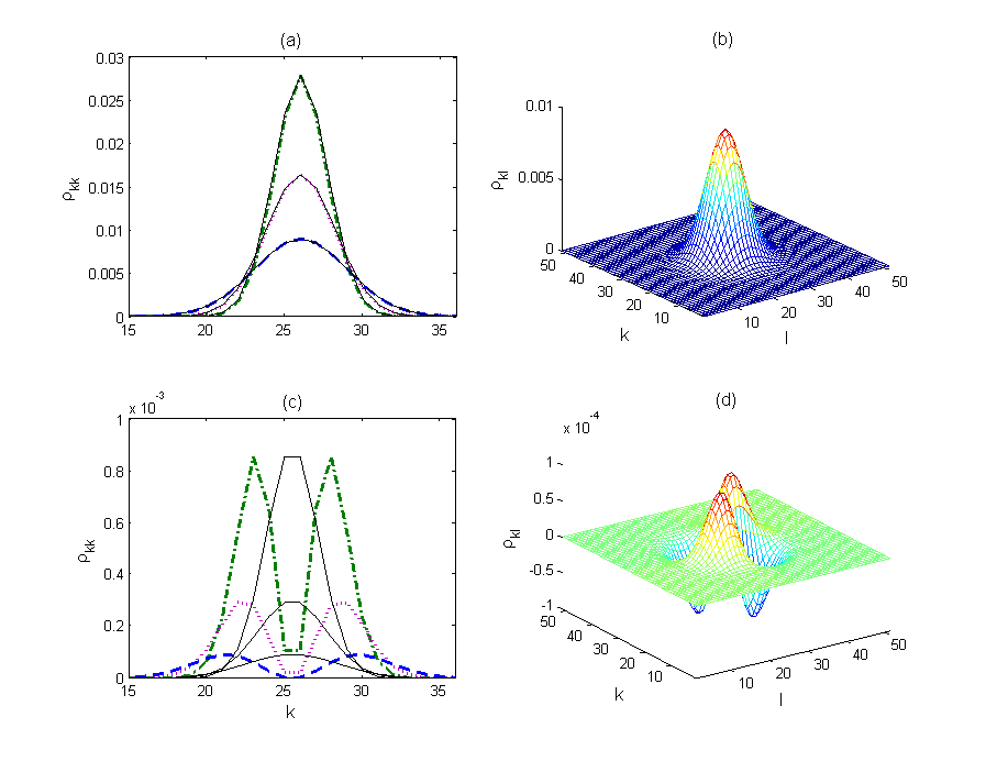
Figure 2: (a) A solution of the master equation Eq. (12) for diagonal elements, $\rho_{kk}$, for only one TLS initially excited (the one in the middle of the chain, $j=26$). Dash-dotted, dotted and dashed curves correspond to the times $\gamma t=3,5,9$. Thin solid lines depict results Eq. (19) given by the heat equation. (b) A solution of Eq. (12) for all elements, $\rho_{kl}$, for only one TLS initially excited ($j=26$); $\gamma t=9$. (c) Solutions of Eq.(12) for diagonal elements, $\rho_{kk}$, for completely entangled initial states $\rho_{\pm}$ (24). Dash-dotted, dotted and dashed curves correspond to the times $\gamma t=3,5,9$ for the initial state $\rho_{-}$, $j=25$. Thin solid lines correspond to the same times for the initial state $\rho_{+}$. For comparison, solutions are normalized. (d) A solution of Eq. (12) for all elements, $\rho_{kl}$, for the initial state $\rho_{+}$, $j=25$; $\gamma t=9$. For all examples the number of TLS in the chain is $N=51$.

3 Single-excitation equations

To clarify essential features of dynamics prescribed by the master equation (1), let us consider the initial chain state confined to the single-excitation subspace. Then, as follows from Eq.(1), the single-excitation matrix elements,

$$\rho_{kl}=\langle 1_{k}|\rho|1_{l}\rangle,$$

satisfy the following equation:

$$\frac{d}{dt}\rho_{kl}=-(\gamma_{k}+\gamma_{k-1}+\gamma_{l}+\gamma_{l-1})\rho_{kl}+$$

$$\qquad\quad\gamma_{k}\rho_{k+1,l}+\gamma_{k-1}\rho_{k-1,l}+\gamma_{l}\rho_{k,l+1}+\gamma_{l-1}\rho_{k,l-1},$$ (12)

where the relaxation rates, $\gamma_{k}$, are defined in accordance with conditions (2). Away from the edges, Eq. (12) coincides with a standard equation for a discrete classical random walk in two dimensions in continuous time, and describes diffusive propagation of the excitation through the chain mediated by emission to reservoirs and re-absorption from them [28].

As follows from Eq.(1), the coherences between the single-excitation subspace and the vacuum

$$\rho_{k0}=\langle 1_{k}|\rho|0\rangle,\quad|0\rangle=\prod\limits_{k=1}^{N+1}|-_{k}\rangle$$

satisfy the standard classical equation for the one-dimensional discrete classical random walk:

$$\frac{d}{dt}\rho_{k0}=-(\gamma_{k}+\gamma_{k-1})\rho_{k0}+\gamma_{k}\rho_{k+1,0}+\gamma_{k-1}\rho_{k-1,0}.$$ (13)

The immediate consequence of the classical form of both Eqs. (12) and (13) is the conservation of sums of corresponding matrix elements:

$$W=\sum\limits_{k,l=1}^{N+1}\rho_{kl}(t)=\sum\limits_{k,l=1}^{N+1}\rho_{kl}(0),$$

$$F=\sum\limits_{k=1}^{N+1}\rho_{k0}(t)=\sum\limits_{k=1}^{N+1}\rho_{k0}(0).$$ (14)

Eqs.(14) are a consequence of collective character of coupling to reservoirs. The chain described by the master equation (1) has another pure stationary state in addition to the usual lowest-energy one. This state satisfies the equation $S_{j}^{-}|\Psi\rangle=0$, for all $j$. It is a pure and an entangled state. It describes the equal superposition of single-excitation states. For a chain with $N+1$ elements this state is

$$|\Psi\rangle=\frac{1}{\sqrt{N+1}}\sum_{j=1}^{N+1}|1_{j}\rangle,$$ (15)

where

$$|1_{j}\rangle=|+_{j}\rangle\prod\limits_{k\neq j}|-_{k}\rangle.$$

So, the state (15) describes just one excitation "spread" homogeneously over all the systems of the chain.

Eqs. (12) and (13) can be easily solved analytically [44]. For example, the solution for the elements $\rho_{kl}(t)$ can be written as

$$\rho_{kl}(t)=\sum\limits_{m,n=1}^{N+1}\alpha^{kl}_{mn}\exp\{-\lambda_{m,n}t\},$$ (16)

where the eigenvalues for Eq. (12) are

$$\lambda_{m,n}=4\gamma\left\{\sin^{2}\left(\frac{\pi m}{N+1}\right)+\sin^{2}\left(\frac{\pi n}{N+1}\right)\right\}.$$

The coefficients $\alpha^{kl}_{mn}$ are defined from the initial state:

$$\alpha^{kl}_{mn}={\nu_{km}\nu_{ln}}\langle\Phi_{m}|\rho(0)|\Phi_{n}\rangle,$$

where the coefficients are

$$\nu_{km}=\sqrt{(2-\delta_{k,N+1})}\cos\left(\frac{2\pi k}{N+1}m\right).$$

The symbol $\delta_{ij}$ denotes Kronecker delta, and the vectors are

$$|\Phi_{l}\rangle=\frac{1}{\sqrt{N+1}}\sum\limits_{n=1}^{N+1}\nu_{ln}|1_{n}\rangle.$$ (17)

Vectors (17) are mutually orthogonal, $\langle\Phi_{m}|\Phi_{n}\rangle=\delta_{mn}$. However, they do not diagonalize the density matrix, $\rho$. Since $\lambda_{N+1,N+1}=0$, the vector $|\Phi_{N+1}\rangle$ is the stationary state $|\Psi\rangle$, see Eq. (15).

Solution of Eq.(13) is similar to the solution of Eq. (12). Eq. (12) can also be viewed as a discretization of the standard heat-transfer equation in the square $L\times L$, where $L=Na/2$ is the chain length, and $a$ is the doubled distance between neighboring systems in the original chain (the one depicted above in Fig.(1)). The later one can be obtained by assuming $ak\rightarrow x$, $al\rightarrow y$:

$$\frac{d}{dt}\rho(x,y;t)\approx a^{2}\gamma\left(\frac{\partial^{2}\rho(x,y;t)}{\partial x^{2}}+\frac{\partial^{2}\rho(x,y;t)}{\partial y^{2}}\right).$$ (18)

The absence of quantum flux over the chain boundaries corresponds to the Neumann boundary conditions for the density matrix at the square boundaries $x=0,L$ and $y=0,L$. The discrete solution (16) approximate the solution for the Neumann boundary conditions only in the limit $N\rightarrow\infty$. For initial states having only non-negative elements, $\rho_{kl}(t=0)\geq 0$, Eq. (12) gives $\rho_{kl}(t>0)\geq 0$. Thus, elements $\rho_{kl}$ can be taken for classical probabilities, and our dissipatively coupled 1D chain can indeed simulate 2D classical walk or heat transfer. In Fig. 2(a) examples of dynamics are shown for the case of just one TLS being initially completely excited. Even for modest number of TLS in the chain ($N=51$ for our example depicted in Fig. (2)) solutions of Eq. (12) given by Eq.(16) are very close to the fundamental solution of Eq. (18) obtained in the limit of infinitely-length chain

$$\rho_{0}(x,y;t)=\frac{1}{4a^{2}\gamma t}\exp\left\{-[(x-x_{0})^{2}+(y-y_{0})^{2}]/2a^{2}\gamma t\right\},$$ (19)

for $\gamma t>1$. Here $x_{0},y_{0}$ denote the position of the initial excitation.

A continuous approximation for Eq.(13) is the 1D heat-transfer equation,

$$\frac{d}{dt}\rho(z;t)\approx a^{2}\gamma\frac{\partial^{2}\rho(z;t)}{\partial z^{2}}.$$ (20)

All the consideration given above can be extended for this case, too. So, our dissipatively coupled 1D chain can simulate simultaneously both 1D and 2D classical random walk, or heat transfer.

Non-exponential decay in our chain is stipulated by nonlocality of Lindblad operators in Eqs. (12) and (13)). It is interesting and instructive to compare the dynamics of population decay in our chain with dynamics of collective spontaneous emission of dense atomic cloud with dipole-dipole interaction [7, 8]. The continuous limit of master equation correspondent to the model considered in Ref.  [7, 8] is given by Eq.(A) in the A. Eq.(A) looks similar to Eq. (18) and also manifests an algebraic law of population decay, $1/\sqrt{\gamma t}$ [7]. However, it holds in 3D-space, and describes quite different physical process. The reason for it is the formal equivalence of Eq.(A) to the master equation with nonlocal Lindblad operators. This nonlocality arises from non-conservation of the excitation number and from accounting for quantum states corresponding to two excited atoms and one virtual photon with "negative" energy [7].

4 Anomalous heat transfer

Eqs. (12) and (13)) tell us that elements of the density matrix in the energy eigenstates basis evolve according to classical equations. However, despite this fact, the energy flow through the 1D chain cannot be described by the 1D classical Fourier law even in the limit of the large number of TLS in the chain. This holds even in the case, where the density matrix elements of the initial single-excitation state are non-negative. Indeed, as it was shown in the previous Section (see Eqs. (14)), the sum of matrix elements,

$$W=\sum\limits_{k,l=1}^{N+1}\rho_{kl},$$

is preserved. Simultaneously, the total upper-state population of the chain does decay. As it follows from Eqs. (12), for example, for the initial state being just one completely excited TLS, the total population behaves in the following way:

$$\left\langle\sum\limits_{k=1}^{N+1}|1_{k}\rangle\langle 1_{k}|\right\rangle=\sum\limits_{k=1}^{N+1}\rho_{kk}\propto\frac{1}{\sqrt{\gamma t}}.$$

A physical reason for breaking the classical Fourier heat conductivity law is rather simple. Besides the energy transport occurring in one dimension (along the chain), there is an additional motion. Fourier law is always breaking down in presence of additional motions (the simplest example is the convection in liquids [29]). In our case this additional motion is a flow of quantum coherence. Indeed, in the continuous approximation the energy flux along the chain reads as

$$J(x,x)\propto\lim\limits_{y\rightarrow x}\frac{\partial}{\partial x}\rho(x,y;t).$$ (21)

The right-hand part of this equation cannot be represented in the form of the gradient of a scalar function satisfying the 1D heat-transfer equation. Thus, the right-hand part of Eq.(21), or the energy per TLS, $\rho(x,x;t)$, cannot be associated with classical temperature [29]. Since in our chain not only energy is transported, but also quantum coherences, it is possible to introduce the concept of the effective 2D "quantum temperature" and 2D quantum flux as, correspondingly,

$$T_{q}(x,y;t)=\rho(x,y;t),$$

$$\vec{J}_{q}(x,y;t)\propto\nabla_{xy}\rho(x,y;t).$$

The value of the real energy flux corresponds to the $x$-component of quantum flux, $\vec{e}_{x}\cdot\vec{J}_{q}(x,x;t)$, where $\vec{e}_{x}$ is the unit vector along the chain, while the $y$-component describes the coherences transfer. This additional motion produces a second dimension in the heat transfer equation and leads to the anomalous thermodynamics. A number of examples of an anomalous thermodynamical behavior for quantum structures is known (see, for example, Refs.[30, 31, 32]). But the dissipatively coupled chain differs starkly by the nature of anomaly. One can retrieve classical thermodynamics and establish connection between "classical" and "quantum" temperatures by neglecting the additional motions in Eq.(18), i.e. by averaging out some coherences. Indeed, introducing the averaged temperature and averaged energy flux as

$$T_{class}(x;t)=\int\rho(x,y;t)dy,$$ (22)

$$\vec{J}_{class}(x;t)=\int\vec{J}_{q}(x,y;t)dy$$ (23)

one obtains 1D heat transfer equation for temperature and relation between the temperature and energy flux,

$$\vec{J}_{\rm class}(x;t)=\vec{e}_{x}\frac{\partial}{\partial x}T_{\rm class}(x;t),$$

in full agreement with Fourier heat conductivity theory. But there is no convincing reasons for such approximation to be done and for the association of the integrals (22, 23) with a real physical temperature and a real energy flux. As it will be shown below, use of such classical model in our case leads to the disappearance of some important observable regimes.

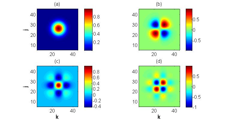
Figure 3: Contour plots of exact solutions of the master equation Eq. (12) for initial states (25). For the panel (a) the initial state is the just one completely excited system, $m=0$. For the panel (b) $m=1$, $f_{0}=f_{1}=1/\sqrt{2}$. For the panel (c) $m=2$, $f_{0}=f_{2}=1/\sqrt{6}$, $f_{1}=2/\sqrt{6}$. For the panel (d) $m=3$, $f_{0}=f_{3}=1/\sqrt{20}$, $f_{1}=f_{2}=3/\sqrt{20}$. For all the panels $\gamma t=9$, $N=51$. For comparison, solutions are normalized (the largest element is taken to be unity).

5 Polynomial decay of populations

The dissipatively coupled chain offers unique possibility of controlling the quantum state dynamics. Just by choosing different initial state, one can manipulate the law of spontaneous decay. Also, dependence of the decay law on the type of initial state gives one an opportunity of identifying initial states of the chain by measuring the population of just one TLS.

We have obtained that for the simple 1D set of TLS coupled to common Markovian reservoirs and the single initially excited TLS, the upper-state population decay for chain TLS occurs polynomially, according the the $1/t$ law. Let us now demonstrate by just adjusting the initial state of the chain, one can obtain a population decay law $1/t^{2m+1}$ for an arbitrary $m\geq 0$. Interestingly, we can arrange initial conditions that are hardly possible in the classical case. In particular, it is possible to create equivalents of neighboring regions with "positive" and "negative" temperatures (or even "imaginary" ones). It can be done by choosing an initial state with components orthogonal to the stationary state (15). An example of $\rho_{kl}$ dynamics for such a state is demonstrated in Fig. 2(c), where the solutions of Eq. (12) are shown for entangled initial states:

$$\rho_{\pm}=|\psi_{\pm}\rangle\langle\psi_{\pm}|,\quad|\psi_{\pm}\rangle=\frac{1}{\sqrt{2}}(|1_{j}\rangle\pm|1_{j+1}\rangle).$$ (24)

The solution for the state $\rho_{+}$ behaves itself "classically": both closely situated initial peaks are soon merged together in one Gaussian shape. However, dynamics with the initial state $\rho_{-}$ is drastically different: negative elements, $\rho_{kl}$, do persist (Fig. 2 (d)), and initially close peaks are distancing from each other with time. Moreover, excitation displacement for the initial state $\rho_{-}$ appears to be faster than for the initial state $\rho_{+}$. Such a difference can be quite simply illustrated with the solution of the continuous approximation (18). The continuous analog of $\rho_{\pm}$ can be represented as

$$\rho_{\pm}(x,y;t=0)\propto\delta(x-x_{0})\delta(y-y_{0})+\delta(x-(x_{0}+a))\delta(y-(y_{0}+a))$$

$$\qquad\pm\delta(x-(x_{0}+a))\delta(y-y_{0})\pm\delta(x-x_{0})\delta(y-(y_{0}+a)),$$

where $\delta(x)$ is the delta-function. It is easy to see that when the excitation has spread for distances $x$, $y$ such that

$$\sqrt{(x-x_{0})^{2}+(y-y_{0})^{2}}\gg a,$$

the solution for the initial state $\rho_{+}$ is given by Eq. (19). However, for the initial state $\rho_{-}$ dynamics is quite different. When the excitation has spread far enough, the solution for the initial state $\rho_{-}$ is

$$\rho(x,y;t)\approx 2\rho_{0}(x,y;t){(x-x_{0})(y-y_{0})}/{(2a\gamma t)^{3}}.$$

Thus, just by choosing the initial state to be $\rho_{-}$, we get the population decay law $1/t^{3}$. This state doesn’t exist within the bounds of quasiclassical Fourier theory. Indeed, the averaging of this state following (22, 23) leads to the trivial solution: the temperature as well as energy flux equal to zero at arbitrary point of space for every moment of time. It is not hard to see that the population decay law can be further varied by choice of the initial state. Let us consider pure initial states of the general form

$$|\phi\rangle=\sum\limits_{i=0}^{m}(-1)^{i}f_{i}|1_{k+i}\rangle,$$ (25)

where $f_{i}$ are some scalar coefficients, and the excitation is assumed to be well localized, $m\ll N$. Taking the continuous approximation and using the quantity $m/\gamma t\ll 1$ as small parameter, from Eq. (25) we straightforwardly obtain the following approximation:

$$\rho(x,y;t)\approx\rho_{0}(x,y;t)\sum\limits_{n=0}^{\infty}\frac{1}{n!(2a^{2}\gamma t)^{n}}$$

$$\times\sum\limits_{i,j=0}^{m}(-1)^{i+j}f_{i}f_{j}[i(x-x_{0})+j(y-y_{0})]^{n}.$$ (26)

Starting with the initial state (25) and choosing the coefficients $f_{i}$ in the form of the normalized binomial coefficients, $f_{i}\propto{m!}/{i!(m-i)!}$, we get the first non-zero term in the approximation (26) of the order of $1/t^{2m+1}$. Examples of exact solutions for initial states (25) are shown in Figs. 3. The panels (a-d) corresponds to $m=0,1,2,3$.

Notice, that the states (25) are non-correctly described within the bounds of the quasiclassical Fourier theory. The "classical" averaging of states (25) as it is done in Eqs. (22, 23) can lead to the drastic deformation of them (for example, the states orthogonal to the stationary state will be reduced to zero by such averaging). Mind that polynomial decay regimes considered here are taking place for times, when initially localized excitation has spread far enough. However, we do not consider here an influence of edges. That is, we limit ourselves to the time intervals satisfying $am<v(t)<aN$, where $v(t)$ is the variance of the distribution $\rho_{kl}(t)$. For example, for the single initially excited TLS this condition reads as $1<\gamma t<N$. An influence of chain edges will be considered in further work.

6 Multi-excitation dynamics

It is easy to surmise from Eq.(1) that there is a profound difference between chain dynamics in cases of one and multiple initial excitations. Indeed, the state with multiple excitations will inevitable decay toward mixture of the stationary state (15) and the vacuum state. Generally, for the initial state with no more than $N$ excitation, equations of density elements corresponding to the $N$-excitation subspace describe $2N$-dimensional classical random walk with losses (see equations for an arbitrary number of initial excitations given in B). However, even in this case one can still model lossless multi-dimensional random walks within some limited period of time and for some specific classes of initial states. Moreover, there are regimes when one can have preservation of coherences, where the chain behaves itself in quite "thermodynamic" way.

Let us illustrate our consideration with the case of no more than two initial excitations in the chain . Two-excitation matrix elements are

$$\rho^{k,l}_{m,n}=\langle 1_{k},1_{l}|\rho|1_{m},1_{n}\rangle,$$

where

$$|1_{k},1_{l}\rangle=|+_{k}\rangle|+_{l}\rangle\prod\limits_{j\neq k,l}|-_{j}\rangle.$$

In difference with Eqs.(12), there are two different kinds of equations for the matrix elements $\rho^{k,l}_{m,n}$. For the elements without neighbouring indexes, i.e. for $k\neq l\pm 1$ and $m\neq n\pm 1$, from Eq.(1) one gets the following system of equations (for the sake of illustration we are giving here equations only for the internal TLS of the chain, i.e. $k,l,m,n\neq 1,N+1$):

$$\frac{1}{\gamma}\frac{d}{dt}\rho^{k,l}_{m,n}=-8\rho^{k,l}_{m,n}+\rho^{k+1,l}_{m,n}+\rho^{k-1,l}_{m,n}$$

$$\qquad+\rho^{k,l-1}_{m,n}+\rho^{k,l+1}_{m,n}+\rho^{k,l}_{m-1,n}$$ (27)

$$\qquad+\rho^{k,l}_{m+1,n}+\rho^{k,l}_{m,n-1}+\rho^{k,l}_{m,n+1}.$$

Obviously, Eq.(27) coincides with the equation for 4D classical random walk and in the continuous limit transforms to the 4D heat-transfer equation.

The situation is quite different for the matrix elements with neighbouring indexes. Let us assume, for example, that $l=k+1$. Then, instead of Eqs.(27) one has

$$\frac{1}{\gamma}\frac{d}{dt}\rho^{k,k+1}_{m,n}=-8\rho^{k,k+1}_{m,n}+\rho^{k-1,k+1}_{m,n}+\rho^{k,k+2}_{m,n}$$

$$\qquad+\rho^{k,l}_{m-1,n}+\rho^{k,l}_{m+1,n}+\rho^{k,l}_{m,n-1}+\rho^{k,l}_{m,n+1}.$$ (28)

Eq.(28) does not coincide with the equation for classical random walk. It contains terms describing loss. It can be easily seen in the continuous limit, since then, for example, one has

$$\rho^{k,k+2}_{m,n}-\rho^{k,k+1}_{m,n}\rightarrow\lim\limits_{x_{2}\rightarrow x_{1}}a\frac{\partial}{\partial x_{2}}\rho(x_{1},x_{2},y,z;t),$$

where variables $x_{1},x_{2},y,z$ correspond to the indexes $k,l,m,n$, respectively. Of course, it should be expected. Multi-excitation state does decay toward the single-excitation one.

Eqs. (27) and (28) point to a number of quite counter-intuitive conclusions. First of all, if the initially excited TLS are far from each other, the spread of coherences occurs as for lossless multi-dimensional random walk till the excitation spreads to neighbouring TLS. Notice, that it will take place even in the case of entangled initial state of several TLS. If one has initially several uncorrelated excited TLS being far from another, the whole chain behaves like a set of unconnected chains with just one excitation per chain till the excitation spreads to neighbouring TLS. So, it means that one might have a sort of conservation of coherences in this case, too.

Let us demonstrate an appearance of such a "conservation law of a sorts" with the example of two initially non-interacting chains with no more that one excitation in each. So, we take that there are chains of $M$ and $N$ TLS with both $M,N\gg 1$. Also, corresponding sums of coherences (14), denoted as $W_{M}$ and $W_{N}$ are supposed to be much less than number of TLS, $W_{X}\ll X$, $X=M,N$. We assume that the chains are initially in the stationary states,

$$\rho_{X}^{st}=\frac{W_{X}}{X}|\Psi_{X}\rangle\langle\Psi_{X}|+\left(1-\frac{W_{X}}{X}\right)|V_{X}\rangle\langle V_{X}|,$$ (29)

where $X=M,N$, the vectors $|\Psi_{X}\rangle$ are given by Eq.(15) and vectors $|V_{X}\rangle$ describe the lowest energy state of corresponding chains.

Now let us assume that the chains are coupled by the common dissipative reservoir connecting the last TLS of the first chain and the first TLS of the second chain (the rate of decay to this reservoir we take to be the same $\gamma$ as the rates for all other reservoirs). Then, the stationary state of compound chain will be obviously given also by Eq.(29) with $X=M+N$. It is easy to get from Eqs.(27) and (28) that the sum of coherences for the new stationary state is

$$W_{N+M}=W_{N}+W_{M}+O\left(W_{N}W_{M}\left(\frac{1}{M}+\frac{1}{N}\right)\right)\approx W_{N}+W_{M}.$$ (30)

Notice that the expression (30) becomes exact in the limit $M,N\rightarrow\infty$. So, the sum of coherences for the stationary state of the compound chain is indeed approximately equal to the same of coherences of parts. Moreover, if one disconnects chains and they settle into stationary states again, the value of matrix elements of single-excitation density matrix (the "quantum temperature" as introduced in the Section 4) for both part will remain to be equal, $\rho^{X}_{kl}=(W_{M+N}/(M+N)^{2})$.

7 Conclusions

We have suggested and discussed a tight-binding dissipatively coupled quantum chain. It consists of two-level systems pairwise coupled to the same Markovian reservoirs. We have shown that despite being composed of a comparatively few systems forming the simplest one-dimensional chain, such a chain can model a multi-dimensional random walk, or model a solution of multi-dimensional heat-transfer equation. In difference to the classical "original", it is possible to model heat flow from initial distributions with regions of positive and negative temperatures. Such possibility of quantum stimulations in many-body physics corresponds to the long-standing idea first proposed by R. Feinman and recently cited by C. Cohen-Tannoudji and D. Guery-Odelin as a conclusive remark to their book [3]. This model exhibits anomalous thermodynamics behavior, such as non-Fourier heat conductivity and non-existence of temperature in the classical meaning. The population dynamics of all TLS in the chain is always non-exponential and exhibit polynomial character. By the choice of the initial state, different power laws of decay, $1/t^{2m+1}$, for an arbitrary $m>0$ can be achieved. The suggested chain can be used as an efficient simulator of classically hard problems, such as multi-dimensional quantum walks or heat-transfer equations. Note, that the considered chain is not unique. One can build a number of different dissipatively coupled chains, for example, by changing phases in the system-system interaction terms in the chain.

G. S. acknowledges support from the EU FP7 projects FP7 People 2009 IRSES 247007 CACOMEL and FP7 People 2013 IRSES 612285 CANTOR. This work was also supported by the National Academy of Sciences of Belarus through the program "Convergence", by the External Fellowship Program of the Russian Quantum Center at Skolkovo (D. M., S. K. and E. G.) and by FAPESP grant 2014/21188-0 (D. M.), N. K. and D. M. acknowledge the support provided by the Scottish Universities Physics Alliance (SUPA). The research leading to these results has received funding from the European Community Seventh Framework Programme (FP7/2007-2013) under grant agreement n. 270843 (iQIT). Authors are thankful to Dr. B. W. Lovett, Dr. Sh. Starobinets and Prof. Miguel A. Martin-Delgado for helpful discussions and pointing to relevant references.

References

Appendix A Comparison of dissipatevely coupled quantum chain with spontaneously emitted atomic cloud

It is interesting and constructive to compare single-excitation dynamics of the dissipatively coupled quantum chain with collective spontaneous emission in the dense atomic cloud with dipole-dipole interactions (see Ref.[8]). In [8] in the main text a system of $N$ TLS is considered. Initially, one of them is in the excited state, while all others are in the ground state. TLS are placed at positions $\vec{r}_{j}$, $j=1,2\ldots N$. Multi-mode electromagnetic field is interacting with all TLS. Initially, this field is in the vacuum state, $|vac\rangle$. The solution of the Schrodinger equation for the atoms and field can be represented as

$$|\Psi(t)\rangle=\sum\limits_{j=1}^{N}\beta_{j}(t)|1_{j}\rangle|vac\rangle+|\Psi_{rest}(t)\rangle,$$ (31)

where the coefficients $\beta_{j}(t)$ are amplitudes of having $j$th TLS completely excited; the wave function $|\Psi_{rest}(t)\rangle$ denote components of the total wave function, $|\Psi(t)\rangle$, having other then single excited TLS and the field vacuum. Notice that in Ref. [8] of the main text the rotating-wave approximation was not used to describe TLS-field interaction. So, the function $|\Psi_{rest}(t)\rangle$ includes also components with the number of excitations larger than one.

Using standard approximations about the reservoir, in Ref. [8] the following system of equations was obtained

$$\frac{d}{dt}\beta_{j}(t)=-\gamma\beta_{j}(t)+i\gamma\sum\limits_{k\neq j}\beta_{k}(t)K_{jk},$$ (32)

$$K_{jk}=\frac{\exp\{-ik_{0}|\vec{r}_{k}-\vec{r}_{j}|\}}{k_{0}|\vec{r}_{k}-\vec{r}_{j}|},$$ (33)

where $k_{0}=\omega_{0}/c$, $\omega_{0}$ is the TLS transition frequency, $\gamma$ is the decay rate into the field reservoir.

Eq.(32) can be easily transformed to the form similar to Eq.(12) of the main text. Indeed, introducing the matrix elements $\rho_{jk}=\beta_{j}\beta_{k}^{*}$, from Eq. (32) it follows that

$$\frac{d}{dt}\rho_{jk}=-2\gamma\rho_{jk}+i\gamma\left(\sum\limits_{l\neq j}\rho_{jl}K_{jl}-\sum\limits_{l\neq k}\rho_{lk}K_{lk}^{*}\right).$$

Continuous analog of Eq. (A) reads

$$\frac{d}{dt}\rho(\vec{r},\grave{\vec{r}})=-2\gamma\rho(\vec{r},\grave{\vec{r}})$$

$$\qquad+i\gamma\frac{N}{V}\int\limits_{V}d^{3}\vec{R}\frac{\exp\{-ik_{0}|\vec{r}-\vec{R}|\}}{k_{0}|\vec{r}-\vec{R}|}\rho(\vec{R},\grave{\vec{r}})$$ (34)

$$\qquad-i\gamma\frac{N}{V}\int\limits_{V}d^{3}\vec{R}\frac{\exp\{ik_{0}|\grave{\vec{r}}-\vec{R}|\}}{k_{0}|\grave{\vec{r}}-\vec{R}|}\rho(\vec{r},\vec{R}),$$

where $V$ is the volume of the cloud. Equations Eq.(A), Eq.(A) are similar to the Eqs. (12), (26), respectively. The difference consists in the form of operators in right-hand parts (integral operators with the Green function of Helmholz equation in the capacity of kernel in Eq.(A) instead of Laplace operator in Eq.(26). Integral operators in Eq.(A) are non-Hermitian due to the presence of counter-rotating terms in Eq.(32) which are stipulated by the virtual photons with "negative" energy. It lead to the matrix elements (33) instead of

$$K_{jk}=i\frac{\sin\{k_{0}|\vec{r}_{k}-\vec{r}_{j}|\}}{k_{0}|\vec{r}_{k}-\vec{r}_{j}|}$$ (35)

As a result, Eq (A) is not of Liouville type. It is equal (as Eq. (26) in the main text) to the master equation with non-local Linblad operators. However, it describes rather different physical process. Thus, as it was shown in Ref.[8] in the main text, collective spontaneous emission manifests for some types of boundary conditions algebraic law of population decay. Such behavior is stipulated by the virtual photons with "negative" energy and disappears in the rotation-wave approximation (done by replacing Eq. (33) with Eq.(35)).

Appendix B Equations for the matrix elements for the case of multiple excitations

Here we write down equations for matrix elements corresponding to states with the highest possible number of excitations. Let us assume that initially we have no more than $m$ excitations in the chain (for example, $m$ TLS in completely excited state). From Eq.(1) it is not hard to obtain the following set of equations for the matrix elements corresponding to $m$-excitation subspace

$$\frac{d}{dt}\langle m_{k_{1},k_{2},\ldots,k_{m}}|\rho|m_{l_{1},l_{2},\ldots,l_{m}}\rangle=\sum_{i=1}^{N+1}\lambda_{i}+\mu_{i},$$ (36)

where

$$\lambda_{i}=\{\gamma_{k_{i}}(\langle m_{\{k_{j}+\delta_{j,i}\}}|-\langle m_{\{k_{j}\}}|)$$

$$\qquad+\gamma_{k_{i-1}}(\langle m_{\{k_{j}-\delta_{j,i}\}}|-\langle m_{\{k_{j}\}}|)\}\rho|m_{\{l_{i}\}}\rangle,$$ (37)

$$\mu_{i}=\langle m_{\{k_{i}\}}|\rho\{\gamma_{l_{i}}(|m_{\{l_{j}+\delta_{j,i}\}}\rangle-|m_{\{l_{j}\}}\rangle)$$

$$\qquad+\gamma_{l_{i}-1}(|m_{\{l_{j}-\delta_{j,i}\}}\rangle-|m_{\{l_{j}\}}\rangle)\}.$$

Here the state $|m_{\{l_{j}\}}\rangle=|m_{l_{1},l_{2},\ldots,l_{m}}\rangle$ is the state with $m$ TLS with numbers $l_{1},l_{2},\ldots,l_{m}$ being completely excited. Also, $|m_{\{l_{j}\pm\delta_{j,i}\}}\rangle=|m_{l_{1},l_{2},\ldots,l_{i}\pm 1,\ldots,l_{m}}\rangle$. As it is in Eq.(3) of the main body of the paper, we are assuming that $\gamma_{0}\equiv 0$, and $\gamma_{k>0}\equiv\gamma$. Notice that in case when the indexes are neighbors, i.e. when $k_{i+1}=k_{i}+1$, one has

$$\lambda_{i}=-\gamma_{k_{i}}\langle m_{\{k_{j}\}}|\rho|m_{\{l_{i}\}}\rangle+$$

$$\qquad\gamma_{k_{i-1}}\langle m_{\{k_{j}-\delta_{j,i}\}}|\rho|m_{\{l_{i}\}}\rangle-\langle m_{\{k_{j}\}}|\rho|m_{\{l_{i}\}}\rangle,$$

$$\lambda_{i+1}=\gamma_{k_{i+1}}\langle m_{\{k_{j}+\delta_{j,i+1}\}}|\rho|m_{\{l_{i}\}}\rangle-$$

$$\qquad\gamma_{k_{i+1}}\langle m_{\{k_{j}\}}|\rho|m_{\{l_{i}\}}\rangle-\gamma_{k_{i}}\langle m_{\{k_{j}\}}|\rho|m_{\{l_{i}\}}\rangle.$$

The same holds for the case of neighboring $l_{i}$ and $l_{i+1}$. For indexes equal to $1$ or $N+1$ corresponding $\lambda$s are

$$\lambda_{1}=\gamma_{k_{1}}(\langle m_{k_{1}+1,k_{2},...,k_{m}}|-\langle m_{k_{1},k_{2},...,k_{m}}|)|\rho|m_{\{l_{i}\}}\rangle,$$

$$\lambda_{N+1}=\gamma_{k_{N}}(\langle m_{k_{1},k_{2},...,k_{m}-1}|-\langle m_{k_{1},k_{2},...,k_{m}}|)|\rho|m_{\{l_{i}\}}\rangle.$$

For matrix elements without neighboring excitations, i.e. $k_{i}\neq k_{j}\pm 1$, $l_{i}\neq l_{j}\pm 1$, $\forall k_{i},k_{j}$, one obtains that Eq.(36) is the discretization of the following $2m$-dimensional heat-transfer equation

$$\frac{d}{dt}\rho(\{x_{k}\},\{y_{k}\};t)\approx a^{2}\gamma\sum_{k=1}^{m}\frac{\partial^{2}\rho(\{x_{k}\},\{y_{k}\};t)}{\partial x_{k}^{2}}$$

$$\qquad\qquad+a^{2}\gamma\sum_{k=1}^{m}\frac{\partial^{2}\rho(\{x_{k}\},\{y_{k}\};t)}{\partial y_{k}^{2}}.$$ (38)

References

- [1] J. Hubbard, Proc. of the Royal Society of London 276, 238 (1963).
- [2] E. Ising, Z.Physik, 31, 253 (1925).
- [3] C. Cohen-Tannoudji and D. Guery-Odelin, Advances in Atomic Physics: an Overview, World Scientific Publishing Ltd, New-Jersey, 2011.
- [4] J.Q. You, F. Nori, Nature 474, 589 (2011).
- [5] M. O. Scully and M. S. Zubairy, Quantum Optics Cambridge University Press, Cambridge, UK, 1997.
- [6] D. Jaksch, D. C. Bruder, J. Cirac, C. Gardiner, P. Zoller, Phys. Rev. Lett. 81 3108 (1998).
- [7] M. O. Scully, Phys. Rev. Lett. 102, 143601 (2009).
- [8] A. A. Svidzinsky, J.-T.Chang, and M. O. Scully, Phys. Rev. A81, 053821 (2010).
- [9] S. Schmidt and G. Blatter, Phys. Rev. Lett. 103, 086403 (2009).
- [10] J. O. Owens, M. A. Broome, D. N. Biggerstaff, M. E. Goggin, A. Fedrizzi, T. Linjordet, M. Ams, G. D. Marshall, J. Twamley, M. J. Withford and A. G. White, New J. Phys. 13 075003 (2011).
- [11] M. Michel, G. Mahler, and J. Gemmer, Phys. Rev. Lett. 95, 180602 (2005).
- [12] Y. Dubi and M. Di Ventra, Phys. Rev. E79 042101 (2009).
- [13] R. Rohlsberger, K. Schlage, B. Sahoo, S. Couet, R. Ruffer, Science 328 1248 (2010).
- [14] G. Y. Slepyan, Y. Yerchak, A. Hoffmann, and F. G. Bass, Phys. Rev. B81, 085115 (2010).
- [15] G. Y. Slepyan, Y. Yerchak, S. A. Maksimenko, A. Hoffmann, and F. G .Bass, Phys. Rev.B85, 245134 (2012).
- [16] S. Bose, Phys. Rev. Lett. 91, 207901 (2003).
- [17] G. Y. Slepyan and A. Boag, Phys. Rev. Lett, 111, 023602 (2013).
- [18] D. A. Lidar, I. L. Chuang, and K. B. Whaley, Phys. Rev. Lett. 81, 2594(1998).
- [19] P. G. Kwiat, A. J. Berglund, J. B. Altepeter, A. G. White, Science 290, 498-501 (2000).
- [20] D. Braun, Phys. Rev. Lett. 89, 277901 (2002).
- [21] Guo-Yong Xiang, Zhi-Bo Hou, Chuan-Feng Li, Guang-Can Guo, Heinz-Peter Breuer, Elsi-Mari Laine, Jyrki Piilo, arXiv:1401.5091 [quant-ph] (2014).
- [22] V. S. Shchesnovich, D. S. Mogilevtsev, Phys. Rev. A 82, 043621 (2010).
- [23] D. Mogilevtsev and V. S. Shchesnovich, Optt. Lett. 35, 3375 (2010).
- [24] A. Mikhalychev, D. Mogilevtsev, S. Kilin, Journal of Physics A: Mathematical and Theoretical, 8 12 (2011).
- [25] D. Mogilevtsev, A. Mikhalychev, V.S. Shchesnovich, N. Korolkova, Phys.Rev. A87, 063847 (2013).
- [26] A. Rivas, O. Viyuela and M. A. Martin-Delgado, Phys. Rev. B 88, 155141 (2013).
- [27] Y. Ping, B. W. Lovett, S. C. Benjamin, and E. M. Gauger, Phys. Rev. Lett. 110, 100503 (2013).
- [28] J. Kempe, Contemporary Physics 44, 307 (2003).
- [29] L. D. Landau and E. M. Lifshitz, Fluid Mechanics, Course of Theoretical Physics, Vol. 6, (Pergamon Ltd. book, 1985).
- [30] S. G. Volz, Phys. Rev. Lett. 87,074301 (2001).
- [31] Y. Dubi and M. Di Ventra, Rev. Mod. Phys. 83, 131(2011).
- [32] A. Celani, S. Bo, R. Eichhorn, and E. Aurell, Phys. Rev. Lett. 109, 260603(2012).
- [33] M. S. Rudner and L. S. Levitov, Phys. Rev. Lett. 102, 065703 (2009).
- [34] H.-P. Breuer and F. Petruccione, The Theory of Open Quantum Systems, Oxford University Press (2007).
- [35] F. Jelezko and J. Wrachtrup, Phys. Stat. Sol. A203, 3207 (2006).
- [36] E. Rittweger, Kyu Young Han, S. E. Irvine, Ch. Eggeling and S. W. Hell, Nature Phot. 3, 144 (2009).
- [37] A. A. Khajetoorians, J. Wiebe, B. Chilian, R. Wiesendanger, Science 332, 1062 (2011).
- [38] A. A. Khajetoorians, B. Baxevanis, Ch. Hübner, T. Schlenk, S. Krause, T.O. Wehling, S. Lounis, A. Lichtenstein, D. Pfannkuche, J. Wiebe, R. Wiesendanger, Science 339, 55 (2013).
- [39] A. A. Khajetoorians, T. Schlenk, B. Schweflinghaus, M. dos Santos Dias, M. Steinbrecher, M. Bouhassoune, S. Lounis, J. Wiebe and R. Wiesendanger, Phys. Rev. Lett. 111, 157204 (2013).
- [40] H. Friedenauer, H. Schmitz, J. T. Glueckert, D. Porras and T. Schaetz, Nat. Phys. 4 757 (2008).
- [41] M. Enderlein, Th. Huber, Ch. Schneider, and T. Schaetz, Phys. Rev. Lett. 109, 233004 (2012).
- [42] A. W. Chin, A. Datta, F. Caruso, S. F. Huelga, and M. B. Plenio, New J. Phys. 12 065002 (2010).
- [43] J. Strumpfer and K. Schulten, J. Chem. Phys. 134, 095102 (2011).
- [44] G. F. Lawler Random Walk and the Heat Equation (Student Mathematical Library), American Mathematical Society (2010).