Quantized Minimax Estimation
over Sobolev Ellipsoids

Abstract

We formulate the notion of minimax estimation under storage or communication constraints, and prove an extension to Pinsker’s theorem for nonparametric estimation over Sobolev ellipsoids. Placing limits on the number of bits used to encode any estimator, we give tight lower and upper bounds on the excess risk due to quantization in terms of the number of bits, the signal size, and the noise level. This establishes the Pareto optimal tradeoff between storage and risk under quantization constraints for Sobolev spaces. Our results and proof techniques combine elements of rate distortion theory and minimax analysis. The proposed quantized estimation scheme, which shows achievability of the lower bounds, is adaptive in the usual statistical sense, achieving the optimal quantized minimax rate without knowledge of the smoothness parameter of the Sobolev space. It is also adaptive in a computational sense, as it constructs the code only after observing the data, to dynamically allocate more codewords to blocks where the estimated signal size is large. Simulations are included that illustrate the effect of quantization on statistical risk. nonparametric estimation, minimax bounds, rate distortion theory, constrained estimation, Sobolev ellipsoid

1 Introduction

In this paper we introduce a minimax framework for nonparametric estimation under storage constraints. In the classical statistical setting, the minimax risk for estimating a function $f$ from a function class ${\mathcal{F}}$ using a sample of size $n$ places no constraints on the estimator ${\widehat{f}_{n}}$, other than requiring it to be a measurable function of the data. However, if the estimator is to be constructed with restrictions on the computational resources used, it is of interest to understand how the error can degrade. Letting $C(\widehat{f}_{n})\leq B_{n}$ indicate that the computational resources $C(\widehat{f}_{n})$ used to construct $\widehat{f}_{n}$ are required to fall within a budget $B_{n}$, the constrained minimax risk is

$$R_{n}({\mathcal{F}},B_{n})=\inf_{\widehat{f}_{n}:C(\widehat{f}_{n})\leq B_{n}}\sup_{f\in{\mathcal{F}}}R(\widehat{f}_{n},f).$$

Minimax lower bounds on the risk as a function of the computational budget thus determine a feasible region for computation constrained estimation, and a Pareto optimal tradeoff for risk versus computation as $B_{n}$ varies.

Several recent papers have presented results on tradeoffs between statistical risk and computational resources, measured in terms of either running time of the algorithm, number of floating point operations, or number of bits used to store or construct the estimators [6, 5, 16]. However, the existing work quantifies the tradeoff by analyzing the statistical and computational performance of specific procedures, rather than by establishing lower bounds and a Pareto optimal tradeoff. In this paper we treat the case where the complexity $C(\widehat{f}_{n})$ is measured by the storage or space used by the procedure and sharply characterize the optimal tradeoff. Specifically, we limit the number of bits used to represent the estimator $\widehat{f}_{n}$. We focus on the setting of nonparametric regression under standard smoothness assumptions, and study how the excess risk depends on the storage budget $B_{n}$.

We view the study of quantized estimation as a theoretical problem of fundamental interest. But quantization may arise naturally in future applications of large scale statistical estimation. For instance, when data are collected and analyzed on board a remote satellite, the estimated values may need to be sent back to Earth for further analysis. To limit communication costs, the estimates can be quantized, and it becomes important to understand what, in principle, is lost in terms of statistical risk through quantization. A related scenario is a cloud computing environment where data are processed for many different statistical estimation problems, with the estimates then stored for future analysis. To limit the storage costs, which could dominate the compute costs in many scenarios, it is of interest to quantize the estimates, and the quantization-risk tradeoff again becomes an important concern. Estimates are always quantized to some degree in practice. But to impose energy constraints on computation, future processors may limit precision in arithmetic computations more significantly [11]; the cost of limited precision in terms of statistical risk must then be quantified. A related problem is to distribute the estimation over many parallel processors, and to then limit the communication costs of the submodels to the central host. We focus on the centralized setting in the current paper, but an extension to the distributed case may be possible with the techniques that we introduce here.

We study risk-storage tradeoffs in the normal means model of nonparametric estimation assuming the target function lies in a Sobolev space. The problem is intimately related to classical rate distortion theory [12], and our results rely on a marriage of minimax theory and rate distortion ideas. We thus build on and refine the connection between function estimation and lossy source coding that was elucidated in David Donoho’s 1997 Wald Lectures [9].

We work in the Gaussian white noise model

$$dX(t)=f(t)dt+\varepsilon dW(t),\quad 0\leq t\leq 1,$$ (1.1)

where $W$ is a standard Wiener process on $[0,1]$, $\varepsilon$ is the standard deviation of the noise, and $f$ lies in the periodic Sobolev space $\widetilde{W}(m,c)$ of order $m$ and radius $c$. (We discuss the nonperiodic Sobolev space $W(m,c)$ in Section 4.) The white noise model is a centerpiece of nonparametric estimation. It is asymptotically equivalent to nonparametric regression [4] and density estimation [18], and simplifies some of the mathematical analysis in our framework. In this classical setting, the minimax risk of estimation

$$R_{\varepsilon}(m,c)=\inf_{\widehat{f}_{\varepsilon}}\sup_{f\in\widetilde{W}(m,c)}\mathbb{E}\,\|f-\widehat{f}_{\varepsilon}\|_{2}^{2}$$

is well known to satisfy

$$\lim_{\varepsilon\to 0}\varepsilon^{-\frac{4m}{2m+1}}R_{\varepsilon}(m,c)=\left(\frac{c^{2}(2m+1)}{\pi^{2m}}\right)^{\frac{1}{2m+1}}\left(\frac{m}{m+1}\right)^{\frac{2m}{2m+1}}\triangleq\mathsf{P}_{m,c}$$ (1.2)

where $\mathsf{P}_{m,c}$ is Pinsker’s constant [19]. The constrained minimax risk for quantized estimation becomes

$$R_{\varepsilon}(m,c,B_{\varepsilon})=\inf_{\widehat{f}_{\varepsilon},C(\widehat{f}_{\varepsilon})\leq B_{\varepsilon}}\sup_{f\in\widetilde{W}(m,c)}\mathbb{E}\,\|f-\widehat{f}_{\varepsilon}\|_{2}^{2}$$

where $\widehat{f}_{\varepsilon}$ is a quantized estimator that is required to use storage $C(\widehat{f}_{\varepsilon})$ no greater than $B_{\varepsilon}$ bits in total. Our main result identifies three separate quantization regimes.

• In the over-sufficient regime, the number of bits is very large, satisfying $B_{\varepsilon}\gg\varepsilon^{-\frac{2}{2m+1}}$ and the classical minimax rate of convergence $R_{\varepsilon}\asymp\varepsilon^{\frac{4m}{2m+1}}$ is obtained. Moreover, the optimal constant is the Pinsker constant ${\mathsf{P}}_{m,c}$.

• In the sufficient regime, the number of bits scales as $B_{\varepsilon}\asymp\varepsilon^{-\frac{2}{2m+1}}$. This level of quantization is just sufficient to preserve the classical minimax rate of convergence, and thus in this regime $R_{\varepsilon}(m,c,B_{\varepsilon})\asymp\varepsilon^{\frac{4m}{2m+1}}$. However, the optimal constant degrades to a new constant ${\mathsf{P}}_{m,c}+{\mathsf{Q}}_{m,c,d}$, where ${\mathsf{Q}}_{m,c,d}$ is characterized in terms of the solution of a certain variational problem, depending on $d=\lim_{\varepsilon\rightarrow 0}B_{\varepsilon}\varepsilon^{\frac{2}{2m+1}}$.

• In the insufficient regime, the number of bits scales as $B_{\varepsilon}\ll\varepsilon^{-\frac{2}{2m+1}}$, with however $B_{\varepsilon}\to\infty$. Under this scaling the number of bits is insufficient to preserve the unquantized minimax rate of convergence, and the quantization error dominates the estimation error. We show that the quantized minimax risk in this case satisfies

  $$\lim_{\varepsilon\to 0}B_{\varepsilon}^{2m}R_{\varepsilon}(m,c,B_{\varepsilon})=\frac{c^{2}m^{2m}}{\pi^{2m}}.$$

  Thus, in the insufficient regime the quantized minimax rate of convergence is $B_{\varepsilon}^{-2m}$, with optimal constant as shown above.

By using an upper bound for the family of constants ${\mathsf{Q}}_{m,c,d}$, the three regimes can be combined together to view the risk in terms of a decomposition into estimation error and quantization error. Specifically, we can write

$$R_{\varepsilon}(m,c,B_{\varepsilon})\;\;\approx\underbrace{\mathsf{P}_{m,c}\,\varepsilon^{\frac{4m}{2m+1}}}_{\mbox{\footnotesize estimation error}}+\underbrace{\frac{c^{2}m^{2m}}{\pi^{2m}}B_{\varepsilon}^{-2m}}_{\mbox{\footnotesize quantization error}}.$$

When $B_{\varepsilon}\gg\varepsilon^{-\frac{2}{2m+1}}$, the estimation error dominates the quantization error, and the usual minimax rate and constant are obtained. In the insufficient case $B_{\varepsilon}\ll\varepsilon^{-\frac{2}{2m+1}}$, only a slower rate of convergence is achievable. When $B_{\varepsilon}$ and $\varepsilon^{-\frac{2}{2m+1}}$ are comparable, the estimation error and quantization error are on the same order. The threshold $\varepsilon^{-\frac{2}{2m+1}}$ should not be surprising, given that in classical unquantized estimation the minimax rate of convergence is achieved by estimating the first $\varepsilon^{-\frac{2}{2m+1}}$ Fourier coefficients and simply setting the remaining coefficients to zero. This corresponds to selecting a smoothing bandwidth that scales as $h\asymp n^{-\frac{1}{2m+1}}$ with the sample size $n$.

At a high level, our proof strategy integrates elements of minimax theory and source coding theory. In minimax analysis one computes lower bounds by thinking in Bayesian terms to look for least-favorable priors. In source coding analysis one constructs worst case distributions by setting up an optimization problem based on mutual information. Our quantized minimax analysis requires that these approaches be carefully combined to balance the estimation and quantization errors. To show achievability of the lower bounds we establish, we likewise need to construct an estimator and coding scheme together. Our approach is to quantize the blockwise James-Stein estimator, which achieves the classical Pinsker bound. However, our quantization scheme differs from the approach taken in classical rate distortion theory, where the generation of the codebook is determined once the source distribution is known. In our setting, we require the allocation of bits to be adaptive to the data, using more bits for blocks that have larger signal size. We therefore design a quantized estimation procedure that adaptively distributes the communication budget across the blocks. Assuming only a lower bound $m_{0}$ on the smoothness $m$ and an upper bound $c_{0}$ on the radius $c$ of the Sobolev space, our quantization-estimation procedure is adaptive to $m$ and $c$ in the usual statistical sense, and is also adaptive to the coding regime. In other words, given a storage budget $B_{\varepsilon}$, the coding procedure achieves the optimal rate and constant for the unknown $m$ and $c$, operating in the corresponding regime for those parameters.

In the following section we establish some notation, outline our proof strategy, and present some simple examples. In Section 3 we state and prove our main result on quantized minimax lower bounds, relegating some of the technical details to an appendix. In Section 4 we show asymptotic achievability of these lower bounds, using a quantized estimation procedure based on adaptive James-Stein estimation and quantization in blocks, again deferring proofs of technical lemmas to the supplementary material. This is followed by a presentation of some results from experiments in Section 5, illustrating the performance and properties of the proposed quantized estimation procedure.

2 Quantized estimation and minimax risk

Suppose that $(X_{1},\dots,X_{n})\in\mathcal{X}^{n}$ is a random vector drawn from a distribution $P_{n}$. Consider the problem of estimating a functional $\theta_{n}=\theta(P_{n})$ of the distribution, assuming $\theta_{n}$ is restricted to lie in a parameter space $\Theta_{n}$. To unclutter some of the notation, we will suppress the subscript $n$ and write $\theta$ and $\Theta$ in the following, keeping in mind that nonparametric settings are allowed. The subscript $n$ will be maintained for random variables. The minimax $\ell_{2}$ risk of estimating $\theta$ is then defined as

$$R_{n}(\Theta)=\inf_{\widehat{\theta}_{n}}\sup_{\theta\in\Theta}\mathbb{E}_{\theta}\|\theta-\widehat{\theta}_{n}\|^{2}$$

where the infimum is taken over all possible estimators $\widehat{\theta}_{n}:\mathcal{X}^{n}\to\Theta$ that are measurable with respect to the data $X_{1},\dots,X_{n}$. We will abuse notation by using $\widehat{\theta}_{n}$ to denote both the estimator and the estimate calculated based on an observed set of data. Among numerous approaches to obtaining the minimax risk, the Bayesian method is best aligned with quantized estimation. Consider a prior distribution $\pi(\theta)$ whose support is a subset of $\Theta$. Let $\delta(X_{1:n})$ be the posterior mean of $\theta$ given the data $X_{1},\dots,X_{n}$, which minimizes the integrated risk. Then for any estimator $\widehat{\theta}_{n}$,

$$\sup_{\theta\in\Theta}\mathbb{E}_{\theta}\|\theta-\widehat{\theta}_{n}\|^{2}\geq\int_{\Theta}\mathbb{E}_{\theta}\|\theta-\widehat{\theta}_{n}\|^{2}d\pi(\theta)\geq\int_{\Theta}\mathbb{E}_{\theta}\|\theta-\delta(X_{1:n})\|^{2}d\pi(\theta).$$

Taking the infimum over $\widehat{\theta}_{n}$ yields

$$\inf_{\widehat{\theta}_{n}}\sup_{\theta\in\Theta}\mathbb{E}_{\theta}\|\theta-\widehat{\theta}_{n}\|^{2}\geq\int_{\Theta}\mathbb{E}_{\theta}\|\theta-\delta(X_{1:n})\|^{2}d\pi(\theta)\triangleq R_{n}(\Theta;\pi).$$

Thus, any prior distribution supported on $\Theta$ gives a lower bound on the minimax risk, and selecting the least-favorable prior leads to the largest lower bound provable by this approach.

Now consider constraints on the storage or communication cost of our estimate. We restrict to the set of estimators that use no more than a total of $B_{n}$ bits; that is, the estimator takes at most $2^{B_{n}}$ different values. Such quantized estimators can be formulated by the following two-step procedure. First, an encoder maps the data $X_{1:n}$ to an index $\phi_{n}(X_{1:n})$, where

$$\phi_{n}:\mathbb{\mathcal{X}}^{n}\to\{1,2,\dots,2^{B_{n}}\}$$

is the encoding function. The decoder, after receiving or retrieving the index, represents the estimates based on a decoding function

$$\psi_{n}:\{1,2,\dots,2^{B_{n}}\}\to\Theta,$$

mapping the index to a codebook of estimates. All that needs to be transmitted or stored is the $B_{n}$-bit-long index, and the quantized estimator $\widehat{\theta}_{n}$ is simply $\psi_{n}\circ\phi_{n}$, the composition of the encoder and the decoder functions. Denoting by $C(\widehat{\theta}_{n})$ the storage, in terms of the number of bits, required by an estimator $\widehat{\theta}_{n}$, the minimax risk of quantized estimation is then defined as

$$R_{n}(\Theta,B_{n})=\inf_{\widehat{\theta}_{n},C(\widehat{\theta}_{n})\leq B_{n}}\sup_{\theta\in\Theta}\mathbb{E}_{\theta}\|\theta-\widehat{\theta}_{n}\|^{2},$$

and we are interested in the effect of the constraint on the minimax risk. Once again, we consider a prior distribution $\pi(\theta)$ supported on $\Theta$ and let $\delta(X_{1:n})$ be the posterior mean of $\theta$ given the data. The integrated risk can then be decomposed as

$$\int_{\Theta}\mathbb{E}_{\theta}\|\theta-\widehat{\theta}_{n}\|^{2}d\pi(\theta) =\mathbb{E}\|\theta-\delta(X_{1:n})+\delta(X_{1:n})-\widehat{\theta}_{n}\|^{2}$$ (2.1)

$$=\mathbb{E}\|\theta-\delta(X_{1:n})\|^{2}+\mathbb{E}\|\delta(X_{1:n})-\widehat{\theta}_{n}\|^{2}$$

where the expectation is with respect to the joint distribution of $\theta\sim\pi(\theta)$ and $X_{1:n}\,|\,\theta\sim P_{\theta}$, and the second equality is due to

$$\mathbb{E}\langle\theta-\delta(X_{1:n}),\delta(X_{1:n})-\widehat{\theta}_{n}\rangle$$

$$=\mathbb{E}\left(\mathbb{E}\left(\langle\theta-\delta(X_{1:n}),\delta(X_{1:n})-\widehat{\theta}_{n}\rangle\,|\,X_{1:n}\right)\right)$$

$$=\mathbb{E}\left(\langle\mathbb{E}(\theta-\delta(X_{1:n})\,|\,X_{1:n}),\delta(X_{1:n})-\widehat{\theta}_{n}\rangle\right)$$

$$=\mathbb{E}\left(\langle 0,\delta(X_{1:n})-\widehat{\theta}_{n}\rangle\right)=0,$$

using the fact that $\theta\to X_{1:n}\to\widehat{\theta}_{n}$ forms a Markov chain. The first term in the decomposition (2.1) is the Bayes risk $R_{n}(\Theta;\pi)$. The second term can be viewed as the excess risk due to quantization.

Let $T_{n}=T(X_{1},\dots,X_{n})$ be a sufficient statistic for $\theta$. The posterior mean can be expressed in terms of $T_{n}$ and we will abuse notation and write it as $\delta(T_{n})$. Since the quantized estimator $\widehat{\theta}_{n}$ uses at most $B_{n}$ bits, we have

$$B_{n}\geq H(\widehat{\theta}_{n})\geq H(\widehat{\theta}_{n})-H(\widehat{\theta}_{n}\,|\,\delta(T_{n}))=I(\widehat{\theta}_{n};\delta(T_{n})),$$

where $H$ and $I$ denote the Shannon entropy and mutual information, respectively. Now consider the optimization

$$\inf_{P(\cdot\,|\,\delta(T_{n}))}\ \ \mathbb{E}\|\delta(T_{n})-\widetilde{\theta}_{n}\|^{2}$$

such that $$\ I(\widetilde{\theta}_{n};\delta(T_{n}))\leq B_{n}$$

where the infimum is over all conditional distributions $P(\widetilde{\theta}_{n}\,|\,\delta(T_{n}))$. This parallels the definition of the distortion rate function, minimizing the distortion under a constraint on mutual information [12]. Denoting the value of this optimization by $Q_{n}(\Theta,B_{n};\pi)$, we can lower bound the quantized minimax risk by

$$R_{n}(\Theta,B_{n})\geq R_{n}(\Theta;\pi)+Q_{n}(\Theta,B_{n};\pi).$$

Since each prior distribution $\pi(\theta)$ supported on $\Theta$ gives a lower bound, we have

$$R_{n}(\Theta,B_{n})\geq\sup_{\pi}\Bigl{\{}R_{n}(\Theta;\pi)+Q_{n}(\Theta,B_{n};\pi)\Bigr{\}}$$

and the goal becomes to obtain a least favorable prior for the quantized risk.

Before turning to the case of quantized estimation over Sobolev spaces, we illustrate this technique on some simpler, more concrete examples.

Example 2.1 (Normal means in a hypercube).

Let $X_{i}\sim\mathcal{N}(\theta,\sigma^{2}I_{d})$ for $i=1,2,\dots,n$. Suppose that $\sigma^{2}$ is known and $\theta\in[-\tau,\tau]^{d}$ is to be estimated. We choose the prior $\pi(\theta)$ on $\theta$ to be a product distribution with density

$$\pi(\theta)=\prod_{j=1}^{d}\frac{3}{2\tau^{3}}{\left(\tau-|\theta_{j}|\right)_{+}}^{2}.$$

It is shown in [15] that

$$R_{n}(\Theta;\pi)\geq\frac{\sigma^{2}d}{n}\frac{\tau^{2}}{\tau^{2}+12\sigma^{2}/n}\geq c_{1}\frac{\sigma^{2}d}{n}$$

where $c_{1}=\frac{\tau^{2}}{\tau^{2}+12\sigma^{2}}$. Turning to $Q_{n}(\Theta,B_{n};\pi)$, let $T^{(n)}=(T^{(n)}_{1},\dots,T^{(n)}_{d})=\mathbb{E}(\theta|X_{1:n})$ be the posterior mean of $\theta$. In fact, by the independence and symmetry among the dimensions, we know $T_{1},\dots,T_{d}$ are independently and identically distributed. Denoting by $T_{0}^{(n)}$ this common distribution, we have

$$Q_{n}(\Theta,B_{n};\pi)\geq d\cdot q(B_{n}/d)$$

where $q(B)$ is the distortion rate function for $T^{(n)}_{0}$, i.e., the value of the following problem

$$\inf_{P(\widehat{T}\,|\,T_{0}^{(n)})}\ \ \mathbb{E}(T_{0}^{(n)}-\widehat{T})^{2}$$

such that $$\ I(\widehat{T};T_{0}^{(n)})\leq B.$$

Now using the Shannon lower bound [8], we get

$$Q_{n}(\Theta,B_{n};\pi)\geq\frac{d}{2\pi e}\cdot 2^{h(T_{0}^{(n)})}\cdot 2^{-\frac{2B_{n}}{d}}.$$

Note that as $n\to\infty$, $T_{0}^{(n)}$ converges to $\theta$ in distribution, so there exists a constant $c_{2}$ independent of $n$ and $d$ such that

$$R_{n}(\Theta,B_{n})\geq c_{1}\frac{\sigma^{2}d}{n}+c_{2}d\,2^{-\frac{2B_{n}}{d}}.$$

This lower bound intuitively shows the risk is regulated by two factors, the estimation error and the quantization error; whichever is larger dominates the risk. The scaling behavior of this lower bound (ignoring constants) can be achieved by first quantizing each of the $d$ intervals $[-\tau,\tau]$ using $B_{n}/d$ bits each, and then mapping the mle to its closest codeword.

Example 2.2 (Gaussian sequences in Euclidean balls).

In the example shown above, the lower bound is tight only in terms of the scaling of the key parameters. In some instances, we are able to find an asymptotically tight lower bound for which we can show achievability of both the rate and the constants. Estimating the mean vector of a Gaussian sequence with an $\ell_{2}$ norm constraint on the mean is one of such case, as we showed in previous work [27].

Specifically, let $X_{i}\sim\mathcal{N}(\theta_{i},\sigma^{2}_{n})$ for $i=1,2,\ldots,n$, where $\sigma^{2}_{n}=\sigma^{2}/n$. Suppose that the parameter $\theta=(\theta_{1},\ldots,\theta_{n})$ lies in the Euclidean ball $\Theta_{n}(c)=\left\{\theta:\sum_{i=1}^{n}\theta_{i}^{2}\leq c^{2}\right\}$. Furthermore, suppose that $B_{n}=nB$. Then using the prior $\theta_{i}\sim\mathcal{N}(0,c^{2})$ it can be shown that

$$\liminf_{n\to\infty}R_{n}(\Theta_{n}(c),B_{n})\geq\frac{\sigma^{2}c^{2}}{\sigma^{2}+c^{2}}+\frac{c^{4}2^{-2B}}{\sigma^{2}+c^{2}}.$$

The asymptotic estimation error $\sigma^{2}c^{2}/(\sigma^{2}+c^{2})$ is the well-known Pinsker bound for the Euclidean ball case. As shown in [27], an explicit quantization scheme can be constructed that asymptotically achieves this lower bound, realizing the smallest possible quantization error $c^{4}2^{-2B}/(\sigma^{2}+c^{2})$ for a budget of $B_{n}=nB$ bits.

The Euclidean ball case is clearly relevant to the Sobolev ellipsoid case, but new coding strategies and proof techniques are required. In particular, as will be made clear in the sequel, we will use an adaptive allocation of bits across blocks of coefficients, using more bits for blocks that have larger estimated signal size. Moreover, determination of the optimal constants requires a detailed analysis of the worst case prior distributions and the solution of a series of variational problems.

3 Quantized estimation over Sobolev spaces

Recall that the Sobolev space of order $m$ and radius $c$ is defined by

$$W(m,c)=\Big{\{} f\in[0,1]\to\mathbb{R}:f^{(m-1)}\text{ is absolutely continuous and }$$

$$\int_{0}^{1}(f^{(m)}(x))^{2}dx\leq c^{2}\Big{\}}.$$

The periodic Sobolev space is defined by

$$\widetilde{W}(m,c)=\left\{f\in W(m,c):f^{(j)}(0)=f^{(j)}(1),\ j=0,1,\dots,m-1\right\}.$$ (3.1)

The white noise model (1.1) is asymptotically equivalent to making $n$ equally spaced observations along the sample path, $Y_{i}=f(i/n)+\sigma\epsilon_{i}$, where $\epsilon_{i}\sim{\mathcal{N}}(0,1)$ [4]. In this formulation, the noise level in the formulation (1.1) scales as $\epsilon^{2}=\sigma^{2}/n$, and the rate of convergence takes the familiar form $n^{-\frac{2m}{2m+1}}$ where $n$ is the number of observations.

To carry out quantized estimation we now require an encoder

$$\phi_{\varepsilon}:\mathbb{R}^{[0,1]}\to\{1,2,\dots,2^{B_{\varepsilon}}\}$$

which is a function applied to the sample path $X(t)$. The decoding function then takes the form

$$\psi_{\varepsilon}:\{1,2,\dots,2^{B_{\varepsilon}}\}\to\mathbb{R}^{[0,1]}$$

and maps the index to a function estimate. As in the previous section, we write the composition of the encoder and the decoder as $\widehat{f}_{\varepsilon}=\psi_{\varepsilon}\circ\phi_{\varepsilon}$, which we call the quantized estimator. The communication or storage $C(\widehat{f}_{\varepsilon})$ required by this quantized estimator is no more than $B_{\varepsilon}$ bits.

To recast quantized estimation in terms of an infinite sequence model, let $({\varphi_{j}})_{j=1}^{\infty}$ be the trigonometric basis, and let

$$\theta_{j}=\int_{0}^{1}\varphi_{j}(t)f(t)dt,\quad j=1,2,\dots,$$

be the Fourier coefficients. It is well known [22] that $f=\sum_{j=1}^{\infty}\theta_{j}\varphi_{j}$ belongs to $\widetilde{W}(m,c)$ if and only if the Fourier coefficients $\theta$ belong to the Sobolev ellipsoid defined as

$$\Theta(m,c)=\left\{\theta\in\ell_{2}:\sum_{j=1}^{\infty}a_{j}^{2}\theta_{j}^{2}\leq\frac{c^{2}}{\pi^{2m}}\right\}$$ (3.2)

where

$$a_{j}=\begin{cases}j^{m},&\text{for even }j,\\ (j-1)^{m},&\text{for odd }j.\end{cases}$$

Although this is the standard definition of a Sobolev ellipsoid, for the rest of the paper we will set $a_{j}=j^{m}$, $j=1,2,\dots$ for convenience of analysis. All of the results hold for both definitions of $a_{j}$. Also note that (3.2) actually gives a more general definition, since $m$ is no longer assumed to be an integer, as it is in (3.1). Expanding with respect to the same orthonormal basis, the observed path $X(t)$ is converted into an infinite Gaussian sequence

$$Y_{j}=\int_{0}^{1}\varphi_{j}(t)\,dX(t),\quad j=1,2,\dots,$$

with $Y_{j}\sim\mathcal{N}(\theta_{j},\varepsilon^{2})$. For an estimator $(\widehat{\theta}_{j})_{j=1}^{\infty}$ of $(Y_{j})_{j=1}^{\infty}$, an estimate of $f$ is obtained by

$$\widehat{f}(x)=\sum_{j=1}^{\infty}\widehat{\theta}_{j}\varphi_{j}(x)$$

with squared error $\|\widehat{f}-f\|_{2}^{2}=\|\widehat{\theta}-\theta\|_{2}^{2}$. In terms of this standard reduction, the quantized minimax risk is thus reformulated as

$$R_{\varepsilon}(m,c,B_{\varepsilon})=\inf_{\widehat{\theta}_{\varepsilon},C(\widehat{\theta}_{\varepsilon})\leq B_{\varepsilon}}\sup_{\theta\in\Theta(m,c)}\mathbb{E}\,_{\theta}\|\theta-\widehat{\theta}_{\varepsilon}\|_{2}^{2}.$$ (3.3)

To state our result, we need to define the value of the following variational problem:

$${\mathsf{V}}_{m,c,d}\triangleq$$ (3.4)

$$\max_{(\sigma^{2},x_{0})\in{\mathcal{F}}(m,c,d)}\int_{0}^{x_{0}}\frac{\sigma^{2}(x)}{\sigma^{2}(x)+1}dx+x_{0}\exp\left(\frac{1}{x_{0}}\int_{0}^{x_{0}}\log\frac{\sigma^{4}(x)}{\sigma^{2}(x)+1}dx-\frac{2d}{x_{0}}\right)$$

where the feasible set ${\mathcal{F}}(m,c,d)$ is the collection of increasing functions $\sigma^{2}(x)$ and values $x_{0}$ satisfying

$$\int_{0}^{x_{0}}x^{2m}\sigma^{2}(x)dx\leq c^{2}$$

$$\frac{\sigma^{4}(x)}{\sigma^{2}(x)+1}\geq\exp\left(\frac{1}{x_{0}}\int_{0}^{x_{0}}\log\frac{\sigma^{4}(x)}{\sigma^{2}(x)+1}dx-\frac{2d}{x_{0}}\right)\text{ for all }x\leq x_{0}.$$

The significance and interpretation of the variational problem will become apparent as we outline the proof of this result.

Theorem 3.1.

Let $R_{\varepsilon}(m,c,B_{\varepsilon})$ be defined as in (3.3), for $m>0$ and $c>0$.

1. If $B_{\varepsilon}\varepsilon^{\frac{2}{2m+1}}\to\infty$ as $\varepsilon\to 0$, then

   $$\liminf_{\varepsilon\to 0}\varepsilon^{-\frac{4m}{2m+1}}R_{\varepsilon}(m,c,B_{\varepsilon})\geq\mathsf{P}_{m,c}$$

   where $\mathsf{P}_{m,c}$ is Pinker’s constant defined in (1.2).

2. If $B_{\varepsilon}\varepsilon^{\frac{2}{2m+1}}\to d$ for some constant $d$ as $\varepsilon\to 0$, then

   $$\liminf_{\varepsilon\to 0}\varepsilon^{-\frac{4m}{2m+1}}R_{\varepsilon}(m,c,B_{\varepsilon})\geq\mathsf{P}_{m,c}+\mathsf{Q}_{m,c,d}={\mathsf{V}}_{m,c,d}$$

   where $\mathsf{V}_{m,c,d}$ is the value of the variational problem (3.4).

3. If $B_{\varepsilon}\varepsilon^{\frac{2}{2m+1}}\to 0$ and $B_{\varepsilon}\to\infty$ as $\varepsilon\to 0$, then

   $$\liminf_{\varepsilon\to 0}B_{\varepsilon}^{2m}R_{\varepsilon}(m,c,B_{\varepsilon})\geq\frac{c^{2}m^{2m}}{\pi^{2m}}.$$

In the first regime where the number of bits $B_{\varepsilon}$ is much greater than $\varepsilon^{-\frac{2}{2m+1}}$, we recover the same convergence result as in Pinsker’s theorem, in terms of both convergence rate and leading constant. The proof of the lower bound for this regime can directly follow the proof of Pinsker’s theorem, since the set of estimators considered in our minimax framework is a subset of all possible estimators.

In the second regime where we have “just enough” bits to preserve the rate, we suffer a loss in terms of the leading constant. In this “Goldilocks regime,” the optimal rate $\varepsilon^{-\frac{4m}{2m+1}}$ is achieved but the constant in front of the rate is Pinsker’s constant $\mathsf{P}_{m,c}$ plus a positive quantity $\mathsf{Q}_{m,c,d}$ determined by the variational problem.

While the solution to this variational problem does not appear to have an explicit form, it can be computed numerically. We discuss this term at length in the sequel, where we explain the origin of the variational problem, compute the constant numerically and approximate it from above and below. The constants $\mathsf{P}_{m,c}$ and $\mathsf{Q}_{m,c,d}$ are shown graphically in Figure 1. Note that the parameter $d$ can be thought of as the average number of bits per coefficient used by an optimal quantized estimator, since $\varepsilon^{-\frac{2}{2m+1}}$ is asymptotically the number of coefficients needed to estimate at the classical minimax rate. As shown in Figure 1, the constant for quantized estimation quickly approaches the Pinsker constant as $d$ increases—when $d=3$ the two are already very close.

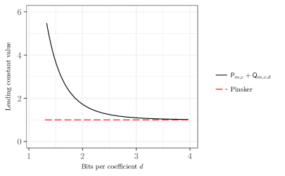
Figure 1: The constants $\mathsf{P}_{m,c}+\mathsf{Q}_{m,c,d}$ as a function of quantization level $d$ in the sufficient regime, where $B_{\varepsilon}\varepsilon^{\frac{2}{2m+1}}\to d$. The parameter $d$ can be thought of as the average number of bits per coefficient used by an optimal quantized estimator, because $\varepsilon^{-\frac{2}{2m+1}}$ is asymptotically the number of coefficients needed to estimate at the classical minimax rate. Here we take $m=2$ and $c^{2}/\pi^{2m}=1$. The curve indicates that with only $2$ bits per coefficient, optimal quantized minimax estimation degrades by less than a factor of 2 in the constant. With $3$ bits per coefficient, the constant is very close to the classical Pinsker constant.

In the third regime where the communication budget is insufficient for the estimator to achieve the optimal rate, we obtain a sub-optimal rate which no longer depends explicitly on the noise level $\varepsilon$ of the model. In this regime, quantization error dominates, and the risk decays at a rate of $B^{-\frac{1}{2m}}$ no matter how fast $\varepsilon$ approaches zero, as long as $B\ll\varepsilon^{-\frac{2}{2m+1}}$. Here the analogue of Pinsker’s constant takes a very simple form.

Proof of Theorem 3.1.

Consider a Gaussian prior distribution on $\theta=(\theta_{j})_{j=1}^{\infty}$ with $\theta_{j}\sim\mathcal{N}(0,\sigma_{j}^{2})$ for $j=1,2,\dots,$ in terms of parameters $\sigma^{2}=(\sigma_{j}^{2})_{j=1}^{\infty}$ to be specified later. One requirement for the variances is

$$\sum_{j=1}^{\infty}a_{j}^{2}\sigma_{j}^{2}\leq\frac{c^{2}}{\pi^{2m}}.$$

We denote this prior distribution by $\pi(\theta;\sigma^{2})$, and show in Section A that it is asymptotically concentrated on the ellipsoid $\Theta(m,c)$. Under this prior the model is

$$\theta_{j} \sim\mathcal{N}(0,\sigma_{j}^{2})$$

$$Y_{j}\,|\,\theta_{j} \sim\mathcal{N}(\theta_{j},\varepsilon^{2}),\quad j=1,2,\dots$$

and the marginal distribution of $Y_{j}$ is thus ${\mathcal{N}}(0,\sigma^{2}_{j}+\varepsilon^{2})$. Following the strategy outlined in Section 2, let $\delta$ denote the posterior mean of $\theta$ given $Y$ under this prior, and consider the optimization

$$\quad\inf\ \ \mathbb{E}\|\delta-\widetilde{\theta}\|^{2}$$

such that $$\ I(\delta;\widetilde{\theta})\leq B_{\epsilon}$$

where the infimum is over all distributions on $\widetilde{\theta}$ such that $\theta\to Y\to\widetilde{\theta}$ forms a Markov chain. Now, the posterior mean satisfies $\delta_{j}=\gamma_{j}Y_{j}$ where $\gamma_{j}=\sigma_{j}^{2}/(\sigma_{j}^{2}+\epsilon^{2})$. Note that the Bayes risk under this prior is

$$\mathbb{E}\,\|\theta-\delta\|_{2}^{2}=\sum_{j=1}^{\infty}\frac{\sigma_{j}^{2}\varepsilon^{2}}{\sigma_{j}^{2}+\varepsilon^{2}}.$$

Define

$$\mu_{j}^{2}\triangleq\mathbb{E}\,(\delta_{j}-\widetilde{\theta}_{j})^{2}.$$

Then the classical rate distortion argument [8] gives that

$$I(\delta;\widetilde{\theta}) \geq\sum_{j=1}^{\infty}I(\gamma_{j}Y_{j};\widetilde{\theta}_{j})$$

$$\geq\sum_{j=1}^{\infty}\frac{1}{2}\log_{+}\left(\frac{\gamma_{j}^{2}(\sigma^{2}_{j}+\varepsilon^{2})}{\mu_{j}^{2}}\right)$$

$$=\sum_{j=1}^{\infty}\frac{1}{2}\log_{+}\left(\frac{\sigma_{j}^{4}}{\mu_{j}^{2}(\sigma_{j}^{2}+\varepsilon^{2})}\right)$$

where $\log_{+}(x)=\max(\log x,0)$. Therefore, the quantized minimax risk is lower bounded by

$$R_{\varepsilon}(m,c,B_{\varepsilon})=\inf_{\widehat{\theta}_{\varepsilon},C(\widehat{\theta}_{\varepsilon})\leq B_{\varepsilon}}\sup_{\theta\in\Theta(m,c)}\mathbb{E}\|\theta-\widehat{\theta}_{\varepsilon}\|^{2}\geq V_{\varepsilon}(B_{\varepsilon},m,c)(1+o(1))$$

where $V_{\varepsilon}(B_{\varepsilon},m,c)$ is the value of the optimization

$$\max_{\sigma^{2}}\min_{\mu^{2}} \ \sum_{j=1}^{\infty}\mu_{j}^{2}+\sum_{j=1}^{\infty}\frac{\sigma_{j}^{2}\varepsilon^{2}}{\sigma_{j}^{2}+\varepsilon^{2}} \mathcal{P}_{1}$$ ()

such that $$\ \sum_{j=1}^{\infty}\frac{1}{2}\log_{+}\left(\frac{\sigma_{j}^{4}}{\mu_{j}^{2}(\sigma_{j}^{2}+\varepsilon^{2})}\right)\leq B_{\varepsilon}$$

$$\ \sum_{j=1}^{\infty}a_{j}^{2}\sigma_{j}^{2}\leq\frac{c^{2}}{\pi^{2m}}$$

and the $(1+o(1))$ deviation term is analyzed in the supplementary material.

Observe that the quantity $V_{\varepsilon}(B_{\varepsilon},m,c)$ can be upper and lower bounded by

$$\max\Bigl{\{}R_{\varepsilon}(m,c),Q_{\varepsilon}(m,c,B_{\varepsilon})\Bigr{\}}\leq V_{\varepsilon}(m,c,B_{\varepsilon})\\ \leq R_{\varepsilon}(m,c)+Q_{\varepsilon}(m,c,B_{\varepsilon})$$ (3.5)

where the estimation error term $R_{\varepsilon}(m,c)$ is the value of the optimization

$$\max_{\sigma^{2}} \ \sum_{j=1}^{\infty}\frac{\sigma_{j}^{2}\varepsilon^{2}}{\sigma_{j}^{2}+\varepsilon^{2}} \mathcal{R}_{1}$$ ()

such that $$\ \sum_{j=1}^{\infty}a_{j}^{2}\sigma_{j}^{2}\leq\frac{c^{2}}{\pi^{2m}}$$

and the quantization error term $Q_{\varepsilon}(m,c,B_{\varepsilon})$ is the value of the optimization

$$\max_{\sigma^{2}}\min_{\mu^{2}} \ \sum_{j=1}^{\infty}\mu_{j}^{2} \mathcal{Q}_{1}$$ ()

such that $$\ \sum_{j=1}^{\infty}\frac{1}{2}\log_{+}\left(\frac{\sigma_{j}^{4}}{\mu_{j}^{2}(\sigma_{j}^{2}+\varepsilon^{2})}\right)\leq B_{\varepsilon}$$

$$\ \sum_{j=1}^{\infty}a_{j}^{2}\sigma_{j}^{2}\leq\frac{c^{2}}{\pi^{2m}}.$$

The following results specify the leading order asymptotics of these quantities.

Lemma 3.1.

As $\varepsilon\to 0$,

$$R_{\varepsilon}(m,c)=\mathsf{P}_{m,c}\,\varepsilon^{\frac{4m}{2m+1}}(1+o(1)).$$

Lemma 3.2.

As $\varepsilon\to 0$,

$$Q_{\varepsilon}(m,c,B_{\varepsilon})\leq\frac{c^{2}m^{2m}}{\pi^{2m}}B_{\varepsilon}^{-2m}(1+o(1)).$$ (3.6)

Moreover, if $B_{\varepsilon}\varepsilon^{\frac{2}{2m+1}}\to 0$ and $B_{\varepsilon}\to\infty$,

$$Q_{\varepsilon}(m,c,B_{\varepsilon})=\frac{c^{2}m^{2m}}{\pi^{2m}}B_{\varepsilon}^{-2m}(1+o(1)).$$

This yields the following closed form upper bound.

Corollary 3.1.

Suppose that $B_{\varepsilon}\to\infty$ and $\varepsilon\to 0$. Then

$$V_{\varepsilon}(m,c,B_{\varepsilon})\leq\left(\mathsf{P}_{m,c}\,\varepsilon^{\frac{4m}{2m+1}}+\frac{c^{2}m^{2m}}{\pi^{2m}}B_{\varepsilon}^{-2m}\right)(1+o(1)).$$ (3.7)

In the insufficient regime $B_{\varepsilon}\varepsilon^{\frac{2}{2m+1}}\to 0$ and $B_{\varepsilon}\to\infty$ as $\varepsilon\to 0$, equation (3.5) and Lemma 3.2 show that

$$V_{\varepsilon}(m,c,B_{\varepsilon})=\frac{c^{2}m^{2m}}{\pi^{2m}}B_{\varepsilon}^{-2m}(1+o(1)).$$

Similarly, in the over-sufficient regime $B_{\varepsilon}\varepsilon^{\frac{2}{2m+1}}\to\infty$ as $\varepsilon\to 0$, we conclude that

$$V_{\varepsilon}(m,c,B_{\varepsilon})=\mathsf{P}_{m,c}\,\varepsilon^{\frac{4m}{2m+1}}(1+o(1)).$$

We now turn to the sufficient regime $B_{\varepsilon}\varepsilon^{\frac{2}{2m+1}}\to d$. We begin by making three observations about the solution to the optimization ($\mathcal{P}_{1}$). First, we note that the series $(\sigma^{2}_{j})_{j=1}^{\infty}$ that solves ($\mathcal{P}_{1}$) can be assumed to be decreasing. If $(\sigma^{2}_{j})$ were not in decreasing order, we could rearrange it to be decreasing, and correspondingly rearrange $(\mu^{2}_{j})$, without violating the constraints or changing the value of the optimization. Second, we note that given $(\sigma^{2}_{j})$, the optimal $(\mu^{2}_{j})$ is obtained by the “reverse water-filling” scheme [8]. Specifically, there exists $\eta>0$ such that

$$\mu_{j}^{2}=\begin{cases}\eta&\text{ if }\displaystyle\frac{\sigma_{j}^{4}}{\sigma_{j}^{2}+\varepsilon^{2}}\geq\eta\\ \displaystyle\frac{\sigma_{j}^{4}}{\sigma_{j}^{2}+\varepsilon^{2}}&\text{ otherwise},\end{cases}$$

where $\eta$ is chosen so that

$$\frac{1}{2}\sum_{j=1}^{\infty}\log_{+}\left(\frac{\sigma_{j}^{4}}{\mu_{j}^{2}(\sigma_{j}^{2}+\varepsilon^{2})}\right)\leq B_{\varepsilon}.$$

Third, there exists an integer $J>0$ such that the optimal series $(\sigma^{2}_{j})$ satisfies

$$\frac{\sigma_{j}^{4}}{\sigma^{2}_{j}+\varepsilon^{2}}\geq\eta,\text{ for }j=1,\dots,J\quad\text{and}\quad\sigma_{j}^{2}=0,\text{ for }j>J,$$

where $\eta$ is the “water-filling level” for $(\mu^{2}_{j})$ (see [8]). Using these three observations, the optimization ($\mathcal{P}_{1}$) can be reformulated as

$$\max_{\sigma^{2},J} \ J\eta+\sum_{j=1}^{J}\frac{\sigma_{j}^{2}\varepsilon^{2}}{\sigma_{j}^{2}+\varepsilon^{2}} \mathcal{P}_{2}$$ ()

such that $$\ \frac{1}{2}\sum_{j=1}^{J}\log_{+}\left(\frac{\sigma_{j}^{4}}{\eta(\sigma_{j}^{2}+\varepsilon^{2})}\right)=B_{\varepsilon}$$

$$\ \sum_{j=1}^{J}a_{j}^{2}\sigma_{j}^{2}\leq\frac{c^{2}}{\pi^{2m}}$$

$$\ (\sigma_{j}^{2})\text{ is decreasing and }\frac{\sigma_{J}^{4}}{\sigma_{J}^{2}+\varepsilon^{2}}\geq\eta.$$

To derive the solution to ($\mathcal{P}_{2}$), we use a continuous approximation of $\sigma^{2}$, writing

$$\sigma^{2}_{j}=\sigma^{2}(jh)h^{2m+1}$$

where $h$ is the bandwidth to be specified and $\sigma^{2}(\cdot)$ is a function defined on $(0,\infty)$. The constraint that $\sum_{j=1}^{\infty}a_{j}^{2}\sigma^{2}_{j}\leq\frac{c^{2}}{\pi^{2m}}$ becomes the integral constraint [19]

$$\int_{0}^{\infty}x^{2m}\sigma^{2}(x)dx\leq\frac{c^{2}}{\pi^{2m}}.$$

We now set the bandwidth so that $h^{2m+1}=\varepsilon^{2}$. This choice of bandwidth will balance the two terms in the objective function, and thus gives the hardest prior distribution. Applying the above three observations under this continuous approximation, we transform problem ($\mathcal{P}_{2}$) to the following optimization:

$$\quad\max_{\sigma^{2},x_{0}} \ x_{0}\eta+\int_{0}^{x_{0}}\frac{\sigma^{2}(x)}{\sigma^{2}(x)+1}dx \mathcal{P}_{3}$$ ()

such that $$\ \int_{0}^{x_{0}}\frac{1}{2}\log_{+}\left(\frac{\sigma^{4}(x)}{\eta(\sigma^{2}(x)+1)}\right)=d$$

$$\ \int_{0}^{x_{0}}x^{2m}\sigma^{2}(x)dx\leq\frac{c^{2}}{\pi^{2m}}$$

$$\ \sigma^{2}(x)\text{ is decreasing and }\frac{\sigma^{4}(x)}{\sigma^{2}(x)+1}\geq\eta\text{ for all }x\leq x_{0}.$$

Note that here we omit the convergence rate $h^{2m}=\varepsilon^{\frac{4m}{2m+1}}$ in the objective function. The asymptotic equivalence between ($\mathcal{P}_{2}$) and ($\mathcal{P}_{3}$) can be established by a similar argument to Theorem 3.1 in [9]. Solving the first constraint for $\eta$ yields

$$\quad\max_{\sigma^{2},x_{0}} \ \int_{0}^{x_{0}}\frac{\sigma^{2}(x)}{\sigma^{2}(x)+1}dx+x_{0}\exp\left(\frac{1}{x_{0}}\int_{0}^{x_{0}}\log\frac{\sigma^{4}(x)}{\sigma^{2}(x)+1}dx-\frac{2d}{x_{0}}\right) \mathcal{P}_{4}$$ ()

such that $$\ \int_{0}^{x_{0}}x^{2m}\sigma^{2}(x)dx\leq\frac{c^{2}}{\pi^{2m}}$$

$$\ \sigma^{2}(x)\text{ is decreasing}$$

$$\ \frac{\sigma^{4}(x)}{\sigma^{2}(x)+1}\geq\exp\left(\frac{1}{x_{0}}\int_{0}^{x_{0}}\log\frac{\sigma^{4}(x)}{\sigma^{2}(x)+1}dx-\frac{2d}{x_{0}}\right)$$

$$\ \qquad\text{ for all }x\leq x_{0}.$$

The following is proved using a variational argument in the supplementary material.

Lemma 3.3.

The solution to ($\mathcal{P}_{4}$) satisfies

$$\frac{1}{(\sigma^{2}(x)+1)^{2}}+\exp\left(\frac{1}{x_{0}}\int_{0}^{x_{0}}\log\frac{\sigma^{4}(x)}{\sigma^{2}(x)+1}dx-\frac{2d}{x_{0}}\right)\frac{\sigma^{2}(x)+2}{\sigma^{2}(x)(\sigma^{2}(x)+1)}=\lambda x^{2m}$$

for some $\lambda>0$.

Fixing $x_{0}$, the lemma shows that by setting

$$\alpha=\exp\left(\frac{1}{x_{0}}\int_{0}^{x_{0}}\log\frac{\sigma^{4}(x)}{\sigma^{2}(x)+1}dx-\frac{2d}{x_{0}}\right)$$

we can express $\sigma^{2}(x)$ implicitly as the unique positive root of a third-order polynomial in $y$,

$$\lambda x^{2m}y^{3}+(2\lambda x^{2m}-\alpha)y^{2}+(\lambda x^{2m}-3\alpha-1)y-2\alpha.$$

This leads us to an explicit form of $\sigma^{2}(x)$ for a given value $\alpha$. However, note that $\alpha$ still depends on $\sigma^{2}(x)$ and $x_{0}$, so the solution $\sigma^{2}(x)$ might not be compatible with $\alpha$ and $x_{0}$. We can either search through a grid of values of $\alpha$ and $x_{0}$, or, more efficiently, use an iterative method to find the pair of values that gives us the solution. We omit the details on how to calculate the values of the optimization as it is not main purpose of the paper.

To summarize, in the regime $B_{\varepsilon}\varepsilon^{\frac{2}{2m+1}}\to d$ as $\varepsilon\to 0$, we obtain

$$V_{\varepsilon}(m,c,B_{\varepsilon})=(\mathsf{P}_{m,c}+\mathsf{Q}_{m,c,d})\,\varepsilon^{\frac{4m}{2m+1}}(1+o(1)),$$

where we denote by $\mathsf{P}_{m,c}+\mathsf{Q}_{m,c,d}$ the values of the optimization ($\mathcal{P}_{4}$). ∎

4 Achievability

In this section, we show that the lower bounds in Theorem 3.1 are achievable by a quantized estimator using a random coding scheme. The basic idea of our quantized estimation procedure is to conduct blockwise estimation and quantization together, using a quantized form of James-Stein estimator.

Before we present a quantized form of the James-Stein estimator, let us first consider a class of simple procedures. Suppose that $\widehat{\theta}=\widehat{\theta}(X)$ is an estimator of $\theta\in\Theta(m,c)$ without quantization. We assume that $\widehat{\theta}\in\Theta(m,c)$, as projection always reduces mean squared error. To design a $B$-bit quantized estimator, let $\check{\Theta}$ be the optimal $\delta$-covering of the parameter space $\Theta(m,c)$ such that $|\check{\Theta}|\leq 2^{B}$, that is,

$$\delta=\delta(B)=\inf_{\check{\Theta}\subset\Theta:|\check{\Theta}|\leq 2^{B}}\sup_{\theta\in\Theta}\inf_{\theta^{\prime}\in\check{\Theta}}\|\theta-\theta^{\prime}\|.$$

The quantized estimator is then defined to be

$$\check{\theta}=\check{\theta}(X)=\operatorname*{\arg\min}_{\theta^{\prime}\in\check{\Theta}}\|\widehat{\theta}(X)-\theta^{\prime}\|.$$

Now the mean squared error satisfies

$$\mathbb{E}\,_{\theta}\|\check{\theta}-\theta\|^{2} =\mathbb{E}\,_{\theta}\|\check{\theta}-\widehat{\theta}+\widehat{\theta}-\theta\|^{2}\leq 2\mathbb{E}\,_{\theta}\|\widehat{\theta}-\theta\|^{2}+2\mathbb{E}\,_{\theta}\|\check{\theta}-\widehat{\theta}\|^{2}\leq 2\sup_{\theta^{\prime}}\mathbb{E}\,_{\theta^{\prime}}\|\widehat{\theta}-\theta^{\prime}\|^{2}+2\delta(B)^{2}.$$

If we pick $\widehat{\theta}$ to be a minimax estimator for $\Theta$, the first term above gives the minimax risk for estimating $\theta$ in the parameter space $\Theta$. The second term is closely related to the metric entropy of the parameter space $\Theta(m,c)$. In fact, for the Sobolev ellipsoid $\Theta(m,c)$, it is shown in [9] that $\delta(B)^{2}=\frac{c^{2}m^{2m}}{\pi^{2m}}B^{-2m}(1+o(1))$ as $B\to\infty$. Thus, with an extra constant factor of 2, the mean squared error of this quantized estimator is decomposed into the minimax risk for $\Theta$ and an error term due to quantization. In addition to the fact that this procedure does not achieve the exact lower bound of the minimax risk for the constrained estimation problem, it is not clear how such an $\varepsilon$-net can be generated. In what follows we will describe a quantized estimation procedure that we will show achieves the lower bound with the exact constants, and that also adapts to the unknown parameters of the Sobolev space.

We begin by defining the block system to be used, which is usually referred to as the weakly geometric system of blocks [22]. Let $N_{\varepsilon}=\lfloor 1/\varepsilon^{2}\rfloor$ and $\rho_{\varepsilon}=(\log(1/\varepsilon))^{-1}$. Let $J_{1},\dots,J_{K}$ be a partition of the set $\{1,\dots,N_{\varepsilon}\}$ such that

$$\bigcup_{k=1}^{K}J_{k}=\{1,\dots,N_{\varepsilon}\},\quad J_{k_{1}}\cap J_{k_{2}}=\emptyset\text{ for }k_{1}\neq k_{2},$$

$$\text{and }\min\{j:j\in J_{k}\}>\max\{j:j\in J_{k-1}\}.$$

Let $T_{k}$ be the cardinality of the $k$th block and suppose that $T_{1},\dots,T_{k}$ satisfy

$$T_{1} =\lceil\rho_{\varepsilon}^{-1}\rceil=\lceil\log(1/\varepsilon)\rceil,$$ (4.1)

$$T_{2} =\lfloor T_{1}(1+\rho_{\varepsilon})\rfloor,$$

$$\vdots$$

$$T_{K-1} =\lfloor T_{1}(1+\rho_{\varepsilon})^{K-2}\rfloor,$$

$$T_{K} =N_{\varepsilon}-\sum_{k=1}^{K-1}T_{k}.$$

Then $K\leq C\log^{2}(1/\varepsilon)$ (see Lemma A.4). For an infinite sequence $x\in\ell_{2}$, denote by $x_{(k)}$ the vector $(x_{j})_{j\in J_{k}}\in\mathbb{R}^{T_{k}}$. We also write $j_{k}=\sum_{l=1}^{k-1}T_{l}+1$, which is the smallest index in block $J_{k}$. The weakly geometric system of blocks is defined such that the size of the blocks does not grow too quickly (the ratio between the sizes of the neighboring two blocks goes to 1 asymptotically), and that the number of the blocks is on the logarithmic scale with respect to $1/\varepsilon$ ($K\lesssim\log^{2}(1/\varepsilon)$). See Lemma A.4.

We are now ready to describe the quantized estimation scheme. We first give a high-level description of the scheme, and then the precise specification. In contrast to rate distortion theory, where the codebook and allocation of the bits are determined once the source distribution is known, here the codebook and allocation of bits are adaptive to the data—more bits are used for blocks having larger signal size. The first step in our quantization scheme is to construct a “base code” of $2^{B_{\varepsilon}}$ randomly generated vectors of maximum block length $T_{K}$, with $\mathcal{N}(0,1)$ entries. The base code is thought of as a $2^{B_{\varepsilon}}\times T_{K}$ random matrix $\mathcal{Z}$; it is generated before observing any data, and is shared between the sender and receiver. After observing data $(Y_{j})$, the rows of $\mathcal{Z}$ are apportioned to different blocks $k=1,\ldots,K$, with more rows being used for blocks having larger estimated signal size. To do so, the norm $\|Y_{(k)}\|$ of each block $k$ is first quantized as a discrete value $\check{S}_{k}$. A subcodebook $\mathcal{Z}_{k}$ is then constructed by normalizing the appropriate rows and the first $T_{k}$ columns of the base code, yielding a collection of random points on the unit sphere $\mathbb{S}^{T_{k}-1}$. To form a quantized estimate of the coefficients in the block, the codeword $\check{Z}_{(k)}\in\mathcal{Z}_{k}$ having the smallest angle to $Y_{(k)}$ is then found. The appropriate indices are then transmitted to the receiver. To decode and reconstruct the quantized estimate, the receiver first recovers the quantized norms $(\check{S}_{k})$, which enables reconstruction of the subdivision of the base code that was used by the encoder. After extracting for each block $k$ the appropriate row of the base code, the codeword $\check{Z}_{(k)}$ is reconstructed, and a James-Stein type estimator is then calculated.

The quantized estimation scheme is detailed below.

1. Base code generation.

   1. Generate codebook $\mathcal{S}_{k}=\bigl{\{}\sqrt{T_{k}\varepsilon^{2}}+i\varepsilon^{2}:\ i=0,1,\dots,s_{k}\bigr{\}}$ where $s_{k}=\left\lceil\varepsilon^{-2}c(j_{k}\pi)^{-m}\right\rceil$, for $k=1,\dots,K$.

   2. Generate base code $\mathcal{Z}$, a $2^{B}\times T_{K}$ matrix with i.i.d. $\mathcal{N}(0,1)$ entries.

   $(\mathcal{S}_{k})$ and $\mathcal{Z}$ are shared between the encoder and the decoder, before seeing any data.

2. Encoding.

   1. Encoding block radius. For $k=1,\dots,K$, encode
      $\check{S}_{k}=\arg\min\left\{|s-S_{k}|:s\in\mathcal{S}_{k}\right\}$ where

      $$S_{k}=\begin{cases}\sqrt{T_{k}\varepsilon^{2}}&\text{if }\|Y_{(k)}\|<\sqrt{T_{k}\varepsilon^{2}}\\ \sqrt{T_{k}\varepsilon^{2}}+c(j_{k}\pi)^{-m}&\text{if }\|Y_{(k)}\|>\sqrt{T_{k}\varepsilon^{2}}+c(j_{k}\pi)^{-m}\\ \|Y_{(k)}\|&\text{otherwise.}\end{cases}$$

   2. Allocation of bits. Let $(\widetilde{b}_{k})_{k=1}^{K}$ be the solution to the optimization

      $$\min_{\bar{b}} \ \sum_{k=1}^{K}\frac{(\check{S}_{k}^{2}-T_{k}\varepsilon^{2})^{2}}{\check{S}_{k}^{2}}\cdot 2^{-2\bar{b}_{k}}$$ (4.2)

      such that $$\ \sum_{k=1}^{K}T_{k}\bar{b}_{k}\leq B,\ \bar{b}_{k}\geq 0.$$

   3. Encoding block direction. Form the data-dependent codebook as follows.

      Divide the rows of $\mathcal{Z}$ into blocks of sizes $2^{\lceil T_{1}\widetilde{b}_{1}\rceil},\dots,2^{\lceil T_{K}\widetilde{b}_{K}\rceil}$. Based on the $k$th block of rows, construct the data-dependent codebook $\widetilde{\mathcal{Z}}_{k}$ by keeping only the first $T_{k}$ entries and normalizing each truncated row; specifically, the $j$th row of $\widetilde{\mathcal{Z}}_{k}$ is given by

      $$\widetilde{\mathcal{Z}}_{k,j}=\frac{\mathcal{Z}_{i,1:T_{k}}}{\|\mathcal{Z}_{i,1:T_{k}}\|}\in\mathbb{S}_{T_{k}-1}$$

      where $i$ is the appropriate row of the base code $\mathcal{Z}$ and $\mathcal{Z}_{i,1:t}$ denotes the first $t$ entries of the row vector. A graphical illustration is shown below in Figure 2.

      With this data-dependent codebook, encode

      $$\check{Z}_{(k)}=\operatorname*{\arg\max}\{\langle z,Y_{(k)}\rangle:z\in\widetilde{\mathcal{Z}}_{k}\}$$

      for $k=1,\dots,K$.

      
      

      

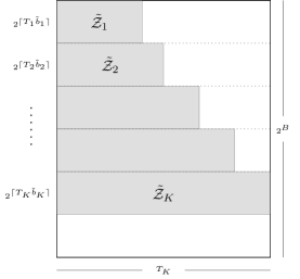
      Figure 2: An illustration of the data-dependent codebook. The big matrix represents the base code $\mathcal{Z}$, and the shaded areas are $(\widetilde{\mathcal{Z}}_{k})$, sub-matrices of size $T_{k}\times 2^{\lceil T_{k}\widetilde{b}_{k}\rceil}$ with rows normalized.

3. Transmission. Transmit or store $(\check{S}_{k})_{k=1}^{K}$ and $(\check{Z}_{(k)})_{k=1}^{K}$ by their corresponding indices.

4. Decoding & Estimation.

   1. Recover $(\check{S}_{k})$ based on the transmitted or stored indices and the common codebook $(\mathcal{S}_{k})$.

   2. Solve (4.2) and get $(\widetilde{b}_{k})$. Reconstruct $(\widetilde{\mathcal{Z}}_{k})$ using $\mathcal{Z}$ and $(\widetilde{b}_{k})$.

   3. Recover $(\check{Z}_{(k)})$ based on the transmitted or stored indices and the reconstructed codebook $(\widetilde{\mathcal{Z}}_{k})$.

   4. Estimate $\theta_{(k)}$ by

      $$\check{\theta}_{(k)}=\frac{\check{S}_{k}^{2}-T_{k}\varepsilon^{2}}{\check{S}_{k}}\sqrt{1-2^{-2\widetilde{b}_{k}}}\cdot\check{Z}_{(k)}.$$

   5. Estimate the entire vector $\theta$ by concatenating the $\check{\theta}_{(k)}$ vectors and padding with zeros; thus,

      $$\check{\theta}=\left(\check{\theta}_{(1)},\dots,\check{\theta}_{(K)},0,0,\dots\right).$$

The following theorem establishes the asymptotic optimality of this quantized estimator.

Theorem 4.1.

Let $\check{\theta}$ be the quantized estimator defined above.

1. If $B\varepsilon^{\frac{2}{2m+1}}\to\infty$, then

   $$\lim_{\varepsilon\to 0}\,\varepsilon^{-\frac{4m}{2m+1}}\sup_{\theta\in\Theta(m,c)}\mathbb{E}\|\theta-\check{\theta}\|^{2}=\mathsf{P}_{m,c}.$$

2. If $B\varepsilon^{\frac{2}{2m+1}}\to d$ for some constant $d$ as $\varepsilon\to 0$, then

   $$\lim_{\varepsilon\to 0}\,\varepsilon^{-\frac{4m}{2m+1}}\sup_{\theta\in\Theta(m,c)}\mathbb{E}\|\theta-\check{\theta}\|^{2}=\mathsf{P}_{m,c}+\mathsf{Q}_{d,m,c}.$$

3. If $B\varepsilon^{\frac{2}{2m+1}}\to 0$ and $B(\log(1/\varepsilon))^{-3}\to\infty$, then

   $$\lim_{\varepsilon\to 0}\,B^{2m}\sup_{\theta\in\Theta(m,c)}\mathbb{E}\|\theta-\check{\theta}\|^{2}=\frac{c^{2}m^{2m}}{\pi^{2m}}.$$

The expectations are with respect to the random quantized estimation scheme $Q$ and the distribution of the data.

We pause to make several remarks on this result before outlining the proof.

Remark 4.1.

The total number of bits used by this quantized estimation scheme is

$$\sum_{k=1}^{K}\lceil T_{k}\widetilde{b}_{k}\rceil+\sum_{k=1}^{K}\log\lceil\varepsilon^{-2}c(j_{k}\pi)^{-m}\rceil \leq\sum_{k=1}^{K}\lceil T_{k}\widetilde{b}_{k}\rceil+\sum_{k=1}^{K}\log\lceil\varepsilon^{-2}c\rceil$$

$${}\leq B+K+2K\rho_{\varepsilon}^{-1}+K\log\lceil c\rceil$$

$${}=B+O((\log(1/\varepsilon))^{3}),$$

where we use the fact that $K\lesssim\log^{2}(1/\varepsilon^{2})$ (See Lemma A.4). Therefore, as long as $B(\log(1/\varepsilon))^{-3}\to\infty$, the total number of bits used is asymptotically no more than $B$, the given communication budget.

Remark 4.2.

The quantized estimation scheme does not make essential use of the parameters of the Sobolev space, namely the smoothness $m$ and the radius $c$. The only exception is that in Step 1.1 the size of the codebook $\mathcal{S}_{k}$ depends on $m$ and $c$. However, suppose that we know a lower bound on the smoothness $m$, say $m\geq m_{0}$, and an upper bound on the radius $c$, say $c\leq c_{0}$. By replacing $m$ and $c$ by $m_{0}$ and $c_{0}$ respectively, we make the codebook independent of the parameters. We shall assume $m_{0}>1/2$, which leads to continuous functions. This modification does not, however, significantly increase the number of bits; in fact, the total number of bits is still $B+O(\rho_{\varepsilon}^{-3})$. Thus, we can easily make this quantized estimator minimax adaptive to the class of Sobolev ellipsoids $\{\Theta(m,c):m\geq m_{0},\;c\leq c_{0}\}$, as long as $B$ grows faster than $(\log(1/\varepsilon))^{3}$. More formally, we have

Corollary 4.1.

Suppose that $B_{\varepsilon}$ satisfies $B_{\varepsilon}(\log(1/\varepsilon))^{-3}\to\infty$. Let $\check{\theta}^{\prime}$ be the quantized estimator with the modification described above, which does not assume knowledge of $m$ and $c$. Then for $m\geq m_{0}$ and $c\leq c_{0}$,

$$\lim_{\varepsilon\to 0}\frac{\sup_{\theta\in\Theta(m,c)}\mathbb{E}\|\theta-\check{\theta}^{\prime}\|^{2}}{\inf_{\widehat{\theta},C(\widehat{\theta})\leq B}\sup_{\theta\in\Theta(m,c)}\mathbb{E}\|\theta-\widehat{\theta}\|^{2}}=1,$$

where the expectation in the numerator is with respect to the data and the randomized coding scheme, while the expectation in the denominator is only with respect to the data.

Remark 4.3.

When $B$ grows at a rate comparable to or slower than $(\log(1/\varepsilon))^{3}$, the lower bound is still achievable, just no longer by the quantized estimator we described above. The main reason is that when $B$ does not grow faster than $\log(1/\varepsilon)^{3}$, the block size $T_{1}=\lceil\log(1/\varepsilon)\rceil$ is too large. The blocking needs to be modified to get achievability in this case.

Remark 4.4.

In classical rate distortion [8, 12], the probabilistic method applied to a randomized coding scheme shows the existence of a code achieving the rate distortion bounds. Comparing to Theorem 3.1, we see that the expected risk, averaged over the randomness in the codebook, similarly achieves the quantized minimax lower bound. However, note that the average over the codebook is inside the supremum over the Sobolev space, implying that the code achieving the bound may vary over the ellipsoid. In other words, while the coding scheme generates a codebook that is used for different $\theta$, it is not known whether there is one code generated by this randomized scheme that is “universal,” and achieves the risk lower bound with high probability over the ellipsoid. The existence or non-existence of such “universal codes” is an interesting direction for further study.

Remark 4.5.

We have so far dealt with the periodic case, i.e., functions in the periodic Sobolev space $\widetilde{W}(m,c)$ defined in (3.1). For the Sobolev space $W(m,c)$, where the functions are not necessarily periodic, the lower bound given in Theorem 3.1 still holds, since $\widetilde{W}(m,c)$ is a subset of the larger class $W(m,c)$. To extend the achievability result to $W(m,c)$, we again need to relate $W(m,c)$ to an ellipsoid. Nussbaum [17] shows using spline theory that the non-periodic space can actually be expressed as an ellipsoid, where the length of the $j$th principal axis scales as $(\pi^{2}j)^{m}$ asymptotically. Based on this link between $W(m,c)$ and the ellipsoid, the techniques used here to show achievability apply, and since the principal axes scale as in the periodic case, the convergence rates remain the same.

Proof of Theorem 4.1

We now sketch the proof of Theorem 4.1, deferring the full details to Section A. To provide only an informal outline of the proof, we shall write $A_{1}\approx A_{2}$ as a shorthand for $A_{1}=A_{2}(1+o(1))$, and $A_{1}\lesssim A_{2}$ for $A_{1}\leq A_{2}(1+o(1))$, without specifying here what these $o(1)$ terms are.

To upper bound the risk $\mathbb{E}\|\check{\theta}-\theta\|^{2}$, we adopt the following sequence of approximations and inequalities. First, we discard the components whose index is greater than $N$ and show that

$$\mathbb{E}\|\check{\theta}-\theta\|^{2}\approx\mathbb{E}\sum_{k=1}^{K}\|\check{\theta}_{(k)}-\theta_{(k)}\|^{2}.$$

Since $$\check{S}_{k} S_{k} \check{\theta}_{(k)} \widehat{\theta}_{(k)}=\frac{S_{k}^{2}-T_{k}\varepsilon^{2}}{S_{k}}\sqrt{1-2^{-2\widetilde{b}_{(k)}}}\cdot\check{Z}_{(k)}$$ is close enough to , we can then safely replace by and obtain

$$\approx\mathbb{E}\sum_{k=1}^{K}\|\widehat{\theta}_{(k)}-\theta_{(k)}\|^{2}.$$

Writing $$\lambda_{k}=\frac{S_{k}^{2}-T_{k}\varepsilon^{2}}{S_{k}^{2}}$$, we further decompose the risk into

$$\begin{aligned} &=\mathbb{E}\sum_{k=1}^{K}\Big{(}\|\widehat{\theta}_{(k)}-\lambda_{k}Y_{(k)}\|^{2}+\|\lambda_{k}Y_{(k)}-\theta_{(k)}\|^{2}\\ &\hskip 72.26999pt+2\langle\widehat{\theta}_{(k)}-\lambda_{k}Y_{(k)},\lambda_{k}Y_{(k)}-\theta_{(k)}\rangle\Big{)}.\end{aligned}$$

Conditioning on the data $$Y$$ and taking the expectation with respect to the random codebook yields

$$\lesssim\mathbb{E}\sum_{k=1}^{K}\left(\frac{(S_{k}^{2}-T_{k}\varepsilon^{2})^{2}}{S_{k}^{2}}2^{-2\widetilde{b}_{k}}+\|\lambda_{k}Y_{(k)}-\theta_{(k)}\|^{2}\right).$$

By two oracle inequalities upper bounding the expectations with respect to the data, and the fact that $$\widetilde{b}$$ is the solution to (4.2),

$$\lesssim\min_{b\in\Pi_{\text{blk}}(B)}\sum_{k=1}^{K}\left(\frac{\|\theta_{(k)}\|^{4}}{\|\theta_{(k)}\|^{2}+T_{k}\varepsilon^{2}}2^{-2\bar{b}_{k}}+\frac{\|\theta_{(k)}\|^{2}T_{k}\varepsilon^{2}}{\|\theta_{(k)}\|^{2}+T_{k}\varepsilon^{2}}\right).$$

Showing that the blockwise constant oracles are almost as good as the monotone oracle, we get for some $$B^{\prime}\approx B$$

$$\lesssim\min_{b\in\Pi_{\text{mon}}(B^{\prime}),\ \omega\in\Omega_{\text{mon}}}\sum_{j=1}^{N}\left(\frac{\theta_{j}^{4}}{\theta_{j}^{2}+\varepsilon^{2}}2^{-2b_{j}}+(1-\omega_{j})^{2}\theta_{j}^{2}+\omega_{j}^{2}\varepsilon^{2}\right),$$

where $\Pi_{\text{blk}}(B)$, $\Pi_{\text{mon}}(B)$ are the classes of blockwise constant and monotone allocations of the bits defined in (A.8), (A.9), and $\Omega_{\text{mon}}$ is the class of monotone weights defined in (A.11). The proof is then completed by Lemma A.9 showing that the last quantity is equal to $V_{\varepsilon}(m,c,B)$.

5 Simulations

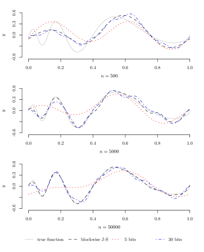
Figure 3: The damped Doppler function (solid gray) and typical realizations of the estimators under different noise levels ($n=500$, 5000, and 50000). Three estimators are used: the blockwise James-Stein estimator (dashed black), and two quantized estimator with budgets of 5 bits (dashed red) and 30 bits (dashed blue).

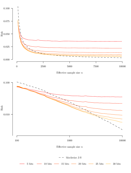
Figure 4: Risk versus effective sample size $n=1/\varepsilon^{2}$ for estimating the damped Doppler function with different estimators. The dashed line represents the risk of the blockwise James-Stein estimator, and the solid ones are for the quantized estimators with different budgets. The budgets are 5, 10, 15, 20, 25, and 30 bits, corresponding to the lines from top to bottom. The two plots are the same curves on the original scale and the log-log scale.

Here we illustrate the performance of the proposed quantized estimation scheme. We use the function

$$f(x)=\sqrt{x(1-x)}\sin\left(\frac{2.1\pi}{x+0.3}\right),\quad 0\leq x\leq 1,$$

which we shall refer to as the “damped Doppler function,” shown in Figure 3 (the gray lines). Note that the value $0.3$ differs from the value $0.05$ in the usual Doppler function used to illustrate spatial adaptation of methods such as wavelets. Since we do not address spatial adaptivity in this paper, we “slow” the oscillations of the Doppler function near zero in our illustrations.

We use this $f$ as the underlying true mean function and generate our data according to the corresponding white noise model (1.1),

$$dX(t)=f(t)dt+\varepsilon dW(t),\quad 0\leq t\leq 1.$$

We apply the blockwise James-Stein estimator, as well as the proposed quantized estimator with different communication budgets. We also vary the noise level $\varepsilon$ and, equivalently, the effective sample size $n=1/\varepsilon^{2}$.

We first show in Figure 3 some typical realizations of these estimators on data generated under different noise levels ($n=500$, 5000, and 50000 respectively). To keep the plots succinct, we show only the true function, the blockwise James-Stein estimates and quantized estimates using total bit budgets of 5 and 30 bits. We observe, in the first plot, that both quantized estimates deviate from the true function, and so does the blockwise James-Stein estimates. This is when the noise is relatively large and any quantized estimate performs poorly, no matter how large a budget is given. Both 5 bits and 30 bits appear to be “sufficient/over-sufficient” here. In the second plot, the blockwise James-Stein estimate is close to the quantized estimate with a budget of 30 bits, while with a budget of 5 bits it fails to capture the fluctuations of the true function. Thus, a budget of 30 bits is still “sufficient,” but 5 bits apparently becomes “insufficient.” In the third plot, the blockwise James-Stein estimate gives a better fit than the two quantized estimates, as both budgets become “insufficient” to achieve the optimal risk.

Next, in Figure 4 we plot the risk as a function of sample size $n$, averaging over 2000 simulations. Note that the bottom plot is the just the first plot on a log-log scale. In this set of plots, we are able to observe the phase transition for the quantized estimators. For relatively small values of $n$, all quantized estimators yield a similar error rate, with risks that are close to (or even smaller than) that of the blockwise James-Stein estimator. This is the over-sufficient regime—even the smallest budget suffices to achieve the optimal risk. As $n$ increases, the curves start to separate, with estimators having smaller bit budgets leading to worse risks compared to the blockwise James-Stein estimator, and compared to estimators with larger budgets. This can be seen as the sufficient regime for the small-budget estimators—the risks are still going down, but at a slower rate than optimal. The six quantized estimators all end up in the insufficient regime—as $n$ increases, their risks begin to flatten out, while the risk of the blockwise James-Stein estimator continues to decrease.

6 Related work and future directions

Concepts related to quantized nonparametric estimation appear in multiple communities. As mentioned in the introduction, Donoho’s 1997 Wald Lectures [9] (on the eve of the 50th anniversary of Shannon’s 1948 paper), drew sharp parallels between rate distortion, metric entropy and minimax rates, focusing on the same Sobolev function spaces we treat here. One view of the present work is that we take this correspondence further by studying how the risk continuously degrades with the level of quantization. We have analyzed the precise leading order asymptotics for quantized regression over the Sobolev spaces, showing that these rates and constants are realized with coding schemes that are adaptive to the smoothness $m$ and radius $c$ of the ellipsoid, achieving automatically the optimal rate for the regime corresponding to those parameters given the specified communication budget. Our detailed analysis is possible due to what Nussbaum [19] calls the “Pinsker phenomenon,” refering to the fact that linear filters attain the minimax rate in the over-sufficient regime. It will be interesting to study quantized nonparametric estimation in cases where the Pinsker phenomenon does not hold, for example over Besov bodies and different $L_{p}$ spaces.

Many problems of rate distortion type are similar to quantized regression. The standard “reverse water filling” construction to quantize a Gaussian source with varying noise levels plays a key role in our analysis, as shown in Section 3. In our case the Sobolev ellipsoid is an infinite Gaussian sequence model, requiring truncation of the sequence at the appropriate level depending on the targeted quantization and estimation error. In the case of Euclidean balls, Draper and Wornell [10] study rate distortion problems motivated by communication in sensor networks; this is closely related to the problem of quantized minimax estimation over Euclidean balls that we analyzed in [27]. The essential difference between rate distortion and our quantized minimax framework is that in rate distortion the quantization is carried out for a random source, while in quantized estimation we quantize our estimate of the deterministic and unknown basis coefficients. Since linear estimators are asymptotically minimax for Sobolev spaces under squared error (the “Pinsker phenomenon”), this naturally leads to an alternative view of quantizing the observations, or said differently, of compressing the data before estimation.

Statistical estimation from compressed data has appeared previously in different communities. In [26] a procedure is analyzed that compresses data by random linear transformations in the setting of sparse linear regression. Zhang and Berger [25] study estimation problems when the data are communicated from multiple sources; Ahlswede and Csiszár [2] consider testing problems under communication constraints; the use of side information is studied by Ahlswede and Burnashev [1]; other formulations in terms of multiterminal information theory are given by Han and Amari [14]; nonparametric problems are considered by Raginsky in [20]. In a distributed setting the data may be divided across different compute nodes, with distributed estimates then aggregated or pooled by communicating with a central node. The general “CEO problem” of distributed estimation was introduced by Berger, Zhang and Viswanathan [3], and has been recently studied in parametric settings in [24, 13]. These papers take the view that the data are communicated to the statistician at a certain rate, which may introduce distortion, and the goal is to study the degradation of the estimation error. In contrast, in our setting we can view the unquantized data as being fully available to the statistician at the time of estimation, with communication constraints being imposed when communicating the estimated model to a remote location.

Finally, our quantized minimax analysis shows achievability using random coding schemes, which are not computationally efficient. A natural problem is to develop practical coding schemes that come close to the quantized minimax lower bounds. In our view, the most promising approach currently is to exploit source coding schemes based on greedy sparse regression [23], applying such techniques blockwise according to the procedure we developed in Section 4.

Appendix A Proofs of Technical Results

In this section, we provide proofs for Theorems 3.1 and 4.1.

A.1 Proof of Theorem 3.1

We first show

Lemma A.1.

The quantized minimax risk is lower bounded by $V_{\varepsilon}(m,c,B_{\varepsilon})$, the value of the optimization ($\mathcal{P}_{1}$).

Proof.

As will be clear to the reader, $V_{\varepsilon}(m,c,B_{\varepsilon})$ is achieved by some $\sigma^{2}$ that is non-increasing and finitely supported. Let $\sigma^{2}$ be such that

$$\sigma_{1}^{2}\geq\dots\geq\sigma_{n}^{2}>0=\sigma_{n+1}=\dots,\ \sum_{j=1}^{n}a_{j}^{2}\sigma_{j}^{2}=\frac{c^{2}}{\pi^{2m}},$$

and let

$$\Theta_{n}(m,c)=\{\theta\in\ell_{2}:\sum_{j=1}^{n}a_{j}^{2}\theta_{j}^{2}\leq\frac{c^{2}}{\pi^{2m}},\ \theta_{j}=0\text{ for }j\geq n+1\}\subset\Theta(m,c).$$

We build on this sequence of $\sigma^{2}$ a prior distribution of $\theta$. In particular, for $\tau\in(0,1)$, write $s_{j}^{2}=(1-\tau)\sigma_{j}^{2}$ and let $\pi_{\tau}(\theta;\sigma^{2})$ be a the prior distribution on $\theta$ such that

$$\theta_{j}\sim\mathcal{N}(0,s_{j}^{2}), \quad j=1,\dots,n,$$

$$\mathbb{P}(\theta_{j}=0)=1, \quad j\geq n+1.$$

We observe that

$$R_{\varepsilon}(m,c,B_{\varepsilon}) \geq\inf_{\widehat{\theta},C(\widehat{\theta})\leq B_{\varepsilon}}\sup_{\theta\in\Theta_{n}(m,c)}\mathbb{E}\|\theta-\widehat{\theta}\|^{2}$$

$$\geq\inf_{\widehat{\theta},C(\widehat{\theta})\leq B_{\varepsilon}}\int_{\Theta_{n}(m,c)}\mathbb{E}\|\theta-\widehat{\theta}\|^{2}d\pi_{\tau}(\theta;\sigma^{2})$$

$$\geq I_{\tau}-r_{\tau}$$

where $I_{\tau}$ is the integrated risk of the optimal quantized estimator

$$I_{\tau}=\inf_{{\widehat{\theta},C(\widehat{\theta})\leq B_{\varepsilon}}}\int_{\mathbb{R}^{n}\otimes\{0\}^{\infty}}\mathbb{E}\|\theta-\widehat{\theta}\|^{2}d\pi_{\tau}(\theta;\sigma^{2})$$

and $r_{\tau}$ is the residual

$$r_{\tau}=\sup_{\widehat{\theta}\in\Theta(m,c)}\int_{\overline{\Theta(m,c)}}\mathbb{E}\|\theta-\widehat{\theta}\|^{2}d\pi_{\tau}(\theta;\sigma^{2})$$

where $\overline{\Theta(m,c)}=(\mathbb{R}^{n}\otimes\{0\}^{\infty})\backslash\Theta_{n}(m,c)$. As shown in Section 3, $\lim_{\tau\to 0}I_{\tau}$ is lower bounded by the value of the optimization

$$\min_{\mu^{2}} \ \sum_{j=1}^{\infty}\mu_{j}^{2}+\sum_{j=1}^{\infty}\frac{\sigma_{j}^{2}\varepsilon^{2}}{\sigma_{j}^{2}+\varepsilon^{2}}$$

such that $$\ \sum_{j=1}^{\infty}\frac{1}{2}\log_{+}\left(\frac{\sigma_{j}^{4}}{\mu_{j}^{2}(\sigma_{j}^{2}+\varepsilon^{2})}\right)\leq B_{\varepsilon}.$$

It then suffices to show that $r_{\tau}=o(I_{\tau})$ as $\varepsilon\to 0$ for $\tau\in(0,1)$. Let $d_{n}=\sup_{\theta\in\Theta_{n}(m,c)}\|\theta\|$, which is bounded since for any $\theta\in\Theta_{n}(m,c)$

$$\|\theta\|=\sqrt{\sum_{j}\theta_{j}^{2}}=\sqrt{\frac{1}{a_{1}^{2}}\sum_{j}a_{1}^{2}\theta_{j}^{2}}\leq\sqrt{\frac{1}{a_{1}^{2}}\sum_{j}a_{j}^{2}\theta_{j}^{2}}\leq\sqrt{\frac{1}{a_{1}^{2}}\frac{c^{2}}{\pi^{2m}}}=\frac{c}{a_{1}\pi^{m}}.$$

We have

$$r_{\tau} =\sup_{\widehat{\theta}\in\Theta(m,c)}\int_{\overline{\Theta_{n}(m,c)}}\mathbb{E}\|\theta-\widehat{\theta}\|^{2}d\pi_{\tau}(\theta;\sigma^{2})$$

$$\leq 2\int_{\overline{\Theta_{n}(m,c)}}(d_{n}^{2}+\mathbb{E}\|\theta\|^{2})d\pi_{\tau}(\theta;\sigma^{2})$$

$$\leq 2\left(d_{n}^{2}\,\mathbb{P}\left(\theta\notin{\Theta_{n}(m,c)}\right)+\left(\mathbb{P}(\theta\notin\Theta_{n}(m,c))\mathbb{E}\|\theta\|^{4}\right)^{1/2}\right)$$

where we use the Cauchy-Schwarz inequality. Noticing that

$$\mathbb{E}\|\theta\|^{4} =\mathbb{E}\bigg{(}\Big{(}\sum_{j=1}^{n}\theta_{j}^{2}\Big{)}^{2}\bigg{)}$$

$$=\sum_{j_{1}\neq j_{2}}\mathbb{E}(\theta_{j_{1}}^{2})\mathbb{E}(\theta_{j_{2}}^{2})+\sum_{j=1}^{n}\mathbb{E}(\theta_{j}^{4})$$

$$\leq\sum_{j_{1}\neq j_{2}}s_{j_{1}}^{2}s_{j_{2}}^{2}+3\sum_{j=1}^{n}s_{j}^{4}$$

$$\leq 3\Big{(}\sum_{j=1}^{n}s_{j}^{2}\Big{)}^{2}\leq 3d_{n}^{4},$$

we obtain

$$r_{\tau} \leq 2d_{n}^{2}\left(\mathbb{P}\left(\theta\notin{\Theta_{n}(m,c)}\right)+\sqrt{3\mathbb{P}\left(\theta\notin{\Theta_{n}(m,c)}\right)}\right)$$

$$\leq 6d_{n}^{2}\sqrt{\mathbb{P}\left(\theta\notin{\Theta_{n}(m,c)}\right)}.$$

Thus, we only need to show that $\sqrt{\mathbb{P}\left(\theta\notin{\Theta_{n}(m,c)}\right)}=o(I_{\tau})$. In fact,

$$\mathbb{P}(\theta\notin \Theta_{n}(m,c))$$

$$=\mathbb{P}\left(\sum_{j=1}^{n}a_{j}^{2}\theta_{j}^{2}>\frac{c^{2}}{\pi^{2m}}\right)$$

$$=\mathbb{P}\left(\sum_{j=1}^{n}a_{j}^{2}(\theta_{j}^{2}-\mathbb{E}(\theta_{j}^{2}))>\frac{c^{2}}{\pi^{2m}}-(1-\tau)\sum_{j=1}^{n}a_{j}^{2}\sigma_{j}^{2}\right)$$

$$=\mathbb{P}\left(\sum_{j=1}^{n}a_{j}^{2}(\theta_{j}^{2}-\mathbb{E}(\theta_{j}^{2}))>\frac{\tau c^{2}}{\pi^{2m}}\right)$$

$$=\mathbb{P}\left(\sum_{j=1}^{n}a_{j}^{2}s_{j}^{2}(Z_{j}^{2}-1)>\frac{\tau}{1-\tau}\sum_{j=1}^{n}a_{j}^{2}s_{j}^{2}\right)$$

where $Z_{j}\sim\mathcal{N}(0,1)$. By Lemma A.2, we get

$$\mathbb{P}(\theta\notin\Theta_{n}(m,c))\leq\exp\left(-\frac{\tau^{2}}{8(1-\tau)^{2}}\frac{\sum_{j=1}^{n}a_{j}^{2}s_{j}^{2}}{\max_{1\leq j\leq n}a_{j}^{2}s_{j}^{2}}\right)=\exp\left(-\frac{\tau^{2}}{8(1-\tau)^{2}}\frac{\sum_{j=1}^{n}a_{j}^{2}\sigma_{j}^{2}}{\max_{1\leq j\leq n}a_{j}^{2}\sigma_{j}^{2}}\right)$$

Next we will show that for the $\sigma^{2}$ that achieves $V_{\varepsilon}(m,c,B_{\varepsilon})$, we have $\sqrt{\mathbb{P}(\theta\notin\Theta_{n}(m,c))}=o(I_{\tau})$. For the sufficient regime where $B_{\varepsilon}\varepsilon^{\frac{2}{2m+1}}\to\infty$ as $\varepsilon\to 0$, it is shown in [22] that $\max_{1\leq j\leq n}a_{j}^{2}\sigma_{j}^{2}=O(\varepsilon^{\frac{2}{2m+1}})$ and $I_{\tau}=O(\varepsilon^{\frac{4m}{2m+1}})$, and hence that $\sqrt{\mathbb{P}(\theta\notin\Theta_{n}(m,c))}=o(I_{\tau})$. For the insufficient regime where $B_{\varepsilon}\varepsilon^{\frac{2}{2m+1}}\to 0$ but still $B_{\varepsilon}\to\infty$ as $\varepsilon\to 0$, an achieving sequence $\sigma^{2}$ is given later by (A.4) and (A.3). We obtain that $\max_{1\leq j\leq n}a_{j}^{2}\sigma_{j}^{2}=O(B_{\varepsilon}^{-1})$ and $I_{\tau}=O(B_{\varepsilon}^{-2m})$, and therefore $\sqrt{\mathbb{P}(\theta\notin\Theta_{n}(m,c))}=o(I_{\tau})$. The sufficient regime where $B_{\varepsilon}\varepsilon^{\frac{2}{2m+1}}\to d$ for some constant $d$ is a bit more complicated as we don’t have an explicit formula for the optimal sequence $\sigma^{2}$. However, by Lemma 3.3, for the continuous approximation $\sigma^{2}(x)$ such that $\sigma^{2}_{j}=\sigma^{2}(jh)h^{2m+1}$, we have

$$\lambda x^{2m}\sigma^{2}(x) =\frac{\sigma^{2}(x)}{(\sigma^{2}(x)+1)^{2}}+\alpha\cdot\frac{\sigma^{2}(x)+2}{\sigma^{2}(x)+1}\leq\frac{1}{4}+2\alpha$$

where $\alpha=\exp\left(\frac{1}{x_{0}}\int_{0}^{x_{0}}\log\frac{\sigma^{4}(x)}{\sigma^{2}(x)+1}dx-\frac{2d}{x_{0}}\right)$ and $\lambda$ are both constants. Therefore,

$$\max_{1\leq j\leq n}a_{j}^{2}\sigma_{j}^{2}\approx j^{2m}\sigma^{2}(jh)h^{2m+1}\leq\frac{1}{\lambda}(\frac{1}{4}+2\alpha)\cdot h.$$

Note that $\sum_{j=1}^{n}a_{j}^{2}\sigma^{2}_{j}=O(h^{2m})$ and that $h=\varepsilon^{\frac{2}{2m+1}}$. We obtain that for this case $I_{\tau}=O(\varepsilon^{\frac{4m}{2m+1}})$ and $\sqrt{\mathbb{P}(\theta\notin\Theta_{n}(m,c))}=o(I_{\tau})$. Thus, for each of the three regimes, we have $r_{\tau}=o(I_{\tau})$. ∎

Lemma A.2 (Lemma 3.5 in [22]).

Suppose that $X_{1},\dots,X_{n}$ are i.i.d. $\mathcal{N}(0,1)$. For $t\in(0,1)$ and $\omega_{j}>0$, $j=1,\dots,n$, we have

$$\mathbb{P}\left(\sum_{j=1}^{n}\omega_{j}(X_{j}^{2}-1)>t\sum_{j=1}^{n}X_{j}\right)\leq\exp\left(-\frac{t^{2}\sum_{j=1}^{n}\omega_{j}}{8\max_{1\leq j\leq n}\omega_{j}}\right).$$

Proof of Lemma 3.1.

This is in fact Pinsker’s theorem, which gives the exact asymptotic minimax risk of estimation of normal means in the Sobolev ellipsoid. The proof can be found in [19] and [22]. ∎

Proof of Lemma 3.2.

As argued in Section 3 for the lower bound in the sufficient regime, optimization problem ($\mathcal{Q}_{1}$) can be reformulated as

$$\max_{\sigma^{2},J} \ J\eta \mathcal{Q}_{2}$$ ()

such that $$\ \frac{1}{2}\sum_{j=1}^{J}\log_{+}\left(\frac{\sigma_{j}^{4}}{\eta(\sigma_{j}^{2}+\varepsilon^{2})}\right)\leq B_{\varepsilon}$$

$$\ \sum_{j=1}^{J}a_{j}^{2}\sigma_{j}^{2}\leq\frac{c^{2}}{\pi^{2m}}$$

$$\ (\sigma_{j}^{2})\text{ is decreasing and }\frac{\sigma_{J}^{4}}{\sigma_{J}^{2}+\varepsilon^{2}}\geq\eta.$$

Now suppose that we have a series ($\sigma_{j}^{2}$) which satisfies the last constraint and is supported on $\{1,\dots,J\}$. By the first constraint, we have that

$$J\eta =J\exp\left(-\frac{2B_{\varepsilon}}{J}\right)\left(\prod_{j=1}^{J}\frac{\sigma_{j}^{4}}{\sigma_{j}^{2}+\varepsilon^{2}}\right)^{\frac{1}{J}}$$

$$\leq J\exp\left(-\frac{2B_{\varepsilon}}{J}\right)\left(\prod_{j=1}^{J}\sigma_{j}^{2}\right)^{\frac{1}{J}}$$

$$=J\exp\left(-\frac{2B_{\varepsilon}}{J}\right)\left(\prod_{j=1}^{J}a_{j}^{2}\sigma_{j}^{2}\right)^{\frac{1}{J}}\left(\prod_{j=1}^{J}a_{j}^{-2}\right)^{\frac{1}{J}}$$

$$\leq\exp\left(-\frac{2B_{\varepsilon}}{J}\right)\left(\sum_{j=1}^{J}a_{j}^{2}\sigma_{j}^{2}\right)\left(\prod_{j=1}^{J}a_{j}^{-2}\right)^{\frac{1}{J}}$$

$$\leq\frac{c^{2}}{\pi^{2m}}\exp\left(-\frac{2B_{\varepsilon}}{J}\right)\left(\prod_{j=1}^{J}a_{j}^{-2}\right)^{\frac{1}{J}}$$

$$=\frac{c^{2}}{\pi^{2m}}\left(\exp\left(\frac{B_{\varepsilon}}{m}\right)J!\right)^{-\frac{2m}{J}}.$$ (A.1)

This provides a series of upper bounds for $Q_{\varepsilon}(m,c,B_{\varepsilon})$ parameterized by $J$. To minimize (A.1) over $J$, we look at the ratio of the neighboring terms with $J$ and $J+1$, and compare it to 1. We obtain that the optimal $J$ satisfies

$$\frac{J^{J}}{J!}<\exp\left(\frac{B_{\varepsilon}}{m}\right)\leq\frac{(J+1)^{J+1}}{(J+1)!}.$$ (A.2)

Denote this optimal $J$ by $J_{\varepsilon}$. By Stirling’s approximation, we have

$$\lim_{\varepsilon\to 0}\frac{B_{\varepsilon}/m}{J_{\varepsilon}}=1,$$ (A.3)

and plugging this asymptote into (A.1), we get as $\varepsilon\to 0$

$$\frac{c^{2}}{\pi^{2m}}\left(\exp\left(\frac{B_{\varepsilon}}{m}\right)J_{\varepsilon}!\right)^{-\frac{2m}{J_{\varepsilon}}}\sim\frac{c^{2}}{\pi^{2m}}J_{\varepsilon}^{-2m}\sim\frac{c^{2}m^{2m}}{\pi^{2m}}B_{\varepsilon}^{-2m}.$$

This gives the desired upper bound (3.6).

Next we show that the upper bound (3.6) is asymptotically achievable when $B_{\varepsilon}\varepsilon^{\frac{2}{2m+1}}\to 0$ and $B_{\varepsilon}\to\infty$. It suffices to find a feasible solution that attains (3.6). Let

$$\widetilde{\sigma}^{2}_{j}=\frac{c^{2}/\pi^{2m}}{J_{\varepsilon}a_{j}^{2}},\ j=1,\dots,J_{\varepsilon}.$$ (A.4)

Note that the entire sequence of $(\widetilde{\sigma}^{2}_{j})_{j=1}^{J_{\varepsilon}}$ does not qualify for a feasible solution, since the first constraint in ($\mathcal{Q}_{2}$) won’t be satisfied for any $\eta\leq\frac{\widetilde{\sigma}_{J_{\varepsilon}}^{4}}{\widetilde{\sigma}_{J_{\varepsilon}}^{2}+\varepsilon^{2}}$. We keep only the first $J_{\varepsilon}^{\prime}$ terms of $(\widetilde{\sigma}^{2}_{j})$, where $J_{\varepsilon}^{\prime}$ is the largest $j$ such that

$$\frac{\widetilde{\sigma}^{4}_{j}}{\widetilde{\sigma}^{2}_{j}+\varepsilon^{2}}\geq\widetilde{\sigma}^{2}_{J_{\varepsilon}}.$$ (A.5)

Thus,

$$\sum_{j=1}^{J_{\varepsilon}^{\prime}}\frac{1}{2}\log_{+}\left(\frac{\frac{\widetilde{\sigma}^{4}_{j}}{\widetilde{\sigma}_{j}^{2}+\varepsilon^{2}}}{\widetilde{\sigma}_{J_{\varepsilon}}^{2}}\right)\leq\sum_{j=1}^{J_{\varepsilon}^{\prime}}\frac{1}{2}\log_{+}\left(\frac{\widetilde{\sigma}_{j}^{2}}{\widetilde{\sigma}_{J_{\varepsilon}}^{2}}\right)\leq\sum_{j=1}^{J_{\varepsilon}}\frac{1}{2}\log_{+}\left(\frac{\widetilde{\sigma}_{j}^{2}}{\widetilde{\sigma}_{J_{\varepsilon}}^{2}}\right)\leq B_{\varepsilon},$$

where the last inequality is due to (A.2). This tells us that setting $\eta=\widetilde{\sigma}_{J_{\varepsilon}}^{2}$ leads to a feasible solution to ($\mathcal{Q}_{2}$). As a result,

$$Q_{\varepsilon}(m,c,B_{\varepsilon})\geq J^{\prime}_{\varepsilon}\widetilde{\sigma}^{2}_{J_{\varepsilon}}.$$ (A.6)

If we can show that $J_{\varepsilon}^{\prime}\sim J_{\varepsilon}$, then

$$J^{\prime}_{\varepsilon}\widetilde{\sigma}^{2}_{J_{\varepsilon}}\sim J_{\varepsilon}\widetilde{\sigma}^{2}_{J_{\varepsilon}}\sim\frac{c^{2}m^{2m}}{\pi^{2m}}B_{\varepsilon}^{-2m}.$$ (A.7)

To show that $J_{\varepsilon}^{\prime}\sim J_{\varepsilon}$, it suffices to show that $a_{J_{\varepsilon}^{\prime}}\sim a_{J_{\varepsilon}}$. Plugging the formula of $\widetilde{\sigma}^{2}_{j}$ into (A.5) and solving for $a^{2}_{J_{\varepsilon}^{\prime}}$, we get

$$a^{2}_{J_{\varepsilon}^{\prime}} \sim\frac{\displaystyle-\frac{c^{2}}{\pi^{2m}J_{\varepsilon}}+\sqrt{(\frac{c^{2}}{\pi^{2m}J_{\varepsilon}})^{2}+4\frac{c^{2}}{\pi^{2m}J_{\varepsilon}}\varepsilon^{2}a_{J_{\varepsilon}}^{2}}}{2\varepsilon^{2}}$$

$$\sim\frac{\displaystyle-\frac{c^{2}}{\pi^{2m}J_{\varepsilon}}+\frac{c^{2}}{\pi^{2m}J_{\varepsilon}}+\frac{1}{2}\frac{\pi^{2m}J_{\varepsilon}}{c^{2}}4\frac{c^{2}}{\pi^{2m}J_{\varepsilon}}\varepsilon^{2}a_{J_{\varepsilon}}^{2}}{2\varepsilon^{2}}=a_{J_{\varepsilon}}^{2}$$

where the equivalence is due to the assumption $B_{\varepsilon}\varepsilon^{\frac{2}{2m+1}}\to 0$ and a Taylor’s expansion of the function $\sqrt{x}$. ∎

Proof of Lemma 3.3.

Suppose that $\sigma^{2}(x)$ with $x_{0}$ solves ($\mathcal{P}_{4}$). Consider function $\sigma^{2}(x)+\xi v(x)$ such that it is still feasible for ($\mathcal{P}_{4}$), and thus we have

$$\int_{0}^{x_{0}}x^{2m}v(x)dx\leq 0.$$

Now plugging $\sigma^{2}(x)+\xi v(x)$ for $\sigma^{2}(x)$ in the objective function of ($\mathcal{P}_{4}$), taking derivative with respect to $\xi$, and letting $\xi\to 0$, we must have

$$\int_{0}^{x_{0}}\frac{v(x)}{(\sigma^{2}(x)+1)^{2}}dx+x_{0}\exp\left(\frac{1}{x_{0}}\int_{0}^{x_{0}}\log\frac{\sigma^{4}(x)}{\sigma^{2}(x)+1}dx-\frac{2d}{x_{0}}\right)\frac{1}{x_{0}}\int_{0}^{x_{0}}\frac{2v(x)}{\sigma^{2}(x)}-\frac{v(x)}{\sigma^{2}(x)+1}dx\leq 0,$$

which, after some calculation and rearrangement of terms, yields

$$\int_{0}^{x_{0}}v(x)\left(\frac{1}{(\sigma^{2}(x)+1)^{2}}+\exp\left(\frac{1}{x_{0}}\int_{0}^{x_{0}}\log\frac{\sigma^{4}(x)}{\sigma^{2}(x)+1}dx-\frac{2d}{x_{0}}\right)\frac{\sigma^{2}(x)+2}{\sigma^{2}(x)(\sigma^{2}(x)+1)}\right)dx\leq 0.$$

Thus, by the lemma that follows, we obtain that for some $\lambda$

$$\frac{1}{(\sigma^{2}(x)+1)^{2}}+\exp\left(\frac{1}{x_{0}}\int_{0}^{x_{0}}\log\frac{\sigma^{4}(y)}{\sigma^{2}(y)+1}dy-\frac{2d}{x_{0}}\right)\frac{\sigma^{2}(x)+2}{\sigma^{2}(x)(\sigma^{2}(x)+1)}=\lambda x^{2m}.$$

∎

Lemma A.3.

Suppose that $f(x)$ and $g(x)$ are two non-zero functions on $(0,x_{0})$ such that for any $v(x)$ satisfying $\int_{0}^{x_{0}}f(x)v(x)dx\leq 0$, it holds that $\int_{0}^{x_{0}}g(x)v(x)dx\leq 0$. Then there exists a constant $\lambda$ such that $f(x)=\lambda g(x)$.

Proof.

First we show that for any $v(x)$ such that $\int_{0}^{x_{0}}f(x)v(x)dx=0$ we must have $\int_{0}^{x_{0}}g(x)v(x)dx=0$. Otherwise, suppose that $v_{0}(x)$ is such that $\int_{0}^{x_{0}}f(x)v_{0}(x)dx=0$ and $\int_{0}^{x_{0}}g(x)v_{0}(x)dx<0$. Then take another $v(x)$ with $\int_{0}^{x_{0}}f(x)v(x)dx\leq 0$ and consider $v_{\gamma}(x)=v(x)-\gamma v_{0}(x)$. We have $\int_{0}^{x_{0}}f(x)v_{\gamma}(x)dx\leq 0$ and $\int_{0}^{x_{0}}g(x)v_{\gamma}(x)=\int_{0}^{x_{0}}v(x)g(x)dx-\gamma\int_{0}^{x_{0}}g(x)v_{0}(x)dx>0$ for large enough $\gamma$, which results in contradiction.

Let $\lambda=\int_{0}^{x_{0}}f(x)^{2}dx/\int_{0}^{x_{0}}f(x)g(x)dx$ as the denominator cannot be zero. In fact, if $\int_{0}^{x_{0}}f(x)g(x)dx=0$, it would imply that $\int_{0}^{x_{0}}g(x)^{2}dx=0$ and hence $g(x)\equiv 0$. Now consider the function $f(x)-\lambda g(x)$. Notice that we have $\int_{0}^{x_{0}}f(x)(f(x)-\lambda g(x))dx=0$ by the definition of $\lambda$. It follows that $\int_{0}^{x_{0}}g(x)(f(x)-\lambda g(x))dx=0$, and therefore, $\int_{0}^{x_{0}}(f(x)-\lambda g(x))^{2}dx=0$, which concludes the proof. ∎

A.2 Proof of Theorem 4.1

Now we give the details of the proof of Theorem 4.1. For the purpose of our analysis, we define two allocations of bits, the monotone allocation and the blockwise constant allocation,

$$\Pi_{\text{blk}}(B) =\left\{(b_{j})_{j=1}^{\infty}:\ \sum_{j=1}^{\infty}b_{j}\leq B,\ b_{j}=\bar{b}_{k}\text{ for }j\in J_{k},\ 0\leq b_{j}\leq b_{\max}\right\},$$ (A.8)

$$\Pi_{\text{mon}}(B) =\left\{(b_{j})_{j=1}^{\infty}:\ \sum_{j=1}^{\infty}b_{j}\leq B,\ b_{j-1}\geq b_{j},\ 0\leq b_{j}\leq b_{\max}\right\},$$ (A.9)

where $b_{\max}=2\log(1/\varepsilon)$. We also define two classes of weights, the monotonic weights and the blockwise constant weights,

$$\Omega_{\text{blk}} =\left\{(\omega_{j})_{j=1}^{\infty}:\ \omega_{j}=\bar{\omega}_{k}\text{ for }j\in J_{k},\ 0\leq\omega_{j}\leq 1\right\},$$ (A.10)

$$\Omega_{\text{mon}} =\left\{(\omega_{j})_{j=1}^{\infty}:\ \omega_{j-1}\geq\omega_{j},\ 0\leq\omega_{j}\leq 1\right\}.$$ (A.11)

We will also need the following results from [22] regarding the weakly geometric system of blocks.

Lemma A.4.

Let $\{J_{k}\}$ be a weakly geometric block system defined by (4.1). Then there exists $0<\varepsilon_{0}<1$ and $C>0$ such that for any $\varepsilon\in(0,\varepsilon_{0})$,

$$K\leq C\log^{2}(1/\varepsilon),$$

$$\max_{1\leq k\leq K-1}\frac{T_{k+1}}{T_{k}}\leq 1+3\rho_{\varepsilon}.$$

We divide the proof into four steps.

Step 1. Truncation and replacement

The loss of the quantized estimator $\check{\theta}$ can be decomposed into

$$\|\check{\theta}-\theta\|^{2}=\sum_{k=1}^{K}\|\check{\theta}_{(k)}-\theta_{(k)}\|^{2}+\sum_{j=N+1}^{\infty}\theta_{j}^{2},$$

where the remainder term satisfies

$$\sum_{j=N+1}^{\infty}\theta_{j}^{2}\leq N^{-2m}\sum_{j=N+1}^{\infty}a_{j}^{2}\theta_{j}^{2}=O(N^{-2m}).$$

If we assume that $m>1/2$, which corresponds to classes of continuous functions, the remainder term is then $o(\varepsilon^{2})$. If $m\leq 1/2$, the remainder term is on the order of $O(\varepsilon^{4m})$, which is still negligible compared to the order of the lower bound $\varepsilon^{\frac{4m}{2m+1}}$. To ease the notation, we will assume that $m>1/2$, and write the remainder term as $o(\varepsilon^{2})$, but need to bear in mind that the proof works for all $m>0$. We can thus discard the remainder term in our analysis. Recall that the quantized estimate for each block is given by

$$\check{\theta}_{(k)}=\frac{\check{S}_{k}^{2}-T_{k}\varepsilon^{2}}{\check{S}_{k}}\sqrt{1-2^{-2\widetilde{b}_{k}}}\check{Z}_{(k)},$$

and consider the following estimate with $\check{S}_{k}$ replaced by $S_{k}$

$$\widehat{\theta}_{(k)}=\frac{S_{k}^{2}-T_{k}\varepsilon^{2}}{S_{k}}\sqrt{1-2^{-2\widetilde{b}_{k}}}\check{Z}_{(k)}.$$

Notice that

$$\|\widehat{\theta}_{(k)}-\check{\theta}_{(k)}\| =\left|\frac{\check{S}_{k}^{2}-T_{k}\varepsilon^{2}}{\check{S}_{k}}-\frac{S_{k}^{2}-T_{k}\varepsilon^{2}}{S_{k}}\right|\sqrt{1-2^{-2\widetilde{b}_{k}}}\|\check{Z}_{(k)}\|$$

$$\leq\left|\frac{\check{S}_{k}S_{k}+T_{k}\varepsilon^{2}}{\check{S}_{k}S_{k}}\right|\left|\check{S}_{k}-S_{k}\right|$$

$$\leq 2\varepsilon^{2}$$

where the last inequality is because $\check{S}_{k}S_{k}\geq T_{k}\varepsilon^{2}$ and $\left|\check{S}_{k}-S_{k}\right|\leq\varepsilon^{2}$. Thus we can safely replace $\check{\theta}_{(k)}$ by $\widehat{\theta}_{(k)}$ because

$$\|\check{\theta}_{(k)} -\theta_{(k)}\|^{2}$$

$$=\|\check{\theta}_{(k)}-\widehat{\theta}_{(k)}+\widehat{\theta}_{(k)}-\theta_{(k)}\|^{2}$$

$$\leq\|\check{\theta}_{(k)}-\widehat{\theta}_{(k)}\|^{2}+\|\widehat{\theta}_{(k)}-\theta_{(k)}\|^{2}+2\|\check{\theta}_{(k)}-\widehat{\theta}_{(k)}\|\|\widehat{\theta}_{(k)}-\theta_{(k)}\|$$

$$=\|\widehat{\theta}_{(k)}-\theta_{(k)}\|^{2}+O(\varepsilon^{2}).$$

Therefore, we have

$$\mathbb{E}\|\check{\theta}-\theta\|^{2}=\mathbb{E}\sum_{k=1}^{K}\|\widehat{\theta}_{(k)}-\theta_{(k)}\|^{2}+O(K\varepsilon^{2}).$$

Step 2. Expectation over codebooks

Now conditioning on the data $Y$, we work under the probability measure introduced by the random codebook. Write

$$\lambda_{k}=\frac{S_{k}^{2}-T_{k}\varepsilon^{2}}{S_{k}^{2}}\text{ and }Z_{(k)}=\frac{Y_{(k)}}{\|Y_{(k)}\|}.$$

We decompose and examine the following term

$$A_{k} =\|\widehat{\theta}_{(k)}-\theta_{(k)}\|^{2}$$

$$=\|\widehat{\theta}_{(k)}-\lambda_{k}S_{k}Z_{(k)}+\lambda_{k}S_{k}Z_{(k)}-\theta_{(k)}\|^{2}$$

$$=\underbrace{\|\widehat{\theta}_{(k)}-\lambda_{k}S_{k}Z_{(k)}\|^{2}}_{A_{k,1}}+\underbrace{\|\lambda_{k}S_{k}Z_{(k)}-\theta_{(k)}\|^{2}}_{A_{k,2}}$$

$$\hskip 72.26999pt+\underbrace{2\langle\widehat{\theta}_{(k)}-\lambda_{k}S_{k}Z_{(k)},\lambda_{k}S_{k}Z_{(k)}-\theta_{(k)}\rangle}_{A_{k,3}}.$$

To bound the expectation of the first term $A_{k,1}$, we need the following lemma, which bounds the probability of the distortion of a codeword exceeding the desired value.

Lemma A.5.

Suppose that $Z_{1},\dots,Z_{n}$ are independent and each follows the uniform distribution on the $t$-dimensional unit sphere $\mathbb{S}^{t-1}$. Let $y\in\mathbb{S}^{t-1}$ be a fixed vector, and

$$Z^{*}=\operatorname*{\arg\min}_{z\in Z_{1:n}}\left\|\sqrt{1-2^{-2q}}z-y\right\|^{2}.$$

If $n=2^{qt}$, then

$$\mathbb{E}\left\|\sqrt{1-2^{-2q}}Z^{*}-y\right\|^{2}\leq 2^{-2q}\left(1+\nu(t)\right)+2e^{-2t}$$

where

$$\nu(t)=\frac{6\log t+7}{t-6\log t-7}.$$

Observe that

$$A_{k,1} =\left\|\widehat{\theta}_{(k)}-\lambda_{k}S_{k}Z_{(k)}\right\|^{2}$$

$$=\left\|\lambda_{k}S_{k}\sqrt{1-2^{-2\widetilde{b}_{k}}}\check{Z}_{(k)}-\lambda_{k}S_{k}Z_{(k)}\right\|^{2}$$

$$=\lambda_{k}^{2}S_{k}^{2}\left\|\sqrt{1-2^{-2\widetilde{b}_{k}}}\check{Z}_{(k)}-Z_{(k)}\right\|^{2}.$$

Then, it follows as a result of Lemma A.5 that

$$\mathbb{E}\left(A_{k,1}\,|\,Y_{(k)}\right) \leq\frac{(S_{k}^{2}-T_{k}\varepsilon^{2})^{2}}{S_{k}^{2}}\left(2^{-2\widetilde{b}_{k}}(1+\nu_{\varepsilon})+2e^{-2T_{k}}\right)$$

$$\leq\frac{(S_{k}^{2}-T_{k}\varepsilon^{2})^{2}}{S_{k}^{2}}\left(2^{-2\widetilde{b}_{k}}(1+\nu_{\varepsilon})+2e^{-2T_{1}}\right)$$

$$\leq\frac{(S_{k}^{2}-T_{k}\varepsilon^{2})^{2}}{S_{k}^{2}}2^{-2\widetilde{b}_{k}}(1+\nu_{\varepsilon})+\frac{2c^{2}}{(j_{k}\pi)^{2m}}\varepsilon^{2},$$

where $\nu_{\varepsilon}=\frac{6\log T_{1}+7}{T_{1}-6\log T_{1}-7}$. Since $A_{k,2}$ only depends on $Y_{(k)}$, $\mathbb{E}\left(A_{k,2}\,|\,Y_{(k)}\right)=A_{k,2}$. Next we consider the cross term $A_{k,3}$. Write $\gamma_{k}=\frac{\langle\theta_{(k)},Y_{(k)}\rangle}{\|Y_{(k)}\|^{2}}$ and

$$A_{k,3} =2\left\langle\widehat{\theta}_{(k)}-\lambda_{k}S_{k}Z_{(k)},\lambda_{k}S_{k}Z_{(k)}-\theta_{(k)}\right\rangle$$

$$=\underbrace{2\left\langle\widehat{\theta}_{(k)}-\lambda_{k}S_{k}Z_{(k)},\gamma_{k}Y_{(k)}-\theta_{(k)}\right\rangle}_{A_{k,3a}}$$

$$\hskip 72.26999pt+\underbrace{2\left\langle\widehat{\theta}_{(k)}-\lambda_{k}S_{k}Z_{(k)},\lambda_{k}S_{k}Z_{(k)}-\gamma_{k}Y_{(k)}\right\rangle}_{A_{k,3b}}.$$

The quantity $\gamma_{k}$ is chosen such that $\langle Y_{(k)},\gamma_{k}Y_{(k)}-\theta_{(k)}\rangle=0$ and therefore

$$A_{k,3a} =2\left\langle\widehat{\theta}_{(k)}-\lambda_{k}S_{k}Z_{(k)},\gamma_{k}Y_{(k)}-\theta_{(k)}\right\rangle$$

$$=2\left\langle\Pi_{Y_{(k)}^{\perp}}(\widehat{\theta}_{(k)}-\lambda_{k}S_{k}Z_{(k)}),\gamma_{k}Y_{(k)}-\theta_{(k)}\right\rangle$$

where $\Pi_{Y_{(k)}^{\perp}}$ denotes the projection onto the orthogonal complement of $Y_{(k)}$. Due to the choice of $\check{Z}_{(k)}$, the projection $\Pi_{Y_{(k)}^{\perp}}(\widehat{\theta}_{(k)}-\lambda_{k}S_{k}Z_{(k)})$ is rotation symmetric and hence $\mathbb{E}\left(A_{k,3a}\,|\,Y_{(k)}\right)=0$. Finally, for $A_{k,3b}$ we have

$$\mathbb{E}\left(A_{k,3b}\,|\,Y_{(k)}\right)$$

$$\leq 2\|\lambda_{k}S_{k}Z_{(k)}-\gamma_{k}Y_{(k)}\|\mathbb{E}\left(\|\widehat{\theta}_{(k)}-\lambda_{k}S_{k}Z_{(k)}\|\,|\,Y_{(k)}\right)$$

$$\leq 2\|\lambda_{k}S_{k}Z_{(k)}-\gamma_{k}Y_{(k)}\|\sqrt{\mathbb{E}\left(\|\widehat{\theta}_{(k)}-\lambda_{k}S_{k}Z_{(k)}\|^{2}\,|\,Y_{(k)}\right)}$$

$$\leq 2\|\lambda_{k}S_{k}Z_{(k)}-\gamma_{k}Y_{(k)}\|\sqrt{\frac{(S_{k}^{2}-T_{k}\varepsilon^{2})^{2}}{S_{k}^{2}}2^{-2\widetilde{b}_{k}}(1+\nu_{\varepsilon})+\frac{2c^{2}}{(j_{k}\pi)^{2m}}\varepsilon^{2}}.$$

Combining all the analyses above, we have

$$\mathbb{E}\left(A_{k}\,|\,Y_{(k)}\right)$$

$$\leq\frac{(S_{k}^{2}-T_{k}\varepsilon^{2})^{2}}{S_{k}^{2}}2^{-2\widetilde{b}_{k}}(1+\nu_{\varepsilon})+\frac{2c^{2}}{(j_{k}\pi)^{2m}}\varepsilon^{2}+\|\lambda_{k}S_{k}Z_{(k)}-\theta_{(k)}\|^{2}$$

$$\hskip 14.45377pt+2\|\lambda_{k}S_{k}Z_{(k)}-\gamma_{k}Y_{(k)}\|\sqrt{\frac{(S_{k}^{2}-T_{k}\varepsilon^{2})^{2}}{S_{k}^{2}}2^{-2\widetilde{b}_{k}}(1+\nu_{\varepsilon})+\frac{2c^{2}}{(j_{k}\pi)^{2m}}\varepsilon^{2}},$$

and summing over $k$ we get

$$\mathbb{E}\left(\|\check{\theta}-\theta\|^{2}\,|\,Y\right)$$ (A.12)

$$\leq\sum_{k=1}^{K}\frac{(S_{k}^{2}-T_{k}\varepsilon^{2})^{2}}{S_{k}^{2}}2^{-2\widetilde{b}_{k}}(1+\nu_{\varepsilon})+\sum_{k=1}^{K}\|\lambda_{k}S_{k}Z_{(k)}-\theta_{(k)}\|^{2}$$

$$\hskip 14.45377pt+2\sum_{k=1}^{K}\|\lambda_{k}S_{k}Z_{(k)}-\gamma_{k}Y_{(k)}\|\sqrt{\frac{(S_{k}^{2}-T_{k}\varepsilon^{2})^{2}}{S_{k}^{2}}2^{-2\widetilde{b}_{k}}(1+\nu_{\varepsilon})+O(\varepsilon^{2})}+O(K\varepsilon^{2}).$$

Step 3. Expectation over data

First we will state three lemmas, which bound the deviation of the expectation of some particular functions of the norm of a Gaussian vector to the desired quantities. The proofs are given in Section A.3.

Lemma A.6.

Suppose that $X_{i}\sim\mathcal{N}(\theta_{i},\sigma^{2})$ independently for $i=1,\dots,n$, where $\|\theta\|^{2}\leq c^{2}$. Let $S$ be given by

$$S=\begin{cases}\sqrt{n\sigma^{2}}&\text{if }\|X\|<\sqrt{n\sigma^{2}}\\ \sqrt{n\sigma^{2}}+c&\text{if }\|X\|>\sqrt{n\sigma^{2}}+c\\ \|X\|&\text{otherwise}.\end{cases}$$

Then there exists some absolute constant $C_{0}$ such that

$$\mathbb{E}\left(\frac{S^{2}-n\sigma^{2}}{S}-\frac{\langle\theta,X\rangle}{\|X\|}\right)^{2}\leq C_{0}\sigma^{2}.$$

Lemma A.7.

Let $X$ and $S$ be the same as defined in Lemma A.6. Then for $n>4$

$$\mathbb{E}\frac{(S^{2}-n\sigma^{2})^{2}}{S^{2}}\leq\frac{\|\theta\|^{4}}{\|\theta\|^{2}+n\sigma^{2}}+\frac{4n}{n-4}\sigma^{2}.$$

Lemma A.8.

Let $X$ and $S$ be the same as defined in Lemma A.6. Define

$$\widehat{\theta}_{+}=\left(\frac{\|X\|^{2}-n\sigma^{2}}{\|X\|^{2}}\right)_{+}X,\quad\widehat{\theta}_{\dagger}=\frac{S^{2}-n\sigma^{2}}{S\|X\|}X.$$

Then

$$\mathbb{E}\|\widehat{\theta}_{\dagger}-\theta\|^{2}\leq\mathbb{E}\|\widehat{\theta}_{+}-\theta\|^{2}\leq\frac{n\sigma^{2}\|\theta\|^{2}}{\|\theta\|^{2}+n\sigma^{2}}+4\sigma^{2}.$$

We now take the expectation with respect to the data on both sides of (A.12). First, by the Cauchy-Schwarz inequality

$$\mathbb{E}\left(\|\lambda_{k}S_{k}Z_{(k)}-\gamma_{k}Y_{(k)}\|\sqrt{\frac{(S_{k}^{2}-T_{k}\varepsilon^{2})^{2}}{S_{k}^{2}}2^{-2\widetilde{b}_{k}}(1+\nu_{\varepsilon})+O(\varepsilon^{2})}\right)$$ (A.13)

$$\leq\sqrt{\mathbb{E}\|\lambda_{k}S_{k}Z_{(k)}-\gamma_{k}Y_{(k)}\|^{2}}\sqrt{\mathbb{E}\left({\frac{(S_{k}^{2}-T_{k}\varepsilon^{2})^{2}}{S_{k}^{2}}2^{-2\widetilde{b}_{k}}(1+\nu_{\varepsilon})+O(\varepsilon^{2}})\right)}.$$

We then calculate

$$\sqrt{\mathbb{E}\|\lambda_{k}S_{k}Z_{(k)}-\gamma_{k}Y_{(k)}\|^{2}}$$

$$=\sqrt{\mathbb{E}\left\|\frac{S_{k}^{2}-T_{k}\varepsilon^{2}}{S_{k}}\frac{Y_{(k)}}{\|Y_{(k)}\|}-\frac{\langle\theta_{(k)},Y_{(k)}\rangle}{\|Y_{(k)}\|}\frac{Y_{(k)}}{\|Y_{(k)}\|}\right\|^{2}}$$

$$=\sqrt{\mathbb{E}\left(\frac{S_{k}^{2}-T_{k}\varepsilon^{2}}{S_{k}}-\frac{\langle\theta_{(k)},Y_{(k)}\rangle}{\|Y_{(k)}\|}\right)^{2}}$$

$$\leq C_{0}\varepsilon,$$

where the last inequality is due to Lemma A.6, and $C_{0}$ is the constant therein. Plugging this in (A.13) and summing over $k$, we get

$$\sum_{k=1}^{K}\mathbb{E}\left(\|\lambda_{k}S_{k}Z_{(k)}-\gamma_{k}Y_{(k)}\|\sqrt{\frac{(S_{k}^{2}-T_{k}\varepsilon^{2})^{2}}{S_{k}^{2}}2^{-2\widetilde{b}_{k}}(1+\nu_{\varepsilon})+O(\varepsilon^{2})}\right)$$

$$\leq C_{0}\varepsilon\sum_{k=1}^{K}\sqrt{\mathbb{E}\left({\frac{(S_{k}^{2}-T_{k}\varepsilon^{2})^{2}}{S_{k}^{2}}2^{-2\widetilde{b}_{k}}(1+\nu_{\varepsilon})+O(\varepsilon^{2})}\right)}$$

$$\leq C_{0}\sqrt{K}\varepsilon\sqrt{\mathbb{E}\sum_{k=1}^{K}\frac{(S_{k}^{2}-T_{k}\varepsilon^{2})^{2}}{S_{k}^{2}}2^{-2\widetilde{b}_{k}}(1+\nu_{\varepsilon})+O(K\varepsilon^{2})}.$$

Therefore,

$$\mathbb{E}\|\check{\theta}-\theta\|^{2}$$

$$\leq\underbrace{\mathbb{E}\sum_{k=1}^{K}\frac{(S_{k}^{2}-T_{k}\varepsilon^{2})^{2}}{S_{k}^{2}}2^{-2\widetilde{b}_{k}}}_{B_{1}}(1+\nu_{\varepsilon})+\underbrace{\mathbb{E}\sum_{k=1}^{K}\|\lambda_{k}S_{k}Z_{(k)}-\theta_{(k)}\|^{2}}_{B_{2}}$$

$$\hskip 14.45377pt+C_{0}\sqrt{K}\varepsilon\sqrt{\mathbb{E}\sum_{k=1}^{K}\frac{(S_{k}^{2}-T_{k}\varepsilon^{2})^{2}}{S_{k}^{2}}2^{-2\widetilde{b}_{k}}(1+\nu_{\varepsilon})+O(K\varepsilon^{2})}$$

$$\hskip 14.45377pt+O(K\varepsilon^{2}).$$

Now we deal with the term $B_{1}$. Recall that the sequence $\widetilde{b}$ solves problem (4.2), so for any sequence $b\in\Pi_{\text{blk}}$

$$\sum_{k=1}^{K}\frac{(\check{S}_{k}^{2}-T_{k}\varepsilon^{2})^{2}}{\check{S}_{k}^{2}}2^{-2\widetilde{b}_{k}}\leq\sum_{k=1}^{K}\frac{(\check{S}_{k}^{2}-T_{k}\varepsilon^{2})^{2}}{\check{S}_{k}^{2}}2^{-2\bar{b}_{k}}.$$

Notice that

$$\left|\frac{(\check{S}_{k}^{2}-T_{k}\varepsilon^{2})^{2}}{\check{S}_{k}^{2}}-\frac{(S_{k}^{2}-T_{k}\varepsilon^{2})^{2}}{S_{k}^{2}}\right|=\left|\check{S}_{k}^{2}-S_{k}^{2}\right|\left|\frac{\check{S}_{k}^{2}S_{k}^{2}-T_{k}\varepsilon^{2}}{\check{S}_{k}^{2}S_{k}^{2}}\right|=O(\varepsilon^{2})$$

and thus,

$$\sum_{k=1}^{K}\frac{(S_{k}^{2}-T_{k}\varepsilon^{2})^{2}}{S_{k}^{2}}2^{-2\widetilde{b}_{k}}\leq\sum_{k=1}^{K}\frac{(S_{k}^{2}-T_{k}\varepsilon^{2})^{2}}{S_{k}^{2}}2^{-2\bar{b}_{k}}+O(K\varepsilon^{2}).$$

Taking the expectation, we get

$$\mathbb{E}\sum_{k=1}^{K}\frac{(S_{k}^{2}-T_{k}\varepsilon^{2})^{2}}{S_{k}^{2}}2^{-2\widetilde{b}_{k}}\leq\sum_{k=1}^{K}\mathbb{E}\frac{(S_{k}^{2}-T_{k}\varepsilon^{2})^{2}}{S_{k}^{2}}2^{-2\bar{b}_{k}}+O(K\varepsilon^{2}).$$

Applying Lemma A.7, we get for $T_{k}>4$

$$\mathbb{E}\frac{(S_{k}^{2}-T_{k}\varepsilon^{2})^{2}}{S_{k}^{2}}\leq\frac{\|\theta_{(k)}\|^{4}}{\|\theta_{(k)}\|^{2}+T_{k}\varepsilon^{2}}+\frac{4T_{k}}{T_{k}-4}\varepsilon^{2}$$

and it follows that

$$\mathbb{E}\sum_{k=1}^{K}\frac{(S_{k}^{2}-T_{k}\varepsilon^{2})^{2}}{S_{k}^{2}}2^{-2\widetilde{b}_{k}}\leq\sum_{k=1}^{K}\frac{\|\theta_{(k)}\|^{4}}{\|\theta_{(k)}\|^{2}+T_{k}\varepsilon^{2}}2^{-2\bar{b}_{k}}+O(K\varepsilon^{2}).$$

Since $b\in\Pi_{\text{blk}}$ is arbitrary,

$$\mathbb{E}\sum_{k=1}^{K}\frac{(S_{k}^{2}-T_{k}\varepsilon^{2})^{2}}{S_{k}^{2}}2^{-2\widetilde{b}_{k}} \leq\min_{b\in\Pi_{\text{blk}}}\sum_{k=1}^{K}\frac{\|\theta_{(k)}\|^{4}}{\|\theta_{(k)}\|^{2}+T_{k}\varepsilon^{2}}2^{-2\bar{b}_{k}}+O(K\varepsilon^{2}).$$

Turning to the term $B_{2}$, as a result of Lemma A.8 we have

$$\|\lambda_{k}S_{k}Z_{(k)}-\theta_{(k)}\|^{2}\leq\frac{\|\theta_{(k)}\|^{2}T_{k}\varepsilon^{2}}{\|\theta_{(k)}\|^{2}+T_{k}\varepsilon^{2}}+4\varepsilon^{2}.$$

Combining the above results, we have shown that

$$\mathbb{E}\|\check{\theta}-\theta\|^{2}\leq M+O(K\varepsilon^{2})+C_{0}\sqrt{K}\varepsilon\sqrt{M+O(K\varepsilon^{2})}$$ (A.14)

where

$$M =(1+\nu_{\varepsilon})\min_{b\in\Pi_{\text{blk}}(B)}\sum_{k=1}^{K}\frac{\|\theta_{(k)}\|^{4}}{\|\theta_{(k)}\|^{2}+T_{k}\varepsilon^{2}}2^{-2\bar{b}_{k}}+\sum_{k=1}^{K}\frac{\|\theta_{(k)}\|^{2}T_{k}\varepsilon^{2}}{\|\theta_{(k)}\|^{2}+T_{k}\varepsilon^{2}}$$

$$=(1+\nu_{\varepsilon})\min_{b\in\Pi_{\text{blk}}(B)}\sum_{k=1}^{K}\frac{\|\theta_{(k)}\|^{4}}{\|\theta_{(k)}\|^{2}+T_{k}\varepsilon^{2}}2^{-2\bar{b}_{k}}$$

$$\qquad{}+\min_{\omega\in\Omega_{\text{blk}}}\sum_{k=1}^{K}\left((1-\bar{\omega}_{k})^{2}\|\theta_{(k)}\|^{2}+\bar{\omega}_{k}^{2}T_{k}\varepsilon^{2}\right).$$

Step 4. Blockwise constant is almost optimal

We now show that in terms of both bit allocation and weight assignment, blockwise constant is almost optimal. Let’s first consider bit allocation. Let $B^{\prime}=\frac{1}{1+3\rho_{\varepsilon}}(B-T_{1}b_{\max})$. We are going to show that

$$\min_{b\in\Pi_{\text{blk}}(B)}\sum_{k=1}^{K}\frac{\|\theta_{(k)}\|^{4}}{\|\theta_{(k)}\|^{2}+T_{k}\varepsilon^{2}}2^{-2\bar{b}_{k}}\leq\min_{b\in\Pi_{\text{mon}}(B^{\prime})}\sum_{j=1}^{N}\frac{\theta_{j}^{4}}{\theta_{j}^{2}+\varepsilon^{2}}2^{-2b_{j}}.$$ (A.15)

In fact, suppose that $b^{*}\in\Pi_{\text{mon}}(B^{\prime})$ achieves the minimum on the right hand side, and define $b^{\star}$ by

$$b^{\star}_{j}=\begin{cases}\max_{i\in B_{k}}b^{*}_{i}&j\in B_{k}\\ 0&j\geq N\end{cases}.$$

The sum of the elements in $b^{\star}$ then satisfies

$$\sum_{j=1}^{\infty}b^{\star}_{j} =\sum_{k=0}^{K-1}T_{k+1}\max_{j\in B_{k+1}}b^{*}_{j}$$

$$=T_{1}b^{\star}_{1}+\sum_{k=1}^{K-1}T_{k+1}\max_{j\in B_{k+1}}b^{*}_{j}$$

$$\leq T_{1}b_{\max}+\sum_{k=1}^{K-1}\frac{T_{k+1}}{T_{k}}\sum_{j\in B_{k}}b^{*}_{j}$$

$$\leq T_{1}b_{\max}+(1+3\rho_{\varepsilon})\sum_{k=1}^{K-1}\sum_{j\in B_{k}}b^{*}_{j}$$

$$\leq T_{1}b_{\max}+(1+3\rho_{\varepsilon})B^{\prime}$$

$$=B,$$

which means that $b^{\star}\in\Pi_{\text{blk}}(B)$. It then follows that

$$\min_{b\in\Pi_{\text{blk}}(B)}\sum_{k=1}^{K}\frac{\|\theta_{(k)}\|^{4}}{\|\theta_{(k)}\|^{2}+T_{k}\varepsilon^{2}}2^{-2\bar{b}_{k}}$$

$$\leq\sum_{k=1}^{K}\frac{\|\theta_{(k)}\|^{4}}{\|\theta_{(k)}\|^{2}+T_{k}\varepsilon^{2}}2^{-2\bar{b}^{\star}_{k}}$$

$$\leq\sum_{k=1}^{K}\sum_{j\in B_{k}}\frac{\theta_{j}^{4}}{\theta_{j}^{2}+\varepsilon^{2}}2^{-2b^{\star}_{j}}$$ (A.16)

$$=\sum_{j=1}^{N}\frac{\theta_{j}^{4}}{\theta_{j}^{2}+\varepsilon^{2}}2^{-2b^{*}_{j}}$$

$$=\min_{b\in\Pi_{\text{mon}}(B^{\prime})}\sum_{j=1}^{N}\frac{\theta_{j}^{4}}{\theta_{j}^{2}+\varepsilon^{2}}2^{-2b_{j}},$$

where (A.16) is due to Jensen’s inequality on the convex function $\frac{x^{2}}{x+\varepsilon^{2}}$

$$\frac{\left(\frac{1}{T_{k}}\|\theta_{(k)}\|^{2}\right)^{2}}{\frac{1}{T_{k}}\|\theta_{(k)}\|^{2}+\varepsilon^{2}}\leq\frac{1}{T_{k}}\sum_{j\in B_{k}}\frac{\theta_{j}^{4}}{\theta_{j}^{2}+\varepsilon^{2}}.$$

Next, for the weights assignment, by Lemma 3.11 in [22], we have

$$\min_{\omega\in\Omega_{\text{blk}}}\sum_{k=1}^{K} \left((1-\bar{\omega}_{k})^{2}\|\theta_{(k)}\|^{2}+\bar{\omega}_{k}^{2}T_{k}\varepsilon^{2}\right)$$ (A.17)

$$\leq(1+3\rho_{\varepsilon})\left(\min_{\omega\in\Omega_{\text{mon}}}\sum_{k=1}^{K}\left((1-\omega_{j})^{2}\theta_{j}^{2}+\omega_{j}^{2}\varepsilon^{2}\right)\right)+T_{1}\varepsilon^{2}.$$

Combining (A.15) and (A.17), we get

$$M =(1+\nu_{\varepsilon})\min_{b\in\Pi_{\text{blk}}(B)}\sum_{k=1}^{K}\frac{\|\theta_{(k)}\|^{4}}{\|\theta_{(k)}\|^{2}+T_{k}\varepsilon^{2}}2^{-2\bar{b}_{k}}$$

$$\hskip 21.68121pt+\min_{\omega\in\Omega_{\text{blk}}}\sum_{k=1}^{K}\left((1-\bar{\omega}_{k})^{2}\|\theta_{(k)}\|^{2}+\bar{\omega}_{k}^{2}T_{k}\varepsilon^{2}\right)$$

$$\leq(1+\nu_{\varepsilon})\min_{b\in\Pi_{\text{blk}}(B)}\sum_{k=1}^{K}\frac{\|\theta_{(k)}\|^{4}}{\|\theta_{(k)}\|^{2}+T_{k}\varepsilon^{2}}2^{-2\bar{b}_{k}}$$

$$\hskip 21.68121pt+(1+3\rho_{\varepsilon})\min_{\omega\in\Omega_{\text{mon}}}\sum_{k=1}^{K}\left((1-\bar{\omega}_{k})^{2}\|\theta_{(k)}\|^{2}+\bar{\omega}_{k}^{2}T_{k}\varepsilon^{2}\right)+T_{1}\varepsilon^{2}$$

$$\leq(1+\nu_{\varepsilon})\bigg{(}\min_{b\in\Pi_{\text{mon}}(B^{\prime})}\sum_{j=1}^{N}\frac{\theta_{j}^{4}}{\theta_{j}^{2}+\varepsilon^{2}}2^{-2b_{j}}$$

$$\hskip 21.68121pt+\min_{\omega\in\Omega_{\text{mon}}}\sum_{j=1}^{N}\left((1-\omega_{j})^{2}\theta_{j}^{2}+\omega_{j}^{2}\varepsilon^{2}\right)\bigg{)}+T_{1}\varepsilon^{2}.$$

Then by Lemma A.9,

$$M\leq(1+\nu_{\varepsilon})V_{\varepsilon}(m,c,B^{\prime})+T_{1}\varepsilon^{2}.$$

which, plugged into (A.14), gives us

$$\mathbb{E}\|\check{\theta}-\theta\|^{2}\leq(1+\nu_{\varepsilon})V_{\varepsilon}(m,c,B^{\prime})+O(K\varepsilon^{2})$$

$$\hskip 72.26999pt+C_{0}\sqrt{K}\varepsilon\sqrt{(1+\nu_{\varepsilon})V_{\varepsilon}(m,c,B^{\prime})+O(K\varepsilon^{2})}.$$

Recall that

$$\nu_{\varepsilon}=O\left(\frac{\log\log(1/\varepsilon)}{\log(1/\varepsilon)}\right),\quad K=O(\log^{2}(1/\varepsilon)),$$

and that

$$\lim_{\varepsilon\to 0}\frac{B^{\prime}}{B}=\lim_{\varepsilon\to 0}\frac{1}{1+3\rho_{\varepsilon}}\left(1-\frac{T_{1}b_{\max}}{B}\right)=1.$$

Thus,

$$\lim_{\varepsilon\to 0}\frac{V_{\varepsilon}(m,c,B^{\prime})}{V_{\varepsilon}(m,c,B)}=1.$$

Also notice that no matter how $B$ grows as $\varepsilon\to 0$, $V_{\varepsilon}(m,c,B)=O(\varepsilon^{\frac{4m}{2m+1}})$. Therefore,

$$\lim_{\varepsilon\to 0}\frac{\mathbb{E}\|\check{\theta}-\theta\|^{2}}{V_{\varepsilon}(B,m,c)}$$

$$\leq\lim_{\varepsilon\to 0}\Bigg{(}(1+\nu_{\varepsilon})\frac{V_{\varepsilon}(B^{\prime},m,c)}{V_{\varepsilon}(B,m,c)}+\frac{O(K\varepsilon^{2})}{V(B,m,c)}$$

$$\hskip 14.45377pt+C_{0}\sqrt{(1+\nu_{\varepsilon})\frac{K\varepsilon^{2}}{V_{\varepsilon}(B,m,c)}\frac{V_{\varepsilon}(B^{\prime},m,c)}{V_{\varepsilon}(B,m,c)}+\left(\frac{O(K\varepsilon^{2})}{V_{\varepsilon}(B,m,c)}\right)^{2}}\Bigg{)}$$

$$=1$$

which concludes the proof.

Lemma A.9.

Let $V_{1}$ be the value of the optimization

$$\max_{\theta}\min_{b} \ \sum_{j=1}^{N}\left(\frac{\theta_{j}^{4}}{\theta_{j}^{2}+\varepsilon^{2}}2^{-2b_{j}}+\frac{\theta_{j}^{2}\varepsilon^{2}}{\theta_{j}^{2}+\varepsilon^{2}}\right) A_{1}$$ ()

such that $$\ \sum_{j=1}^{N}b_{j}\leq B,\ b_{j}\geq 0,\ \sum_{j=1}^{J}a_{j}^{2}\theta_{j}^{2}\leq\frac{c^{2}}{\pi^{2m}},$$

and let $V_{2}$ be the value of the optimization

$$\max_{\theta}\min_{b,\omega} \ \sum_{j=1}^{N}\left(\frac{\theta_{j}^{4}}{\theta_{j}^{2}+\varepsilon^{2}}2^{-2b_{j}}+(1-\omega_{j})^{2}\theta_{j}^{2}+\omega_{j}^{2}\varepsilon^{2}\right) A_{2}$$ ()

such that $$\ \sum_{j=1}^{N}b_{j}\leq B,\ b_{j-1}\geq b_{j},\ 0\leq b_{j}\leq b_{\max},\ \omega_{j-1}\geq\omega_{j},$$

$$\ \sum_{j=1}^{J}a_{j}^{2}\theta_{j}^{2}\leq\frac{c^{2}}{\pi^{2m}}.$$

Then $V_{1}=V_{2}$.

A.3 Proofs of Lemmas

Proof of Lemma A.5.

Let $\zeta(t)$ be a positive function of $t$ to be specified later. Let

$$p_{0}=\mathbb{P}\left(\left\|\sqrt{1-2^{-2q}}Z_{1}-y\right\|\leq 2^{-q}\sqrt{1+\zeta(t)}\right).$$

By Lemma A.10, when $\zeta(t)\leq 2(1-2^{-2q})$, $p_{0}$ can be lower bounded by

$$p_{0}\geq\frac{\Gamma(\frac{t}{2}+1)}{\sqrt{\pi}t\Gamma(\frac{t+1}{2})}\left(2^{-q}\sqrt{1+\zeta(t)/2}\right)^{t-1}.$$

We obtain that

$$\mathbb{E}\left\|\sqrt{1-2^{-2q}}Z^{*}-y\right\|^{2}$$

$$\leq 2^{-2q}(1+\zeta(t))+2\mathbb{P}\left(\left\|\sqrt{1-2^{-2q}}Z^{*}-y\right\|>2^{-q}\sqrt{1+\zeta(t)}\right)$$

$$=2^{-2q}(1+\zeta(t))+2(1-{p_{0}})^{n}.$$

To upper bound $(1-{p_{0}})^{n}$, we consider

$$\log\left((1-{p_{0}})^{n}\right) =n\log(1-p_{0})\leq-np_{0}$$

$$\leq-2^{qt}\frac{\Gamma(\frac{t}{2}+1)}{\sqrt{\pi}t\Gamma(\frac{t+1}{2})}\left(2^{-q}\sqrt{1+\zeta(t)/2}\right)^{t-1}$$

$$\leq-2^{q}\frac{\Gamma(\frac{t}{2}+1)}{\sqrt{\pi}t\Gamma(\frac{t+1}{2})}(1+\zeta(t)/2)^{(2/\zeta(t)+1)\frac{t-1}{2(2/\zeta(t)+1)}}$$

$$\leq-\frac{\sqrt{2\pi}(\frac{t}{2})^{\frac{t}{2}+\frac{1}{2}}e^{-\frac{t}{2}}}{\sqrt{\pi}te(\frac{t}{2}-\frac{1}{2})^{\frac{t}{2}}e^{-(\frac{t}{2}-\frac{1}{2})}}e^{\frac{t-1}{2(2/\zeta(t)+1)}}$$

$$=-e^{-\frac{3}{2}}t^{-\frac{1}{2}}\left(\frac{t}{t-1}\right)^{\frac{t}{2}}e^{\frac{t-1}{2(2/\zeta(t)+1)}}$$

$$\leq-e^{-1}t^{-\frac{1}{2}}e^{\frac{t-1}{2(2/\zeta(t)+1)}}$$

where we have used Stirling’s approximation in the form

$$\sqrt{2\pi}z^{z+1/2}e^{-z}\leq\Gamma(z+1)\leq ez^{z+1/2}e^{-z}.$$

In order for $(1-p_{0})^{n}\leq e^{-2t}$ to hold, we need

$$-2t=-e^{-1}t^{-\frac{1}{2}}e^{\frac{t-1}{2(2/\zeta(t)+1)}},$$

which leads to the choice of $\zeta(t)$

$$\zeta(t)=\frac{2}{\frac{t-1}{2\log(2et^{\frac{3}{2}})}-1}=\frac{6\log t+4\log(2e)}{t-3\log t-2\log(2e)-1}.$$

Thus, we have shown that when $q$ is not too close to 0, satisfying $1-2^{-2q}\geq\zeta(t)/2$, we have

$$\mathbb{E}\left\|\sqrt{1-2^{-2q}}Z^{*}-y\right\|^{2}\leq 2^{-2q}\left(1+\zeta(t)\right)+e^{-2t}.$$

When $1-2^{-2q}<\zeta(t)/2$, we observe that

$$\mathbb{E}\left\|\sqrt{1-2^{-2q}}Z^{*}-y\right\|^{2} =1-2^{-2q}+1-2\sqrt{1-2^{-2q}}\,\mathbb{E}\langle Z^{*},y\rangle$$

$$\leq 2-2^{-2q}=2^{-2q}\left(1+2\left(2^{2q}-1\right)\right)$$

and that

$$2(2^{2q}-1)<\frac{2}{1-\zeta(t)/2}-2=\frac{2\zeta(t)}{2-\zeta(t)}=\frac{6\log t+4\log(2e)}{t-6\log t-4\log(2e)-1}.$$

Now take $\nu(t)=\frac{6\log t+7}{t-6\log t-7}$. Notice that $\nu(t)>\frac{6\log t+4\log(2e)}{t-6\log t-4\log(2e)-1}\geq\zeta(t)$, we have for any $q\geq 0$

$$\mathbb{E}\left\|\sqrt{1-2^{-2q}}Z^{*}-y\right\|^{2}\leq 2^{-2q}\left(1+\nu(t)\right)+e^{-2t}.$$

∎

Lemma A.10.

Suppose $Z$ is a $t$-dimensional random vector uniformly distributed on the unit sphere $\mathbb{S}^{t-1}$. Let $y$ be a fixed vector on the unit sphere. For $\delta<1$ and $\zeta>0$ satisfying $\zeta\leq 2(1-\delta^{2})$, define

$$p_{0}=\mathbb{P}\left(\|Z-y\|\leq\delta\sqrt{1+\zeta}\right).$$

We have

$$p_{0}\geq\frac{\Gamma\left(\frac{t}{2}+1\right)}{\sqrt{\pi}t\Gamma\left(\frac{t+1}{2}\right)}\left(\delta\sqrt{1+\zeta/2}\right)^{t-1}$$

Proof.

The proof is based on an idea from [21].

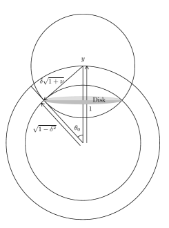
Figure 5: Illustration of the geometry for calculating $p_{0}$

Denote by $V_{t}$ and $A_{t}$ the volume and the surface area of a $t$-dimensional unit sphere, respectively. We have

$$V_{t}=\int_{0}^{1}A_{t}r^{t-1}dr=\frac{1}{t}A_{t}.$$

From the geometry of the situation as illustrated in Figure 5, $p_{0}$ is equal to the ratio of two areas $S_{1}$ and $S_{2}$. The first area $S_{1}$ is the portion of the surface area of the sphere of radius $\sqrt{1-\delta^{2}}$ and center $O$ contained within the sphere of radius $\delta\sqrt{1+\zeta}$ and center $y$. It is the surface area of a $(t-1)$-dimensional polar cap of radius $\sqrt{1-\delta^{2}}$ and polar angle $\theta_{0}$, and can be lower bounded by the area of a $(t-1)$-dimensional disk of radius $\sqrt{1-\delta^{2}}\sin\theta_{0}$, that is,

$$S_{1}\geq V_{t-1}\left(\sqrt{1-\delta^{2}}\sin\theta_{0}\right)^{t-1}=\frac{1}{t-1}A_{t-1}\left(\sqrt{1-\delta^{2}}\sin\theta_{0}\right)^{t-1}$$

The second area $S_{2}$ is simply the surface area of a $(t-1)$-dimensional sphere of radius $\sqrt{1-\delta^{2}}$

$$S_{2}=A_{t}\left(\sqrt{1-\delta^{2}}\right)^{t-1}.$$

Therefore, we obtain

$$p_{0} =\frac{S_{1}}{S_{2}}\geq\frac{\frac{1}{t-1}A_{t-1}\left(\sqrt{1-\delta^{2}}\sin\theta_{0}\right)^{t-1}}{A_{t}\left(\sqrt{1-\delta^{2}}\right)^{t-1}}=\frac{A_{t-1}}{(t-1)A_{t}}\left(\sin\theta_{0}\right)^{t-1}=\frac{\Gamma\left(\frac{t+1}{2}+\frac{1}{2}\right)}{\sqrt{\pi}t\Gamma\left(\frac{t+1}{2}\right)}\left(\sin\theta_{0}\right)^{t-1},$$

where we have used the well-known relationship between $A_{t-1}$ and $A_{t}$

$$\frac{A_{t-1}}{A_{t}}=\frac{1}{\sqrt{\pi}}\frac{(t-1)\Gamma\left(\frac{t}{2}+1\right)}{t\Gamma\left(\frac{t-1}{2}+1\right)}.$$

Now we need to calculate $\sin\theta_{0}$. By the law of cosines, we have

$$\cos\theta_{0}=\frac{1+1-\delta^{2}-\delta^{2}(1+\zeta)}{2\sqrt{1-\delta^{2}}}=\frac{1-\delta^{2}(1+\zeta/2)}{\sqrt{1-\delta}^{2}}$$

and it follows that

$$\sin^{2}\theta_{0}=1-\cos^{2}\theta_{0}=1-\frac{1+\delta^{4}(1+\zeta/2)^{2}-2\delta^{2}(1+\zeta/2)}{1-\delta^{2}}=\delta^{2}(1+\zeta)-\frac{\delta^{4}\zeta^{2}}{4(1-\delta^{2})}.$$

Now since $\zeta\leq 2(1-\delta^{2})$, we get

$$\sin\theta_{0}\geq\delta\sqrt{1+\zeta/2},$$

which completes the proof. ∎

Proof of Lemma A.6.

We first claim that

$$\mathbb{E}\left(\frac{S^{2}-n\sigma^{2}}{S}-\frac{\langle\theta,X\rangle}{\|X\|}\right)^{2}\leq\mathbb{E}\left(\frac{\|X\|^{2}-n\sigma^{2}}{\|X\|}-\frac{\langle\theta,X\rangle}{\|X\|}\right)^{2}.$$

In fact, writing $\mathbb{E}_{r}(\cdot)$ for the conditional expectation $\mathbb{E}(\cdot\,|\,\|X\|=r)$, it suffices to show that for $r<\sqrt{n\sigma^{2}}$ and $r>\sqrt{n\sigma^{2}}+c$

$$\mathbb{E}_{r}\left(\frac{S^{2}-n\sigma^{2}}{S}-\frac{\langle\theta,X\rangle}{\|X\|}\right)^{2}\leq\mathbb{E}_{r}\left(\frac{\|X\|^{2}-n\sigma^{2}}{\|X\|}-\frac{\langle\theta,X\rangle}{\|X\|}\right)^{2}.$$

When $r<\sqrt{n\sigma^{2}}$, it is equivalent to

$$\mathbb{E}_{r}\left(\frac{\langle\theta,X\rangle}{\|X\|}\right)^{2}\leq\mathbb{E}_{r}\left(\frac{\langle\theta,X\rangle}{\|X\|}-\frac{\|X\|^{2}-n\sigma^{2}}{\|X\|}\right)^{2}$$

It is then sufficient to show that $\mathbb{E}_{r}\langle\theta,X\rangle\geq 0$. This can be obtained by following a similar argument as in Lemma A.6 in [22]. When $r>\sqrt{n\sigma^{2}}+c$, we need to show that

$$\mathbb{E}_{r}\left(\frac{(\sqrt{n\sigma^{2}}+c)^{2}-n\sigma^{2}}{\sqrt{n\sigma^{2}}+c}-\frac{\langle\theta,X\rangle}{\|X\|}\right)^{2}\leq\mathbb{E}_{r}\left(\frac{\|X\|^{2}-n\sigma^{2}}{\|X\|}-\frac{\langle\theta,X\rangle}{\|X\|}\right)^{2},$$

which, after some algebra, boils down to

$$\frac{(\sqrt{n\sigma^{2}}+c)^{2}-n\sigma^{2}}{\sqrt{n\sigma^{2}}+c}+\frac{r^{2}-n\sigma^{2}}{r}\geq\frac{2}{r}\mathbb{E}_{r}\langle\theta,X\rangle.$$

This holds because

$$r\left(\frac{(\sqrt{n\sigma^{2}}+c)^{2}-n\sigma^{2}}{\sqrt{n\sigma^{2}}+c}+\frac{r^{2}-n\sigma^{2}}{r}-\frac{2}{r}\mathbb{E}_{r}\langle\theta,X\rangle\right)$$

$$\geq\|\theta\|^{2}+r^{2}-n\sigma^{2}-2\mathbb{E}_{r}\langle\theta,X\rangle$$

$$\geq\mathbb{E}_{r}\|X-\theta\|^{2}-n\sigma^{2}$$

$$\geq 0$$

where we have used the assumption that $r>\sqrt{n\sigma^{2}}+c$, $\|\theta\|\leq c$ and that

$$\mathbb{E}_{r}\|X-\theta\|\geq\mathbb{E}_{r}\|X\|-\|\theta\|\geq\sqrt{n\sigma^{2}}.$$

Now that we have shown (A.3) and noting that

$$\mathbb{E}\left(\frac{\|X\|^{2}-n\sigma^{2}}{\|X\|}-\frac{\langle\theta,X\rangle}{\|X\|}\right)^{2}=\sigma^{2}\mathbb{E}\left(\frac{\|X/\sigma\|^{2}-n}{\|X/\sigma\|}-\frac{\langle\theta/\sigma,X/\sigma\rangle}{\|X/\sigma\|}\right)^{2},$$

we can assume that $X\sim N(\theta,I_{n})$ and equivalently show that there exists a universal constant $C_{0}$ such that

$$\mathbb{E}\left(\frac{\|X\|^{2}-n}{\|X\|}-\frac{\langle\theta,X\rangle}{\|X\|}\right)^{2}\leq C_{0}$$

holds for any $n$ and $\theta$. Letting $Z=X-\theta$ and writing $\|\theta\|^{2}=\xi$, we have

$$\mathbb{E}\left(\frac{\|X\|^{2}-n}{\|X\|}-\frac{\langle\theta,X\rangle}{\|X\|}\right)^{2}$$

$$=\mathbb{E}\left(\frac{\|Z+\theta\|^{2}-n-\xi}{\|Z+\theta\|}-\frac{\langle\theta,Z\rangle}{\|Z+\theta\|}\right)^{2}$$

$$\leq 2\mathbb{E}\left(\frac{\|Z+\theta\|^{2}-n-\xi}{\|Z+\theta\|}\right)^{2}+2\mathbb{E}\left(\frac{\langle\theta,Z\rangle}{\|Z+\theta\|}\right)^{2}$$

$$\leq 2\mathbb{E}\|Z+\theta\|^{2}-4(n+\xi)+2\mathbb{E}\frac{(n+\xi)^{2}}{\|Z+\theta\|^{2}}+2\mathbb{E}\left(\frac{\langle\theta,Z\rangle}{\|Z+\theta\|}\right)^{2}$$

$$\leq 2(n+\xi)-4(n+\xi)+2\frac{(n+\xi)^{2}}{n+\xi-4}+2\mathbb{E}\left(\frac{\langle\theta,Z\rangle}{\|Z+\theta\|}\right)^{2}$$

$$=\frac{8(n+\xi)}{n+\xi-4}+2\mathbb{E}\left(\frac{\langle\theta,Z\rangle}{\|Z+\theta\|}\right)^{2}.$$

where the last inequality is due to Lemma A.11. To bound the last term, we apply the Cauchy-Schwarz inequality and get

$$\mathbb{E}\left(\frac{\langle\theta,Z\rangle}{\|Z+\theta\|}\right)^{2} \leq\sqrt{\mathbb{E}\frac{1}{\|Z+\theta\|^{4}}\mathbb{E}\langle\theta,Z\rangle^{4}}$$

$$\leq\sqrt{\frac{3(n-4)\xi^{2}}{(n-6)(n+\xi-4)(n+\xi-6)}}$$

where the last inequality is again due to Lemma A.11. Thus we just need to take $C_{0}$ to be

$$\sup_{n\geq 7,\xi\geq 0}\frac{8(n+\xi)}{n+\xi-4}+2\sqrt{\frac{3(n-4)\xi^{2}}{(n-6)(n+\xi-4)(n+\xi-6)}},$$

which is apparently a finite quantity. ∎

Proof of Lemma A.7.

Since the function $(x^{2}-n\sigma^{2})^{2}/x^{2}$ is decreasing on $(0,\sqrt{n\sigma^{2}})$ and increasing on $(\sqrt{n\sigma^{2}},\infty)$, we have

$$\frac{(S^{2}-n\sigma^{2})^{2}}{S^{2}}\leq\frac{(\|X\|^{2}-n\sigma^{2})^{2}}{\|X\|^{2}},$$

and it follows that if $n>4$

$$\mathbb{E}\frac{(S^{2}-n\sigma^{2})^{2}}{S^{2}} \leq\mathbb{E}\frac{(\|X\|^{2}-n\sigma^{2})^{2}}{\|X\|^{2}}$$ (A.18)

$$=\mathbb{E}\|X\|^{2}-2n\sigma^{2}+n^{2}\sigma^{4}\mathbb{E}\left(\frac{1}{\|X\|^{2}}\right)$$ (A.19)

$$\leq\|\theta\|^{2}-n\sigma^{2}+\frac{n^{2}\sigma^{4}}{\|\theta\|^{2}+n\sigma^{2}-4\sigma^{2}}$$ (A.20)

$$\leq\frac{\|\theta\|^{4}}{\|\theta\|^{2}+n\sigma^{2}}+\frac{4n}{n-4}\sigma^{2}$$ (A.21)

where (A.20) is due to Lemma A.11, and (A.21) is obtained by

$$\|\theta\|^{2}-n\sigma^{2}+\frac{n^{2}\sigma^{4}}{\|\theta\|^{2}+n\sigma^{2}-4\sigma^{2}}-\frac{\|\theta\|^{4}}{\|\theta\|^{2}+n\sigma^{2}}$$

$$=\frac{\|\theta\|^{4}+4\sigma^{2}(n\sigma^{2}-\|\theta\|^{2})}{\|\theta\|^{2}+n\sigma^{2}-4\sigma^{2}}-\frac{\|\theta\|^{4}}{\|\theta\|^{2}+n\sigma^{2}}$$

$$=\frac{4n^{2}\sigma^{6}}{(\|\theta\|^{2}+n\sigma^{2}-4\sigma^{2})(\|\theta\|^{2}+n\sigma^{2})}$$

$$\leq\frac{4n}{n-4}\sigma^{2}.$$

∎

Proof of Lemma A.8.

First, the second inequality

$$\mathbb{E}\|\widehat{\theta}_{+}-\theta\|^{2}\leq\frac{n\sigma^{2}\|\theta\|^{2}}{\|\theta\|^{2}+n\sigma^{2}}+4\sigma^{2}$$

is given by Lemma 3.10 from [22]. We thus focus on the first inequality. For convenience we write

$$g_{+}(x)=\left(\frac{\|x\|^{2}-n\sigma^{2}}{\|x\|^{2}}\right)_{+},\quad g_{\dagger}(x)=\frac{s(x)^{2}-n\sigma^{2}}{s(x)\|x\|}$$

with

$$s(x)=\begin{cases}\sqrt{n\sigma^{2}}&\text{if }\|x\|<\sqrt{n\sigma^{2}}\\ \sqrt{n\sigma^{2}}+c&\text{if }\|x\|>\sqrt{n\sigma^{2}}+c\\ \|x\|&\text{otherwise}\end{cases}.$$

Notice that $g_{+}(x)=g_{\dagger}(x)$ when $\|x\|\leq\sqrt{n\sigma^{2}}+c$ and $g_{+}(x)>g_{\dagger}(x)$ when $\|x\|>\sqrt{n\sigma^{2}}+c$. Since $g_{\dagger}$ and $g_{+}$ both only depend on $\|x\|$, we sometimes will also write $g_{\dagger}(\|x\|)$ for $g_{\dagger}(x)$ and $g_{+}(\|x\|)$ for $g_{+}(x)$. Setting $\mathbb{E}_{r}(\cdot)$ to denote the conditional expectation $\mathbb{E}(\cdot\,|\,\|X\|=r)$ for brevity, it suffices to show that for $r\geq\sqrt{n\sigma^{2}}+c$

$$\mathbb{E}_{r}\left(\|g_{\dagger}(X)X-\theta\|^{2}\right) \leq\mathbb{E}_{r}\left(\|g_{+}(X)X-\theta\|^{2}\right)$$

$$\Longleftrightarrow g_{\dagger}(r)^{2}r^{2}-2g_{\dagger}(r)\mathbb{E}_{r}\langle X,\theta\rangle \leq g_{+}(r)^{2}r^{2}-2g_{+}(r)\mathbb{E}_{r}\langle X,\theta\rangle$$

$$\Longleftrightarrow (g_{\dagger}(r)^{2}-g_{+}(r)^{2})r^{2} \geq 2(g_{\dagger}(r)-g_{+}(r))\mathbb{E}_{r}\langle X,\theta\rangle$$

$$\Longleftrightarrow (g_{\dagger}(r)+g_{+}(r))r^{2} \geq 2\mathbb{E}_{r}\langle X,\theta\rangle.$$ (A.22)

On the other hand, we have

$$(g_{\dagger}(r)+g_{+}(r))r^{2} \geq\left(\frac{\|\theta\|^{2}}{r^{2}}+\frac{r^{2}-n\sigma^{2}}{r^{2}}\right)r^{2}$$

$$=\|\theta\|^{2}+r^{2}-n\sigma^{2}$$

$$=\|\theta\|^{2}+r^{2}-2\mathbb{E}_{r}\langle X,\theta\rangle-n\sigma^{2}+2\mathbb{E}_{r}\langle X,\theta\rangle$$

$$=\mathbb{E}_{r}\|X-\theta\|^{2}-n\sigma^{2}+2\mathbb{E}_{r}\langle X,\theta\rangle$$

$$\geq 2\mathbb{E}_{r}\langle X,\theta\rangle$$

where the last inequality is because

$$\|X-\theta\|^{2}\geq(\|X\|-\|\theta\|)^{2}\geq n\sigma^{2}.$$

Thus, (A.22) holds and hence $\mathbb{E}\|\widehat{\theta}_{\dagger}-\theta\|^{2}\leq\mathbb{E}\|\widehat{\theta}_{+}-\theta\|^{2}$. ∎

Proof of Lemma A.9.

It is easy to see that $V_{1}\leq V_{2}$, because for any $\theta$ the inside minimum is smaller for ($A_{1}$) than for ($A_{2}$). Next, we will show $V_{1}\geq V_{2}$.

Suppose that $\theta^{*}$ achieves the value $V_{2}$, with corresponding $b^{*}$ and $\omega^{*}$. We claim that $\theta^{*}$ is non-increasing. In fact, if $\theta^{*}$ is not non-increasing, then there must exist an index $j$ such that $\theta_{j}^{*}<\theta_{j+1}^{*}$ and for simplicity let’s assume that $\theta^{*}_{1}<\theta^{*}_{2}$. We are going to show that this leads to $b^{*}_{1}=b^{*}_{2}$ and $\omega^{*}_{1}=\omega_{2}^{*}$. Write

$$s_{1}=\frac{\theta_{1}^{*4}}{\theta_{1}^{*2}+\varepsilon^{2}},\quad s_{2}=\frac{\theta_{2}^{*4}}{\theta_{2}^{*2}+\varepsilon^{2}}.$$

We have $s_{1}<s_{2}$. Let $\bar{b}^{*}=\frac{b_{1}^{*}+b_{2}^{*}}{2}$ and observe that $b_{1}^{*}\geq\bar{b}^{*}\geq b_{2}^{*}$. Notice that

$$\left(s_{1}2^{-2b_{1}^{*}}+s_{2}2^{-2b_{2}^{*}}\right)-\left(s_{1}2^{-2\bar{b}^{*}}+s_{2}2^{-2\bar{b}^{*}}\right)$$

$$=s_{1}\left(2^{-2b_{1}^{*}}-2^{-2\bar{b}^{*}}\right)+s_{2}\left(2^{-2b_{2}^{*}}-2^{-2\bar{b}^{*}}\right)$$

$$\geq s_{2}\left(2^{-2b_{1}^{*}}-2^{-2\bar{b}^{*}}\right)+s_{2}\left(2^{-2b_{2}^{*}}-2^{-2\bar{b}^{*}}\right)$$

$$\geq s_{2}\left(2^{-2b_{1}^{*}}+2^{-2b_{2}^{*}}-2\cdot 2^{-2\bar{b}^{*}}\right)$$

$$\geq 0,$$

where equality holds if and only if $b^{*}_{1}=b_{2}^{*}$, since $s_{2}>s_{1}\geq 0$. Hence, $b^{*}_{1}$ and $b_{2}^{*}$ have to be equal, or otherwise it would contradict with the assumption that $b^{*}$ achieves the inside minimum of ($A_{2}$). Now turn to $\omega^{*}$. Write $\bar{\omega}^{*}=\frac{\omega^{*}_{1}+\omega^{*}_{2}}{2}$ and note that $\omega_{1}^{*}\geq\bar{\omega}^{*}\geq\omega_{2}^{*}$. Consider

$$\left((1-\omega^{*}_{1})^{2}\theta_{1}^{*2}+\omega_{1}^{*2}\varepsilon^{2}\right)+\left((1-\omega^{*}_{2})^{2}\theta_{2}^{*2}+\omega_{2}^{*2}\varepsilon^{2}\right)-\left((1-\bar{\omega}^{*})^{2}(\theta_{1}^{*2}+\theta_{2}^{*2})+2\bar{\omega}^{*2}\varepsilon^{2}\right)$$

$$=\left((1-\omega_{1}^{*})^{2}-(1-\bar{\omega}^{*})^{2}\right)\theta_{1}^{*2}+\left((1-\omega_{2}^{*})^{2}-(1-\bar{\omega}^{*})^{2}\right)\theta_{2}^{*2}+\left(\omega_{1}^{*2}+\omega_{2}^{*2}-2\bar{\omega}^{*2}\right)\varepsilon^{2}$$

$$\geq\left((1-\omega_{1}^{*})^{2}-(1-\bar{\omega}^{*})^{2}\right)\theta_{2}^{*2}+\left((1-\omega_{2}^{*})^{2}-(1-\bar{\omega}^{*})^{2}\right)\theta_{2}^{*2}+\left(\omega_{1}^{*2}+\omega_{2}^{*2}-2\bar{\omega}^{*2}\right)\varepsilon^{2}$$

$$=\left((1-\omega_{1}^{*})^{2}+(1-\omega_{2}^{*})^{2}-2(1-\bar{\omega}^{*})^{2}\right)\theta_{2}^{*2}+\left(\omega_{1}^{*2}+\omega_{2}^{*2}-2\bar{\omega}^{*2}\right)\varepsilon^{2}$$

$$\geq 0,$$

where the equality holds if and only if $\omega_{1}^{*}=\omega_{2}^{*}$. Therefore, $\omega_{1}^{*}$ and $\omega_{2}^{*}$ must be equal. Now, with $b_{1}^{*}=b_{2}^{*}$ and $\omega_{1}^{*}=\omega_{2}^{*}$, we can switch $\theta_{1}^{*}$ and $\theta_{2}^{*}$ without increasing the objective function and violating the constraints. Thus, our claim that $\theta^{*}$ is non-increasing is justified.

Now that we have shown that the solution triplet $(\theta^{*},b^{*},\omega^{*})$ to ($A_{2}$) satisfy that $\theta^{*}$ is non-increasing, in order to prove $V_{1}\geq V_{2}$, it suffices to show that if we take $\theta=\theta^{*}$ in ($A_{1}$), the minimizer $b^{\star}$ is non-increasing and $b^{\star}_{1}\leq b_{\max}$. In fact, if so, we will have $b^{\star}=b^{*}$ as well as $\omega^{*}=\frac{\theta^{*2}_{j}}{\theta_{j}^{*2}+\varepsilon^{2}}$ and then

$$V_{1}\geq\min_{b:\sum_{j=1}^{N}b_{j}\leq B}\sum_{j=1}^{N}\left(\frac{\theta_{j}^{*4}}{\theta_{j}^{*2}+\varepsilon^{2}}2^{-2b_{j}}+\frac{\theta_{j}^{*2}\varepsilon^{2}}{\theta_{j}^{*2}+\varepsilon^{2}}\right)\geq V_{2}.$$

Let’s take $\theta=\theta^{*}$ in ($A_{1}$). The optimal $b^{\star}$ is non-increasing because the solution is given by the “reverse water-filling” scheme and $\theta^{*}$ is non-increasing. Next, we will show that $b^{\star}_{1}\leq b_{\max}$. If $b_{1}^{\star}>b_{\max}$, then we would have for $j=1,\dots,N$

$$\frac{\theta_{j}^{*4}}{\theta_{j}^{*2}+\varepsilon^{2}}2^{-2b^{\star}_{j}}\leq\frac{\theta_{1}^{*4}}{\theta_{1}^{*2}+\varepsilon^{2}}2^{-2b^{\star}_{1}}\leq\theta_{1}^{*2}2^{-2b_{\max}}\leq c^{2}2^{-4\log(1/\varepsilon)}=c^{2}\varepsilon^{4},$$

where the first inequality follows from the “reverse water-filling” solution, and therefore

$$\sum_{j=1}^{N}\frac{\theta_{j}^{*4}}{\theta_{j}^{*2}+\varepsilon^{2}}2^{-2b^{\star}_{j}}\leq Nc^{2}\varepsilon^{4}=o(\varepsilon^{\frac{4m}{2m+1}}),$$

which would not give the optimal solution. Hence, $b_{1}^{\star}\leq b_{\max}$, and this completes the proof. ∎

Lemma A.11.

Suppose that $W_{n,\xi}$ follows a non-central chi-square distribution with $n$ degrees of freedom and non-centrality parameter $\xi$. We have for $n\geq 5$

$$\mathbb{E}\left(W_{n,\xi}^{-1}\right)\leq\frac{1}{n+\xi-4},$$

and for $n\geq 7$

$$\mathbb{E}\left(W_{n,\xi}^{-2}\right)\leq\frac{n-4}{(n-6)(n+\xi-4)(n+\xi-6)}.$$

Proof.

It is well known that the non-central chi-square random variable $W_{n,\xi}$ can be written as a Poisson-weighted mixture of central chi-square distributions, i.e., $W_{n,\xi}\sim\chi^{2}_{n+2K}$ with $K\sim\text{Poisson}(\xi/2)$. Then

$$\mathbb{E}\left(W_{n,\xi}^{-1}\right) =\mathbb{E}\left(\mathbb{E}(W_{n,\xi}^{-1}\,|\,K)\right)=\mathbb{E}\left(\frac{1}{n+2K-2}\right)$$

$$\geq\frac{1}{n+2\mathbb{E}K-2}=\frac{1}{n+\xi-2}$$

where we have used the fact that $\mathbb{E}(1/\chi^{2}_{n})=n-2$ and Jensen’s inequality. Similarly, we have

$$\mathbb{E}\left(W_{n,\xi}^{-2}\right) =\mathbb{E}\left(\mathbb{E}(W_{n,\xi}^{-2}\,|\,K)\right)=\mathbb{E}\left(\frac{1}{(n+2K-2)(n+2K-4)}\right)$$

$$\geq\frac{1}{(n+2\mathbb{E}K-2)(n+2\mathbb{E}K-4)}$$

$$=\frac{1}{(n+\xi-2)(n+\xi-4)}$$

Using the Poisson-weighted mixture representation, the following recurrence relation can be derived [7]

$$1 =\xi\mathbb{E}\left(W_{n+4,\xi}^{-1}\right)+n\mathbb{E}\left(W^{-1}_{n+2,\xi}\right),$$ (A.23)

$$\mathbb{E}\left(W^{-1}_{n,\xi}\right) =\xi\mathbb{E}\left(W_{n+4,\xi}^{-2}\right)+n\mathbb{E}\left(W^{-2}_{n+2,\xi}\right),$$ (A.24)

for $n\geq 3$. Thus,

$$\mathbb{E}\left(W_{n+4,\xi}^{-1}\right) =\frac{1}{\xi}-\frac{n}{\xi}\mathbb{E}\left(W^{-1}_{n+2,\xi}\right)$$

$$\leq\frac{1}{\xi}-\frac{n}{\xi}\frac{1}{n+\xi}$$

$$=\frac{1}{n+\xi}.$$

Replacing $n$ by $n-4$ proves (A.11). On the other hand, rearranging (A.23), we get

$$\mathbb{E}\left(W^{-1}_{n+2,\xi}\right) =\frac{1}{n}-\frac{\xi}{n}\mathbb{E}\left(W^{-1}_{n+4,\xi}\right)$$

$$\leq\frac{1}{n}-\frac{\xi}{n}\frac{1}{n+\xi+2}$$

$$=\frac{n+2}{n(n+\xi+2)}.$$

Now using (A.24), we have

$$\mathbb{E}\left(W_{n+4,\xi}^{-2}\right) =\frac{1}{\xi}\mathbb{E}\left(W^{-1}_{n,\xi}\right)-\frac{n}{\xi}\mathbb{E}\left(W^{-2}_{n+2,\xi}\right)$$

$$\leq\frac{n}{\xi(n-2)(n+\xi)}-\frac{n}{\xi(n+\xi)(n+\xi-2)}$$

$$=\frac{n}{(n-2)(n+\xi)(n+\xi-2)}.$$

Replacing $n$ by $n-4$ proves (A.11). ∎

References

- [1] Rudolf Ahlswede and MV Burnashev. On minimax estimation in the presence of side information about remote data. Ann. Statist., pages 141–171, 1990.
- [2] Rudolf Ahlswede and Imre Csiszár. Hypothesis testing with communication constraints. IEEE Trans. Inform. Theory, 32(4):533–542, 1986.
- [3] Toby Berger, Zhen Zhang, and Harish Viswanathan. The CEO problem. IEEE Trans. Inform. Theory, 42(3):887–902, 1996.
- [4] Lawrence D Brown, Mark G Low, et al. Asymptotic equivalence of nonparametric regression and white noise. Ann. Statist., 24(6):2384–2398, 1996.
- [5] John J Bruer, Joel A Tropp, Volkan Cevher, and Stephen Becker. Time–data tradeoffs by aggressive smoothing. In Advances in Neural Information Processing Systems, pages 1664–1672, 2014.
- [6] Venkat Chandrasekaran and Michael I Jordan. Computational and statistical tradeoffs via convex relaxation. Proc. Natl. Acad. Sci. USA, 110(13):E1181–E1190, 2013.
- [7] R Chattamvelli and MC Jones. Recurrence relations for noncentral density, distribution functions and inverse moments. J. Stat. Comput. Simul., 52(3):289–299, 1995.
- [8] Thomas M Cover and Joy A Thomas. Elements of Information Theory. Wiley-Interscience, 2006.
- [9] David L Donoho. Wald lecture I: Counting bits with Kolmogorov and Shannon. Note for the Wald Lectures, 1997.
- [10] Stark C Draper and Gregory W Wornell. Side information aware coding strategies for sensor networks. IEEE Journal on Selected Areas in Communications, 22(6):966–976, 2004.
- [11] Sameh Galal and Mark Horowitz. Energy-efficient floating-point unit design. IEEE Trans. Comput., 60(7):913–922, 2011.
- [12] Robert G Gallager. Information Theory and Reliable Communication. John Wiley & Sons, 1968.
- [13] Ankit Garg, Tengyu Ma, and Huy Nguyen. On communication cost of distributed statistical estimation and dimensionality. In Advances in Neural Information Processing Systems, pages 2726–2734, 2014.
- [14] Te Sun Han and Shun-ichi Amari. Statistical inference under multiterminal data compression. IEEE Trans. Inform. Theory, 44(6):2300–2324, 1998.
- [15] Iain M Johnstone. Gaussian estimation: Sequence and wavelet models. Unpublished manuscript, 2015.
- [16] Mario Lucic, Mesrob I Ohannessian, Amin Karbasi, and Andreas Krause. Tradeoffs for space, time, data and risk in unsupervised learning. In International Conference on Artificial Intelligence and Statistics, 2015.
- [17] Michael Nussbaum. Spline smoothing in regression models and asymptotic efficiency in . Ann. Statist., 13(3):984–997, 1985.
- [18] Michael Nussbaum. Asymptotic equivalence of density estimation and gaussian white noise. Ann. of Statist., pages 2399–2430, 1996.
- [19] Michael Nussbaum. Minimax risk: Pinsker bound. Encyclopedia of Statistical Sciences, 3:451–460, 1999.
- [20] Maxim Raginsky. Learning from compressed observations. In IEEE Information Theory Workshop, pages 420–425, 2007.
- [21] D Sakrison. A geometric treatment of the source encoding of a Gaussian random variable. IEEE Trans. Inform. Theory, 14(3):481–486, 1968.
- [22] Alexandre B Tsybakov. Introduction to Nonparametric Estimation. Springer Series in Statistics, 1st edition, 2008.
- [23] Ramji Venkataramanan, Tuhin Sarkar, and Sekhar Tatikonda. Lossy compression via sparse linear regression: Computationally efficient encoding and decoding. In IEEE International Symposium on Information Theory (ISIT), pages 1182–1186. IEEE, 2013.
- [24] Yuchen Zhang, John Duchi, Michael I Jordan, and Martin J Wainwright. Information-theoretic lower bounds for distributed statistical estimation with communication constraints. In Advances in Neural Information Processing Systems, pages 2328–2336, 2013.
- [25] Zhen Zhang and Toby Berger. Estimation via compressed information. IEEE Trans. Inform. Theory, 34(2):198–211, 1988.
- [26] Shuheng Zhou, John Lafferty, and Larry Wasserman. Compressed and privacy-sensitive sparse regression. IEEE Trans. Inform. Theory, 55(2):846–866, 2009.
- [27] Yuancheng Zhu and John Lafferty. Quantized estimation of Gaussian sequence models in euclidean balls. In Advances in Neural Information Processing Systems, pages 3662–3670, 2014.