Mathematical Modelling, Simulation, and Optimal Control of the 2014 Ebola Outbreak in West Africa

Abstract

The Ebola virus is currently one of the most virulent pathogens for humans. The latest major outbreak occurred in Guinea, Sierra Leone and Liberia in 2014. With the aim of understanding the spread of infection in the affected countries, it is crucial to modelize the virus and simulate it. In this paper, we begin by studying a simple mathematical model that describes the 2014 Ebola outbreak in Liberia. Then, we use numerical simulations and available data provided by the World Health Organization to validate the obtained mathematical model. Moreover, we develop a new mathematical model including vaccination of individuals. We discuss different cases of vaccination in order to predict the effect of vaccination on the infected individuals over time. Finally, we apply optimal control to study the impact of vaccination on the spread of the Ebola virus. The optimal control problem is solved numerically by using a direct multiple shooting method.

1 Introduction

Ebola is a lethal virus for humans. It was previously confined to Central Africa but recently was also identified in West Africa [1]. As of October 8, 2014, the World Health Organization (WHO) reported 4656 cases of Ebola virus deaths, with most cases occurring in Liberia [2]. The extremely rapid increase of the disease and the high mortality rate make this virus a major problem for public health. Typically, patients present fever, malaise, abdominal, headache, and asthenia. One week after the onset of symptoms, a rash often appears followed by haemorrhagic complications, leading to death after an average of 10 days in 50%–90% of infections [3, 4, 5, 6]. Ebola is transmitted through direct contact with blood, bodily secretions and tissues of infected ill or dead humans and non-human primates [7, 8, 9].

The main aim of this work is to understand the dynamics of the Liberian population infected by Ebola virus in 2014, by using an appropriate mathematical model. More precisely, we begin by considering a system of ordinary differential equations to describe the 2014 Ebola outbreak, which is nothing else than an epidemic SIR model, that is, a model based on the division of the population into three groups: the Susceptible, the Infected, and the Recovered [10, 11, 12]. We simulate the model obtained by parameters estimated on November 4, 2014, by Kaurov [13]. Our objectives are to better understand the outbreak and to predict the effect of vaccination on the infected individuals over time.

In order to deal with the epidemic of Ebola, governments have decided to implement tough measures. For example, some have applied quarantine procedures while others have opted for mass vaccination plans as a precaution to the epidemic [14, 15, 16, 17]. In this context, we consider an optimal control problem to study the effect of vaccination on the spread of virus.

The text is organized as follows. In Section 2 we introduce a basic mathematical model to describe the dynamics of the Ebola virus during the 2014 outbreak in Liberia. After the mathematical modelling, we use the obtained model to simulate it in Section 3 with the parameters estimated from recent statistical data based on the WHO report of the 2014 Ebola outbreak [18]. Following [13], in Section 4 we study different cases of vaccination of individuals by adding a vaccination term to the model. Section 5 presents an optimal control problem, which we use to study the impact of a vaccination campaign on the spread of the virus. We end with Section 6 of conclusions and future work, where the results are summarized and some research perspectives presented.

2 The Basic Mathematical Model

The objective of this section is to describe mathematically the dynamics of the population infected by the Ebola virus. The dynamics is described by a system of differential equations. This system is based on the common SIR (Susceptible-Infectious-Recovery) epidemic model, where the population is divided into three groups: the susceptible group, denoted by $S(t)$, the infected group, denoted by $I(t)$, and the recovered group, denoted by $R(t)$. The total population, assumed constant during the short period of time under study, is given by $N=S(t)+I(t)+R(t)$.

To create the equations that describe the population of each group along time, let us start with the fact that the population of the susceptible group will be reduced as the infected come into contact with them with a rate of infection $\beta$. This means that the change in the population of susceptible is equal to the negative product of $\beta$ with $S(t)$ and $I(t)$:

$$\dfrac{dS(t)}{dt}=-\beta\dfrac{S(t)I(t)}{N}.$$ (1)

Now, let us create the equation that describes the infected group over time, knowing that the population of this group changes in two ways:

(i)

people leave the susceptible group and join the infected group, thus adding to the total population of infected a term $\beta S(t)I(t)$;

(ii)

people leave the infected group and join the recovered group, reducing the infected population by $-\mu I(t)$.

This is written as

$$\dfrac{dI(t)}{dt}=\beta\dfrac{S(t)I(t)}{N}-\mu I(t).$$ (2)

Finally, the equation that describes the recovery population is based on the individuals recovered from the virus at rate $\mu$. This means that the recovery group is increased by $\mu$ multiplied by $I(t)$:

$$\dfrac{dR(t)}{dt}=\mu I(t).$$ (3)

Figure 1 shows the relationship between the three variables of our SIR model.

Figure 1: The scheme of the Susceptible-Infected-Recovered model (1)–(3).

As shown in the next section, this simple model describes well the 2014 Ebola outbreak in Liberia for suitable chosen parameters $\beta$ and $\mu$ and appropriate initial conditions $S(0)$, $I(0)$ and $R(0)$.

3 Numerical Simulations of the Basic Model and Discussion

With the aim to approximate the 2014 Ebola outbreak in Liberia, we now simulate the complete set of equations (1)–(3) that describe the SIR model:

$$\begin{cases}\dfrac{dS(t)}{dt}=-\beta\dfrac{S(t)I(t)}{N},\\[8.5359pt] \dfrac{dI(t)}{dt}=\beta\dfrac{S(t)I(t)}{N}-\mu I(t),\\[8.5359pt] \dfrac{dR(t)}{dt}=\mu I(t),\end{cases}$$ (4)

where $\beta$ is the rate of infection and $\mu$ the rate of recovery. The data for the outbreak in Liberia is based on the cumulative numbers of total reported cases (confirmed and probable) taken from the official data reported by the Ministry of Health of Liberia up to October 26, 2014, as provided by the World Health Organisation (WHO) [18] (in particular, the Ebola virus disease cases reported each week from Liberia are given in Figure 2 of [19]). The model fits well the reported data of confirmed (means infected) cases in Liberia. Note that the exact population size $N$ does not need to be known to estimate the model parameters as long as the number of cases is small compared to the total population size [20]. To estimate the parameters of the model, we adapted the initialisation of $S$ and $I$ with the reported data of [19] by fitting the actual data of confirmed cases in Liberia. The data that we are studying is the number of individuals with confirmed infection between July 14 and October 12, 2014. The result of fitting is shown in Figure 2.

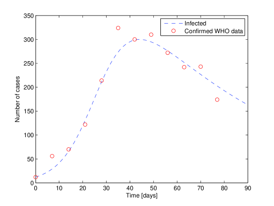
Figure 2: Graph of Infected $I(t)$ obtained from (4) with $\beta=0.000318$, $\mu=0.0175$, $S(0)=460$, $I(0)=12$, and $R(0)=0$ versus the real data of confirmed cases for the 2014 Ebola outbreak occurred in Liberia from July 14 (day $t=0$) and October 12, 2014 (day $t=90$).

The comparison between the curve of infected obtained by our simulation and the reported data of confirmed cases by WHO shows that the mathematical model (4) fits well the real data by using $\beta=0.000318$ as the rate of infection and $\mu=0.0175$ as the rate of recovery. The initial numbers of susceptible, infected, and recovered groups, are given by $S(0)=460$, $I(0)=12$, and $R(0)=0$, respectively. The choice of $S(0)$ is in agreement with the data shown in Figure 2 of [19], as the biggest value in the histogram is 460. To interpret the simulation results, we describe the evolution of each group of individuals over time and the link between them. Figure 3 shows that the susceptible group begins to plummet and, simultaneously, the number of infected begins to rise. This is due to how infectious the Ebola virus is.

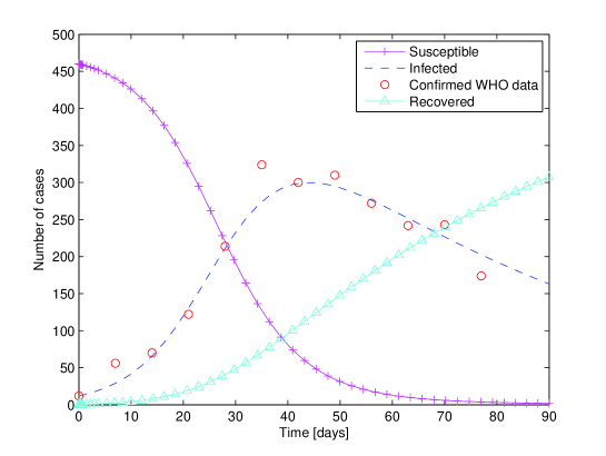
Figure 3: The evolution of susceptible ($S(t)$), infected ($I(t)$), and recovered ($R(t)$) for the period July 14 ($t=0$) and October 12, 2014 ($t=90$), given by the Ebola Liberia model (4) with $\beta=0.000318$, $\mu=0.0175$, $S(0)=460$, $I(0)=12$, and $R(0)=0$. The real data of confirmed cases for the 2014 Ebola outbreak occurred in Liberia, taken from [18], is shown with circles.

When we compare our results with those of Astacio et al. [21], when they modeled the 1976 outbreak of Ebola in Yambuku, a small village in Mongala District in northern Democratic Republic of Congo (previously Zaire), and the 1995 outbreak of Ebola in Kikwit, in the southwestern part of the Democratic Republic of Congo, we note that the evolution of each group obtained in our simulations is reasonable. The main difference between the 2014 outbreak of Ebola in Liberia and the previous outbreaks of Ebola in Yambuku and Kikwit studied in [21] is at the end of the evolution of infected: while in the previous 1976 and 1995 outbreaks of Ebola in Yambuku and Kikwit the infected group goes to zero, now in the 2014 outbreak of Ebola in Liberia the infected group remains important with a high number of infected individuals by the virus, which describes the reality of what is currently happening in Liberia. One can conclude that the 2014 Ebola outbreak of Liberia is much more dangerous than the previous Ebola outbreaks.

4 Modelling and Simulation of Ebola Outbreak with Vaccination

In this section, we simulate the model by using parameters estimated on November 4, 2014, by Kaurov [13], who studied statistically the recent data of the World Health Organisation (WHO) [18]. In his statistical study, Kaurov studied the outbreak by modeling it with Wolfram’s Mathematica language. Here we use his SIR model for modelling and time-discrete equations for resolution of the set of equations through Matlab.

4.1 The Basic Model with Kaurov’s Estimation of Parameters

Let us recall the complete set of equations considered by [13]:

$$\begin{cases}\dfrac{dS(t)}{dt}=-\beta S(t)I(t),\\[8.5359pt] \dfrac{dI(t)}{dt}=\beta S(t)I(t)-\mu I(t),\\[8.5359pt] \dfrac{dR(t)}{dt}=\mu I(t),\end{cases}$$ (5)

where, as before, $\beta$ is the rate of infection and $\mu$ is the rate of recovery. The parameters obtained by Kaurov, knowing that 95% of population is susceptible and 5% of population is infected, are $\beta=0.2$ and $\mu=0.1$ [13]. In agreement, the initial susceptible, infected, and recovered populations are given, respectively, by $S(0)=0.95$, $I(0)=0.05$, and $R(0)=0$ (note that in contrast with Sections 2 and 3, the variables are now dimensionless).

Our numerical simulations were done with the ODE solver of Matlab. The results are shown in Figure 4. To interpret the results, we describe the evolution of each group over time and the links between them. Figure 4 shows that the susceptible group begins to plummet due to how infectious the virus is and, simultaneously, the infected group’s number begins to rise.

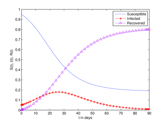
Figure 4: Solution to the 2014 outbreak Ebola model (5) with $\beta=0.2$, $\mu=0.1$, $S(0)=0.95$, $I(0)=0.05$, and $R(0)=0$.

An important dimensionless quantity that plays a key role in any SIR model is the well-known basic reproduction number $R_{0}$ [22]. This number tells us how fast the disease will spread at the epidemic. For model (5), the basic reproduction number is simply given by $\beta/\mu$. Let us now discuss the comparison between the different values of $R_{0}$ obtained recently. On September 2, 2014, Althaus studied the case of the 2014 Ebola outbreak occurred in Guinea, in Sierra Leone, and in Liberia [20]. In his study, Althaus used the WHO data occurred in the three countries. He found different values for the basic reproduction number, depending on the country: in Guinea $R_{0}=1.51$, in Sierra Leone the value of $R_{0}$ is given by $2.53$, while in Liberia $R_{0}$ is equal to $1.59$. Let us now compare between these values and the value for the basic reproduction number studied by Kaurov, knowing that his study, which was done on November 4, 2014, is more recent than the one of Althaus, done September 2, 2014. As the parameters estimated statistically by Kaurov are for the three countries, our comparison will be between $R_{0,A}$, the mean of the three basic reproduction numbers found by Althaus, and $R_{0,K}$, the number found more recently by Kaurov. The value of $R_{0,A}$ is given by $1.876$, where the more recent $R_{0,K}$ is given by $2$. We claim that the basic reproduction number increased between September and November 2014.

4.2 Dynamics in Case of Vaccination

Infectious diseases have tremendous influence on human life. In last decades, controlling infectious diseases has been an increasingly complex issue. A strategy to control infectious diseases is through vaccination. Now our idea is to study the effect of vaccination in practical Ebola situations. The case of the French nurse cured of Ebola with the help of an experimental vacine is a proof of the possibility of treatment by vaccinating infected individuals [23].

In this section, we improve the SIR model described in Section 4.1. The system of equations that describe the Susceptible-Infectious-Recovery (SIR) model with vaccination is:

$$\begin{cases}\dfrac{dS(t)}{dt}=-\beta S(t)I(t)-\upsilon S(t),\\[8.5359pt] \dfrac{dI(t)}{dt}=\beta S(t)I(t)-\mu I(t),\\[8.5359pt] \dfrac{dR(t)}{dt}=\mu I(t)+\upsilon S(t),\end{cases}$$ (6)

where $\beta$ is the rate of infection, $\mu$ is the rate of recovery, and $\upsilon$ is the percentage of individuals vaccinated every day [24]. Figure 5 shows the relationship between the variables of the SIR model with vaccination (6).

Figure 5: The scheme of the Susceptible-Infected-Recovered model with vaccination (6).

4.3 Numerical Simulation in Case of Vaccination

We simulate the SIR model with vaccination (6) in order to predict the evolution of every group of individuals in case of vaccination. Our study is based in the test of different rates of vaccinations and their effect on the curve of every group.

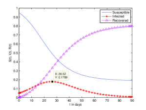
(a) $\upsilon=0$

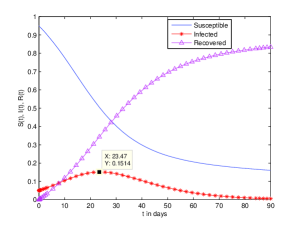
(b) $\upsilon=0.005$

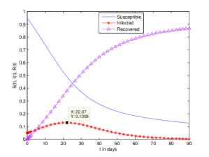
(c) $\upsilon=0.01$

Figure 6: A solution to the SIR model (6) with $\beta=0.2$, $\mu=0.1$, $S(0)=0.95$, $I(0)=0.05$, $R(0)=0$, and different rates of vaccination: $\upsilon=0$ (a), $\upsilon=0.005$ (b), and $\upsilon=0.01$ (c).

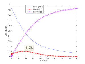
(a) $\upsilon=0.02$

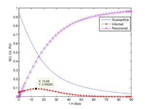
(b) $\upsilon=0.03$

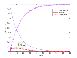
(c) $\upsilon=0.06$

Figure 7: A solution to the SIR model (6) with $\beta=0.2$, $\mu=0.1$, $S(0)=0.95$, $I(0)=0.05$, $R(0)=0$, and different rates of vaccination: $\upsilon=0.02$ (a), $\upsilon=0.03$ (b), and $\upsilon=0.06$ (c).

The results are shown in Figures 6 and 7. These figures present different rates of vaccination and their effect on the peak of the curve of infected individuals along time. The time-dependent curve of infected individuals shows that when the percentage of vaccinated individuals increases, the peak of the curve of infected individuals is less important and the period of infection (the corresponding number of days) is shorter while the number of recovered gets more important. In fact, in case of infection without vaccination, the curve of the infected group goes to zero in about 90 days (see Figure 6), where in the presence of vaccination the curve of the infected group goes to zero in about 45 days (see Figure 7). This shows the efficiency of using vaccination in controlling Ebola. Table 1 presents the maximum percentage of infected individuals, corresponding to different rates of vaccinations, and the respective number of days for the peak of infected.

Rate of vaccination	Maximum percentage	Days to the peak of
	of infected	$I(t)$
$0$	$17\%$	$26.52$
$0.005$	$15\%$	$23.47$
$0.01$	$13\%$	$22.07$
$0.02$	$10\%$	$17.09$
$0.03$	$9\%$	$13.68$
$0.06$	$7\%$	$9.28$

Table 1: Maximum percentage of infected individuals $I$ corresponding to different rates $\upsilon$ of vaccination and respective number of days for the peak of $I$.

5 The Optimal Control Problem

Optimal control has been recently used with success in a series of epidemiological problems: see [17, 25, 26, 27] and references therein. In this section, we present an optimal control problem by introducing into the model (5) a control $u(t)$ representing the vaccination rate at time $t$. The control $u(t)$ is the fraction of susceptible individuals being vaccinated per unit of time. We assume that all susceptible individuals that are vaccinated are transferred directly to the removed class. Then, the mathematical model with control is given by the following system of nonlinear differential equations:

$$\begin{cases}\dfrac{dS(t)}{dt}=-\beta S(t)I(t)-u(t)S(t),\\[8.5359pt] \dfrac{dI(t)}{dt}=\beta S(t)I(t)-\mu I(t),\\[8.5359pt] \dfrac{dR(t)}{dt}=\mu I(t)+u(t)S(t),\end{cases}$$ (7)

where $S(0)\geq 0$, $I(0)\geq 0$, and $R(0)\geq 0$ are given. Our goal is to reduce the infected individuals and the cost of vaccination. Precisely, our optimal control problem consists of minimizing the objective functional

$$J(u)=\int_{0}^{t_{f}}I(t)+\dfrac{A}{2}u^{2}(t)dt,$$ (8)

subject to $0\leq u(t)\leq 0.9$ for $t\in[0,t_{f}]$, where the parameters $A\geq 0$ and $t_{f}$ denote, respectively, the weight on cost and the duration of the vaccination program. We present the numerical solution to this optimal control problem, comparing the results with the numerical simulation results obtained in Section 4 via Matlab. As in Section 4, the rate of infection is given by $\beta=0.2$, the recovered rate is given by $\mu=0.1$, and we use $S(0)=0.95$, $I(0)=0.05$, and $R(0)=0$ for the initial number of susceptible, infected, and recovered populations, respectively (i.e., at the beginning 95% of population is susceptible and 5% is already infected with Ebola). Note that when $u(t)\equiv 0$ model (7) reduces to (5); and when $u(t)\equiv\upsilon$ model (7) reduces to (6).

The numerical simulation of the system without control ($u(t)\equiv 0$) was done with Matlab in Section 4.1. For our numerical solution of the optimal control problem, we have used the ACADO solver [28], which is based on a multiple shooting method, including automatic differentiation and based ultimately on the semidirect multiple shooting algorithm of Bock and Pitt [29]. ACADO is a self-contained public domain software environment written in C++ for automatic control and dynamic optimization.

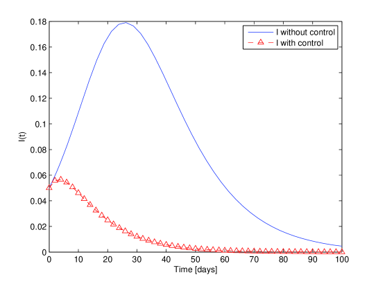
Figure 8: The function $I(t)$ of infected individuals with and without control.

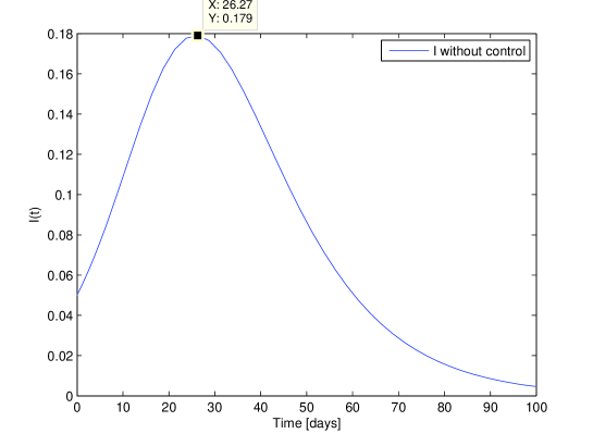
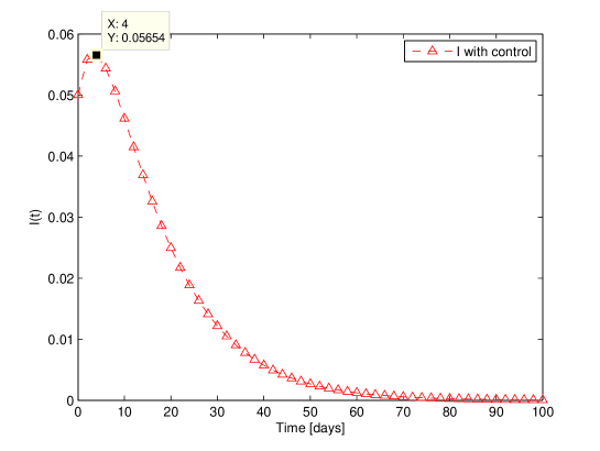
Figure 9: Comparison between the peaks of infected individuals $I(t)$ in case of optimal control versus without control.

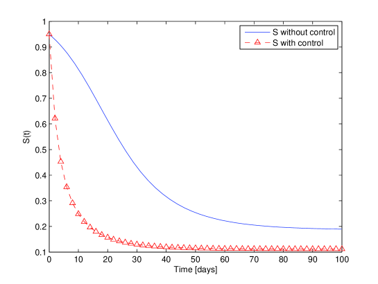
Figure 10: Susceptible individuals $S(t)$ in case of optimal control versus without control.

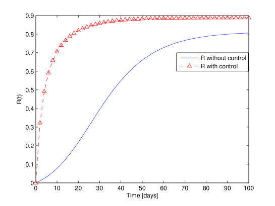
Figure 11: Recovered individuals $R(t)$ in case of optimal control versus without control.

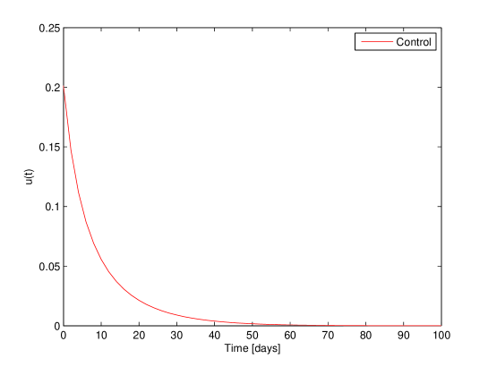
Figure 12: The optimal control $u$ for problem (7)–(8).

Figures 8 and 9 show the significant difference in the number of infected individuals with and without control. In fact, in case of optimal control, the function $I$ decreases greatly: the maximum value on the infected curve $I$ under optimal control is 5.6% against 17.9% without any control (see Figure 9).

In Figure 10, we see that the number of susceptible $S$ decreases more rapidly during the vaccination campaign. It reaches 11% at the end of the campaign against 19% in the absence of optimal control.

Figure 11 shows that the number of recovered individuals increases rapidly. The number $R(t_{f})$ at the end of the optimal control vaccination period is 88.7% instead of 80.5% without control. Figure 12 gives a representation of the optimal control $u(t)$.

6 Conclusion

We investigated a mathematical model that provides a good description of the 2014 Ebola outbreak in Liberia: the model fits well the data of confirmed cases in Liberia provided by the World Health Organization. The evolution of infected individuals shows that the infected population remains important, describing the actual evolution of the virus in Liberia. This evolution is different than Ebola’s outbreak in the last decades. Our study of the SIR model with vaccination shows that vaccination is a very efficient factor in reducing the number of infected individuals in a short period of time and increasing the number of recovered individuals. We also discussed an optimal control problem related to the impact of a vaccination strategy on the spread of the 2014 outbreak of Ebola in West Africa. The numerical simulation of both systems, with and without control, shows that an optimal control strategy greatly helps to reduce the number of infected and susceptible individuals and increases the number of recovered individuals.

As future work, we plan to include in our study other factors. In particular, we intend to include in the mathematical model the treatment of infected individuals with a quarantine procedure. Another interesting line of research is to investigate the effect of impulsive vaccination.

References

- [1] M. Barry, F. A. Traoré, F. B. Sako, D. O. Kpamy, E. I. Bah, M. Poncin, S. Keita, M. Cisse, A. Touré. Ebola outbreak in Conakry, Guinea: Epidemiological, clinical, and outcome features. Médecine et Maladies Infectieuses 44 (2014), no. 11–12, 491–494.
- [2] J. A. Lewnard, M. L. Ndeffo Mbah, J. A. Alfaro-Murillo, F. L. Altice, L. Bawo, T. G. Nyenswah, A. P. Galvani. Dynamics and control of Ebola virus transmission in Montserrado, Liberia: a mathematical modelling analysis. The Lancet Infectious Diseases 14 (2014), no. 12, 1189–1195.
- [3] WHO, Report of an International Study Team. Ebola haemorrhagic fever in Sudan 1976. Bull. World Health Organ. 56 (1978), no. 2, 247–270.
- [4] Report of an International Commission. Ebola haemorrhagic fever in Zaire, 1976. Bull. World Health Organ. 56 (1978), no. 2, 271–293.
- [5] Uganda Ministry of Health. An outbreak of Ebola in Uganda. Trop. Med. Int. Health. 7 (2002), no. 12, 1068–1075.
- [6] J. Legrand, R. F. Grais, P. Y. Boelle, A. J. Valleron, A. Flahault. Understanding the dynamics of Ebola epidemics. Epidemiol. Infect. 135 (2007), no. 4, 610–621.
- [7] S. F. Dowell, R. Mukunu, T. G. Ksiazek, A. S. Khan, P. E. Rollin, C. J. Peters. Transmission of Ebola hemorrhagic fever: a study of risk factors in family members, Kikwit, Democratic Republic of the Congo, 1995. Commission de Lutte contre les Epidémies à Kikwit. J. Infect. Dis. 179 (1999), Suppl. 1, S87–S91.
- [8] L. Borio et al. [Working Group on Civilian Biodefense; Corporate Author]. Hemorrhagic fever viruses as biological weapons: medical and public health management. Journal of the American Medical Association 287 (2002), no. 18, 2391–2405.
- [9] C. J. Peters, J. W. LeDuc. An introduction to Ebola: the virus and the disease. Journal of Infectious Diseases 179 (Suppl. 1), 1999.
- [10] G. Chowell, J. M. Hayman, L. M. A. Bettencourt, C. Castillo-Chavez. Mathematical and Statistical Estimation Approaches in Epidemiology, Springer, Dordrecht, 2009.
- [11] D. Zeng, H. Chen, C. Castillo-Chavez, W. B. Lober, M. Thurmond. Infectious Disease Informatics and Biosurveillance. Integrated Series in Information Systems, Vol. 27, Springer, New York, 2011.
- [12] G. Chowell, N. W. Hengartner, C. Castillo-Chavez, P. W. Fenimore, J. M. Hyman. The basic reproductive number of Ebola and the effects of public health measures: the cases of Congo and Uganda. Journal of Theoretical Biology 229 (2004), no. 1, 119–126.
- [13] V. Kaurov. Modeling a Pandemic like Ebola with the Wolfram Language. Technical Communication & Strategy, November 4, 2014. http://blog.wolfram.com/2014/11/04/modeling-a-pandemic-like-ebola-with-the-wolfram-language
- [14] C. P. Farrington, M. N. Kanaan. Branching process models for surveillance of infectious diseases controlled by mass vaccination. Biostatistics 4 (2003), no. 2, 279–295.
- [15] Forum on Medical and Public Health Preparedness for Catastrophic Events. The 2009 Influenza Vaccination Campaign, Summary of a Workshop Series, The National Academies Press, Washington, D.C., 2010.
- [16] W. Robert. Tindle Vaccines for Human Papillomavirus Infection and Disease Medical Intelligence Unit. Medical Intelligence Unit, R. G., Landes Company, Austin, Texas, 1999.
- [17] H. S. Rodrigues, M. T. T. Monteiro, D. F. M. Torres. Vaccination models and optimal control strategies to dengue. Math. Biosci. 247 (2014), 1–12. arXiv:1310.4387
- [18] WHO, World Health Organization. Ebola response roadmap – Situation report update. Last time accessed: October 2014. http://www.who.int/csr/disease/ebola/situation-reports/en
- [19] WHO, World Health Organisation, Ebola response roadmap situation report, 29 October 2014, http://apps.who.int/iris/bitstream/10665/137376/1/roadmapsitrep_29Oct2014_eng.pdf?ua=1
- [20] C. L. Althaus. Estimating the Reproduction Number of Ebola Virus (EBOV) During the 2014 Outbreak in West Africa. PLOS Currents Outbreaks, September 2, 2014. http://dx.doi.org/10.1371/currents.outbreaks.91afb5e0f279e7f29e7056095255b288
- [21] J. Astacio, D. Briere, M. Guilléon, J. Martinez, F. Rodriguez, N. Valenzuela-Campos. Mathematical models to study the outbreaks of Ebola. Report BU-1365-M, 1996.
- [22] M. A. Lewis, M. Dietel, P. Scriba, W. K. Raff. Biologie und Epidemiologie der Hormonersatztherapie-Biology and Epidemiology of Hormone Replacement Therapy. Springer-Verlag Berlin, Heidelberg, 2006.
- [23] A. J. Valleron, D. Schwartz, M. Goldberg, R. Salamon. Collectif Lépidémiologie humaine, Conditions de son développement en France, et rôle des mathématiques. Institut de France Académie des Sciences, Vol. 462, 2006.
- [24] M. Jérôme Yon. Modélisation de la propagation d’un virus. INSA Rouen, 2010.
- [25] H. S. Rodrigues, M. T. T. Monteiro, D. F. M. Torres. Dynamics of dengue epidemics when using optimal control. Math. Comput. Modelling 52 (2010), no. 9-10, 1667–1673. arXiv:1006.4392
- [26] P. Rodrigues, C. J. Silva, D. F. M. Torres. Cost-effectiveness analysis of optimal control measures for tuberculosis. Bull. Math. Biol. 76 (2014), no. 10, 2627–2645. arXiv:1409.3496
- [27] C. J. Silva, D. F. M. Torres. Optimal control for a tuberculosis model with reinfection and post-exposure interventions. Math. Biosci. 244 (2013), no. 2, 154–164. arXiv:1305.2145
- [28] D. Ariens, B. Houska, H. J. Ferreau. ACADO Toolkit User’s Manual, Toolkit for Automatic Control and Dynamic Optimization, 2010. http://www.acadotoolkit.org
- [29] H. G. Bock, K. J. Pitt. A multiple shooting algorithm for direct solution of optimal control problems. Proc. 9th IFAC World Congress, Budapest. Pergamon Press, 243–247, 1984.