Proximity Induced Vortices and Long-Range Triplet Supercurrents in Ferromagnetic Josephson Junctions and Spin Valves

Abstract

Using a spin-parameterized quasiclassical Keldysh-Usadel technique, we theoretically study supercurrent transport in several types of diffusive ferromagnetic($F$)/superconducting($S$) configurations with differing magnetization textures. We separate out the even- and odd-frequency components of the supercurrent within the low proximity limit and identify the relative contributions from the singlet and triplet channels. We first consider inhomogeneous one-dimensional Josephson structures consisting of a uniform bilayer magnetic $S$/$F$/$F$/$S$ structure and a trilayer $S$/$F$/$F$/$F$/$S$ configuration, in which case the outer $F$ layers can have either a uniform or conical texture relative to the central uniform $F$ layer. Our results demonstrate that for supercurrents flowing perpendicular to the $F$/$F$ interfaces, incorporating a conical texture yields the most effective way to observe the signatures of the long-ranged spin-triplet supercurrents. We also consider three different types of finite-sized two-dimensional magnetic structures subjected to an applied magnetic field normal to the junction plane: a $S$/$F$/$S$ junction with uniform magnetization texture, and two $S$/$F$/$F$/$S$ configurations with differing $F$/$F$ bilayer arrangements. In one case, the $F$/$F$ interface is parallel with the $S$/$F$ junction interfaces while in the other case, the $F$/$F$ junction is oriented perpendicular to the $S$/$F$ interfaces. We then discuss the proximity vortices and corresponding spatial maps of currents inside the junctions. For the uniform $S$/$F$/$S$ junction, we analytically calculate the magnetic field induced supercurrent and pair potential in both the narrow and wide junction regimes, thus providing insight into the variations in the Fraunhofer diffraction patterns and proximity vortices when transitioning from a wide junction to a narrow one. Our extensive computations demonstrate that the induced long-range spin-triplet supercurrents can deeply penetrate uniform $F$/$F$ bilayers when spin-singlet supercurrents flow parallel to the $F$/$F$ interfaces. This is in stark contrast to configurations where a spin-singlet supercurrent flows perpendicular to the $F$/$F$ interfaces. We pinpoint the origin of the induced triplet and singlet correlations through spatial profiles of the decomposed total supercurrents. We find that the penetration of the long-range spin-triplet supercurrents associated with supercurrents flowing parallel to the $F$/$F$ interfaces, are more pronounced when the thickness of the $F$ strips are unequal. Lastly, if one of the $S$ terminals is replaced with a finite-sized normal metal, we demonstrate that the corresponding experimentally accessible $S$/$F$/$F$/$N$ spin valve presents an effective platform in which the predicted long-range effects can be effectively generated and probed.

I introduction

The interaction between the different order parameters in proximity coupled nanostructures comprised of ferromagnets ($F$) and superconductors ($S$) has attracted considerable attention from numerous scientific disciplines in both the theoretical and experimental communities. zutic ; golubov1 ; buzdin1 ; bergeret1 ; efetov1 ; eschrigh1 ; al1 ; al2 ; al3 The interplay between ferromagnetism and superconductivity at low temperatures has constituted a unique arena for researchers in condensed matter studying superconducting spintronics in the clean, diffusive and non-equilibrium regimes. Bobkov ; brataas1 ; Ioffe ; Barash ; Cottet ; Crouzy ; Fominov ; Radovic1 ; Sellier ; Pugach2 ; Jin ; eschrigh3 Interest in superconducting electronics involving $S/F$ hybrids has substantially increased during the past decade due to considerable advances in nanofabrication techniques. This consequently has led to more possibilities for $S/F$ heterostructures playing a practical role in nanoscale systems including, quantum computers and ultra-sensitive detectors. al2 ; alidoust2 ; alidoust1 ; Zdravkov ; Bakurskiy ; Bakurskiy ; makhlin ; efetov1 ; eschrigh1 ; golubov1 ; golubov1 ; bergeret1 ; buzdin1 ; Baibich ; Grunberg ; Ioffe Several interesting and important effects have been found and studied both theoretically and experimentally, such as $0$-$\pi$ transitions ryaz0 ; Bulaevskii ; buzdin2 ; kh_0pi , and the existence of triplet correlations bergeret1 ; bergeret2 ; Asano2 ; efetov1 ; Lofwander1 ; Lofwander2 ; Kontos ; Sosnin ; halterman1 ; Birge ; Keizer .

When a single quantization axis can be defined throughout the system, such as in a simple $S/F$ bilayer with a uniformly magnetized ferromagnet, the Cooper pair wavefunction is composed of singlet and opposite-spin triplet components. bergeret1 ; bergeret2 ; Asano2 These components have zero spin projection along the quantization axis, which is the same direction as the magnetization. These two types of superconducting correlations oscillate and strongly decay inside the $F$ layer over length scales determined by $\xi_{F}$. In the diffusive regime studied here, $\xi_{F}=\sqrt{D/h}$, where $D$ and $h$ represent the diffusion constant and exchange field magnitudes, respectively. In the ballistic regime, $\xi_{F}=\hbar v_{F}/2h$, where $v_{F}$ is the fermi velocity. Due to these relatively small length scales, the zero-spin triplet correlations are often referred to as short-ranged. bergeret1 ; bergeret2 ; halterman1 ; efetov1 However, if the magnetization of the $F$ layer possesses an inhomogeneous pattern, equal-spin triplet correlations can be generated. bergeret1 ; efetov1 ; Lofwander1 ; Lofwander2 ; Kontos ; Sosnin These types of correlations have non-zero spin projection along the quantization axis. The equal-spin correlations penetrate into a uniform diffusive $F$ media over a length scale that is the same as singlets in a normal metal. Houzet3 ; rob2 ; Asano2 ; alidoust_missner For instance, it has been theoretically shown that in the diffusive regime, a particular trilayer $S$/$F$/$F$/$F$/$S$ Josephson junctions with non-collinear magnetizations may host triplet supercurrents that are manifested in a slowly decaying critical current as a function of junction thickness Houzet3 . It has also been demonstrated that to reveal the long-ranged nature of proximity triplet supercurrents in the diffusive regime, a simple uniformly magnetized $S$/$F$/$F$/$S$ junction may not possess the requisite magnetic inhomogeneity, and consequently a counterpart layered $S$/$F$/$F$/$F$/$S$ junction is necessary Houzet1 . In contrast to the diffusive regime, it has recently been shown in the ballistic regime that it is possible to generate long-range odd-frequency triplet correlations in $S$/$F$/$F$/$S$ Josephson junctions containing two uniform $F$ layers with misaligned magnetization orientations and differing thicknesses ($d_{F1}\neq d_{F2}$).Trifunovic2 ; Trifunovic3 ; pugach_paral The signature of these long-ranged triplet correlations are theoretically predicted to be revealed in the second harmonic term of the Josephson current Trifunovic2 ; Trifunovic3 ; Hikino . The signatures of the equal-spin triplet correlations have been observed in experiments as well rob1 ; rob2 ; rob4 ; Birge ; Keizer . When the magnet is fully spin polarized, as in half-metallic systems, these type of triplet correlations can be produced when there are spin-active interfaces present. Keizer ; Lofwander1 ; halterman2 ; eschrigh3 A significant thrust of these works is the formulation of simple and optimal conditions to detect the odd-frequency pairings in $S$/$F$ heterostructures. To this end, spin-valve $S/F/F$ heterostructures have recently attracted interest from both the theoretical and experimental communities Oboznov ; Ovsyannikov ; Karminskaya ; kh_sv ; buzdin3 ; Beasley ; Fominov2 ; Zdravkov ; exper1 ; exper2 ; exper3 ; exper4 ; exper5 ; rob4 ; exper6 ; exper7 ; alidoust_missner . The advantages of such spin valves are their less complicated experimental implementation and greater control of their magnetization state compared to layered magnetic Josephson junctions.

In this paper, we make use of a spin parametrization scheme for the Green’s function, the Usadel equation, and associated boundary conditions. This method provides a suitable framework for separating the supercurrent into spin singlet, opposite-spin triplet, and equal-spin triplet components, using the spin parametrization technique outlined for a generic three dimensional system. Our model allows for investigations into a broad range of realistic finite-size ferromagnet/superconductor hybrids with arbitrary magnetization patterns subject to an external magnetic fieldalidoust_nfrh1 ; alidoust_nfrh2 ; al1 . The spin decomposed supercurrent accurately pinpoints the contribution from different superconducting pairings, their influence upon the total supercurrent, and their spatial variations within the magnetic regions.al2

We first consider three types of one-dimensional Josephson junctions and study the critical supercurrent spin decomposed components for differing $F$ layer thicknesses. Our results demonstrate that in the low proximity regime of the diffusive limit, the most effective way to observe signatures of the long-ranged spin-triplet supercurrents (where the supercurrent flows perpendicular to $F$/$F$ interfaces) involves the use of inhomogeneous magnetic structures comprised of combinations of rotating exchange interactions (e.g. conical texture in Holmium [$Ho$]) and uniform ferromagnets. We find that the supercurrent spin decomposed component corresponding to the rotating component of magnetization is long-ranged in such a situation and dominates the behavior of total supercurrent. Trilayer $S$/$F$/$F$/$F$/$S$ structures with uniform ferromagnetsnazarov ; Houzet3 are shown to weakly display long-range spin-triplet signatures in this low proximity limit.

Next, we consider three different types of finite-sized two-dimensional magnetic Josephson junctions subject to an applied magnetic field.al1 Our general analytical and numerical framework permits the study of magnetization textures with highly intricate patterns.alidoust_nfrh1 ; alidoust_nfrh2 Our methodology also allows for rather general geometric parameters, including arbitrary ratios of the side lengths describing the ferromagnet strips. We first consider a $S$/$F$/$S$ Josephson junction with a uniform magnetization texture, thus extending the results of a normal $S$/$N$/$S$ Josephson junction.Cuevas_frh2 In doing this, we employ simplifying approximations that permit explicit analytical solutions to the anomalous Green’s function. This consequently leads to tractable and transparent analytical expressions for the spatial dependence to the current density and pair potential. In particular, we implement the so-called wide and narrow junction limits, which results in considerable simplifications to the Usadel equations. In the wide-junction limit, the Fraunhofer diffraction pattern appears with $\Phi_{0}$ (the magnetic flux quantum) periodicity in the critical supercurrent as a function of external magnetic flux, whereas a narrow-junction transitions from an oscillating Fraunhofer pattern to a monotonically decaying one, similar to its normal metal counter partCuevas_frh2 . Associated with these signatures of the supercurrent is the appearance of arrays of proximity vorticesCuevas_frh1 ; Cuevas_frh2 ; alidoust_nfrh1 ; alidoust_nfrh2 ; Ledermann which provide useful information regarding the Fraunhofer response of the supercurrent to an external magnetic field. By initially considering uniformly magnetized structures with a single $F$ layer, the nature of the proximity vortices and current flow mappings in more complicated magnetically inhomogeneous junctions discussed below are better understood in addition to the $0$-$\pi$ transition influences on the critical supercurrent responsesalidoust_nfrh1 .

To explore the possibility of induced long-range triplet effects, additional magnetic inhomogeneity is introduced by the addition of another ferromagnet layer, thus establishing double magnet $S$/$F$/$F$/$S$ Josephson junctions. These types of structures comprise the main focus of the paper. Two types of $S$/$F$/$F$/$S$ configurations are considered: In one case, the $F$/$F$ interface is parallel to the interfaces of the $S$ leads, while in the other case, the $F$/$F$ junction is oriented perpendicular to them. In either scenario, when an external magnetic field is present, it is applied normal to the junction plane. Our findings demonstrate that a diffusive $S$/$F$/$F$/$S$ Josephson junction in the low proximity limit can generate long-ranged triplet supercurrents depending on the direction of charge supercurrent with respect to the $F$/$F$ interface orientation. In particular, if charge supercurrent flows parallel with the $F$/$F$ interface, spin-triplet components generated in one ferromagnetic wire deeply penetrate the adjacent ferromagnet with relative orthogonal magnetizations. For these types of structures, we find that the long-ranged effect manifests itself when the thickness of the ferromagnetic strips are unequal.al1 With the goal of demonstrating the generality of the introduced scenario above, isolating the predicted equal-spin triplet component to the supercurrents flowing parallel to $F$/$F$ interfaces, and motivated by recent experiments involving $S/F/F$ spin-valves exper1 ; exper2 ; exper3 ; exper4 ; exper5 ; Zdravkov ; rob4 ; exper6 ; exper7 , we turn our attention to $S/F/F/N$ spin-valves subject to an external magnetic field ($N$ denotes a normal metal layer). Our results show that indeed for certain geometric and material parameters, diffusive $S/F/F/N$ spin valves can isolate purely equal-spin odd-triplet correlations arising from the Meissner response, following the parallel transport scenario above, even in the low proximity limit. The supercurrent moving parallel to $F$/$F$ contact, in this case is long-ranged, extends considerably into the $N$ layer, and can be experimentally probed through direct local measurements of the current inside the relatively thick normal layer. We find that an equal-spin triplet supercurrent appears when the thickness of the two $F$ layers are unequal: $d_{F1}\gg d_{F2}$, and vanishes when $d_{F1}=d_{F2}$, consistent with the behavior of the ferromagnet Josephson junctions mentioned above. Therefore, our extensive study demonstrates the generality of our proposed scenario to effectively generate long-ranged supercurrents independent of geometry implemented.

The paper is organized as follows: We present a succinct review of the theoretical framework, spin-parametrization scheme, and parameters employed in Sec. II. In Sec. III, the one-dimensional spin-parameterized Green’s function is discussed, and in Sec. III.1 we present the approach taken to evaluate the corresponding decomposed supercurrents. In Sec. III.1.1, we discuss the critical supercurrent, $0$-$\pi$ transitions and equal-spin triplet components of the supercurrent for one-dimensional $S$/$F$/$F$/$S$, $S$/$F$/$F$/$F$/$S$, and $S$/$Ho$/$F$/$Ho$/$S$ structures. Next, in Sec. IV we expand our investigations into two-dimensional hybrid junctions. In Sec. IV.1, the pertinent technical points and parameters used to study the proposed heterostructures theoretically are presented, and which are chosen to be aligned with realistic experimental conditions. In Sec. IV.2, we consider $i)$ the wide-junction limit, and $ii)$ the narrow-junction limit of a uniform $S$/$F$/$S$ junction. Corresponding analytical expressions are given for the pair potential and supercurrent response when the system is subject to an applied magnetic field. In part $iii)$ we compliment our analytical expressions with a full numerical treatment that does not resort to the previous simplifying assumptions. In Sec. IV.3, we present the spin-parameterized Usadel equation, supplementary boundary conditions, and separate out the contributions from the odd and even frequency components of the net supercurrent describing these two-dimensional systems. In Sec. IV.4, we study one of the main structures, a magnetic $S$/$F$/$F$/$S$ junction, where the double layer $F$/$F$ interfaces are aligned with the interfaces of the $S$ terminals. In Sec. IV.5, the remaining structure is discussed, where the $F$/$F$ interfaces are orthogonal to the interfaces of the $S$ terminals. For both configurations, we study the pair potential, charge supercurrent, and its odd or even frequency decomposition. We show also how an external magnetic flux can induce vortex phenomena and modifications to the singlet and triplet correlations responsible for supercurrent transport. We also study the influence of ferromagnetic strip thicknesses on the long-range spin-triplet contributions to the charge supercurrent. Finally, in Sec. IV.6, we study the long-range spin-triplet supercurrents in $S/F/F/N$ valves. These results are then compared with those obtained for their $S$/$F$/$F$/$S$ counterparts. The experimental implications of our findings for these structures are also discussed. Finally, we summarize our findings in Sec. V and give concluding remarks.

II General approach and formalism

Here we first outline the theoretical approach for generic three-dimensional systems. The corresponding reduced one-dimensional and two-dimensional cases are presented in the subsequent sections.

II.1 Theoretical methods

The coupling between an $s$-wave superconductor and a ferromagnet leads to proximity-induced triplet correlations in addition to the usual singlet pairings.bergeret1 ; bergeret2 The corresponding coherent superconducting quasiparticles inside a diffusive medium can be described by the Usadel equations, Usadel which are a set of coupled complex three-dimensional partial differential equations. A general three-dimensional quasiclassical model for such diffusive ferromagnet/superconductor heterostructures subject to an external magnetic field is given by the following Usadel equation; morten ; Usadel ; bergeret1

$$D[\check{\partial},\check{G}(x,y,z)[\hat{\partial},\check{G}(x,y,z)]]+i[\varepsilon\hat{\rho}_{3}+$$

$$\text{diag}[\vec{h}(x,y,z)\cdot\underline{\sigma},(\vec{h}(x,y,z)\cdot\underline{\sigma})^{T}],\check{G}(x,y,z)]=0,$$ (1)

in which $\hat{\rho}_{3}$ and $\underline{\sigma}$ are $4\times 4$ and $2\times 2$ Pauli matrices, respectively, and we denote the diffusive constant of the medium by $D$. Here, the exchange field of a ferromagnetic region, $\vec{h}(x,y,z)=\big{(}h^{x}(x,y,z),h^{y}(x,y,z),h^{z}(x,y,z)\big{)}$, can take arbitrary directions in configuration space. We have defined the 4$\times$4 version of partial derivative, $\check{\partial}$, by $\hat{\partial}\equiv\vec{\nabla}\hat{1}-ie\vec{A}(x,y,z)\hat{\rho}_{3}$ in which $\vec{A}(x,y,z)$ stands for a vector potential producing the applied external magnetic field $\vec{H}(x,y,z)$ and $[\hat{\partial},\hat{G}(x,y,z)]=\vec{\nabla}\hat{G}(x,y,z)-ie[\vec{A}(x,y,z)\hat{\rho}_{3},\hat{G}(x,y,z)]$. We have denoted the quasiparticles’ energy by $\varepsilon$ which is measured from the fermi surface $\varepsilon_{F}$.

In the low proximity limit, the normal and anomalous components of the Green’s function can be approximately written as, $\underline{F}^{no}(x,y,z)\simeq\underline{1}$ and $\underline{F}(x,y,z)\ll\underline{1}$, respectively. In this regime therefore, the advanced component of the Green’s function can be directly expressed as:

$$\hat{G}^{A}(x,y,z,\varepsilon)\approx\begin{pmatrix}-\underline{1}&-\underline{F}(x,y,z,-\varepsilon)\\ \underline{F}^{\ast}(x,y,z,\varepsilon)&\underline{1}\\ \end{pmatrix},$$ (2)

where the underline notation reflects 2$\times$2 matrices. Thus, the advanced component, $\hat{G}^{A}(x,y,z)$, of total Green’s function $\check{G}$ can be written as:

$$\hat{G}^{A}(x,y,z)=\begin{pmatrix}-1&0&-f_{\uparrow\uparrow}(-\varepsilon)&-f_{-}(-\varepsilon)\\ 0&-1&-f_{+}(-\varepsilon)&-f_{\downarrow\downarrow}(-\varepsilon)\\ f_{\uparrow\uparrow}^{\ast}(\varepsilon)&f_{-}^{\ast}(\varepsilon)&1&0\\ f_{+}^{\ast}(\varepsilon)&f_{\downarrow\downarrow}^{\ast}(\varepsilon)&0&1\\ \end{pmatrix}.$$ (3)

In general, when a system is in a nonequilibrium state, the Usadel equation must be supplemented by the appropriate distribution functions.Belzig_solid_state In this paper, however, we assume equilibrium conditions for our systems under consideration, and hence the three blocks comprising the total Green’s function are related to each other in the following way: $\hat{G}^{A}(x,y,z)=-(\tau_{3}\hat{G}^{R}(x,y,z)\tau_{3})^{{\dagger}}$, and $\hat{G}^{K}(x,y,z)=\tanh(\beta\varepsilon)(\hat{G}^{R}(x,y,z)-\hat{G}^{A}(x,y,z))$, where $\tau_{3}$ is the Pauli matrix, and $\beta\equiv k_{B}T/2$.

The resulting nonlinear complex partial differential equations should be supplemented by appropriate boundary conditions to properly capture the electronic and transport characteristics of $S$/$F$ hybrid structures. We employ the Kupriyanov-Lukichev boundary conditions at the $S$/$F$ interfacescite:zaitsev and control the induced proximity correlations using the parameter $\zeta$ as the barrier resistance:

$$\zeta(\check{G}(x,y,z)\check{\partial}\check{G}(x,y,z))\cdot\hat{\bm{n}}=[\check{G}_{\text{BCS}}(\theta),\check{G}(x,y,z)]+$$

$$i(G_{S}/G_{T})[\text{diag}(\underline{\tau_{3}},\underline{\tau_{3}}),\check{G}(x,y,z)],$$ (4)

where $\hat{\bm{n}}$ is a unit vector denoting the perpendicular direction to an interface. The parameters $G_{S}$ and $G_{T}$ introduce spin-activity at the $S$/$F$ interfaces. alidoust1 The solution for a bulk even-frequency $s$-wave superconductor $\hat{G}_{\text{BCS}}^{R}$ reads,morten

$$\hat{G}^{R}_{\text{BCS}}(\theta)=\left(\begin{array}[]{cc}\mathbf{1}\cosh\vartheta(\varepsilon)&i\tau_{2}e^{i\theta}\sinh\vartheta(\varepsilon)\\ i\tau_{2}e^{-i\theta}\sinh\vartheta(\varepsilon)&-\mathbf{1}\cosh\vartheta(\varepsilon)\\ \end{array}\right),$$ (7)

where,

$$\vartheta(\varepsilon)=\text{arctanh}(\frac{\mid\Delta\mid}{\varepsilon}).$$

Here we have represented the macroscopic phase of the bulk superconductor by $\theta$. To have more compact expressions, we define the following piecewise functions:

$$s(\varepsilon)\equiv e^{i\theta}\sinh\vartheta(\varepsilon)=$$

$$-\Delta\left\{\frac{\text{sgn}(\varepsilon)}{\sqrt{\varepsilon^{2}-\Delta^{2}}}\Theta(\varepsilon^{2}-\Delta^{2})-\frac{i}{\sqrt{\Delta^{2}-\varepsilon^{2}}}\Theta(\Delta^{2}-\varepsilon^{2})\right\},$$

$$c(\varepsilon)\equiv\cosh\vartheta(\varepsilon)=$$

$$\frac{\mid\varepsilon\mid}{\sqrt{\varepsilon^{2}-\Delta^{2}}}\Theta(\varepsilon^{2}-\Delta^{2})-\frac{i\varepsilon}{\sqrt{\Delta^{2}-\varepsilon^{2}}}\Theta(\Delta^{2}-\varepsilon^{2}),$$

where $\Theta(x)$ denotes the usual step function.

In the situations where an external magnetic field is applied, it is directed along the $z$-axis. We also use the Coulomb gauge $\vec{\nabla}\cdot\vec{A}(x,y,z)=0$ throughout our calculations for the vector potential. In a magnetic junction the vector potential is composed of two parts: $a$) a part due to the magnetic field associated with the exchange interaction in the ferromagnetic layer $\vec{h}(x,y,z)$, and $b)$ a part due to the external magnetic field $\vec{H}(x,y,z)$. The contribution due to the exchange interaction measured in experiments reveals itself as a shift in the observed magnetic interference patterns rob1 ; Keizer . However, as this has found good agreement with experiments, one can safely neglect the part of $\vec{A}(x,y,z)$ arising from the exchange interaction.rob1 ; alidoust_nfrh1 Thus, we assume that the external magnetic flux contribution dominates, and the vector potential can be determined entirely by the external magnetic field $\vec{H}(x,y,z)$. In this paper, we consider the regime where the junction width $W_{F}$ is smaller than the Josephson penetration length $\lambda_{J}$ Cuevas_frh1 ; Cuevas_frh2 . Therefore, screening of the magnetic field by Josephson currents can be safely ignored. Angers In general, the external magnetic field strongly influences the macroscopic phases of the superconducting leads. To avoid such effects in our considered systems, we assume that the external magnetic field passes only across the nonsuperconducting sandwiched strips. These assumptions lead to results that are in very good agreement with those found in experiments. Cuevas_frh1 ; Cuevas_frh2 ; alidoust_nfrh1 ; Angers ; Chiodi ; Clem1 This will be discussed in more detail in Sec. IV.

One of the most important quantities in the context of quantum transport through Josephson junction systems is the charge supercurrent, which provides valuable information about the superconducting properties of the system and the associated favorable experimental conditions under which to detect them. Under equilibrium conditions, the vector current density can be expressed by the Keldysh block as follows:

$$\vec{J}(x,y,z)=J_{0}\int_{-\infty}^{+\infty}d\varepsilon\text{Tr}\Big{\{}\rho_{3}\big{(}\check{G}(x,y,z)[\check{\partial},\check{G}(x,y,z)]\big{)}^{K}\Big{\}},$$ (8)

where $J_{0}=N_{0}eD/4$, $N_{0}$ is the number of states at the Fermi surface, and $e$ is the electron charge. The vector current density, $\vec{J}(x,y,z)$, provides a local spatial map and measure of the charge supercurrent flow through the system. To obtain the total Josephson charge current flowing along a particular direction inside the junction, it is necessary to perform an additional integration of Eq. (8) over the direction perpendicular to the transport direction. For instance, the total charge current flowing along the $x$ direction can be obtained from,

$$I_{x}=I_{0}\int_{W_{F}}dy\vec{J}(x,y,z)\cdot\hat{x},$$ (9)

in which $W_{F}$ is the junction width (see e.g., Fig. 5). Likewise, the charge supercurrent flow in the $y$ direction can be obtained via integration of $J_{y}(x,y,z)$ over the $x$ coordinate. Another physically relevant quantity which gives additional insight into the local behavior of the singlet correlations throughout the Josephson structure is the spatial maps of pair potential, ${U}_{\text{pair}}(x,y,z)$. This pair correlation function is defined using the Keldysh block of the total Green’s function, $\check{G}(x,y,z)$morten ;

$$U_{\text{pair}}(x,y,z)=U_{0}\text{Tr}\Big{\{}\frac{\hat{\rho}_{1}-i\hat{\rho}_{2}}{2}\hat{\tau}_{3}\int_{-\infty}^{+\infty}d\varepsilon\check{\text{G}}^{K}(x,y,z)\Big{\}},$$ (10)

where we normalize the pair potential as, $\tilde{U}_{\text{pair}}(x,y,z)=U_{\text{pair}}(x,y,z)/U_{0}$, where $U_{0}=-N_{0}\lambda/8$, and $\lambda$ is a constant inside the superconducting regions. We note that although the pair potential must vanish outside of the intrinsically superconducting regions, the pair amplitude, $\tilde{U}_{\text{pair}}(x,y,z)$, is generally nonzero in the ferromagnetic regions due to the proximity effect.

II.2 Spin-parametrization and parameters

Due to the possible appearance of triplet pairings in such hybrid structures bergeret1 , we assume a fixed quantization axis and employ a spin-parametrization scheme. In this scheme, the Green’s function is decomposed into the even and odd frequency components, taking the spin-quantization axis to be oriented along $z$ direction. Since we consider the low proximity limit, the anomalous component of the Green’s function takes the following form in terms of even- ($\mathbb{S}$) and odd- ($\mathbb{T}$) frequency parts:

$$\underline{F}(x,y,z,\varepsilon)=i\Big{[}\mathbb{S}(x,y,z,\varepsilon)+\vec{\tau}\cdot\vec{\mathbb{T}}(x,y,z,\varepsilon)\Big{]}\tau_{y},$$ (11)

where $\vec{\tau}=(\tau_{x},\tau_{y},\tau_{z})$ is a vector comprised of Pauli matrices and $\vec{\mathbb{T}}(x,y,z,\varepsilon)=(\mathbb{T}_{x},\mathbb{T}_{y},\mathbb{T}_{z})$. Thus, the probability of finding odd-frequency triplet superconducting correlations with zero spin projection along the $z$-axis is $|\mathbb{T}_{z}|^{2}$.Champel1 ; Eschrig2 Likewise, if $\mathbb{T}_{x}$ or $\mathbb{T}_{y}$ are finite, there exists triplet correlations with $\pm 1$ spin projections along the spin quantization axis. Lofwander1 ; Lofwander2 ; efetov2 ; Champel1 ; Eschrig2

We have normalized all lengths by the superconducting coherence length $\xi_{S}$. The quasiparticles’ energy $\varepsilon$ and the exchange energy intensity are normalized by the zero temperature superconducting order parameter, $\Delta_{0}$. We also assume a low temperature of $T=0.05T_{c}$, where $T_{c}$ is the critical temperature of the bulk superconducting banks. We use natural units, with $\hbar=k_{B}=1$, where $k_{B}$ is the Boltzmann constant and define $\beta=k_{B}T/2$.

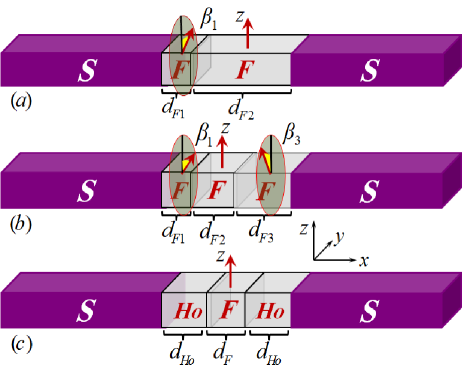
Figure 1: (Color online) Schematic of three experimental sets up. (a) simple $S$/$F$/$F$/$S$ Josephson junction with ferromagnetic layers’ widths $d_{F1}$, $d_{F2}$ and magnetization orientations $\vec{h}_{1}=h_{0}(0,\sin\beta_{1},\cos\beta_{1})$, $\vec{h}_{2}=h_{0}(0,0,1)$, respectively. (b) trilayer $S$/$F$/$F$/$F$/$S$ junction where the magnetization of middle $F$ layer, with width $d_{F2}$, is fixed in the $z$ direction. The other layers have $d_{F1}$, $d_{F3}$ widths with magnetization orientations $\vec{h}_{1,3}=h_{0}(0,\sin\beta_{1,3},\cos\beta_{1,3})$, respectively. (c) trilayer of ferromagnets where the outer $F$ layers have Holmium-like magnetization patterns namely, $\vec{h}_{Ho}=h_{0}(\cos\alpha,\sin\alpha\sin\gamma x/a,\sin\alpha\cos\gamma x/a)$. The length of middle $F$ layer is labeled by $d_{F}$ while the two outer Holmium-like $F$ layers are assumed to have equal lengths $d_{Ho}$. The $x$ axis is normal to the junction interfaces and the systems have infinite sizes in the $y$ and $z$ directions.

We consider weak exchange field strengths of $|\vec{h}|=5\Delta_{0}$ corresponding to that found in ferromagnet alloysZdravkov such as, e.g., ${\rm Cu}_{x}{\rm Ni}_{y}$. A barrier resistance of $\zeta=4.0$ ensures sufficiently opaque $S$/$F$ interfaces leading to appropriate solutions to the Usadel equations within the low proximity limit, $\underline{F}(x,y,z,\varepsilon)\ll\underline{1}$. Having now outlined the Keldysh-Usadel quasiclassical formalism and spin-parametrization framework employed in this work, we now proceed to present our analytical and numerical findings in the next sections.

III One-dimensional hybrid structures

In this section, we consider the effectively one-dimensional hybrid structures sketched in Fig. 1. We first derive the Usadel equations and boundary conditions. We then decompose the supercurrent into its singlet and triplet components using the three-dimensional spin-parametrization scheme discussed in Sec. II.2. Utilizing this singlet-triplet decomposition, we analyze and characterize the supercurrent behavior based on the individual components involved.

III.1 Spin-parameterized supercurrent

Upon decomposing the Green’s function via Eq. (11), the Usadel equation, Eq. (II.1), transforms into the following eight coupled complex partial differential equations for one-dimensional systems,

$$D\left\{\mp\partial_{x}^{2}\mathbb{T}_{x}(-\varepsilon)+i\partial_{x}^{2}\mathbb{T}_{y}(-\varepsilon)\right\}+i\left\{-2\varepsilon(\mp\mathbb{T}_{x}(-\varepsilon)+i\mathbb{T}_{y}(-\varepsilon))\mp 2\mathbb{S}(-\varepsilon)(h_{x}\mp ih_{y})\right\}=0$$ (12a)

$$D\left\{\mp\partial_{x}^{2}\mathbb{S}(-\varepsilon)+\partial_{x}^{2}\mathbb{T}_{z}(-\varepsilon)\right\}+i\left\{\mp 2\mathbb{T}_{x}(-\varepsilon)h_{x}\mp 2\mathbb{T}_{y}(-\varepsilon)h_{y}-2(\mp\mathbb{S}(-\varepsilon)+\mathbb{T}_{z}(-\varepsilon))(\varepsilon\pm h_{z})\right\}=0$$ (12b)

$$D\left\{\mp\partial_{x}^{2}\mathbb{T}_{x}^{\ast}(\varepsilon)-i\partial_{x}^{2}\mathbb{T}_{y}^{\ast}(\varepsilon)\right\}+i\left\{\pm 2(h_{x}\pm ih_{y})\mathbb{S}^{\ast}(\varepsilon)-2\varepsilon(\mp\mathbb{T}_{x}^{\ast}(\varepsilon)-i\mathbb{T}_{y}^{\ast}(\varepsilon))\right\}=0$$ (12c)

$$D\left\{\mp\partial_{x}^{2}\mathbb{S}^{\ast}(\varepsilon)+\partial_{x}^{2}\mathbb{T}_{z}^{\ast}(\varepsilon)\right\}+i\left\{2(-\varepsilon\pm h_{z})(\mp\mathbb{S}^{\ast}(\varepsilon)+\mathbb{T}_{z}^{\ast}(\varepsilon))\pm 2h_{x}\mathbb{T}_{x}^{\ast}(\varepsilon)\pm 2h_{y}\mathbb{T}_{y}^{\ast}(\varepsilon)\right\}=0$$ (12d)

The Kupriyanov-Lukichev boundary conditions at the left $S$/$F$ interface, Eq. (II.1), are transformed in the same way, leading to the following differential equations:

$$(\zeta\partial_{x}-c^{\ast}(\varepsilon))(\mp\mathbb{T}_{x}(-\varepsilon)+i\mathbb{T}_{y}(-\varepsilon))=0,$$ (13a)

$$(\zeta\partial_{x}-c^{\ast}(\varepsilon))(\mp\mathbb{S}(-\varepsilon)+\mathbb{T}_{z}(-\varepsilon))=\mp s^{\ast}(\varepsilon),$$ (13b)

$$(\zeta\partial_{x}-c^{\ast}(\varepsilon))(\mp\mathbb{T}_{x}^{\ast}(\varepsilon)-i\mathbb{T}_{y}^{\ast}(\varepsilon))=0,$$ (13c)

$$(\zeta\partial_{x}-c^{\ast}(\varepsilon))(\mp\mathbb{S}^{\ast}(\varepsilon)+\mathbb{T}_{z}^{\ast}(\varepsilon))=\pm s^{\ast}(\varepsilon).$$ (13d)

Similarly, the Kupriyanov-Lukichev boundary conditions at the right $F$/$S$ interface are also transformed as,

$$(\zeta\partial_{x}+c^{\ast}(\varepsilon))(\mp\mathbb{T}_{x}(-\varepsilon)+i\mathbb{T}_{y}(-\varepsilon))=0,$$ (14a)

$$(\zeta\partial_{x}+c^{\ast}(\varepsilon))(\mp\mathbb{S}(-\varepsilon)+\mathbb{T}_{z}(-\varepsilon))=\pm s^{\ast}(\varepsilon),$$ (14b)

$$(\zeta\partial_{x}+c^{\ast}(\varepsilon))(\mp\mathbb{T}_{x}^{\ast}(\varepsilon)-i\mathbb{T}_{y}^{\ast}(\varepsilon))=0,$$ (14c)

$$(\zeta\partial_{x}+c^{\ast}(\varepsilon))(\mp\mathbb{S}^{\ast}(\varepsilon)+\mathbb{T}_{z}^{\ast}(\varepsilon))=\mp s^{\ast}(\varepsilon).$$ (14d)

By solving this coupled set of complex differential equations with the boundary conditions [Eqs. (13) and (14)], the relevant physical quantities can be obtained. We consider the $x$-axis be normal to the interfaces, as shown in Fig. 5. The decomposition introduced above leads to the following expression for the supercurrent density within the junction [Eq. (8)]:

$$J(x)=J_{0}\int_{-\infty}^{\infty}d\varepsilon\left\{\right.$$

$$\left.\mathbb{S}(\varepsilon)\partial_{x}\mathbb{S}^{\ast}(-\varepsilon)-\mathbb{S}(-\varepsilon)\partial_{x}\mathbb{S}^{\ast}(\varepsilon)+\mathbb{S}(\varepsilon)^{\ast}\partial_{x}\mathbb{S}(-\varepsilon)-\right.$$

$$\left.\mathbb{S}(-\varepsilon)^{\ast}\partial_{x}\mathbb{S}(\varepsilon)-\partial_{x}\mathbb{T}_{x}(-\varepsilon)\mathbb{T}_{x}^{\ast}(\varepsilon)+\partial_{x}\mathbb{T}_{x}(\varepsilon)\mathbb{T}_{x}^{\ast}(-\varepsilon)-\right.$$

$$\left.\partial_{x}\mathbb{T}_{x}^{\ast}(-\varepsilon)\mathbb{T}_{x}(\varepsilon)+\partial_{x}\mathbb{T}_{x}^{\ast}(\varepsilon)\mathbb{T}_{x}(-\varepsilon)-\partial_{x}\mathbb{T}_{y}(-\varepsilon)\mathbb{T}_{y}^{\ast}(\varepsilon)+\right.$$

$$\left.\partial_{x}\mathbb{T}_{y}(\varepsilon)\mathbb{T}_{y}^{\ast}(-\varepsilon)-\partial_{x}\mathbb{T}_{y}^{\ast}(-\varepsilon)\mathbb{T}_{y}(\varepsilon)+\partial_{x}\mathbb{T}_{y}^{\ast}(\varepsilon)\mathbb{T}_{y}(-\varepsilon)-\right.$$

$$\left.\partial_{x}\mathbb{T}_{z}(-\varepsilon)\mathbb{T}_{z}^{\ast}(\varepsilon)+\partial_{x}\mathbb{T}_{z}(\varepsilon)\mathbb{T}_{z}^{\ast}(-\varepsilon)-\partial_{x}\mathbb{T}_{z}^{\ast}(-\varepsilon)\mathbb{T}_{z}(\varepsilon)+\right.$$

$$\left.\partial_{x}\mathbb{T}_{z}^{\ast}(\varepsilon)\mathbb{T}_{z}(-\varepsilon)\right\}\tanh(\varepsilon\beta).$$ (15)

The current through the junction can be easily obtained by integration of the current density along the $y$ and $z$ directions over the $F$ junction widths $W$ and $L$, respectively (corresponding to the cross section of the wire). We assume that our system is very wide in the $y$ direction, so that the one-dimensional approximation is valid, and therefore the current density remains constant in the $y$ and $z$ directions. It is convenient to define the normalization constant, $I_{0}\equiv LWJ_{0}$, for the supercurrent, $I(x)$. To extract the contributions to the total supercurrent from the even frequency singlet, and odd frequency triplet correlations, we have also decomposed the supercurrent accordingly into four components:

$$I_{S0}(x)=I_{0}\int_{-\infty}^{\infty}d\varepsilon\left\{\mathbb{S}(\varepsilon)\partial_{x}\mathbb{S}^{\ast}(-\varepsilon)-\mathbb{S}(-\varepsilon)\partial_{x}\mathbb{S}^{\ast}(\varepsilon)+\right.$$

$$\left.\mathbb{S}(\varepsilon)^{\ast}\partial_{x}\mathbb{S}(-\varepsilon)-\mathbb{S}(-\varepsilon)^{\ast}\partial_{x}\mathbb{S}(\varepsilon)\right\}\tanh(\varepsilon\beta),$$ (16a)

$$I_{Sx}(x)=I_{0}\int_{-\infty}^{\infty}d\varepsilon\left\{-\partial_{x}\mathbb{T}_{x}(-\varepsilon)\mathbb{T}_{x}^{\ast}(\varepsilon)+\partial_{x}\mathbb{T}_{x}(\varepsilon)\mathbb{T}_{x}^{\ast}(-\varepsilon)\right.$$

$$\left.-\partial_{x}\mathbb{T}_{x}^{\ast}(-\varepsilon)\mathbb{T}_{x}(\varepsilon)+\partial_{x}\mathbb{T}_{x}^{\ast}(\varepsilon)\mathbb{T}_{x}(-\varepsilon)\right\}\tanh(\varepsilon\beta),$$ (16b)

$$I_{Sy}(x)=I_{0}\int_{-\infty}^{\infty}d\varepsilon\left\{-\partial_{x}\mathbb{T}_{y}(-\varepsilon)\mathbb{T}_{y}^{\ast}(\varepsilon)+\partial_{x}\mathbb{T}_{y}(\varepsilon)\mathbb{T}_{y}^{\ast}(-\varepsilon)\right.$$

$$\left.-\partial_{x}\mathbb{T}_{y}^{\ast}(-\varepsilon)\mathbb{T}_{y}(\varepsilon)+\partial_{x}\mathbb{T}_{y}^{\ast}(\varepsilon)\mathbb{T}_{y}(-\varepsilon)\right\}\tanh(\varepsilon\beta),$$ (16c)

$$I_{Sz}(x)=I_{0}\int_{-\infty}^{\infty}d\varepsilon\left\{\partial_{x}\mathbb{T}_{z}(-\varepsilon)\mathbb{T}_{z}^{\ast}(\varepsilon)+\partial_{x}\mathbb{T}_{z}(\varepsilon)\mathbb{T}_{z}^{\ast}(-\varepsilon)\right.$$

$$\left.-\partial_{x}\mathbb{T}_{z}^{\ast}(-\varepsilon)\mathbb{T}_{z}(\varepsilon)+\partial_{x}\mathbb{T}_{z}^{\ast}(\varepsilon)\mathbb{T}_{z}(-\varepsilon)\right\}\tanh(\varepsilon\beta),$$ (16d)

where the total supercurrent is thus the sum of decomposed terms, namely,

$$I_{tot}(x)=I_{S0}(x)+I_{Sx}(x)+I_{Sy}(x)+I_{Sz}(x).$$ (17)

This decomposition allows for pinpointing the exact behavior of the even- and odd-frequency supercurrent components.

III.1.1 Results and discussions

Various analytical or numerical schemes with varying approximations have been employed to investigate the structures with magnetization patterns shown in Fig. 1 alidoust1 ; alidoust_missner ; alidoust2 ; Houzet3 ; Houzet1 ; rob2 ; Crouzy . In the analytical treatments Houzet3 ; robinson3 , limiting approximations were employed. For example, to study the noncollinear $S$/$F$/$F$/$F$/$S$ structures Houzet1 ; Houzet3 , transparent boundaries are employed at the $S$/$F$ interfaces together with the assumption that the anomalous Green’s function varies enough slowly through the magnetic trilayer to warrant its Taylor expansion. Our full numerical results involve no such approximations, and hence reveals cases where the inclusion of such effects may be important. One of the main aspects that our numerical approach reveals is the crucial role that each of the different types of superconducting correlations play in the total supercurrent, given by Eq. (8). The supercurrent is composed of different components of even-frequency singlet and odd-frequency triplet correlations $\mathbb{S}$, $\vec{\mathbb{T}}$, respectively. Such a decomposition is often neglected in Josephson structures that involve intricate magnetic textures.

For comparison purposes, we first consider the simpler $S/F/F/S$ heterostructureCrouzy shown in Fig. 1(a). Most of the results have $d_{F1}\neq d_{F2}$, and in all cases shown, the magnetization of the right $F$ layer is fixed along the $z$-axis while the left $F$ layer magnetization rotates in the $yz$ plane, that is, $\vec{h}_{1}=h_{0}(0,\sin\beta_{1},\cos\beta_{1})$. The magnetization orientation of the left $F$ is thus characterized by the angle $\beta_{1}$, since the magnetization is entirely in-plane.

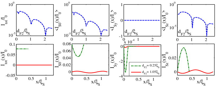
Figure 2: (Color online) Top row: Critical supercurrent and its components as a function of $d_{F2}$, the width of the right magnetic layer in a $S/F/F/S$ junction (see Fig. 1(a)). The width of the first magnetic layer is fixed at $d_{F1}=0.15\xi_{S}$. The current components are calculated by performing a spatial average over the right $F$ layer ($\langle I_{S0}(x)/I_{0}\rangle,\langle I_{Sy}(x)/I_{0}\rangle,\langle I_{Sz}(x)/I_{0}\rangle$). Bottom row: Spatial behavior of the critical Josephson current and its components as a function of position $x$ inside the junction for two typical values of $d_{F2}=0.25\xi_{S}$, and $d=1.05\xi_{S}$. The magnetization orientation in the left $F$ layer is fixed at a representative value of $\beta_{1}=0.2\pi$, while the magnetization in the right $F$ layer always points along $z$, corresponding to $\beta_{2}=0$.

The top row of Fig. 2 illustrates the total critical supercurrent $I_{tot}$ and its decomposed components ($I_{S0}$, $I_{Sx}$, $I_{Sy}$, $I_{Sz}$) versus the thickness of right $F$ layer, $d_{F2}$. The current components generally vary with position $x$, so in order to display an overall view of their behavior as a function of magnetization orientation, we spatially average [denoted by $\langle...\rangle$] each component over $d_{F2}$. The thickness of the left $F$ layer is set typically at $d_{F1}=0.15\xi_{S}$, and its magnetization has two components $h_{y}$, and $h_{z}$, using a representative angle of $\beta_{1}=0.2\pi$ (these values are chosen to in part support our comparison purposes in Subsec. IV.6). To show the fine features of the $0$-$\pi$ transition profiles, we have used a logarithmic scale for the magnitude of the critical supercurrent and its decomposed components. The critical current (far left panel) undergoes multiple $0$-$\pi$ transitions when varying $d_{F2}$. The decomposed current components $\langle I_{S0}\rangle$ and $\langle I_{Sz}\rangle$ also show the same behavior as seen in the remaining panels. Next, in the bottom row of Fig. 2, we plot the maximum current and its components as a function of position for two representative values of the right $F$ layer’s thickness ($d_{F2}=0.25\xi_{S}$, and $d_{F2}=1.05\xi_{S}$). The current components, in contrast to the total current, often vary inside the magnetic layers: $I_{S0}$, and $I_{Sz}$ are shown to propagate within the two $F$ layers. The spin-1 triplet component, $I_{Sy}$, is however localized within the left $F$ layer where $\beta_{2}=0.2\pi$ and thus $h_{y}\neq 0$. We have investigated a wide range of parameter sets, involving $\beta_{1}$, $d_{F1}$, and the superconducting phase differences. The $I_{Sy}$ component, does not propagate into the right $F$ region where the exchange field is directed along $z$, demonstrating consistency with previous studiesHouzet1 . As discussed in the introduction, recent theoretical works showed that signatures of the triplet supercurrent may be detected by the appearance of a second harmonic in the supercurrent in ballistic $S/F/F/S$ Josephson junction, provided that $d_{F1}\gg d_{F2}$. The higher harmonics were shown to decay exponentially (faster than the first harmonic) when varying the system parameters such as the thickness of the magnetic layers, and exchange field intensities, in the full proximity limit of the diffusive regime.buzdin1 Therefore, in the low proximity limit we consider in our manuscript, the higher harmonics are absent.buzdin1 It has been suggested that a trilayerHouzet1 ; Houzet3 of uniform magnetic materials with noncollinear magnetizations can reveal the signatures of long-ranged spin-triplet correlations where the two outer layers produce nonzero spin projections which can be detected in the middle $F$ layer with orthogonal magnetization. To elucidate the source of the long-range triplet behavior in these types of trilayer configurationsHouzet3 , we investigate next the details of the individual components comprising the total supercurrent.

We therefore consider a $S$/$F$/$F$/$F$/$S$ trilayer structure, as depicted in Fig. 1(b). The magnetization of the central $F$ layer is pinned in the $z$ orientation, coinciding with the spin-quantization axis. The relative in-plane magnetization directions in the surrounding left and right $F$ layers are described simply by the angles $\beta_{1}$, and $\beta_{2}$, respectively. We denote the thicknesses of the left, middle, and right $F$ layers by $d_{F1}$, $d_{F2}$, and $d_{F3}$, respectively. In the top set of

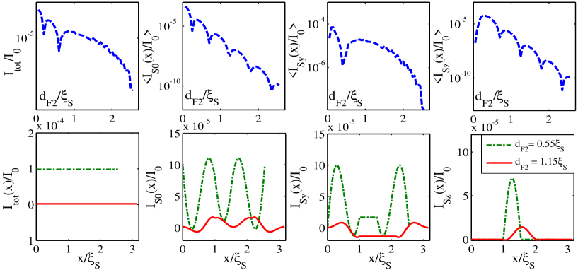
Figure 3: (Color online) Top row: Critical supercurrent and its components against the thickness of the middle $F$ layer $d_{F2}$ in the $S/F/F/F/S$ structure shown in Fig. 1(b). The thickness of the outer $F$ layers, $d_{F1}$ and $d_{F3}$, are equal and fixed at $\xi_{S}$. The components are spatially averaged over the middle $F$ layer thickness ($\langle I_{S0}(x)/I_{0}\rangle,\langle I_{Sy}(x)/I_{0}\rangle,\langle I_{Sz}(x)/I_{0}\rangle$). Bottom row: Critical current as a function of position inside the junction $x$ for two different thicknesses of the middle $F$ layer, $d_{F2}=0.55\xi_{S}$, and $d_{F2}=1.15\xi_{S}$. The magnetization of the middle $F$ layer is fixed along the $z$ direction, $\beta_{2}=0$, while the magnetization is oriented towards the $y$ direction in the outer $F$ layers ($\beta_{1}=\beta_{3}=\pi/2$).

panels in Fig. 3, the spatially averaged supercurrent and its singlet and triplet constituents are shown as a function of $d_{F2}$. We here show the results for $d_{F1}=d_{F3}=\xi_{S}$, which is representative of the numerous equal-width cases investigated numerically. The bottom set of panels illustrate the spatial behavior of the supercurrent and its components. To isolate the spin-1 triplet contribution, $I_{Sy}$, to the supercurrent in the middle $F$ layer, we set $\beta_{1}=\beta_{3}=\pi/2$. In this case, the magnetization of the two outer $F$ layers are strictly along $y$ and orthogonal to the exchange field direction of middle $F$. Such a magnetization configuration has been suggested as optimal for detecting the signatures of the spin triplet supercurrents Houzet3 . As seen in the figure, the critical supercurrent versus the middle $F$ layer thickness shows multiple $0$-$\pi$ transitions, corresponding to points where the current nearly vanishes and then eventually changes sign. The averaged components of the total supercurrent, $I_{S0}$ and $I_{Sz}$ demonstrate short-range signatures as exhibited by the multiple cusps compared to the equal-spin triplet component $I_{Sy}$. The total critical current behavior is dominated by the triplet term, $I_{Sy}$, which undergoes fewer sign changes than the other components, and consequently fewer $0$-$\pi$ transitions, when changing $d_{F2}$. Thus for the regime considered here, the supercurrent does not exhibit a very slow monotonic decay as a function of the central magnetic junction thickness, as reflected in the absence of long-ranged behavior in $I_{Sy}$ vs $d_{F2}$.

To further explore the behavior of the current throughout the junction, we next examine (bottom row, Fig. 3) the spatial dependence to the total supercurrent and its singlet and triplet components for representative values of unequal middle $F$ layer thicknesses, $d_{F2}=0.55\xi_{S}$, and $d_{F2}=1.15\xi_{S}$. We immediately observe from the left panel that as expected, the maximum total supercurrent is a constant in all parts of the junction, reflecting conservation of current there. The triplet component with zero-spin projection, $I_{Sz}$, is localized in the middle $F$ layer where the magnetization is directed along $z$. In contrast, the singlet component $I_{S0}$ oscillates throughout the junction while the triplet component, $I_{Sy}$, propagates without decay in the middle ferromagnet, which has its magnetization direction orthogonal to the spin orientation of $I_{Sy}$. Thus, we observe that $I_{Sy}$ is long-ranged in the middle $F$ layer. Although $I_{Sy}$ is spatially constant throughout the middle $F$ layer, it changes sign, depending on $d_{F2}$. This characteristic is seen in the top row of Fig. 3. We have investigated with our full numerical method several different geometrical parameter sets, including, e.g., much smaller $d_{F1}$, and $d_{F3}$, as well as other $\beta_{1}$, and $\beta_{3}$. We typically found that the results presented in the top row of Fig. 3 are quite representative of the singlet and triplet supercurrent behavior for the low proximity regime.

In a recent experimentrob1 involving $Ho/F/Ho$ trilayers with inhomogeneous magnetization patterns, a long-ranged Josephson supercurrent through the ferromagnet was detected. We here fully characterize the long-ranged triplet correlations in such $S/Ho/F/Ho/S$ Josephson junctions (see Fig. 1(c)). The sandwiched central $F$ layer represents a material with uniform magnetization, e.g., Cobalt, while the outer two $Ho$ layers represent ferromagnets with a conical magnetization texture, such as that found in Holmium ($Ho$). As with the previous structures, we focus the study on the supercurrent behavior as a function of the central $F$ layer thickness. We find that the supercurrent decays uniformly without any sign change when varying the middle $F$ layer thickness, in agreement with other worksrob2 . However, the precise underlying role of the singlet and triplet components in the overall supercurrent behavior has been lacking.

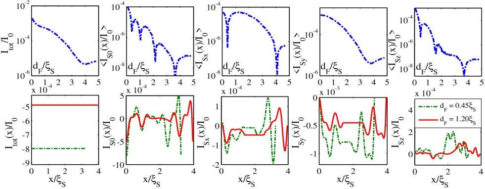
Figure 4: (Color online) Top row: Critical current and its components versus middle $F$ layer thickness, $d_{F}$ in $S/Ho/F/Ho/S$ structure where the outer $F$ layers’ magnetization pattern is Holmium ($Ho$)-like . The configuration is illustrated schematically in Fig. 1(c). The thicknesses of the outer $F$ layers are fixed at $d_{Ho}=1.4\xi_{S}$, whereas the magnetization is fixed along the $z$ direction in the middle $F$ layer, $\beta_{2}=0$. The components of the critical supercurrents are calculated by spatially averaging over the thickness of the middle $F$ layer ($\langle I_{S0}(x)/I_{0}\rangle,\langle I_{Sy}(x)/I_{0}\rangle,\langle I_{Sz}(x)/I_{0}\rangle$). Bottom row: Critical supercurrent against position inside the magnetic junction $x$ where the thickness of middle $F$ layer has two values $d_{F}=0.45\xi_{S},1.2\xi_{S}$.

In Fig. 4, we exhibit the total current and its decomposition for a variety of parameters appropriate for the inhomogeneous conical magnetic junction. The middle $F$ layer is magnetized along $z$, while the conical magnetization patterns of the Holmium layers have the adopted form:

$$\vec{h}_{Ho}=h_{0}\left(\cos\alpha,\sin\alpha\sin(\gamma x/a),\sin\alpha\cos(\gamma x/a)\right),$$ (18)

with the following material parameters: $a=0.02d$ is the distance of interatomic layers, $d$ denotes the junction thickness, $\alpha=4\pi/9$ is the apex angle, and $\gamma=\pi/6$ is the rotation angle of the cone structure, consistent with experimental values Sosnin . The magnitude of the exchange field is unchanged throughout the $F$ regions. The top set of panels in Fig. 4 shows the critical total current and its components as a function of the middle uniform $F$ layer thickness $d_{F}$. The components $I_{S0}$, $I_{Sy}$, and $I_{Sz}$ are averaged over the middle $F$ layer [denoted by $\langle...\rangle$]. We assume the two $Ho$ layers have identical magnetization patterns rob2 , and both thicknesses equal $d_{Ho}=1.4\xi_{S}$. The first panel on the left shows the total critical supercurrent versus $d_{F}$ and exhibits the expected decay over a few coherence lengths. Examining the signatures of the other components in the top panels, we see that the opposite-spin singlet and triplet components, $I_{S0}$ and $I_{Sz}$ respectively, demonstrate well defined oscillatory behavior and corresponding sign changes as a function of $d_{F}$. We can also conclude that the net supercurrent arises mainly from the spin-1 projection of the triplet components, $I_{Sy}$, which is long-ranged in the middle $F$ with an exchange field direction orthogonal to the spin-orientation of $I_{Sy}$. For the Holmium magnetization profile, $h_{x}$ does not vary in space, and therefore $I_{Sx}$ behaves similarly to the $I_{Sy}$ component in the $S/F/F/F/S$ structure (see Fig. 3). Although $I_{Sx}$ undergoes fewer sign changes when varying $d_{F}$, the $0$-$\pi$ transitions are clearly present for this component. The triplet component, $I_{Sy}$, the main contributor to the total current, does not switch directions when increasing the middle $F$ layer thickness $d_{F}$, and its magnitude often dominates the other components. Its nearly monotonic decay can be traced back to the corresponding component of the magnetization profile: in the $Ho$ layer, $h_{y}$ rotates sinusoidally as a function of position, generating long-ranged odd-frequency correlations that are not subject to the spin-splitting effects of the magnet responsible also for the oscillatory behavior of superconducting correlations. We have also found consistency with previous studiesrob2 , where the monotonic decay of the supercurrent appears when $d_{Ho}$ is large enough to contain at least one spiral period. On the other hand, the sign changing behavior emerges for small $d_{Ho}$, so that the $Ho$ layers effectively mimics a uniform ferromagnet. This aspect was revisited in a recent work employing a lattice model.annett The bottom row of Fig. 4 illustrates the decomposed components of the maximum total supercurrent as a function of position throughout the ferromagnet regions. Two representative thicknesses of the middle $F$ layer are considered: $d_{F}=0.4\xi_{S}$, and $d_{F}=1.2\xi_{S}$. Similar to the $S/F/F/F/S$ junction above, the triplet components with spin projection $m=\pm 1$ on the $z$-axis ($I_{Sx}$ and $I_{Sy}$), are constant over the entire middle $F$ region and therefore can be classified as long-ranged. To summarize this section, we studied the behavior of the critical supercurrent through low-proximity one-dimensional structures shown in Fig. 1. By directly decomposing the supercurrent using the spin-parametrization technique given in the theoretical methods section, we numerically studied the origins of the supercurrent behavior in terms of its short-ranged and long-ranged components. Our results showed that $S$/$F$/$F$/$S$ structures do not support any long-ranged supercurrent components, reaffirming the findings of Ref. Houzet1, , while $S$/$F$/$F$/$F$/$S$ junctions host long-ranged supercurrent componentsHouzet3 that are more prominent in the inhomogeneous $S$/$Ho$/$F$/$Ho$/$S$ structures as experimentally observed in Ref. rob1, and verified theoretically by numerical studied of full proximity regime in Ref. rob2, . We showed that the long-ranged supercurrent component corresponds to the rotating component of the magnetization texture, and is the main contributor to the total supercurrent. The numerical results presented in this section shall be used for later comparisons when we categorize structures into two classes based on the supercurrent direction with respect to the $F$/$F$ interface orientation: parallel or perpendicular. The one-dimensional structures in Fig. 1 belong to the latter class. We now direct our attention to two-dimensional hybrids, including the possibility of an applied magnetic field. The singlet-triplet decompositions discussed above shall be employed to pinpoint exactly the spatial behavior of the associated components of the total charge supercurrent.

IV two-dimensional hybrid structures

In this section we present the main results of the paper. We first consider a two-dimensional magnetic $S$/$F$/$S$ system subject to an external magnetic field for two regimes: the wide junction $W_{F}$ $\gg$ $d_{F}$, and the narrow junction $W_{F}$ $\ll$ $d_{F}$ regimes. The magnetic strips are sandwiched between two $s$-wave superconducting reservoirs, where the exchange field in the $F$ strips is spatially uniform. This permits analytical solutions that are capable of accurately predicting the behavior of relevant physical quantities such as charge and spin supercurrents, as well as the pair potential. The analytical results are complemented with full numerical investigations, including studies of the dependence of the critical charge supercurrent on the external magnetic field, and the corresponding appearance of proximity vortices. The current density spatial map is also investigated, giving a global view of the distribution of supercurrents throughout the junction. We next consider two kinds of finite-sized magnetic $S$/$F$/$F$/$S$ Josephson junctions subject to an external magnetic field. For these systems, analytical routes are scarce, and we must in general resort to numerical approaches. In one case, we assume the double layer magnetic $F$ strips comprising the $F$/$F$ junction are parallel with the $S$ interfaces. In the other case, however, we assume that the $F$ strips are perpendicular to the $S$ interfaces. Using the spin-parametrization introduced in Sec. II.2, we can then study the even and odd frequency components of the total charge Josephson current inside the proposed structures.

IV.1 Technical assumptions and parameters

In this subsection, we discuss the assumptions used in our calculations, along with the parameters and notations used throughout. As was previously mentioned, the external magnetic field is confined within the non-superconducting regionsCuevas_frh2 ; Cuevas_frh1 ; alidoust_nfrh1 (see Fig. 5). We restrict the magnetic field to be oriented perpendicular to the junction plane, which for our coordinate system corresponds to the $z$-axis. Thus, supercurrent flow resides in the $xy$ plane. The situation where the external magnetic field is parallel to the current direction has been studied both experimentally and theoretically.Birge We can therefore represent the magnetic field as, $\vec{H}(x)=\vec{H}\Theta(x)\Theta(d_{F}-x)$, where $d_{F}$ is the junction length and $\vec{H}=(0,0,H_{z})$. This assumption also ensures that the macroscopic phases of the two superconducting electrodes are unaffected by the external magnetic field. This widely used assumption has demonstrated good qualitative agreement with experimental measurements. Cuevas_frh1 ; Cuevas_frh2 ; alidoust_nfrh1 ; Angers

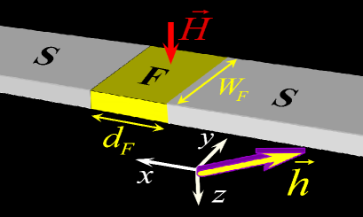
Figure 5: Proposed setup of the Josephson $S$/$F$/$S$ junction subject to an external magnetic field $\vec{H}$. The magnetic wire ($F$) with rectangular dimensions, $d_{F}$ and $W_{F}$, is sandwiched between two $s$-wave superconducting ($S$) leads. The exchange field of the magnetic layer, $\vec{h}=(h^{x},h^{y},h^{z})$, can take arbitrary orientations. The external magnetic field is oriented along the $z$ direction. The two-dimensional system resides in the $xy$ plane so that the interfaces are along the $y$ direction and $x$ axis is normal to the junction.

The Josephson junctions investigated in this work therefore are assumed to have negligible magnetic field screening.Angers ; Chiodi If on the contrary, the magnetic field is not restricted to the $F$ regions, it becomes necessary to solve a set of partial differential equations, Eq. (II.1), self-consistently in tandem with Maxwell’s equations and the superconducting order parameter $\Delta(x,y,T)$. Hence, a suitable choice for the vector potential $\vec{A}$ that we use satisfying the Coulomb gauge, $\vec{\nabla}\cdot\vec{A}=0$, is, $\vec{A}(x)=(-yH_{z}(x),0,0)$. In normalizing our equations, we write the external magnetic flux as $\Phi=\tilde{\Phi}/\Phi_{0}$, where $\tilde{\Phi}\equiv W_{F}d_{F}H_{z}$, $W_{F}$ is the junction width, and $\Phi_{0}=\hbar/2e$ is the magnetic flux quantum.

IV.2 Uniform $S$/$F$/$S$ heterostructures

We here consider a two-dimensional ferromagnetic $S$/$F$/$S$ Josephson junction where the magnetization of the magnetic strip is homogeneous. Although our theoretical approach allows for completely general patterns in the magnetization texture, we restrict our focus here to a specific case where the exchange field has only one component along the $z$ direction, $\vec{h}(x,y,z)=(0,0,h^{z})$, thus permitting analytical solutions to the Usadel equation. The two-dimensional junction resides in the $xy$ plane so that the $S$/$F$ interfaces are parallel with the $y$ axis (see Fig. 5). The corresponding system of coupled partial differential equations [Eq. (II.1)], now reduces to a smaller set of decoupled partial differential equations. We are then able to derive analytical expressions for the anomalous component of the Green’s function and therefore the charge supercurrent and pair potential.

Using this simplified system of decoupled partial differential equations, we consider two regimes: In the first case, we assume the junction width $W_{F}\gg d_{F}$, thus, terms involving the ratio $d_{F}/W_{F}$ can be dropped, leading to further simplifications. In the second regime, the junction width $W_{F}\ll d_{F}$, corresponding to a narrow magnetic nanowire. To be complete, we also implement a full numerical investigation, without the simplifying assumptions above and with arbitrary values of ratio $W_{F}/d_{F}$. This requires numerical solutions to a complex system of partial differential equations [see Eqs. (II.1)]. Several checks on the numerics were performed, including reproducing previous results involving nonmagnetic $S$/$N$/$S$ Josephson junctions, where the exchange field of the $F$ layer is equal to zero.Cuevas_frh1 ; Cuevas_frh2

The full Usadel equations in the presence of an external magnetic field $\vec{H}$, and corresponding vector potential, $\vec{A}$, are written:

$$\vec{\nabla}^{2}f_{\pm}(-\varepsilon)-2ie\vec{\nabla}\cdot\vec{A}f_{\pm}(-\varepsilon)-4ie\vec{A}\cdot\vec{\nabla}f_{\pm}(-\varepsilon)-$$

$$4e^{2}A^{2}f_{\pm}(-\varepsilon)-\frac{2i(\varepsilon\mp h^{z})}{D}f^{R}_{\pm}(-\varepsilon)=0,$$ (19a)

$$\vec{\nabla}^{2}f^{*}_{\pm}(\varepsilon)+2ie\vec{\nabla}\cdot\vec{A}f^{*}_{\pm}(\varepsilon)+4ie\vec{A}\cdot\vec{\nabla}f^{*}_{\pm}(\varepsilon)-$$

$$4e^{2}A^{2}f^{*}_{\pm}(\varepsilon)-\frac{2i(\varepsilon\pm h^{z})}{D}f^{*}_{\pm}(\varepsilon)=0,$$ (19b)

where $\vec{\nabla}\equiv(\partial_{x},\partial_{y},\partial_{z})$. The above decoupled partial differential equations appear only for a magnetic junction where the magnetization has one component $\vec{h}=(0,0,h^{z})$. If we now expand the boundary conditions given by Eq. (II.1), at the left $S$/$F$ interface, we find,

$$\Big{\{}\zeta(\vec{\nabla}-2ie\vec{A})-c^{\ast}(\varepsilon)\pm i\frac{G_{S}}{G_{T}}\Big{\}}f_{\mp}(-\varepsilon)=\mp s^{\ast}(\varepsilon)e^{-i\theta_{l}},$$ (20a)

$$\Big{\{}\zeta(\vec{\nabla}+2ie\vec{A})-c^{\ast}(\varepsilon)\mp i\frac{G_{S}}{G_{T}}\Big{\}}f^{\ast}_{\mp}(\varepsilon)=\pm s^{\ast}(\varepsilon)e^{i\theta_{l}},$$ (20b)

while the boundary conditions at the right interface take the following form:

$$\Big{\{}\zeta(\vec{\nabla}-2ie\vec{A})+c^{\ast}(\varepsilon)\mp i\frac{G_{S}}{G_{T}}\Big{\}}f_{\mp}(-\varepsilon)=\pm s^{\ast}(\varepsilon)e^{-i\theta_{r}},$$ (21a)

$$\Big{\{}\zeta(\vec{\nabla}+2ie\vec{A})+c^{\ast}(\varepsilon)\pm i\frac{G_{S}}{G_{T}}\Big{\}}f^{\ast}_{\mp}(\varepsilon)=\mp s^{\ast}(\varepsilon)e^{i\theta_{r}}.$$ (21b)

The simplifying geometric approximations mentioned above can now be applied to the above equations, while adhering to the requirement that the corresponding regimes are experimentally accessible.

IV.2.1 Wide junction limit, $W_{F}$ $\gg$ $d_{F}$: Analytical results

If we assume that the width of junction is much larger than its length, terms involving $d_{F}/W_{F}$ in Eq. (19) can be neglected, yielding the following decoupled Usadel equations:

$$\partial^{2}_{x}f_{\pm}(-\varepsilon)+4i\Phi y\partial_{x}f_{\pm}(-\varepsilon)-4\Phi^{2}y^{2}f_{\pm}(-\varepsilon)$$

$$-2i\frac{\epsilon_{\mp}}{\epsilon_{T}}f_{\pm}(-\varepsilon)=0,$$ (22a)

$$\partial^{2}_{x}f^{\ast}_{\pm}(\varepsilon)+4i\Phi y\partial_{x}f^{\ast}_{\pm}(\varepsilon)-4\Phi^{2}y^{2}f^{{}^{\ast}}_{\pm}(\varepsilon)$$

$$-2i\frac{\epsilon_{\pm}}{\epsilon_{T}}f^{{}^{\ast}}_{\pm}(\varepsilon)=0.$$ (22b)

Here, we define $\epsilon_{\pm}\equiv\varepsilon\pm h^{z}(x,y,z)$, and the Thouless energy $\epsilon_{T}=D/d_{F}^{2}$. Note that all partial derivatives in Eqs. (22) are solely with respect to the $x$ coordinate. In other words, the original two-dimensional problem is now reduced to a quasi one-dimensional one. These uncoupled differential equations can be solved analytically thus permitting additional insight into the transport properties of ferromagnetic Josephson junctions. The Kupriyanov-Lukichev boundary conditions, Eq. (II.1), at the left $S$/$F$ interface located at $x=0$ reduces to:

$$\Big{\{}\zeta(\partial_{x}+2iy\Phi)+c(-\varepsilon)\mp i\frac{G_{S}}{G_{T}}\Big{\}}f_{\pm}(-\varepsilon)=\mp s(-\varepsilon)e^{i\theta_{l}},$$ (23a)

$$\Big{\{}\zeta(\partial_{x}-2iy\Phi)+c(-\varepsilon)\pm i\frac{G_{S}}{G_{T}}\Big{\}}f^{\ast}_{\pm}(\varepsilon)=\pm s(-\varepsilon)e^{-i\theta_{l}}.$$ (23b)

Similarly, the boundary conditions at the right $S$/$F$ interface located at $x=d_{F}$ can be written as follows:

$$\Big{\{}\zeta(\partial_{x}+2iy\Phi)-c(-\varepsilon)\pm i\frac{G_{S}}{G_{T}}\Big{\}}f_{\pm}(-\varepsilon)=\pm s(-\varepsilon)e^{-i\theta_{r}},$$ (24a)

$$\Big{\{}\zeta(\partial_{x}-2iy\Phi)-c(-\varepsilon)\mp i\frac{G_{S}}{G_{T}}\Big{\}}f^{\ast}_{\pm}(\varepsilon)=\mp s(-\varepsilon)e^{i\theta_{r}}.$$ (24b)

The macroscopic phases of the left and right superconducting terminals are labeled $\theta_{l}$ and $\theta_{r}$, respectively. The magnetic strips are assumed isolated in the $y$ direction so that physically no current passes through the boundaries at $y=0$, and $y=W_{F}$. Thus, to ensure that the supercurrent does not pass through the vacuum boundaries in the $y$ direction, we have the following conditions:

$$\partial_{y}f_{\pm}(\pm\varepsilon)=0,$$ (25a)

$$\partial_{y}f^{\ast}_{\pm}(\pm\varepsilon)=0.$$ (25b)

With the solutions to Eq. (22) at hand, we are now in a position to calculate the current density and the pair potential for a given magnetic flux. The current density, given by Eq. (8), can thus be expressed as:

$$\vec{J}(x,y)=J_{0}\int_{-\infty}^{\infty}d\varepsilon\tanh(\varepsilon\beta)\Big{\{}\Big{.}f_{-}(-\varepsilon)\vec{\nabla}f^{*}_{+}(\varepsilon)$$

$$+f_{+}(-\varepsilon)\vec{\nabla}f^{*}_{-}(\varepsilon)-f_{+}(\varepsilon)\vec{\nabla}f^{*}_{-}(-\varepsilon)-f_{-}(\varepsilon)$$

$$\vec{\nabla}f^{*}_{+}(-\varepsilon)+f^{*}_{-}(-\varepsilon)\vec{\nabla}f_{+}(\varepsilon)+f^{*}_{+}(-\varepsilon)\vec{\nabla}f_{-}(\varepsilon)$$

$$-f^{*}_{+}(\varepsilon)\vec{\nabla}f_{-}(-\varepsilon)-f^{*}_{-}(\varepsilon)\vec{\nabla}f_{+}(-\varepsilon)+4ie\vec{A}\big{[}\Big{.}$$

$$f^{*}_{-}(\varepsilon)f_{+}(-\varepsilon)-f^{*}_{+}(-\varepsilon)f_{-}(\varepsilon)-f^{*}_{-}(-\varepsilon)f_{+}(\varepsilon)$$

$$\big{.}+f^{*}_{+}(\varepsilon)f_{-}(-\varepsilon)\big{]}\Big{\}}.$$ (26)

The normalized pair potential, Eq. (10) now reads:

$$\tilde{U}_{\text{pair}}=\int_{-\infty}^{\infty}\big{[}f_{+}(\varepsilon)-f_{+}(-\varepsilon)+\big{.}$$

$$\big{.}f_{-}(-\varepsilon)-f_{-}(\varepsilon)\big{]}\tanh(\varepsilon\beta)d\varepsilon.$$ (27)

If we solve the Usadel equations Eqs. (22) using the boundary conditions (23) and (25), we arrive at the following solutions to the anomalous component of the Green’s function:

$$f_{\pm}(-\varepsilon)=\mp\frac{\mathcal{N}^{\pm}}{\mathcal{D}^{\pm}},$$ (28)

where the numerators $\mathcal{N}^{\pm}$ and denominators $\mathcal{D}^{\pm}$ are given by

$$\mathcal{N}^{\pm}=s^{\ast}(\varepsilon)e^{-\frac{1}{2}i(4xy\Phi+\phi)}\Big{\{}e^{2iy\Phi}\big{[}\zeta\lambda_{\mp}\cosh(x\lambda_{\mp})+\Big{.}\big{.}$$

$$\big{(}c^{\ast}(\varepsilon)\pm i\frac{G_{S}}{G_{T}}\big{)}\sinh(x\lambda_{\mp})\big{]}+e^{i\phi}\big{[}\zeta\lambda_{\mp}\times\big{.}$$

$$\Big{.}\big{.}\cosh(\lambda_{\mp}-x\lambda_{\mp})+\big{(}c^{\ast}(\varepsilon)\pm i\frac{G_{S}}{G_{T}}\big{)}\sinh(\lambda_{\mp}-x\lambda_{\mp})\big{]}\Big{\}},$$

$$\mathcal{D}^{\pm}=\sinh(\lambda_{\mp})\Big{\{}\zeta^{2}\lambda_{\mp}^{2}+\big{(}c^{\ast}(\varepsilon)\pm i\frac{G_{S}}{G_{T}}\big{)}^{2}\Big{\}}+$$

$$2\zeta\lambda_{\mp}\big{(}c^{\ast}(\varepsilon)\pm i\frac{G_{S}}{G_{T}}\big{)}\cosh(\lambda_{\mp}).$$

Similar solutions can be found for $f^{*}_{\pm}(-\varepsilon)$. In order to simplify notation, we have defined $\lambda_{\pm}=2i(\epsilon\pm h^{z})/\epsilon_{T}$, and the macroscopic phase difference of the superconducting terminals is denoted by $\phi=\theta_{l}-\theta_{r}$. The charge current density expressed by Eq. (IV.2.1) involves eight terms, $f_{\pm}(\pm\varepsilon)$, and $f_{\pm}^{\ast}(\pm\varepsilon)$, which should be derived to obtain an analytical expression for the supercurrent flow. In our calculations thus far, the interfaces are assumed spin-active, namely, $G_{S}/G_{T}\neq 0$. To maintain tractable analytic solutions, we drop the $c(\varepsilon)$-terms in addition to the spin-active contributions, which is appropriate for experimental conditions involving highly impure superconducting terminals. These widely used approximations lead to intuitive and physically relevant analytical solutions.bergeret1 ; buzdin1 ; alidoust2 Substituting the solutions to the Usadel equations into Eq. (IV.2.1), we find the charge supercurrent density in the $x$ direction:

$$I(\phi)=J_{0}\int_{-\infty}^{\infty}d\varepsilon\frac{2i\tanh(\varepsilon\beta)\mathbb{N}}{\zeta^{2}\lambda_{-}\lambda_{+}}\int_{-1/2}^{1/2}dy\sin(\phi-2y\Phi),$$ (29)

where,

$$\mathbb{N}={s^{\ast}}^{2}(-\varepsilon)\Big{(}\lambda_{+}\csc(\lambda_{-})+\lambda_{-}\csc(\lambda_{+})\Big{)}+$$

$${s^{\ast}}^{2}(\varepsilon)\Big{(}\lambda_{+}\text{csch}(\lambda_{-})+\lambda_{-}\text{csch}(\lambda_{+})\Big{)}.$$

Integrating the junction width over the $y$-direction, we end up with the total charge supercurrent across the junction:

$$I(\phi,\Phi)=I_{0}\sin\phi\frac{\sin\Phi}{\Phi},$$ (30)

where we have extracted the phase and flux dependent terms and absorbed the remaining coefficients into $I_{0}$. The maximum charge supercurrent occurs when the superconducting phase difference equals $|\phi|=\pi/2$. From Eq. (30), we see immediately that the critical charge current exhibits the well-known Fraunhofer interference diffraction pattern as a function of the externally applied flux $\Phi$. We also recover the results of a normal $S$/$N$/$S$ junction Cuevas_frh2 , where $h^{z}=0$. Thus, our analytical expressions for wide $S$/$F$/$S$ Josephson junctions experiencing perpendicularly directed external magnetic flux yields the same critical current response as a normal $S$/$N$/$S$ junctionCuevas_frh2 ). Here, however, there are additional, experimentally tunable physical quantities which can cause sign changes in $I_{0}(h^{z},G_{S}/G_{T})$, and consequently $I(\phi,\Phi)$. When presenting a global view of the current density, it is illustrative to examine a spatial map of its behavior. By utilizing Eq. (8), it is possible to calculate the charge current density throughout the $xy$ plane for a wide magnetic $S$/$F$/$S$ Josephson junction.

If we now insert the recently obtained solutions to the Usadel equations into the pair potential equation, Eq. (IV.2.1), we arrive at the following analytical formula which provides a spatial map of $U_{\text{pair}}$ for a wide junction:

$$\tilde{U}_{\text{pair}}=\int_{-\infty}^{+\infty}d\varepsilon\Big{\{}e^{-\frac{i}{2}(\phi+4xy\Phi)}\big{(}\big{[}s^{\ast}(-\varepsilon)\lambda_{+}\cos(x\lambda_{-})\times\big{.}\big{.}\Big{.}$$

$$\csc(\lambda_{-})+s^{\ast}(-\varepsilon)\lambda_{-}\cos(x\lambda_{+})\csc(\lambda_{+})+s^{\ast}(\varepsilon)\lambda_{+}\times$$

$$\cosh(x\lambda_{-})\text{csch}(\lambda_{-})+s^{\ast}(\varepsilon)\lambda_{+}\cosh(x\lambda_{+})\text{csch}(\lambda_{+})\big{]}e^{2iy\Phi}$$

$$+\big{[}s^{\ast}(-\varepsilon)\lambda_{+}\cos(\lambda_{-}-x\lambda_{-})\csc(\lambda_{-})+s^{\ast}(-\varepsilon)\lambda_{-}\times\big{.}$$

$$\cos(\lambda_{+}-x\lambda_{+})\csc(\lambda_{+})+s^{\ast}(\varepsilon)\lambda_{+}\cosh(\lambda_{-}-x\lambda_{-})\times$$

$$\big{.}\big{.}\Big{.}\text{csch}(\lambda_{-})+s^{\ast}(\varepsilon)\lambda_{-}\cosh(\lambda_{+}-x\lambda_{+})\text{csch}(\lambda_{+})\big{]}e^{i\phi}\big{)}\Big{\}}\tanh(\varepsilon\beta).$$ (31)

If we restrict the proximity pair potential profile above by considering a fixed $x$ position, corresponding to the middle of the junction ($x=1/2$), we arrive at an expression which is now $x$ independent:

$$\tilde{U}_{\text{pair}} = \int_{-\infty}^{+\infty}d\varepsilon\frac{\cos\big{(}[\phi-2y\Phi]/2\big{)}}{\zeta\lambda_{-}\lambda_{+}}\Big{\{}s^{\ast}(-\varepsilon)\lambda_{+}\csc(\lambda_{-}/2)\Big{.}$$ (32)

$$+ s^{\ast}(-\varepsilon)\lambda_{-}\csc(\lambda_{+}/2)+s^{\ast}(\varepsilon)\lambda_{+}\text{csch}(\lambda_{-}/2)$$

$$+ \Big{.}s^{\ast}(\varepsilon)\lambda_{-}\text{csch}(\lambda_{+}/2)\Big{\}}\tanh(\varepsilon\beta).$$

As seen, the $\cos\big{(}[\phi-2y\Phi]/2\big{)}$ term is zero at $\phi-2y\Phi=m\pi$, for $m$ an odd integer. Therefore, the zeros of the proximity pair potential at the middle of magnetic strip are located at $y=(\phi-m\pi)/2\Phi$ so that $-1/2<y<1/2$. Setting $h^{z}=0$, recovers the nonmagnetic $S$/$N$/$S$ junction result for the proximity pair potential.Cuevas_frh2 Comparing with the current density, Eq. (29), we see that the current density and proximity pair potential both vanish at the same locations, however the current density vanishes at additional positions corresponding to $\sin\big{(}\phi-2y\Phi\big{)}=0$, or, when $\phi-2y\Phi=m\pi$ for $m=0,\pm 1,\pm 2,\pm 3...$ . The origin of these extra zeroes in the current density arises from the cancellation of counter-propagating currents from the orbital motion of the quasiparticles. These paths are visualized using spatial mappings, presented below.

IV.2.2 Narrow junction limit, $W_{F}$ $\ll$ $d_{F}$: Analytical results

The next useful regime that leads to analytical results is that corresponding to a narrow junction, that is, $W_{F}\ll d_{F}$. In this case, we assume that the width of the ferromagnetic layer $W_{F}\lesssim\xi_{H}$, where $\xi_{H}$ is the characteristic length describing the Green’s function oscillations in the ferromagnetic layer. This assumption permits averaging the relevant equations over the junction width. Therefore, making the substitutions $\langle-Hy\hat{x}\rangle_{y}=0$ and $\langle H^{2}y^{2}\rangle_{y}=H^{2}/12$, where $\langle\ldots\rangle_{y}$ denotes spatial averaging over the $y$ direction, results in the modified Usadel equations:

$$\partial^{2}_{x}f_{\pm}(-\varepsilon)-2(\frac{\Gamma_{H}+i\epsilon_{\pm}}{\epsilon_{T}})f_{\pm}(-\varepsilon)=0,$$ (33a)

$$\partial^{2}_{x}f^{\ast}_{\pm}(\varepsilon)-2(\frac{\Gamma_{H}+i\epsilon_{\pm}}{\epsilon_{T}})f^{\ast}_{\pm}(\varepsilon)=0,$$ (33b)

where we define $\Gamma_{H}\equiv D\pi^{2}H^{2}W_{F}^{2}/6$, and thus, $\Gamma_{H}/\epsilon_{T}=\Phi^{2}/6$. The quantity, $\Gamma_{H}$, is known as the magnetic depairing energy Cuevas_frh2 . As can be seen, the above assumptions have considerably simplified the Usadel equations, and we are now able to efficiently solve the differential equations and derive analytical expressions for useful physical quantities. After some straightforward calculations, we arrive at the following solutions to the Usadel equations for the anomalous Green’s function:

$$f_{\pm}(-\varepsilon)=\mp\frac{\mathcal{N}^{\pm}}{\mathcal{D}^{\pm}},$$ (34)

where the numerators $\mathcal{N}^{\pm}$ and denominators $\mathcal{D}^{\pm}$ are now defined by the following expressions;

$$\mathcal{N}^{\pm}=s^{\ast}(\varepsilon)e^{-\frac{i\phi}{2}}\Big{\{}\big{(}c^{\ast}(\varepsilon)\pm i\frac{G_{S}}{G_{T}}\big{)}\times\Big{.}$$

$$\big{(}\sinh(x\lambda^{+}_{\mp})+e^{i\phi}\sinh(\lambda^{+}_{\mp}-x\lambda^{+}_{\mp})\big{)}+\zeta\lambda^{+}_{\mp}e^{i\phi}\times$$

$$\Big{.}\cosh(\lambda^{+}_{\mp}-x\lambda^{+}_{\mp})+\zeta\lambda^{+}_{\mp}\cosh(x\lambda^{+}_{\mp})\Big{\}},$$

and,

$$\mathcal{D}^{\pm}=\sinh(\lambda^{+}_{\mp})\Big{\{}\zeta^{2}{\lambda^{+}_{\mp}}^{2}+\big{(}c^{\ast}(\varepsilon)\pm i\frac{G_{S}}{G_{T}}\big{)}^{2}\Big{\}}+$$

$$2\zeta\lambda^{+}_{\mp}\big{(}c^{\ast}(\varepsilon)\pm i\frac{G_{S}}{G_{T}}\big{)}\cosh(\lambda^{+}_{\mp}).$$

Here, we have introduced a simplified notation, where we define: ${\lambda^{+}_{\pm}}^{2}\equiv\frac{\Gamma_{H}+2i\epsilon_{\pm}}{\epsilon_{T}}$ and ${\lambda^{-}_{\pm}}^{2}\equiv\frac{\Gamma_{H}-2i\epsilon_{\pm}}{\epsilon_{T}}$. If we substitute these solutions to the anomalous Green’s function, Eq. (34), into the Josephson current relation, Eq. (IV.2.1), we arrive at the flow of charge supercurrent through a narrow $S$/$F$/$S$ junction in the presence of an external magnetic flux $\Phi$:

$$I(\phi)=\int_{-\infty}^{\infty}d\varepsilon\frac{2i\tanh(\varepsilon\beta)\mathbb{N}}{\zeta^{2}{\lambda^{-}_{-}}{\lambda^{-}_{+}}{\lambda^{+}_{-}}{\lambda^{+}_{+}}}\sin(\phi),$$ (35)

$$\mathbb{N}=-{\lambda^{-}_{-}}\Big{\{}s^{\ast}(-\varepsilon)^{2}{\lambda^{+}_{-}}{\lambda^{+}_{+}}\text{csch}({\lambda^{-}_{+}})-\Big{.}$$

$$\Big{.}s^{\ast}(\varepsilon)^{2}{\lambda^{-}_{+}}\big{(}{\lambda^{+}_{+}}\text{csch}({\lambda^{+}_{-}})+{\lambda^{+}_{-}}\text{csch}({\lambda^{+}_{+}})\big{)}\Big{\}}-$$

$$\Big{.}s^{\ast}(-\varepsilon)^{2}{\lambda^{-}_{+}}{\lambda^{+}_{-}}{\lambda^{+}_{+}}\text{csch}({\lambda^{-}_{-}}),$$

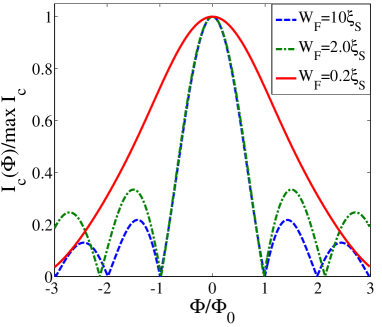
Figure 6: Magnetic interference pattern of an $S$/$F$/$S$ Josephson junction (see Fig. 5). The critical supercurrent $I_{c}(\Phi)$, is shown normalized by its maximum value, $\max(I_{c})$, and plotted against the external magnetic flux $\Phi$. Three values of the magnetic layer width $W_{F}$ are considered: $10\xi_{S}$, $2.0\xi_{S}$, and $0.2\xi_{S}$, whereas the length of $F$ is assumed fixed at a representative value of $d_{F}=2.0\xi_{S}$.

where the junction characteristics are obtained via averaged values. The critical supercurrent thus shows a monotonic decaying behavior against the external magnetic flux $\Phi$ in the narrow junction regime. This fact can be understood by noting the role of $\Gamma_{H}$ in the Usadel equations. In the narrow junction limit, the external magnetic field breaks the coherence of Cooper pairs and the Fraunhofer diffraction patterns for the critical current in the wide junction limit turns to a monotonic decay. The proximity vortices, which are closely linked to the Fraunhofer patterns, vanish in this regime due to the narrow size of junction width. This finding is also in agreement with the nonmagnetic $S$/$N$/$S$ junction counterpart Cuevas_frh1 ; Cuevas_frh2 . If we substitute the solutions from Eq. (34) into the pair potential, Eq. (IV.2.1), we find that the zeros which appeared in the wide junction limit have now vanished in the narrow junction regime. We now proceed to compliment our simplified analytical results with a more complete numerical investigation.

IV.2.3 Interference patterns, proximity vortices, and current densities: Numerical investigations

Previously we utilized various approximations to simplify situations and permit explicit analytical solutions. To investigate the validity of our analytic results, we solve numerically the Usadel equations, Eq. (19) with appropriate boundary conditions found in Eqs. (20) and (21). We now retain the $c(\varepsilon)$ terms, and include a broader range of junction widths, not only those that are very narrow or very wide, but also intermediate widths that are not amenable to an analytical treatment. We shall present results for the current density and for spatial maps of the pair potential in the junction subjected to an external magnetic field.

Figure 6 exhibits the results of our numerical studies for the critical supercurrent response to an external magnetic flux, $\Phi$, in a $S$/$F$/$S$ junction with a variety of ratios $W_{F}/d_{F}$. The junction length and exchange field intensity are fixed at particular values of $d_{F}=2.0\xi_{S}$ and $|\vec{h}|=5.0\Delta_{0}$ respectively. The interface resistance parameter is set to $\zeta=4.0$. These choices ensure the validity of the Green’s functions in the low proximity limit: $\underline{F}(x,y,z,\varepsilon)\ll 0.1\underline{F}^{no}(x,y,z,\varepsilon)$. To more clearly see the effects in the scaled plots, we normalize the critical charge supercurrent by the maximum of this quantity max($I_{c}$) for each case separately.

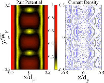
Figure 7: Spatial maps of the pair potential and current density in the presence of an external magnetic field applied normally to the plane of an $S$/$F$/$S$ Josephson junction (see Fig. 5). We assume the junction is relatively wide, $W_{F}=10\xi_{S}$, while its length is sufficiently short to allow for current transport across the $x$ axis, namely, $d_{F}=2.0\xi_{S}$. The external magnetic flux is $\Phi=3\Phi_{0}$, and the macroscopic phase difference is corresponds to $|\phi|=\pi/2$.

The figure clearly reveals a full Fraunhofer pattern for the case of a wide junction $W_{F}=10\xi_{S}$. This pattern is consistent with the analytic expression for the critical current given by Eq. (30). The critical supercurrent decays with increasing magnetic field and undergoes a series of cusps, indicating that $I_{c}$ changes sign. The observed sign-change reflects aspects of the orbital motions of the quasiparticles, while the decaying behavior is indicative of the pair breaking nature of an external magnetic field as we explained previously. A relatively narrower junction width of $W_{F}=2.0\xi_{S}$ is also investigated. As shown, the ideal Fraunhofer pattern is now modified, yet still retains its trademark signature. This diffraction pattern transitions to a uniformly decaying behavior for the sufficiently narrow junction with width $W_{F}=0.2\xi_{S}$. This narrowest junction confines the orbital motion of the quasiparticles and thus the pair-breaking by the external field plays a dominant role in the critical supercurrent response.

In Fig. 7 we plot the 2D spatial dependence of the pair potential and charge current density for a wide junction, where the larger width can more effectively demonstrate the orbital paths as they relate to the pair correlations and supercurrent response. To be consistent with Fig. 6, we set $\Phi=3\Phi_{0}$, $W_{F}=10\xi_{S}$, and $|\phi|=\pi/2$. As shown, three zeros in the pair potential appear at the middle of the junction (at $x=0$) as was found analytically in Sec. IV.2.2. The intensity of the external magnetic flux $\Phi$ determines the number of zeros and distance between neighboring zeros. The panel on the right corresponds to a spatial and vector map of the charge current density, revealing the circulating paths of the quasiparticles. If we set $|\phi|=\pi/2$ in Eq. (32), with the constraint $-1/2<y<1/2$, we find that $y=-1/12,3/12,5/12$ corresponds precisely to the zeroes of the pair potential found from the general numerical treatment, shown in Fig. 7. Likewise, $y=\pm 1/12$, $y=\pm 3/12$, and $y=\pm 5/12$ gives the zeroes of the current density. As seen, the additional zeros in the current density corresponds to locations where the trajectories of two opposing circular paths overlap, thus canceling one another. The other $y$ values giving zeroes, which correlate with the same locations as the pair potential, are at the cores of the circulating paths. Such behavior is reminiscent of Abrokosov vortices, where the supercurrent circulates around normal state cores. The zeros in the pair potential may thus be viewed as proximity vortices. Cuevas_frh2 ; Suderow ; Abrikosov1 ; Abrikosov2 ; Abrikosov3 Abrikosov vortices, which carry a single magnetic quantum flux $\Phi_{0}$, are however intrinsic to type II superconductors.Abrikosov1 ; Abrikosov2 ; Abrikosov3 ; Suderow One of the criteria for categorizing the superconducting state of a material is the nature of these intrinsic vortices.Tinkham Nonetheless, such proximity vortices are generally geometry-dependent and rely on the mutual interaction between a magnetic field with the superconductor, in contrast to intrinsic Abrikosov vortices. Cuevas_frh2

IV.3 Spin-parametrization

The Usadel equations in this section have dealt solely with the even-frequency superconducting correlations with spin-zero projection along the spin-quantization axis. This is due to the fact that we have only considered ferromagnetic strips with a uniform magnetization texture. For inhomogeneous magnetization textures, the complex partial differential equations become coupled and increase in number to eight in the low proximity limit. This number is doubled if the full proximity limit alidoust1 is considered. Fortunately, it has been well established that the low proximity limit is sufficient to capture the essential physical properties of proximity systems such as the ones proposed in this paper. To investigate the behavior of even- and odd-frequency correlations, we employ a spin-parametrization techniqueLofwander2 ; Champel1 ; Champel2 that has been frequently used to study the characteristics of magnetic systems. Lofwander2 ; Champel1 ; Champel2 ; Hikino ; alidoust_missner ; buzdin1 ; Houzet1 ; Oboznov ; bergeret1 ; bergeret2

If we now substitute this decomposition of the anomalous Green’s function into the Usadel equation, Eq. (II.1), and consider a two-dimensional system, we end up with the following coupled set of differential equations in the presence of an external flux $\Phi$:

$$D\bigg{\{}\mp\partial_{x}^{2}\mathbb{T}_{x}(-\varepsilon)\mp\Big{(}\frac{d_{F}}{W_{F}}\Big{)}^{2}\partial_{y}^{2}\mathbb{T}_{x}(-\varepsilon)+i\partial_{x}^{2}\mathbb{T}_{y}(-\varepsilon)+i\Big{(}\frac{d_{F}}{W_{F}}\Big{)}^{2}\partial_{y}^{2}\mathbb{T}_{y}(-\varepsilon)+4i\Phi y(\mp\partial_{x}\mathbb{T}_{x}(-\varepsilon)+i\partial_{x}\mathbb{T}_{y}(-\varepsilon))\bigg{.}$$

$$\bigg{.}-4\Phi^{2}y^{2}(\mp\mathbb{T}_{x}(-\varepsilon)+i\mathbb{T}_{y}(-\varepsilon))\bigg{\}}+id_{F}^{2}\Big{\{}\mathbb{T}_{y}-2\varepsilon(\mp\mathbb{T}_{x}(-\varepsilon)+i\mathbb{T}_{y}(-\varepsilon))\mp 2\mathbb{S}(-\varepsilon)(h^{x}\mp ih^{y})\Big{\}}=0,$$ (36a)

$$D\bigg{\{}\mp\partial_{x}^{2}\mathbb{S}(-\varepsilon)\mp\Big{(}\frac{d_{F}}{W_{F}}\Big{)}^{2}\partial_{y}^{2}\mathbb{S}(-\varepsilon)+\partial_{x}^{2}\mathbb{T}_{z}(-\varepsilon)+\Big{(}\frac{d_{F}}{W_{F}}\Big{)}^{2}\partial_{y}^{2}\mathbb{T}_{z}(-\varepsilon)+4i\Phi y(\mp\partial_{x}\mathbb{S}(-\varepsilon)+\partial_{x}\mathbb{T}_{z}(-\varepsilon))\bigg{.}$$

$$\bigg{.}-4\Phi^{2}y^{2}(\mp\mathbb{S}(-\varepsilon)+\mathbb{T}_{z}(-\varepsilon))\bigg{\}}+id_{F}^{2}\Big{\{}\mp 2\mathbb{T}_{x}(-\varepsilon)h^{x}\mp 2\mathbb{T}_{y}(-\varepsilon)h^{y}-2(\mp\mathbb{S}(-\varepsilon)+\mathbb{T}_{z}(-\varepsilon))(\varepsilon\pm h^{z})\Big{\}}=0,$$ (36b)

$$D\bigg{\{}\mp\partial_{x}^{2}\mathbb{T}_{x}^{\ast}(\varepsilon)\mp\Big{(}\frac{d_{F}}{W_{F}}\Big{)}^{2}\partial_{y}^{2}\mathbb{T}_{x}^{\ast}(\varepsilon)-i\partial_{x}^{2}\mathbb{T}_{y}^{\ast}(\varepsilon)-i\Big{(}\frac{d_{F}}{W_{F}}\Big{)}^{2}\partial_{y}^{2}\mathbb{T}_{y}^{\ast}(\varepsilon)-4i\Phi y(\mp\partial_{x}\mathbb{T}_{x}^{\ast}(\varepsilon)-i\partial_{x}\mathbb{T}_{y}^{\ast}(\varepsilon))\bigg{.}$$

$$\bigg{.}-4\Phi^{2}y^{2}(\mp\mathbb{T}_{x}^{\ast}(\varepsilon)-i\mathbb{T}_{y}^{\ast}(\varepsilon))\bigg{\}}+id_{F}^{2}\Big{\{}\pm 2(h^{x}\pm ih^{y})\mathbb{S}^{\ast}(\varepsilon)-2\varepsilon(\mp\mathbb{T}_{x}^{\ast}(\varepsilon)-i\mathbb{T}_{y}^{\ast}(\varepsilon))\Big{\}}=0,$$ (36c)

$$D\bigg{\{}\mp\partial_{x}^{2}\mathbb{S}^{\ast}(\varepsilon)\mp\Big{(}\frac{d_{F}}{W_{F}}\Big{)}^{2}\partial_{y}^{2}\mathbb{S}^{\ast}(\varepsilon)+\partial_{x}^{2}\mathbb{T}_{z}^{\ast}(\varepsilon)+\Big{(}\frac{d_{F}}{W_{F}}\Big{)}^{2}\partial_{y}^{2}\mathbb{T}_{z}^{\ast}(\varepsilon)-4i\Phi y(\mp\partial_{x}\mathbb{S}^{\ast}(\varepsilon)+\partial_{x}\mathbb{T}_{z}^{\ast}(\varepsilon))\bigg{.}$$

$$\bigg{.}-4\Phi^{2}y^{2}(\mp\mathbb{S}^{\ast}(\varepsilon)+\mathbb{T}_{z}^{\ast}(\varepsilon))\bigg{\}}+id_{F}^{2}\Big{\{}2(-\varepsilon\pm h^{z})(\mp\mathbb{S}^{\ast}(\varepsilon)+\mathbb{T}_{z}^{\ast}(\varepsilon))\pm 2h^{x}\mathbb{T}_{x}^{\ast}(\varepsilon)\pm 2h^{y}\mathbb{T}_{y}^{\ast}(\varepsilon)\Big{\}}=0.$$ (36d)

The spin parameterized boundary conditions at the left $S$/$F$ interface, Eq. (II.1), now reads:

$$\Big{\{}\zeta(\partial_{x}+2i\Phi y)-c^{\ast}(\varepsilon)\Big{\}}\Big{(}\mp\mathbb{T}_{x}(-\varepsilon)+i\mathbb{T}_{y}(-\varepsilon)\Big{)}=0,$$ (37a)

$$\Big{\{}\zeta(\partial_{x}+2i\Phi y)-c^{\ast}(\varepsilon)\pm i\frac{G_{S}}{G_{T}}\Big{\}}\Big{(}\mp\mathbb{S}(-\varepsilon)+\mathbb{T}_{z}(-\varepsilon)\Big{)}\pm s^{\ast}(\varepsilon)e^{i\theta_{l}}=0,$$ (37b)

$$\Big{\{}\zeta(\partial_{x}-2i\Phi y)-c^{\ast}(\varepsilon)\Big{\}}\Big{(}\mp\mathbb{T}_{x}^{\ast}(\varepsilon)-i\mathbb{T}_{y}^{\ast}(\varepsilon)\Big{)}=0,$$ (37c)

$$\Big{\{}\zeta(\partial_{x}-2i\Phi y)-c^{\ast}(\varepsilon)\mp i\frac{G_{S}}{G_{T}}\Big{\}}\Big{(}\mp\mathbb{S}^{\ast}(\varepsilon)+\mathbb{T}_{z}^{\ast}(\varepsilon)\Big{)}\mp s^{\ast}(\varepsilon)e^{-i\theta_{l}}=0,$$ (37d)

and for the right $S$/$F$ interface, we have:

$$\Big{\{}\zeta(\partial_{x}+2i\Phi y)+c^{\ast}(\varepsilon)\Big{\}}\Big{(}\mp\mathbb{T}_{x}(-\varepsilon)+i\mathbb{T}_{y}(-\varepsilon)\Big{)}=0,$$ (38a)

$$\Big{\{}\zeta(\partial_{x}+2i\Phi y)+c^{\ast}(\varepsilon)\mp i\frac{G_{S}}{G_{T}}\Big{\}}\Big{(}\mp\mathbb{S}(-\varepsilon)+\mathbb{T}_{z}(-\varepsilon)\Big{)}\mp s^{\ast}(\varepsilon)e^{i\theta_{r}}=0,$$ (38b)

$$\Big{\{}\zeta(\partial_{x}-2i\Phi y)+c^{\ast}(\varepsilon)\Big{\}}\Big{(}\mp\mathbb{T}_{x}^{\ast}(\varepsilon)-i\mathbb{T}_{y}^{\ast}(\varepsilon)\Big{)}=0,$$ (38c)

$$\Big{\{}\zeta(\partial_{x}-2i\Phi y)+c^{\ast}(\varepsilon)\pm i\frac{G_{S}}{G_{T}}\Big{\}}\Big{(}\mp\mathbb{S}^{\ast}(\varepsilon)+\mathbb{T}_{z}^{\ast}(\varepsilon)\Big{)}\pm s^{\ast}(\varepsilon)e^{-i\theta_{r}}=0.$$ (38d)

Using Eq. (8), the spin-parameterized current density through the junction (along the $x$ direction) in the presence of an external magnetic field is:

$$J_{x}(x,y)= J_{0}\int_{-\infty}^{\infty}d\varepsilon\bigg{\{}\bigg{.}\mathbb{S}(\varepsilon)\partial_{x}\mathbb{S}^{\ast}(-\varepsilon)-\mathbb{S}(-\varepsilon)\partial_{x}\mathbb{S}^{\ast}(\varepsilon)+\mathbb{S}(\varepsilon)^{\ast}\partial_{x}\mathbb{S}(-\varepsilon)-\mathbb{S}(-\varepsilon)^{\ast}\partial_{x}\mathbb{S}(\varepsilon)-\partial_{x}\mathbb{T}_{x}(-\varepsilon)\mathbb{T}_{x}^{\ast}(\varepsilon)+\partial_{x}\mathbb{T}_{x}(\varepsilon)\mathbb{T}_{x}^{\ast}(-\varepsilon)$$ (39)

$$\left.-\right.\left.\partial_{x}\mathbb{T}_{x}^{\ast}(-\varepsilon)\mathbb{T}_{x}(\varepsilon)+\partial_{x}\mathbb{T}_{x}^{\ast}(\varepsilon)\mathbb{T}_{x}(-\varepsilon)-\partial_{x}\mathbb{T}_{y}(-\varepsilon)\mathbb{T}_{y}^{\ast}(\varepsilon)+\partial_{x}\mathbb{T}_{y}(\varepsilon)\mathbb{T}_{y}^{\ast}(-\varepsilon)-\partial_{x}\mathbb{T}_{y}^{\ast}(-\varepsilon)\mathbb{T}_{y}(\varepsilon)+\partial_{x}\mathbb{T}_{y}^{\ast}(\varepsilon)\mathbb{T}_{y}(-\varepsilon)\right.$$

$$\left.-\right.\left.\partial_{x}\mathbb{T}_{z}(-\varepsilon)\mathbb{T}_{z}^{\ast}(\varepsilon)+\partial_{x}\mathbb{T}_{z}(\varepsilon)\mathbb{T}_{z}^{\ast}(-\varepsilon)-\partial_{x}\mathbb{T}_{z}^{\ast}(-\varepsilon)\mathbb{T}_{z}(\varepsilon)+\partial_{x}\mathbb{T}_{z}^{\ast}(\varepsilon)\mathbb{T}_{z}(-\varepsilon)-4i\Phi y\Big{[}\mathbb{S}(\varepsilon)\mathbb{S}^{\ast}(-\varepsilon)-\mathbb{S}(-\varepsilon)\mathbb{S}^{\ast}(\varepsilon)\right.$$

$$+\mathbb{T}_{x}(-\varepsilon)\mathbb{T}_{x}^{\ast}(\varepsilon)-\mathbb{T}_{x}(\varepsilon)\mathbb{T}_{x}^{\ast}(-\varepsilon)+\Big{.}\bigg{.}\Big{.}\mathbb{T}_{y}(-\varepsilon)\mathbb{T}_{y}^{\ast}(\varepsilon)-\mathbb{T}_{y}(\varepsilon)\mathbb{T}_{y}^{\ast}(-\varepsilon)+\mathbb{T}_{z}(-\varepsilon)\mathbb{T}_{z}^{\ast}(\varepsilon)-\mathbb{T}_{z}(\varepsilon)\mathbb{T}_{z}^{\ast}(-\varepsilon)\Big{]}\bigg{\}}\tanh(\varepsilon\beta).$$

The $y$ component of the supercurrent density, $J_{y}(x,y)$, takes the same form as $J_{x}(x,y)$, with the partial-$x$ derivatives replaced by derivatives with respect to $y$, and also the inclusion of the appropriate component of the vector potential.

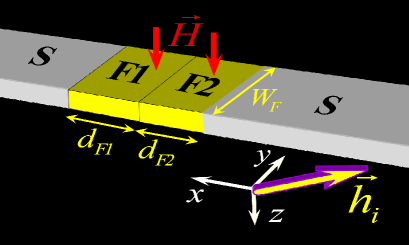
Figure 8: Proposed setup of an $S$/$F$/$F$/$S$ Josephson junction where the double layer $F$ region has its interfaces parallel with the $S$/$F$ interfaces. The ferromagnetic layers and $s$-wave superconducting terminals are labeled by $F_{1}$, $F_{2}$, and $S$, respectively. Our theoretical technique allows consideration of exchange fields with arbitrary orientations. We thus denote the magnetization of each $F$ layer by $\vec{h}_{i}=(h_{i}^{x},h_{i}^{y},h_{i}^{z})$, for $i=1,2$. The width of the rectangular $F$ strips are equal and denoted by $W_{F}$, while the length of each magnetic layer can differ and are denoted $d_{F1}$, and $d_{F2}$. The junction is located in the $xy$ plane and all interfaces are along the $y$ axis. An external magnetic field $\vec{H}$ points along the $z$ axis, normal to the junction plane.

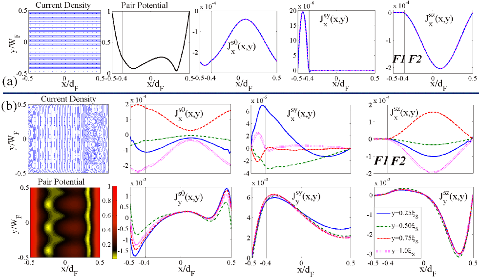
Figure 9: Spatial maps of the total critical current density, pair potential, and supercurrent components in an $S$/$F$/$F$/$S$ Josephson junction for the configuration depicted in Fig. 8. The supercurrent is decomposed into its even ($J^{s0}_{x,y}(x,y)$) and odd-frequency ($J^{sy}_{x,y}(x,y),J^{sz}_{x,y}(x,y)$) components. The two ferromagnetic layers have unequal lengths: $d_{F1}=0.2\xi_{S}$, and $d_{F2}=1.8\xi_{S}$, while their widths are equal: $W_{F1}=W_{F2}=2.0\xi_{S}$. The vertical lines identify the two ferromagnetic regions labeled $F_{1}$ and $F_{2}$. In part (a), there is no applied magnetic field, while in part (b) the external magnetic field corresponds to a flux of $\Phi=3\Phi_{0}$. The critical current components in both cases, (a) and (b), are plotted as a function of $x$-position at four different locations along the junction width: $y=0.25\xi_{S},0.50\xi_{S},0.75\xi_{S},1.0\xi_{S}$.

Incorporating the spin-parametrization, Eq. (11), into the expression for the pair potential, Eq. (10), we end up with the following compact equation:

$$\tilde{U}_{\text{pair}}=\int_{-\infty}^{+\infty}d\varepsilon\Big{\{}\mathbb{S}(\varepsilon)-\mathbb{S}(-\varepsilon)\Big{\}}\tanh(\varepsilon\beta).$$ (40)

Thus, the pair potential involves only even-frequency components of the parameterized Green’s function, consistent with the presence of a singlet order parameter in the left and right superconducting banks. In the next subsections, we solve the above equations for two different magnetization configurations, with and without an external magnetic field. The spin-parametrization outlined here will then delineate the various contributions the singlet and triplet correlations make to the supercurrent.

IV.4 $S$/$F$/$F$/$S$ heterostructures: parallel $F$/$F$ and $S$/$F$ interfaces

Employing the spin-parametrization with the Usadel equations together with the boundary conditions given in the previous section, we numerically study the proximity induced triplet correlations in a two-dimensional magnetic $S$/$F$/$F$/$S$ Josephson junction. Here the $F$/$F$ interface is parallel with the outer $S$ interfaces. The configuration is depicted in Fig. 8. The system is subject to an external magnetic field $\vec{H}$ and we study the behavior of the corresponding spin-triplet correlations. We also compare these results with the case of no external magnetic field. As exhibited in Fig. 8, the external magnetic flux is directed along the $z$ direction, normal to the junction face which resides in the $xy$ plane so that the $S$/$F$ and $F$/$F$ interfaces are parallel to the $y$ axis. We consider a rather general situation for the lengths and magnetization directions of the $F$ strips. The lengths of the $F$ strips can be unequal and are labeled by $d_{F1}$ and $d_{F2}$ ($d_{F1}\neq d_{F2}$). The strength of the exchange fields in both $F$ regions are equal $|\vec{h_{1}}|=|\vec{h_{2}}|=5.0\Delta_{0}$, while their orientations take arbitrary directions $\vec{h}_{1,2}=(h^{x}_{1,2},h^{y}_{1,2},h^{z}_{1,2})$. Also, the junction width is equal to the width of the $F$ stripes, i.e., $W_{F1}=W_{F2}\equiv W_{F}$.

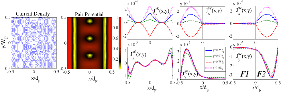
Figure 10: Spatial maps of the critical current density and pair potential as well as the critical charge current components for a junction configuration shown in Fig. 8. The same investigation as Fig. 9(b) is done here except we set $d_{F1}=d_{F2}=1.0\xi_{S}$. The junction width and external magnetic flux are $W_{F}=2.0\xi_{S}$ and $\Phi=3\Phi_{0}$, respectively. The vertical lines in the panels for the critical charge current components show the spatial separation of the two magnetic regions labeled $F_{1}$ and $F_{2}$. The quantities $J_{x}^{\beta}(x,y)$ show the current components for flow along the $x$ direction whereas $J_{y}^{\beta}(x,y)$ represents the components for flow along the $y$ direction. Here $\beta$ denotes a specific component of the decomposed charge supercurrent namely, $s0$, $sx$, $sy$, and $sz$.

The charge supercurrent given by Eq. (39) is comprised of even-frequency singlet terms, $\mathbb{S}$, and the triplet odd-frequency components, $\vec{\mathbb{T}}$. To study exactly the behavior of each component of the Josephson charge current, we introduce the following decomposition scheme which is based on the discussions and notations in the previous sections:

$$\text{terms involving $\mathbb{S}$}\;\;\;\;\;\;\Rightarrow\;\;\;\;J^{s0}_{x,y},$$ (41a)

$$\text{terms involving $\mathbb{T}_{x}$}\;\;\;\;\Rightarrow\;\;\;\;J^{sx}_{x,y},$$ (41b)

$$\text{terms involving $\mathbb{T}_{y}$}\;\;\;\;\Rightarrow\;\;\;\;J^{sy}_{x,y},$$ (41c)

$$\text{terms involving $\mathbb{T}_{z}$}\;\;\;\;\Rightarrow\;\;\;\;J^{sz}_{x,y}.$$ (41d)

In order to explicitly study the influence of each component of the decomposed charge supercurrent, we fix the magnetization of the $F_{1}$ wire to be in the $y$-direction: $\vec{h}_{1}=(0,h^{y},0)$. Similarly, the magnetization of $F_{2}$ is orthogonal to that of $F_{1}$, and oriented in the $z$ direction: $\vec{h}_{2}=(0,0,h^{z})$. This orthogonal magnetization configuration is an inhomogeneous magnetic state that results in effective generation of equal-spin triplet correlationsbergeret1 .

We show the spatial behavior of the total charge supercurrent density, pair potential, and the supercurrent components for a phase difference of $|\phi|=\pi/2$ in Fig. 9 for the $S$/$F$/$F$/$S$ junction depicted in Fig. 8. The geometric dimensions correspond to $d_{F1}=0.2\xi_{S}$, $d_{F2}=1.8\xi_{S}$, and the junction width $W_{F}$ is set equal to $2.0\xi_{S}$. The selected values of $d_{F}=d_{F1}+d_{F2}$ and $W_{F}$ are useful towards understanding and analyzing the spin-triplet correlations in the different $S$/$F$/$F$/$S$ Josephson junctions considered here. For the panels found in (a), the external magnetic flux is absent, while for those in (b), a magnetic flux $\Phi=3\Phi_{0}$ is applied to the system. In panels (a), the charge current density is conserved as exhibited by its spatial uniformity throughout the ferromagnetic wire regions. There is also no $y$ variations due the layered system exhibiting translational invariance in that direction. Without an external magnetic field, the charge supercurrent (and pair potential) thus have no components along the $y$ direction. The pair potential is shown to be an asymmetric function of position along the junction, which is simply due to the unequal length of each $F$ wire and their differing magnetizations. The charge supercurrent density components, $J_{x}^{s0}$, $J_{x}^{sy}$, and $J_{x}^{sz}$, are also shown. These quantities can only vary spatially in the $x$-direction too since in the absence of an external field, the total supercurrent is generated from the phase difference $\phi$ between the $S$ terminals, which vary only along the junction length ($x$ direction). The odd-frequency triplet components of the supercurrent are localized in the $F_{1}$ or $F_{2}$ regions depending on the specific magnetization orientation in each region (see also the discussion in Sec. III). It is evident that $J_{x}^{sy}$ disappears in the right $F$ while $J_{x}^{sz}$ is zero inside $F_{1}$ segment where $\vec{h}_{1}=(0,h^{y}_{1},0),\vec{h}_{2}=(0,0,h^{z}_{2})$, respectively ($\vec{h}_{1}\rightarrow J^{sy}$, $\vec{h}_{2}\rightarrow J^{sz}$). Thus $J^{sy}$ is generated in $F_{1}$ and at the $F$/$F$ interface is converted into $J^{sz}$ in $F_{2}$, or vice versa. The two components are generated in one $F$ and do not penetrate into the other $F$ with orthogonal magnetization. Turning now to Fig. 9(b), a finite magnetic flux of $\Phi=3\Phi_{0}$ results now in a nonuniform supercurrent response that varies in both the $x$ and $y$ directions. Examining now the singlet correlations, the pair potential asymmetry is again present due to the spatially asymmetric magnetization regions, while the external magnetic field induces vortices with normal state cores along the junction width. The singlet and triplet components of the supercurrent are plotted as well. The external magnetic field makes the problem effectively two dimensional, as it induces nonzero current densities in the $y$ direction. The amplitude of the equal-spin triplet component in the $x$-direction, $J^{sy}_{x}(x,y)$, is somewhat smaller than the other components due in part to the small $F_{1}$ width, $d_{F1}=0.2\xi_{S}$. However, comparing $J^{sy}_{x}(x,y)$ in panels (a) and (b), we see that the presence of a magnetic field can result in this triplet component now existing in $F_{2}$, and it can also be more prominent in $F_{1}$.

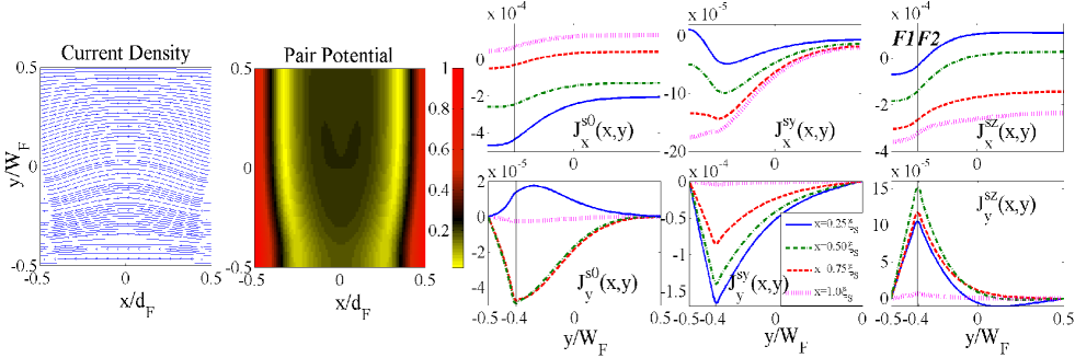
Figure 11: Spatial maps of the maximum total charge current, pair potential, and the even- ($J^{s0}_{x,y}(x,y)$) and odd-frequency ($J^{sx}_{x,y}(x,y),J^{sy}_{x,y}(x,y),J^{sz}_{x,y}(x,y)$) components of the charge current. The configuration of the $S$/$F$/$F$/$S$ Josephson junction considered here is shown in Fig. 12. The $F$/$F$ interface is now perpendicular to the $S$/$F$ interfaces. The external magnetic flux is zero, $\Phi=0$, and the junction length $d_{F}$ is equal to $2.0\xi_{S}$. The width of each ferromagnetic strip are unequal, i.e., $W_{F1}=0.2\xi_{S}$ and $W_{F2}=1.8\xi_{S}$. The current components are plotted against the lateral $y$ coordinate, i.e., along the junction width. Four various locations along the junction length are considered: $x=0.25\xi_{S}$, $0.50\xi_{S}$, $0.75\xi_{S}$, and $1.0\xi_{S}$. Vertical lines in the panels for the current components separate the two ferromagnetic regions along the $y$ direction (see Fig. 12).

Turning now to the $y$ components of the currents, we see that the magnitudes have increased in most instances by almost an order of magnitude or more. Although $J^{s0}_{y}(x,y),J^{sy}_{y}(x,y)$, and $J^{sz}_{y}(x,y)$ vary little at the different $y$ locations, the overall spatial behavior is different for the odd and even frequency triplet components: The equal spin $J^{sy}_{y}(x,y)$ penetrates considerably more into the ferromagnetic regions compared with its $x$-component counterpart and compared with the spin-0 triplet $J^{sz}_{y}(x,y)$. These results are consistent with the generation of a Meissner supercurrent in $S$/$F$/$F$/$N$ structures.alidoust_missner .

To study the effects of varying the system geometry and its corresponding effects on the triplet supercurrents, we consider more symmetric $F$ regions with equal lengths $d_{F1}=d_{F2}=1.0\xi_{S}$. All other parameters are identical to the previous $S$/$F$/$F$/$S$ junction in Fig. 9(b). The first two panels on the left of Fig. 10 illustrate 2D spatial maps of the total supercurrent density and pair potential. The remaining panels contain the spatial behavior of the singlet and triplet contributions to the total current. The effect of equal layer widths is reflected in the regular array of vortex patterns and circulating currents in the junction. The pair potential at $x=0$ exhibits three zeros when $\Phi=3\Phi_{0}$. This is in accordance with the analytic expression in Eq. (32) and Eq. (40) which demonstrates the actual behavior of singlet correlations, constituting the spatial profile of proximity pair potential. To reveal the even and odd frequency contributions to the contour plots, we examine in the remaining panels the supercurrent components as a function of $x$. The vertical lines separate the two ferromagnetic regions labeled by $F_{1}$ and $F_{2}$, as shown in the schematic of Fig. 8. We see that the formerly long-ranged $J_{y}^{sy}(x,y)$ and $J_{y}^{sz}(x,y)$, in Fig. 9 now vanish here when $d_{F1}=d_{F2}=1.0\xi_{S}$.

Figure 12: Schematic of the $S$/$F$/$F$/$S$ Josephson junction where the interface of the double ferromagnet region is oriented perpendicular to the $S$/$F$ interfaces. The junction is located in the $xy$ plane and the $S$/$F$ interfaces are along the $y$ axis while the $F$/$F$ interface is along the $x$ axis. The width of the rectangular $F$ strips $W_{F1}$, and $W_{F2}$ are generally unequal, i.e., $W_{F1}\neq W_{F2}$. The lengths of the $F$ strips, $d_{F}$, however, are the same and correspond to the junction length. An external magnetic field $\vec{H}$ is applied normal to the junction plane along the $z$ axis.

This demonstrates the crucial role that geometry can play in these type of junctions, in particular the existence of odd-frequency correlations tend to favor configurations where the length of the ferromagnetic layers are unequal, for instance, $d_{F2}\gg d_{F1}$ can further enhance the effect. This finding is also consistent with the results of a $S$/$F$/$F$/$N$ configuration subjected to an external magnetic field,alidoust_missner where the $J_{x}^{sy}$ component of the Meissner current is optimally anomalous if $d_{F2}\gg d_{F1}$. The behavior of the singlet and triplet correlations discussed here are typically highly dependent on the magnetization of the double $F$ layer, as well as the presence of an external magnetic field. In the next section, we therefore proceed to investigate another type of $S$/$F$/$F$/$S$ Josephson junction with a different double $F$ layer arrangement.

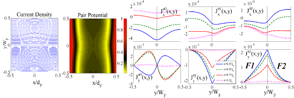
Figure 13: Spatial maps depicting a vector plot of the total charge current density and density plot of the pair potential for the system shown in Fig. 12. The remaining line plots correspond to the charge supercurrent components: the singlet, $J^{s0}_{x,y}(x,y)$, and triplets, $J^{sy}_{x,y}(x,y),J^{sz}_{x,y}(x,y)$. Here the system parameters are identical to those used previously in Fig. 11, except the width of the ferromagnetic strips here are equal: $W_{F1}=W_{F2}=1.0\xi_{S}$. The junction length $d_{F}$ is equal to $2.0\xi_{S}$ and there is no external magnetic flux, $\Phi=0$. The vertical lines indicate the locations of the $F$/$F$ interfaces in between the two ferromagnetic regions $F_{1}$ and $F_{2}$.

IV.5 $S$/$F$/$F$/$S$ heterostructures: $F$/$F$ interface perpendicular to $S$/$F$ interfaces

Here we consider a type of $S$/$F$/$F$/$S$ Josephson junction where the previous ferromagnet double layer system is rotated by $\pi/2$, so that the $F$/$F$ interface is normal to the outer $S$/$F$ interfaces. This layout is shown in Fig. 12. As before, we take the length of the ferromagnetic strips to be equal, $d_{F1}=d_{F2}\equiv d_{F}$. We first consider ferromagnets where the width of the $F_{1}$ and $F_{2}$ regions are unequal: $W_{F1}\neq W_{F2}$. When an applied magnetic field, $\vec{H}$, is present, it is directed along the $z$-axis, normal to the plane of the system. To be consistent with the previous subsection, we study two regimes of ferromagnetic widths namely, $W_{F1}\ll W_{F2}$ and $W_{F1}=W_{F2}$, and investigate how the results vary for a finite external magnetic flux $\Phi$.

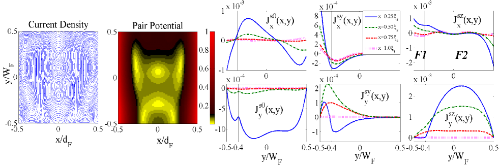
Figure 14: Spatial maps of total critical charge current density and pair potential and the decomposed components of charge supercurrent $J^{s0}_{x,y}(x,y),J^{sx}_{x,y}(x,y),J^{sy}_{x,y}(x,y),J^{sz}_{x,y}(x,y)$. The same parameter set as Fig. 11 are used except we now assume the system is subject to an external magnetic flux $\Phi=3\Phi_{0}$. The vertical lines in the current components’ panels separate the two ferromagnetic segments, labeled by $F_{1}$, and $F_{2}$, with orthogonal magnetization orientations. The current components are plotted as a function of positions along the junction width i.e. $y$ direction at four locations along the junction length i.e. $x=0.25\xi_{S}$, $0.50\xi_{S}$, $0.75\xi_{S}$, and $1.0\xi_{S}$.

In Fig. 11, we show the results for $W_{F1}=0.2\xi_{S}$, and $W_{F2}=1.8\xi_{S}$, in the absence of an applied magnetic field ($\Phi=0$). First, the spatial map of the total maximum charge supercurrent shows that the current near the $F$/$F$ junction has a non-zero $y$-component. This is in contrast to the uniform supercurrent shown in Fig. 9(a) for a “parallel” $F$/$F$ segment. The induced $y$ component is present over the entire junction width as exhibited by the distorted quasiparticle paths. The pair potential shows a symmetric behavior along the junction length (the $x$ direction). However, similar to the previous case, the pair potential is an asymmetric function of $y$ coordinate. This again arises from the unequal ferromagnetic wire widths ($W_{F1}\neq W_{F2}$) and their different magnetization orientations. The spatial behavior of the triplet and singlet contributions to the supercurrent is also shown as a function of position along the junction width (the $y$ direction) at four $x$ locations: $x=0.25\xi_{S},0.5\xi_{S},0.75\xi_{S},1.0\xi_{S}$. The amplitude of $J_{y}^{s0}$ is around $\approx 1/10$ of $J_{y}^{sy}$ and $J_{y}^{sz}$ but comparable with $|J_{y}^{sy}+J_{y}^{sz}|$. These components of $J_{y}$, and hence $J_{y}$ itself, vanish at $y=\pm 0.5$, corresponding to the vacuum boundary, and consistent with the boundary conditions given by Eq. (II.1). The vector plot of the charge supercurrent in Fig. 11 reveals no current flow along $y$ in the middle of the junction, $x=0$, throughout the junction width. The $x$ component, $J_{x}^{s0}$, is most negative at $x=0$ along the $y$ axis while $J_{x}^{sy}$ and $J_{x}^{sz}$ are maximal. Therefore, the singlet-triplet conversion with $W_{F2}\gg W_{F1}$ is maximal at $x=0$. Another important aspect of this $S$/$F$/$F$/$S$ junction is seen in the behavior of $J_{x}^{sy}$ and $J_{x}^{sz}$ as a function of $y$: the two components are generated in one $F$ region and penetrate deeply into the adjacent $F$ segment. By comparing these plots with those of a $S$/$F$/$F$/$S$ configuration where $F$/$F$ interface is parallel with the $S$/$F$ interface subjected to an external magnetic field, presented in Fig. 9(b), one concludes that the spin-1 triplet components of charge supercurrent can penetrate the ferromagnetic regions when they flow parallel to the junction interfaces.

In Fig. 13, we investigate the geometrical effects on the superconducting properties for a system with $F_{1}$ and $F_{2}$ of equal width. We have $W_{F1}=W_{F2}=1.0\xi_{S}$, and all previous parameters remain intact. The current density map shows that the the induced $y$-component is equally distributed with respect to $y=0$, the location of the $F$/$F$ interface. The pair potential is a symmetric function of both the $x$ and $y$ coordinates about the origin, reflecting the symmetric geometric configuration. The panels representing the current components reveal that the $y$-component to the current density originates mainly from the singlet term, $J_{y}^{s0}$, since it is evident that the odd-frequency components $J_{y}^{sy}$ and $J_{y}^{sz}$ are of opposite sign so that $J_{y}^{sy}+J_{y}^{sz}\approx 0$. Note that $J_{y}^{s0}$ is an odd function of $y$ for each fixed $x$-location. This reflects the fact that the junction is symmetric along the $y$ direction (see Fig. 11). From the current density spatial map the same functionality appears for the $x$ coordinate. The integration $\int_{-0.5}^{0.5}dxJ_{y}^{s0}$ gives the total charge supercurrent flowing in the $y$ direction which is therefore zero due since $J_{y}^{s0}$ is antisymmetric in $y$. For the previous case shown in Fig. 11, both triplet components $J_{y}^{sy}$ and $J_{y}^{sz}$ contributed to the induced $y$ component in the total current density. Considering now the flow of current along the $x$ direction, the top panels display the behavior of the odd-frequency triplet components with spin-1 and spin-0 projections on the $z$ quantization axes ($J_{x}^{sy}$ and $J_{x}^{sz}$, respectively). Interestingly, the generation of each of the two triplet components tends to mirror each others behavior. Since the ferromagnetic regions are symmetric, the singlet-triplet conversion of charge supercurrent components at the middle of junction ($x=0$) across the junction is not as extensive compared to the previous case where $W_{F2}\gg W_{F1}$. It is clear that the total current passing through the junction must be conserved along the junction length ($I_{tot}(x)=const.$). However, the singlet-triplet conversion in the charge supercurrent density is maximal at $x=0$ and increases as the condition $W_{F2}\gg W_{F1}$ is fulfilled.

In the previous two figures, the source of the driving current was the macroscopic phase differences between the $S$ terminals in the Josephson structures. We now introduce an additional source and associated triplet correlations by applying an external magnetic field (with corresponding flux $\Phi=3\Phi_{0}$), normal to the junction plane along the $z$-axis (see schematic, Fig. 12). Therefore, Fig. 14 exhibits our results for a junction with the same parameters used in Fig. 11 but now, $\Phi=3\Phi_{0}$. The magnetic field causes the quasiparticles to undergo circular motion as shown in the vector plot for the supercurrent density. The pair potential also vanishes at particular locations, which now form a nontrivial pattern. The charge supercurrent components are clearly modified by the external magnetic field compared to $\Phi=0$ (Fig. 11). We have found that the behavior of the supercurrent components along $y$ are similar to the corresponding components along $x$ when the $F$/$F$ junction is parallel with the $S$/$F$ interfaces (Fig. 9(b)). In both cases, the supercurrent flows normal to the $F$/$F$ junction. Likewise, the $J_{x}$ component as a function of $y$ in Fig. 11 is similar to the $J_{y}$ component vs. $x$ as seen in Fig. 9(b). Recall that in Fig. 14, we have $\Phi=3\Phi_{0}$, while in Fig. 9(b) $\Phi=0$. Here we find also that the triplet components of the charge supercurrent generated in one $F$ strip, flowing parallel with the $F$/$F$ interface deeply penetrate the adjacent $F$ compared to when the current flows normal to the $F$/$F$ interface. It is also evident that the total net supercurrent in the $y$ direction is zero, i.e., $\int_{-0.5}^{+0.5}dx(J_{y}^{s0}+J_{y}^{sy}+J_{y}^{sz})=0$.

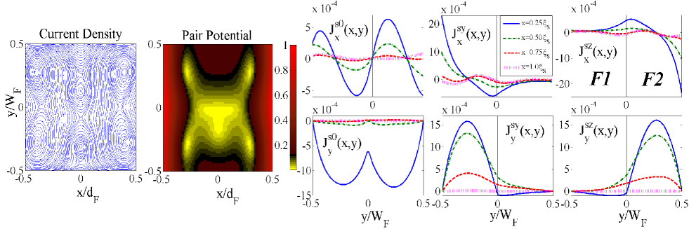
Figure 15: Spatial maps of the total charge supercurrent and pair potential in addition to the current components $J^{s0}_{x,y}(x,y),J^{sx}_{x,y}(x,y),J^{sy}_{x,y}(x,y),J^{sz}_{x,y}(x,y)$, at maximum charge current flowing across the junction. The same investigations as Fig. 13 are presented here. The junction length is fixed at $d_{F}=2.0\xi_{S}$ while the width of each ferromagnetic strip, labeled by $F_{1}$ and $F_{2}$, are $W_{F1}=W_{F2}=1.0\xi_{S}$. Unlike Fig. 13, the external magnetic flux is $\Phi=3\Phi_{0}$. The two ferromagnetic regions with orthogonal magnetization orientations are separated by vertical lines and labeled $F_{1}$ and $F_{2}$.

Upon changing the width of the $F$ layers to $W_{F1}=W_{F2}=1.0\xi_{S}$, Fig. 15 shows that the circular paths observed in the current density and zeroes in the spatial map of the pair potential have reverted back to a more symmetric configuration compared to Fig. 14. Here the magnetization orientations in the $F$ regions are orthogonal: $\vec{h}_{1}=(0,h^{y},0)$, and $\vec{h}_{2}=(0,0,h^{z})$. The panels containing the current components $J_{x}^{sy}$ and $J_{x}^{sz}$ as a function of $y$ are now much more localized in the $F$ regions, in contrast to the previous case where $W_{F2}\gg W_{F1}$ (Fig. 11). Considering the current density along the $y$ direction, the triplet components are also localized in the $F$ regions. Similarities are observed when comparing their $y$ dependence with the $x$ dependence of the triplets $J_{x}^{sy}$ and $J_{x}^{sz}$ in Fig. 10. This comprehensive investigation into the different $S$/$F$/$F$/$S$ structures has shown that an applied magnetic field can result in the appearance of odd-frequency triplet components to the charge transport when the supercurrent is parallel to the $F$/$F$ interface. These odd-frequency correlations can exhibit extensive penetration into ferromagnetic regions with orthogonal magnetizations. These findings are in stark contrast to those cases where the supercurrent flows normal to uniform $F$/$F$ double layers with orthogonal magnetization orientations (see also the discussions of one-dimensional systems in Sec. III).

IV.6 Spin valve structure probing of equal-spin triplet supercurrent

Having analyzed in detail the singlet-triplet contributions to the supercurrent in various situations, we now proceed to demonstrate an experimentally accessible structure that can directly detect our predictions involving parallel transport in $F$/$F$ bilayers. We convert one of the outer $S$ terminals to a finite sized normal layer, so that in effect we consider a simple $S/F/F/N$ spin valve (Fig. 16). This structure generates pure odd-frequency spin-1 triplet correlations, and can be a more experimentally accessible system for generating and controlling triplet correlations in supercurrent transport.al1 The basic structure is made of two uniform ferromagnetic layers with thicknesses $d_{F1}$, and $d_{F2}$, and a relatively thick normal layer $d_{N}$, which is connected to a superconducting terminal. The $N$ layer assists in probing the equal-spin component of the supercurrent efficiently since the exchange field there is zero, and this component of supercurrent decays very slowly in the normal metal.

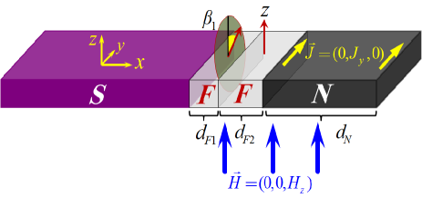
Figure 16: (Color online) Schematic of the proposed $S/F/F/N$ junction. The magnetization orientation of the middle $F$ layer with width $d_{F2}$ is fixed along the $z$ direction. The left $F$ layer, with width $d_{F1}$, has a misaligned magnetization direction corresponding to $\vec{h}_{1}=h_{0}(\cos\pi/4,\sin\pi/4\sin\beta_{1},\cos\beta_{1})$. The normal metal layer has width $d_{N}$. An external magnetic field is applied to the system in the $z$ direction parallel to the interfaces: $\vec{H}=(0,0,H_{z})$. Due to the external magnetic field, a diamagnetic supercurrent flows in the $y$ direction $\vec{J}(x)=(0,J_{y}(x),0)$ and varies along $x$. The junction interfaces lie in the $yz$ plane.

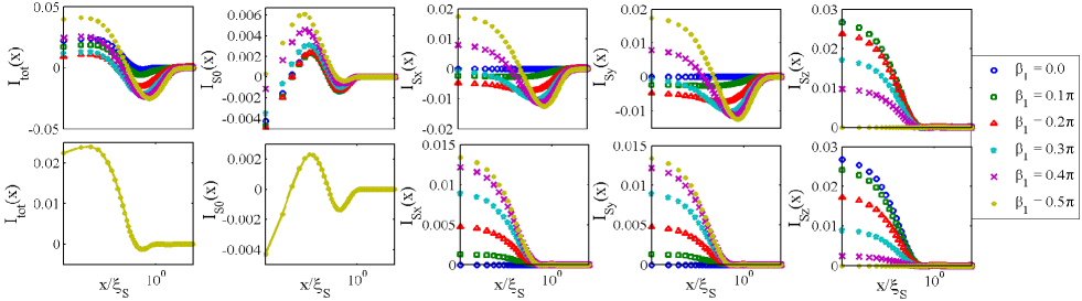
Figure 17: (Color online) Top row: Spatial behavior of the total supercurrent and its components as a function of position inside the $S/F/F/N$ junction for various magnetization orientations in $F_{1}$: $\vec{h}_{1}=h_{0}(\cos\pi/4\sin\beta_{1},\sin\pi/4\sin\beta_{1},\cos\beta_{1})$ for $\beta_{1}=0,0.1\pi,0.2\pi,0.3\pi,0.4\pi$, and $0.5\pi$. The thickness of the left $F$ layer is fixed at $d_{F1}=0.15\xi_{S}$, while the thickness of the right $F$ layer is equal to $d_{F2}=1.85\xi_{S}$. Bottom row: The left and right thicknesses in the $F$ layers are now equal to $d_{F1}=d_{F2}=\xi_{S}$. The sum of $d_{F1}$ and $d_{F2}$ is identical for both cases investigated in the top and bottom rows. The normal layer thickness is also fixed at $2.5\xi_{S}$ in both cases. The logarithmic scales on the $x$-axes permits easier visualization of the long-ranged spatial behavior of the odd-triplet components that have spin projections normal to the $z$ quantization axis.

The magnetization of the left $F$ is determined by a rotation angle $\beta_{1}$ with respect to the $z$ axis ($\vec{h}_{1}=h_{0}(\cos\pi/4\sin\beta_{1},\sin\pi/4\sin\beta_{1},\cos\beta_{1})$) while the magnetization of right $F$ layer is assumed to be fixed along the $z$ axis. The non-superconducting part of the spin-valve is subject to an external magnetic field $\vec{H}$ oriented along the $z$ axis, $H_{z}$. The external magnetic field leads to a diamagnetic supercurrent $\vec{J}$, which depends on $x$ and flows along the $y$ direction [denoted by $J_{y}(x)$] parallel to the interfaces. In the presence of an external magnetic field, we make the usual substitution $\hat{\partial}\rightarrow\vec{\nabla}+e\vec{A}/c$, where $\vec{A}$ is the vector potential, related to the external magnetic field ($\vec{H}$) via $\vec{\nabla}\times\vec{A}=\vec{H}$. In the linear response regimesus1 ; sus2 ; sus3 ; sus4 ; sus5 ; sus6 ; Yokoyama_missner , the supercurrent density can be expressed by:

$${J}_{y}(x)=-J_{0}8ieA_{y}(x)\times$$

$$\int_{0}^{\infty}d\varepsilon\tanh\varepsilon\beta\left\{\mathbb{S}(\varepsilon,x)\mathbb{S}^{\ast}(-\varepsilon,x)-\mathbb{S}(-\varepsilon,x)\mathbb{S}^{\ast}(\varepsilon,x)+\right.$$

$$\left.\mathbb{T}_{x}(-\varepsilon,x)\mathbb{T}_{x}^{\ast}(\varepsilon,x)-\mathbb{T}_{x}(\varepsilon,x)\mathbb{T}_{x}^{\ast}(-\varepsilon,x)+\right.$$

$$\left.\mathbb{T}_{y}(-\varepsilon,x)\mathbb{T}_{y}^{\ast}(\varepsilon,x)-\mathbb{T}_{y}(\varepsilon,x)\mathbb{T}_{y}^{\ast}(-\varepsilon,x)+\right.$$

$$\left.\mathbb{T}_{z}(-\varepsilon,x)\mathbb{T}_{z}^{\ast}(\varepsilon,x)-\mathbb{T}_{z}(\varepsilon,x)\mathbb{T}_{z}^{\ast}(-\varepsilon,x)\right\}.$$ (42)

Strictly speaking, to determine $A_{y}(x)$, it is necessary to solve Maxwell’s equation incorporating the Coulomb gauge in conjunction with the expression for $J_{y}(x)$ and appropriate boundary conditions for $H$ sus1 ; sus2 ; sus3 ; sus4 ; sus5 ; sus6 ; Yokoyama_missner . We have found however that through our extensive numerical investigations, $A_{y}(x)$ is typically a linear function of $x$ and weakly varies with the magnetization alignment, $\beta_{1}$. Therefore, it is the energy and spatial dependence of the Green’s function components in Eq. (IV.6) which governs the supercurrent density. To study the supercurrent behavior, and similar to what was done above for Josephson structures, we separate out the even- and odd-frequency components of the total supercurrent the same as Sec. III.1. We achieve this by first defining $I_{tot}(x)$=$I_{S0}(x)$+$I_{Sx}(x)$+$I_{Sy}(x)$+$I_{Sz}(x)$, where $I_{S0}(x)$, $I_{Sx}(x)$, $I_{Sy}(x)$, and $I_{Sz}(x)$ are given by,

$$I_{S0}(x)=$$

$$\int_{0}^{\infty}d\varepsilon\left\{\mathbb{S}(\varepsilon)\mathbb{S}^{\ast}(-\varepsilon)-\mathbb{S}(-\varepsilon)\mathbb{S}^{\ast}(\varepsilon)\right\}\tanh\varepsilon\beta,$$ (43a)

$$I_{Sx}(x)=$$

$$\int_{0}^{\infty}d\varepsilon\left\{\mathbb{T}_{x}(-\varepsilon)\mathbb{T}_{x}^{\ast}(\varepsilon)-\mathbb{T}_{x}(\varepsilon)\mathbb{T}_{x}^{\ast}(-\varepsilon)\right\}\tanh\varepsilon\beta,$$ (43b)

$$I_{Sy}(x)=$$

$$\int_{0}^{\infty}d\varepsilon\left\{\mathbb{T}_{y}(-\varepsilon)\mathbb{T}_{y}^{\ast}(\varepsilon)-\mathbb{T}_{y}(\varepsilon)\mathbb{T}_{y}^{\ast}(-\varepsilon)\right\}\tanh\varepsilon\beta,$$ (43c)

$$I_{Sz}(x)=$$

$$\int_{0}^{\infty}d\varepsilon\left\{\mathbb{T}_{z}(-\varepsilon)\mathbb{T}_{z}^{\ast}(\varepsilon)-\mathbb{T}_{z}(\varepsilon)\mathbb{T}_{z}^{\ast}(-\varepsilon)\right\}\tanh\varepsilon\beta.$$ (43d)

Also the boundary conditions at the right far end interface of the normal metal should be modified accordingly (see Fig. 12):

$$\partial_{x}(\mp\mathbb{T}_{x}(-\varepsilon)+i\mathbb{T}_{y}(-\varepsilon))=0,$$ (44a)

$$\partial_{x}(\mp\mathbb{S}(-\varepsilon)+\mathbb{T}_{z}(-\varepsilon))=0,$$ (44b)

$$\partial_{x}(\mp\mathbb{T}_{x}^{\ast}(\varepsilon)-i\mathbb{T}_{y}^{\ast}(\varepsilon))=0,$$ (44c)

$$\partial_{x}(\mp\mathbb{S}^{\ast}(\varepsilon)+\mathbb{T}_{z}^{\ast}(\varepsilon))=0.$$ (44d)

Having now established the method in which to determine the spatial behavior of the supercurrent and its decompositions, we present in Fig. 17 our findings for the proposed nanovalve subject to an external magnetic field. Several values of the left magnetization orientation $\beta_{1}$ are investigated (the right $F$ magnetization is fixed along the $z$ axis), corresponding to $\beta_{1}/\pi=0,0.1,0.2,0.3,0.4,0.5$. In the top row, the thickness of the left $F$ layer is much smaller than the thickness of the adjacent $F$ layer: $d_{F1}(=0.15\xi_{S})\ll d_{F2}(=1.85\xi_{S})$. The thickness of the normal metal is of moderate size, set equal to $d_{N}=2.5\xi_{S}$. The total non-superconducting region thus has a thickness of $4.5\xi_{S}$. To demonstrate the long-ranged nature of the spin-1 triplet components $I_{Sx}(x)$ and $I_{Sy}(x)$ in this simple structure with only two magnetic regions with uniform and non-collinear magnetization orientations, we introduce a three dimensional magnetization in the left $F$ region: $\vec{h}_{1}=h_{0}(\cos\pi/4\sin\beta_{1},\sin\pi/4\sin\beta_{1},\cos\beta_{1})$. To clearly show the spatially long-ranged components, we use a logarithmic scale for each $x$-axis. It is seen that the triplet component with zero spin projection on the $z$-axis, $I_{Sz}(x)$, is short-ranged and becomes suppressed at positions approximately greater than $x\sim 0.5\xi_{S}$. This is in drastic contrast to the $I_{Sx}(x)$, and $I_{Sy}(x)$ components, which propagate over the entire non-superconducting region. The singlet component, $I_{S0}(x)$, vanishes around $x\sim\xi_{S}$, which is about half the thickness of the magnetic layers ($d_{F1}+d_{F2}=2\xi_{S}$). Thus, the long-ranged components can strongly influence the total supercurrent, $I_{tot}(x)$, and be the primary source of nonzero supercurrent in the normal metal. These findings are therefore suggestive of an experimentally accessible $S/F/F/N$ spin valve with long-ranged triplet correlations controllable by magnetization rotation in one of the $F$ layers.

It turns out that the the pure spin-1 odd-frequency spin-valve effect is optimal for asymmetric $F$ layer thicknesses. To illustrate this, we consider a symmetric configuration with $d_{F1}=d_{F2}=\xi_{S}$, which ensures the same total thickness of the ferromagnet regions (the normal metal thickness is unchanged at $d_{N}=2.5\xi_{S}$). The results of this configuration are represented in the bottom row of Fig. 17. The total current and its components are plotted as a function of position inside the non-superconducting regions for the same magnetization orientations in the asymmetric case (top row). We find that in contrast to the panels in the top row, the triplet components $I_{Sx}(x)$, $I_{Sy}(x)$, and $I_{Sz}(x)$ are now all short-ranged in the sense that they vanish near $x\sim 0.5\xi_{S}$. In particular, the spin-1 components, $I_{Sx}(x)$, and $I_{Sy}(x)$ do not propagate in $F_{2}$, where the magnetization is orthogonal to the correlations’ spin orientations. The singlet contribution, $I_{S0}(x)$, for both the $d_{F2}\gg d_{F1}$ and $d_{F2}=d_{F1}$ cases shows similar behavior, where it vanishes at around $x\sim\xi_{S}$. This can be understood by noting that the spin-splitting effects of ferromagnetism destroy opposite-spin paring correlations. The total current also vanishes at $x\sim\xi_{S}$ for all magnetization orientations, $\beta_{1}$, in contrast to what was observed in the $d_{F2}\gg d_{F1}$ structure above.

We are now able to compare the behavior of various supercurrent components in the $S$/$F$/$F$/$N$ and the $S$/$F$/$F$/$S$ Josephson structures presented in Sec. III. As seen, our investigations for a wide range of parameters, including misaligned $S$/$F$/$F$/$S$ structures with $d_{F2}\gg d_{F1}$, illustrate localized spin-1 components, $I_{Sx}(x)$, $I_{Sy}(x)$, whereby their spin orientation follows the local magnetization orientation. These components of supercurrent are unable to propagate throughout the bilayer $F$/$F$ junctions where there is a relative orthogonal magnetization. This comparison immediately reveals the efficiency and advantages of a $S$/$F$/$F$/$N$ nanovalve for detecting proximity spin-1 triplet superconducting correlations experimentally. The pure spin-1 triplet diamagnetic response discussed here for the $S$/$F$/$F$/$N$ spin valves might be measured using a local probe such as the density of states or current density. As is well understood, the triplet correlations can alter the induced minigap in the local density of states in the nonsuperconducting regions. For example, the traditional $s$-wave minigap profile can become peaked due to the emergence of triplet correlations which cause a resonance near the Fermi surface. Also, as seen, our findings demonstrate that only spin-1 triplet components of the diamagnetic current survive in the $N$ region if $d_{F2}\gg d_{F1}$, for sufficient magnetization misalignment. Therefore, these results suggest that currents measured experimentally within the $N$ wire for such systems should be comprised of purely equal-spin triplet correlations that are odd-frequency in character.

Therefore, the spin-parameterized technique reveals the spatial profile of the odd and even frequency components of the total supercurrent and provides additional insight into their behaviors. The general three-dimensional approach which we outlined can then be employed for two-dimensional finite-size magnetic/superconducting proximity hybrids with arbitrary magnetization patterns. In this paper we categorized $S$/$F$ hybrids with layered $F$ regions into two classes: configurations hosting supercurrent transport 1) parallel and 2) perpendicular to the $F$/$F$ interface. The one-dimensional structures studied in Sec. III belong to class 2), while the two-dimensional configurations discussed in this section are examples of class 1). For the fairly wide range of configurations considered in this paper, we demonstrated that singlet supercurrent flow “parallel” to uniformly magnetized $F/F$ interfaces can generate substantial long-range triplet supercurrents regardless of the specific configuration and geometry pugach_paral ; Fominov ; al1 . This is of course in stark contrast to their counterparts where the singlet supercurrent flows “perpendicular” to the $F$/$F$ cross sections and fully discussed in Sec. III.

V conclusion

In conclusion, we have employed a quasiclassical method and spin-parameterization technique in both the Usadel equations and associated boundary conditions. This approach provides a suitable computational and analytical framework to pinpoint the spatial behaviors of the decomposed odd and even frequency supercurrent components in layered ferromagnetic junctions. We have studied the transport characteristics of the spin decomposed supercurrent components for two generic scenarios and several experimentally relevant structures: systems with 1) parallel or 2) perpendicular charge supercurrent flow relative to the magnetic interfaces. Two types of finite-size two-dimensional magnetic $S$/$F$/$F$/$S$ Josephson junctions subject to an external magnetic field, and supporting supercurrents flow parallel to the $F$/$F$ interface, are considered. In one type, we assume the $F$/$F$ interface is parallel to the $S$/$F$ interfaces, while in the other type, the $F$/$F$ interface is perpendicular to the $S$/$F$ interfaces. Our studies revealed that when a supercurrent flows parallel to the $F$/$F$ junction, the long-ranged spin-triplet supercurrent will be effectively generated and it will propagate deeply into the ferromagnetic regions independent of junction geometries. This phenomenon is more pronounced when the thickness of ferromagnetic strips are unequal ($d_{F2}\gg d_{F1}$ or $W_{F2}\gg W_{F1}$), depending on the junction type under consideration. This effect disappears when the supercurrent direction is perpendicular to the $F$/$F$ interface. To gain more insight and to have explicit comparisons, we also studied the various aspects of the spin-decomposed supercurrent components in one-dimensional $S/F/F/S$, $S/F/F/F/S$, and $S/Ho/F/Ho/S$ hybrids using the spin-parametrization scheme. We studied the spatial maps of each supercurrent component and found that the total supercurrent is dominated by the long-range triplet component, which also governs the behavior of total supercurrent. Our results demonstrated that structures with inhomogeneous magnetization patterns generate long-ranged supercurrents stronger than their uniform counterparts and that the component of supercurrent corresponding to the rotating magnetization component is long-ranged in such structures. Finally, we proposed an $S$/$F$/$F$/$N$ spin-valve, which represents an experimentally accessible platform to probe the predicted phenomena in the parallel supercurrent transport scenario. We have studied the spatial maps of the singlet and triplet supercurrent components of this spin-valve when subjected to an external magnetic field. Our findings demonstrated that for misaligned magnetizations and different thicknesses of the $F$ layers, $d_{F2}\gg d_{F1}$, a long-ranged odd-triplet component of the supercurrent response arises and populates the adjacent normal metal $N$.

- (1) I. Zutic, J. Fabian, and S.D. Sarma, Rev. Mod. Phys. 76, 323 (2004).
- (2) A.A. Golubov, M.Yu. Kupriyanov, E. Ilichev, Rev. Mod. Phys. 76, 411 (2004).
- (3) A. Buzdin, Rev. Mod. Phys. 77, 935 (2005).
- (4) F.S. Bergeret, A.F. Volkov, K.B. Efetov, Rev. Mod. Phys. 77, 1321 (2005).
- (5) K.B. Efetov, I.A. Garifullin, A.F. Volkov,K. Westerholt, Magnetic Heterostructures,Advances and Perspectives in Spinstructures and Spintransport. ed. by H. Zabel, S.D. Bader, Series. Springer Tracts in Mod. Phys. vol 227 (Springer, New York, 2007), P. 252.
- (6) M. Eschrig, Phys. Today 64, 43 (2011).
- (7) M. Alidoust and K. Halterman, Appl. Phys. Lett. 105, 202601 (2014).
- (8) M. Alidoust and K. Halterman, Phys. Rev. B 89, 195111 (2014).
- (9) K. Halterman, O. T. Valls, and M. Alidoust, Phys. Rev. Lett. 111, 046602 1694 (2013).
- (10) A.M. Bobkov and I.V. Bobkova, Phys. Rev. B 84, 054533 (2011); Phys. Rev. Lett. 108, 197002 (2012).
- (11) A.G. Malshukov, and A. Brataas, Phys. Rev. B86, 094517 (2012).
- (12) L.B. Ioffe, V.B. Geshkenbein, M.V. Feigelman, A.L. Fauchere, and G. Blatter, Nature (London) 398, 679 (1999).
- (13) Y.S. Barash, I.V. Bobkova, and T. Kopp, Phys. Rev. B 66, 140503(R) (2002).
- (14) A. Cottet, T. Kontos, W. Belzig, C. Schonenberger, C. Bruder, Europhys. Lett. 74, 320 (2006).
- (15) B. Crouzy, S. Tollis, and D.A. Ivanov, Phys. Rev. B 76, 134502 (2007).
- (16) Ya.V. Fominov, A.F. Volkov, and K.B. Efetov, Phys. Rev. B 75, 104509 (2007).
- (17) Z. Pajovic, M. Bozovic, Z. Radovic, J. Cayssol, and A. Buzdin, Phys. Rev. B 74, 184509 (2006).
- (18) H. Sellier, C. Baraduc, F. Lefloch, and R. Calemczuk, Phys. Rev. Lett. 92, 257005 (2004).
- (19) N.G. Pugach, M.Yu. Kupriyanov, A.V. Vedyayev, C. Lacroix, E. Goldobin, D. Koelle, R. Kleiner, and A.S. Sidorenko Phys. Rev. B 80, 134516 (2009).
- (20) L.-J. Jin, Y. Wang, L. Wen, G.-Q. Zha, and S.-P. Zhou Physics Letters A 376, 2435 (2012).
- (21) M. Eschrig, J. Kopu, J.C. Cuevas, and G. Schon, Phys. Rev. Lett. 90, 137003 (2003).
- (22) M.N. Baibich, J.M. Broto, A. Fert, F. Nguyen Van Dau, F. Petroff, P. Eitenne, G. Creuzet, A. Friederich, and J. Chazelas, Phys. Rev. Lett. 61, 2472 (1988).
- (23) G. Binasch, P. Grunberg, F. Saurenbach, and W. Zinn, Phys. Rev. B 39, 4828 (1989).
- (24) M. Alidoust, G. Sewell, and J. Linder Phys. Rev. B 85, 144520 (2012).
- (25) M. Alidoust, J. Linder, G. Rashedi, T. Yokoyama, and A. Sodbo, Phys. Rev. B81, 014512 (2010).
- (26) V.I. Zdravkov, J. Kehrle, G. Obermeier, D. Lenk, H.-A. Krug von Nidda, C. Muller, M.Yu. Kupriyanov, A.S. Sidorenko, S. Horn, R. Tidecks, and L.R. Tagirov, Phys. Rev. B 87, 144507 (2013).
- (27) S.V. Bakurskiy, N.V. Klenov, I.I. Soloviev, M.Yu. Kupriyanov, and A.A. Golubov, Phys. Rev. B 88, 144519 (2013).
- (28) Y. Makhlin, G. Schoen, A. Shnirman, Rev. Mod. Phys. 73, 357 (2001).
- (29) V.V. Ryazanov, V.A. Oboznov, A.Yu. Rusanov, A.V. Veretennikov, A.A. Golubov, and J. Aarts, Phys. Rev. Lett. 86, 2427 (2001).
- (30) L.N. Bulaevskii, M.J. Graf, C.D. Batista, and V.G. Kogan, Phys. Rev. B 83, 144526 (2011).
- (31) A.I. Buzdin, L.N. Bulaevskii, S.V. Panyukov, JETP Lett. 35, 178 (1982).
- (32) K. Halterman, and O.T. Valls, Phys. Rev. B 69, 014517 (2004).
- (33) F.S. Bergeret, A.F. Volkov, K.B. Efetov, Phys. Rev. Lett. 86, 4096 (2001).
- (34) Y. Asano, Y. Tanaka, T. Yokoyama, and S. Kashiwaya, Phys. Rev. B 74, 064507 (2006).
- (35) M. Eschrig, T. Lofwander, Nat. Phys. 4, 138 (2008).
- (36) T. Lofwander, T. Champel, J. Durst, M. Eschrig, Phys. Rev. Lett. 95, 187003 (2005).
- (37) T. Kontos, M. Aprili, J. Lesueur, X. Grison, Phys. Rev. Lett. 86, 304 (2001).
- (38) I. Sosnin, H. Cho, V.T. Petrashov, and A.F. Volkov, Phys. Rev. Lett. 96, 157002 (2006).
- (39) K. Halterman, P.H. Barsic, and O.T. Valls Phys. Rev. Lett. 99, 127002 (2007).
- (40) T.S. Khaire, M.A. Khasawneh, W.P. Pratt Jr., N.O. Birge, Phys. Rev. Lett. 104, 137002 (2010).
- (41) R.S. Keizer, S.T.B. Goennenwein, T.M. Klapwijk, G. Miao, G. Xiao and A. Gupta, Nature 439, 825 (2006).
- (42) M. Houzet and A.I. Buzdin, Phys. Rev. B 76, 060504(R) (2007).
- (43) M. Alidoust, and J. Linder, Phys. Rev. B82, 224504 (2010).
- (44) M. Alidoust, K. Halterman, J. Linder, Phys. Rev. B 89, 054508 (2014).
- (45) M. Houzet, A.I. Buzdin, Phys. Rev. B74, 214507 (2006).
- (46) M. Knezevic, L. Trifunovic, Z. Radovic, Phys. Rev. B 85, 094517 (2012).
- (47) L. Trifunovic, Phys. Rev. Lett. 107, 047001 (2011).
- (48) T.Y. Karminskaya, M.Y. Kupriyanov, and A.A. Golubov, JETP Lett. 87, 570 (2008); A.I. Buzdin, A.S. Melnikov, and N.G. Pugach, Phys. Rev. B 83, 144515 (2011).
- (49) S. Hikino and S. Yunoki, Phys. Rev. Lett. 110, 237003 (2013).
- (50) J.W.A. Robinson, J.D.S. Witt, M.G. Blamire, Science 329, 5987 (2010).
- (51) C. Wu, O.T. Valls, and K. Halterman Phys. Rev. Lett. 108, 117005 (2012).
- (52) K. Halterman and O. T. Valls Phys. Rev. B 80, 104502 (2009).
- (53) V.A. Oboznov, V.V. Bolginov, A.K. Feofanov, V.V. Ryazanov, and A.I. Buzdin, Phys. Rev. Lett. 96, 197003 (2006).
- (54) G.A. Ovsyannikov, A.E. Sheyerman, A.V. Shadrin, Yu.V. Kislinskii, K.Y. Constantinian, and A. Kalabukhov JETP Letters 97, 145 (2013)
- (55) T.Yu. Karminskaya, A.A. Golubov, and M.Yu. Kupriyanov, Phys. Rev. B 84, 064531 (2011).
- (56) C. Wu, O.T. Valls, and K. Halterman, Phys. Rev. B 86, 014523 (2012).
- (57) A.S. Melnikov, A.V. Samokhvalov, S.M. Kuznetsova, and A.I. Buzdin, Phys. Rev. Lett. 109, 237006 (2012).
- (58) S. Oh, D. Youm and M.R. Beasley, Appl. Phys. Lett. 71, 2376 (1997).
- (59) Y.V. Fominov et al., JETP Lett. 91, 308 (2010).
- (60) P.V. Leksin, N.N. Garifyanov, I.A. Garifullin, Ya.V. Fominov, J. Schumann, Y. Krupskaya, V. Kataev, O.G. Schmidt, and B. B chner, Phys. Rev. Lett. 109, 057005 (2012).
- (61) P.V. Leksin, N.N. Garifyanov, I.A. Garifullin, J. Schumann, V. Kataev, O.G. Schmidt, and B. B chner, Phys. Rev. Lett. 106, 067005 (2011).
- (62) P.V. Leksin, N.N. Garifyanov, I.A. Garifullin, J. Schumann, V. Kataev, O.G. Schmidt, and B. B chner, Phys. Rev. B 85, 024502 (2012).
- (63) B. Li, N. Roschewsky, B.A. Assaf, M. Eich, M. Epstein-Martin, D. Heiman, M. M nzenberg, and J. S. Moodera, Phys. Rev. Lett. 110, 097001 (2013).
- (64) P.V. Leksin, N.N. Garifyanov, I.A. Garifullin, J. Schumann, H. Vinzelberg, V. Kataev, R. Klingeler, O.G. Schmidt and B. B chner, Appl. Phys. Lett. 97, 102505 (2010).
- (65) A.A. Jara, C. Safranski, I.N. Krivorotov, C. Wu, A.N. Malmi-Kakkada, O.T. Valls, and K. Halterman, Phys. Rev. B89, 184502 (2014).
- (66) M.G. Flokstra, T.C.Cunningham, J. Kim, N. Satchell, G. Burnell, S.J. Bending, P.J. Curran, S.J. Langridge, C. Kinane, J.F.K. Cooper, N. Pugach, M. Eschrig, S.L. Lee, arXiv:1404.2950.
- (67) V. Braude, Yu.V. Nazarov, Phys. Rev. Lett. 98, 077003 (2007).
- (68) F.S. Bergeret and J.C. Cuevas, J. Low Temp. Phys., 153 304 (2008).
- (69) J.M. Rowell, Phys. Rev. Lett. 11, 200 (1963).
- (70) B.D. Josephson, Phys. Lett. 1, 251 (1962).
- (71) J.C. Cuevas and F.S. Bergeret, Phys. Rev. Lett., 99 217002 (2007).
- (72) M. Alidoust, G. Sewell, and J. Linder, Phys. Rev. Lett. 108, 037001 (2012).
- (73) M. Alidoust, and J. Linder, Phys. Rev. B 87, 060503(R) (2013).
- (74) U. Ledermann, A.L. Fauche‘re, and G. Blatter, Phys. Rev. B 59, R9027 (1999).
- (75) K. Usadel, Phys. Rev. Lett. 25, 507 (1970); A.I. Larkin and Y.N. Ovchinnikov, in Nonequilibrium Superconductivity, edited by D. Langenberg and A. Larkin (Elsevier, Amesterdam, 1986), P. 493.
- (76) J.P. Morten, M.S. thesis, Norwegian University of Science and Technology, 2003.
- (77) W. Belzig, F.K. Wilhelm, C. Bruder, G. Sch n, A. D.Zaikin, Superlattices and Microstructures, Vol. 25, Iss. 5 6, Pg. 1251 (1999).
- (78) A. V. Zaitsev, Zh. Eksp. Teor. Fiz. 86, 1742 (1984) (Sov. Phys. JETP 59, 1015 (1984); M. Y. Kuprianov et al., Sov. Phys. JETP 67, 1163 (1988).
- (79) L. Angers, F. Chiodi, G. Montambaux, M. Ferrier, S. Guèron, H. Bouchiat, and J.C. Cuevas, Phys. Rev. B 77, 165408 (2008).
- (80) F. Chiodi, M. Ferrier, Guèron, J.C. Cuevas, G. Montambaux, F. Fortuna, A. Kasumov, H. Bouchiat, Phys. Rev. B 86, 064510 (2012).
- (81) J.R. Clem, Phys. Rev. B 81, 144515 (2010).
- (82) A.F. Volkov and K.B. Efetov, Phys. Rev. B 81, 144522 (2010).
- (83) T. Champel, M. Eschrig, Phys. Rev. B 72, 054523 (2005).
- (84) M. Eschrig, T. Lofwander, T. Champel, J.C. Cuevas, J. Kopu, G. Schon, J. Low Temp. Phys. 147, 457, (2007).
- (85) G.B. Halsz, J.W.A. Robinson, J.F. Annett, and M.G. Blamire, Phys. Rev. B 79, 224505 (2009)
- (86) D. Fritsch and J.F. Annett, New J. Phys. 16, 055005 (2014).
- (87) H. Suderow, I. Guillamon, J.G. Rodrigo, S. Vieira, arXiv:1403.5514.
- (88) A.A. Abrikosov, Fundamentals of the Theory of Metals (North-Holland, Amsterdam, 1988).
- (89) T. Yamashita, L. Rindereer, J. Low Temp. Phys. 21, 153 (1975).
- (90) A.A. Abrikosov, Sov. Phys. JETP 5, 1174 (1957).
- (91) M. Tinkham, Introduction to Superconductivity (McGraw-Hill, New York, 1996).
- (92) T. Lofwander, T. Champel, M. Eschrig, Phys. Rev. B 75, 014512 (2007).
- (93) Higashitani and K. Nagai, Physica B 194, 1385 (1994).
- (94) W. Belzig, C. Bruder, and G. Schön, Phys. Rev. B 53, 5727 (1996).
- (95) P. Visani et al., Phys. Rev. Lett. 65, 1514 (1990).
- (96) F. Bernd, Muller-Allinger and A. Celia Mota, Phys. Rev. Lett. 84, 3161 (2000).
- (97) F. Bernd Muller-Allinger and A. Celia Mota, Phys. Rev. B 62, 6120 (2000).
- (98) C. Bruder and Y. Imry, Phys. Rev. Lett. 80, 5782 (1998).
- (99) T. Yokoyama, Y. Tanaka, and N. Nagaosa, Phys. Rev. Lett. 106, 246601 (2011).
- (100) K. Halterman, O. T. Valls, and M. Alidoust, Phys. Rev. Lett. 111, 046602 1694 (2013).