Chiral universality class of the normal-superconducting and the exciton condensation transition on the surface of topological insulator

Abstract

New two dimensional systems like surface of topological insulator and graphene offer a possibility to experimentally investigate situations considered ”exotic” just a decade ago. One of those is the quantum phase transition of the ”chiral” type in electronic systems with relativistic spectrum. Phonon mediated (”conventional”) pairing in the Dirac semimetal appearing on the surface of topological insulator leads to transition into a chiral superconducting state, while exciton condensation in these gapless systems has been envisioned long time ago in the physics of the narrow band semiconductors. Starting from the microscopic Dirac Hamiltonian with local attraction or repulsion, the BCS type gaussian approximation is developed in the framework of functional integrals. It is shown that due to an ”ultra-relativistic” dispersion relation there is a quantum critical point governing the zero temperature transition to a superconducting or the exciton condensed state. The quantum transitions that have critical exponents very different from the conventional ones. They belong to the chiral universality class. We discuss the application of these results to recent experiments in which surface superconductivity was found in topological insulators and estimate feasibility of the phonon pairing.

I Introduction

Topological insulator (TI) is a novel state of matter in materials with strong spin - orbit interactions that create topologically protected surface states Zhang . The electrons (holes) in these states have a linear dispersion relation, see Fig. 1, and can be described approximately by a (pseudo) relativistic two dimensional (2D) Hamiltonian. The system realizes an ”ultra-relativistic” 2D electron or hole conducting liquid along with much better studied grapheneKatsnelson , a 2D one layers sheet of carbon atoms that became a paradigms example of the Dirac semi-metal. In the context of graphene certain quantum phase transitions were theoretically contemplated. The superconductivity in graphene has been repeatedly consideredsupergraphene , however despite great experimental efforts was never achieved. The 2D dimensional phonons seem to be unable to overcome strong Coulomb repulsion in order to create a Cooper pair. The same can be said about attempts to achieve exciton condensate in graphene that was proposedKhveshchenko ; Gamayun even before its discovery. Apparently the repulsion is not strong enough either to create stable electron - hole bound statesgraphenechiral . The surface of topological insulator therefore became a prime candidate to realize the quantum transitions.

It is known for a long time that similar 2D and quasi-2D metallic systems like the surface metal on twin planes Shapiro , layered materials (strongly anisotropic high $T_{c}$ cupratesWen or organic superconductorsorganic ) may develop 2D (surface) superconductivity. This phenomenon became known as ”localized superconductivity”Buzdin . Since best studied TIs possess a quite standard phonon spectrum phononexp , it was predicted recently DasSarma ; Li14 that they become superconducting. The predicted critical temperature of order of $1K$ is rather low (despite a fortunate suppression of the Coulomb repulsion due to a large dielectric constant $\varepsilon\sim 50$), the nature of the ”normal” state (so-called 2D Weyl semi-metal) might make the superconducting properties of the system unusual. The ultra-relativistic nature manifests itself mostly when the Weyl cone is very close to the Fermi surface. Especially interesting is the case (that actually was originally predicted for the [111] surface of $Bi_{2}Te_{3}$ and $Bi_{2}Se_{3}$Zhang1 ) when the chemical potential coincides with the Dirac point. Although subsequent ARPES experimentsZhang show the location of the cone of surface states order tenths of $eV$ off the Fermi surface; there are experimental means to shift the chemical potential, for example by the bias voltage bias .

Unlike the more customary poor 2D metals with several small pockets of electrons/holes on the Fermi surface (in semiconductor systems or even some high $T_{c}$ materialsWen ), the electron gas TI has two peculiarities especially important when pairing is contemplated. The first is the bipolar nature of the Dirac spectrum: there is no energy gap between the upper and lower cones. The second is that  the spin degree of freedom is a major player in the quasiparticle dynamics. This degree of freedom determines the pairing channel. The pairing channel problem was studied theoretically on the level of the Bogoliubov-deGennes equation Herbut . Both $s$-wave and $p$-wave are possible and compete due to the breaking of the bulk inversion symmetry by the surface. Various pairing interactions were considered to calculate the DOS measured in $Cu_{x}Bi_{2}Se_{3}$ using self-consistent analysis Sato . As mentioned above the most intriguing case is that of the small chemical potential that has not been addressed microscopically. It turns out that it is governed by a quantum critical point (QCP)Sachdev .

The concept of QCP at zero temperature and varying doping constitutes a very useful language for describing the microscopic origin of superconductivity in high $T_{c}$ cuprates and other ”unconventional” superconductorsWen . Superconducting transitions generally belong to the $U\left(1\right)$ class of second order phase transitionsHerbutbook , however it was pointed out a long time agoRosenstein that, if the normal state dispersion relation is ”ultra-relativistic”, the transition at zero temperature as function of parameters like the pairing interaction strength is qualitatively distinct and belongs to chiral universality classes classified in ref. Gat . The term ”chiral” appears following the corresponding discussion of the well studied both theoretically and experimentally chiral symmetry breaking transition in Quantum Chromodynamics. Attempts to experimentally identify second order transitions governed by QCP in condensed matter included quantum magnets Sachdev , superconductor - insulator transitionsSCinsulator and more recently exciton condensate in grapheneKatsnelson ; CastroNeto and other Dirac semi - metals including TI. In the last two cases the broken symmetry is also often termed ”chiral”.

Exciton condensation is a very old concept in low dimensional narrow gap semiconductor physics. The best-studied exciton condensate is the quantum Hall bilayer at half-filled Landau levelsQHE . Here ingenious methods had been developed to separately contact the two layers so that one can directly probe the order parameter via counterflow superfluidity along the layers and tunneling between the layers. The same idea was extended to bilayer graphene and recently to TIexcitonTI .

In addition Dirac semimetal was realized in cold atom systemcold (following the realization in 2D known as the ”synthetic graphene”). Interestingly the sign and strength of the interaction can be controlled. The Dirac semimetal in optically trapped cold atom systems cold is well suited to study this fascinating phenomenon. The Dirac semimetal in optically trapped cold atomscold offers a well controllable system in which this phenomenon occurs both for repulsive interaction (chiral symmetry breaking) and the attractive one (superconductivity).

In this paper the quantum phase transitions in Dirac semimetal due to local interactions both attractive (superconductivity) and repulsive (exciton condensation) are studied with emphasis on their distinct criticality. The critical exponents belong to chiral universality classes that are identified.

In Section II the general framework that allows to study the surface superconductivity and exciton condensation in general Dirac semi-metal (TI, not necessarily time reversal and reflection invariant or some other of the numerous systems being identified recently) with a general local interaction is presented. The local coupling strength $g$, chemical potential $\mu$ and temperature $T$ will be kept general ($g$ is negative for repulsion leading to the exciton condensation or positive leading to superconductivity). Since the symmetry analysis is crucial, we first discuss the space and spin rotations. In Section III we concentrate on the simplest time reversal and reflection invariant Dirac model and identify its spontaneous symmetry breaking patterns. In Section IV the phase diagram for $g>0$ is obtained for arbitrary temperature $T$ and chemical potential much smaller than the Debye energy $T_{D}$. The latter condition is the main difference from the conventional BCS model in which $\mu>>T_{D}$. A quantum critical point at $T=\mu=0$ when the coupling strength $g$ reaches a critical value $g_{c}$ dependent on the cutoff parameter $T_{D}$. We concentrate on properties of the superconducting state in a part of the phase diagram that is dominated by the QCP. Various critical exponents are obtained. In particular, the coupling strength dependence of the coherence length is $\xi\propto\left(g-g_{c}\right)^{-\nu}$ with $\nu=1$ , the order parameter scales as $\Delta\propto\left(g-g_{c}\right)^{\beta}$, $\beta=1$. For the repulsion similar transition occurs in the exciton channel in Section V. The critical exponents beyond mean field and experimental feasibility of superconductivity are discussed in Section VI.

II Generalized mean field approximation for local four - Fermi interactions

II.1 Hamiltonian and the partition function

We consider the second quantized electron Hamiltonian via four-Fermi local coupling of strength $g$

$$H=\int d^{2}r\psi_{\alpha}^{\dagger}\left(\mathbf{r}\right)K_{\alpha\beta}\psi_{\beta}\left(\mathbf{r}\right)\mathbf{-}\frac{g}{2}\psi_{\alpha}^{\dagger}\left(\mathbf{r}\right)\psi_{\beta}^{\dagger}\left(\mathbf{r}\right)\psi_{\beta}\left(\mathbf{r}\right)\psi_{\alpha}\left(\mathbf{r}\right)\text{;}$$

$$K_{\alpha\beta}\left(\mathbf{\nabla}\right)=\mathcal{E}_{\alpha\beta}\left(\mathbf{\nabla}\right)-\mu\delta_{\alpha\beta}\text{,}$$ (1)

where space is two dimensional, $\mathbf{r=}\left\{x,y\right\}$ and $\mu$ is the chemical potential. The precise definition of the relevant ”single” electronic excitations $\mathcal{E}_{\alpha\beta}\left(\mathbf{\nabla}\right)$ will be dependent on the specific model considered and is specified below. The index $\alpha$ of the spinors $\psi$ refers to valley/spin degrees of freedom. The partition function is

$$Z=\mathrm{Tr}\text{ }e^{-H/T}=\int D\psi^{+}D\psi e^{-S\left[\psi_{\alpha}^{+}\mathbf{,}\psi_{\alpha}\right]}\text{,}$$ (2)

with measure defined by independent Grassmann variables $D\psi^{+}=\underset{\alpha}{\Pi}d\psi_{\alpha}^{+},D\psi=\underset{\alpha}{\Pi}d\psi_{\alpha}$. The Matsubara action reads:

$$S\left[\psi^{+}\mathbf{,}\psi\right] = \int_{0}^{1/T}d\tau\int_{r}\psi_{\alpha}^{+}\left(\tau,\mathbf{r}\right)\left(\partial_{\tau}+K_{\alpha\beta}\right)\psi_{\beta}\left(\tau,\mathbf{r}\right)$$ (3)

$$\mathbf{-}\frac{g}{2}\psi_{\alpha}^{+}\left(\tau,\mathbf{r}\right)\psi_{\beta}^{+}\left(\tau,\mathbf{r}\right)\psi_{\beta}\left(\tau,\mathbf{r}\right)\psi_{\alpha}\left(\tau,\mathbf{r}\right)\text{,}$$

with the anti-periodic conditions,

$$\psi_{\alpha}^{+}\left(\tau,\mathbf{r}\right) = -\psi_{\alpha}^{+}\left(\tau+1/T,\mathbf{r}\right),$$ (4)

$$\psi_{\alpha}\left(\tau,\mathbf{r}\right) = -\psi_{\alpha}\left(\tau+1/T,\mathbf{r}\right)\text{.}$$

The local interaction term is not the most general one, but generalization to more ”exotic” local cases (inter-valleyFu the exchange spin - spin couplingRosenstein15 ) is quite straightforward.

The normal and anomalous Green’s functions (consistent with definition in ref.AGD ) are:

$$\left\langle T\psi_{\alpha}\left(X\right)\psi_{\beta}^{+}\left(X^{\prime}\right)\right\rangle = -G_{\alpha\beta}\left(X\mathbf{;}X^{\prime}\right)\text{;}$$

$$\left\langle T\psi_{\alpha}\left(X\right)\psi_{\beta}\left(X^{\prime}\right)\right\rangle = F_{\alpha\beta}\left(X\mathbf{;}X^{\prime}\right)\text{;}$$ (5)

$$\left\langle T\psi_{\alpha}^{+}\left(X\right)\psi_{\beta}^{+}\left(X^{\prime}\right)\right\rangle = F_{\alpha\beta}^{+}\left(X\mathbf{;}X^{\prime}\right)\text{,}$$

where $X=\left(\mathbf{r,}\tau\right)$, $X^{\prime}=\left(\mathbf{r}^{\prime},\tau^{\prime}\right)$. For simplicity, we denote $\left\langle\psi_{\alpha}\left(X\right)\right\rangle$ as $\psi_{\alpha}\left(X\right)$, and drop the time ordering operation $T$ in correlators. For example, $\left\langle\psi_{\alpha}\left(X\right)\psi_{\beta}\left(X^{\prime}\right)\right\rangle$ stands for $\left\langle T\psi_{\alpha}\left(X\right)\psi_{\beta}\left(X^{\prime}\right)\right\rangle$. Their expressions via partition function, Eq.(3), are given in Appendix A.

II.2 Space and spin rotations symmetries

Generally a system may be invariant under both the space rotation and the spin rotation separately. Certain valley symmetries are generally present. In Weyl semimetals, the action is typically only invariant under the combined space rotation and spin/valley rotation. The space rotation, $\mathbf{r}^{\prime}=\Lambda\mathbf{r}$, acts on a generalized spinor field as:

$$\psi_{\alpha}^{\prime}\left(\mathbf{r}^{\prime},\tau\right) = S\left(\Lambda\right)_{\alpha\alpha^{\prime}}\psi_{\alpha^{\prime}}\left(\mathbf{r},\tau\right),$$ (6)

$$\psi_{\beta}^{\prime+}\left(\mathbf{r}^{\prime},\tau\right) = \psi_{\beta^{\prime}}^{+}\left(\mathbf{r},\tau\right)S\left(\Lambda\right)_{\beta^{\prime}\beta}^{\dagger}\text{.}$$

The invariance of the action under the transformation, the correlators satisfy:

$$G_{\alpha\beta}\left(X_{1},X_{2}\right) = S\left(\Lambda\right)_{\alpha\alpha^{\prime}}G_{\alpha^{\prime}\beta^{\prime}}\left(X_{1},X_{2}\right)S\left(\Lambda\right)_{\beta^{\prime}\beta}^{\dagger};$$

$$F_{\alpha\beta}\left(X_{1},X_{2}\right) = S\left(\Lambda\right)_{\alpha\alpha^{\prime}}F_{\alpha^{\prime}\beta^{\prime}}\left(X_{1},X_{2}\right)S\left(\Lambda\right)_{\beta^{\prime}\beta}^{t}$$ (7)

or in the matrix form:

$$G\left(X_{1},X_{2}\right) = S\left(\Lambda\right)G\left(X_{1},X_{2}\right)S\left(\Lambda\right)^{\dagger},$$ (8)

$$F\left(X_{1},X_{2}\right) = S\left(\Lambda\right)F\left(X_{1},X_{2}\right)S\left(\Lambda\right)^{t}$$

Assuming that the ground state is homogeneous, $G\left(X,X\right)\equiv G_{c}$ and $F\left(X,X\right)\equiv g^{-1}\Delta$ are constant matrices satisfying

$$G_{c}=S\left(\Lambda\right)G_{c}S\left(\Lambda\right)^{+},\Delta=S\left(\Lambda\right)\Delta S\left(\Lambda\right)^{t}\text{.}$$ (9)

Let $\Sigma$ be generator of $S\left(\Lambda\right)$. Then

$$\left[\Sigma,G_{c}\right]=0,\Sigma\Delta+\Delta\Sigma^{t}=0$$ (10)

$G_{c}$ and $\Delta$ also satisfy the following equations:

$$G_{c}^{+}=G_{c},\Delta^{t}=-\Delta\text{.}$$ (11)

In superconductor $G_{\alpha\beta}^{c}=n_{c}\delta_{\alpha\beta}$ and leads within the BCS approximation just to renormalization of the chemical potential. Therefore we finally obtain the Gor’kov equations,

$$\left(-\partial_{\tau}\delta_{\alpha\beta}-K_{\alpha\beta}\left(\mathbf{\nabla}\right)\right)G_{\beta\gamma}\left(X,X^{\prime}\right)\mathbf{-}g\times$$

$$F_{\beta\alpha}\left(X,X\right)F_{\beta\gamma}^{+}\left(X,X^{\prime}\right)=\delta\left(X-X^{\prime}\right)\delta_{\alpha\gamma};$$ (12)

$$\left(\partial_{\tau}\delta_{\alpha\beta}-K_{\beta\alpha}\left(-\mathbf{\nabla}\right)\right)F_{\beta\gamma}^{+}\left(X,X^{\prime}\right)-$$

$$gF_{\alpha\beta}^{+}\left(X,X\right)G_{\beta\gamma}\left(X,X^{\prime}\right)=0\text{.}$$

We will also discuss the non-superconducting state like the exciton condensate with opposite bulk properties, $G_{\alpha\beta}^{c}\left(X,X\right)\neq n_{c}\delta_{\alpha\beta}$, $F_{\alpha\beta}\left(X;X^{\prime}\right)=0$. In this case the Dyson - Schwinger form is more convenient. The gap equation can be recasted (see Appendix A) in matrix form as

$$G^{-1}=G_{0}^{-1}+g\delta\left(X-X^{\prime}\right)G_{c}^{\prime}\text{,}$$ (13)

where $G_{\alpha\beta}^{\prime}$ is the traceless part of $G_{\alpha\beta}$,

$$G_{\alpha\beta}^{\prime}\left(X;X^{\prime}\right)=-\left\langle\psi_{\alpha}\left(X\right)\psi_{\beta}^{+}\left(X^{\prime}\right)\right\rangle_{c}+$$ (14)

$$\frac{1}{4}\delta_{\alpha\beta}\sum\left\langle\psi_{\gamma}\left(X\right)\psi_{\gamma}^{+}\left(X^{\prime}\right)\right\rangle_{c},$$

with renormalized chemical potential taking case of the trace as in superconductor.

The Matsubara Green’s functions ($\tau$ is the Matsubara time) for uniform superconducting states can be expressed via Fourier transforms,

$$G_{\alpha\beta}\left(\mathbf{r},\tau;\mathbf{r}^{\prime},\tau^{\prime}\right)=\frac{T}{\left(2\pi\right)^{D}}\int d^{D}\mathbf{k}\times$$

$$e^{i\mathbf{k\cdot}\left(\mathbf{r-r}^{\prime}\right)}\sum_{n}e^{-i\omega_{n}\left(\tau-\tau^{\prime}\right)}G_{\alpha\beta}\left(\mathbf{k,}\omega_{n}\right)\text{;}$$ (15)

$$F_{\alpha\beta}^{\dagger}\left(\mathbf{r},\tau;\mathbf{r}^{\prime},\tau^{\prime}\right)=\frac{T}{\left(2\pi\right)^{D}}\int d^{D}\mathbf{k}\times$$

$$e^{i\mathbf{k\cdot}\left(\mathbf{r-r}^{\prime}\right)}\sum_{n}e^{-i\omega_{n}\left(\tau-\tau^{\prime}\right)}F_{\alpha\beta}^{\dagger}\left(\mathbf{k,}\omega_{n}\right)\text{,}$$

where $\omega=\pi T\left(2n+1\right)$ is the Matsubara Fermionic frequency. The Matsubara Green’s functions in Fourier forms can simplify the calculation significantly.

General formulaAGD obtained in Appendix B for the energy of the superconducting state reads:

$$\frac{d\Omega}{d\left(g^{-1}\right)}\mathcal{=}\frac{V}{2}\text{Tr}\left(\Delta\Delta^{{\dagger}}\right)$$ (16)

while for chiral symmetry breaking (exciton condensation) states the gaussian energy isCJT

$$\Omega=-\text{Tr}\{-\ln G+[G_{0}^{-1}G-1]\}+\frac{g}{2}\text{Tr}G_{c}G_{c}^{{\dagger}}\ \text{.}$$ (17)

III The Dirac model and its symmetries

III.1 Hamiltonian of the time reversal invariant TI with local interaction.

Electrons on the surface of a TI perpendicular to $z$ axis are described by a Pauli spinors $\psi\left(\mathbf{r}\right)$, where the upper plane, $\mathbf{r}=\left\{x,y\right\}$. In principle there are multiple valleys. The case of just one valley describing surface of the topological insulator like $Bi_{2}Te_{3}$ were considered in Zhang ; Herbut ; Li14 . It breaks time reversal invariance and does not allow chiral symmetry breaking, so here we consider the simplest case of multiple valleys: the Dirac model in which chiralities of the two Weyl modes are opposite described by field operators $\psi_{fs}\left(\mathbf{r}\right)$, where $f=L,R$ are the valley index (pseudospin) for the left/right chirality bands with spin projections taking the values $s=\uparrow,\downarrow$ with respect to, for example, $z$ axis. To use the Dirac (”pseudo-relativistic”) notations, these are combined into a four component bi-spinor creation operator, $\psi^{\dagger}=\left(\psi_{L\uparrow}^{\dagger},\psi_{L\downarrow}^{\dagger},\psi_{R\uparrow}^{\dagger},\psi_{R\downarrow}^{\dagger}\right)$, whose index $\gamma=\left\{f,s\right\}$ takes four values. The non-interacting massless Hamiltonian with Fermi velocity $v_{F}$ and linear dispersion relation, see Fig.1, readsWang13 ,

$$\mathcal{E}_{\gamma\delta}=-i\hbar v_{F}\nabla^{i}\alpha_{\gamma\delta}^{i}\text{,}$$ (18)

where two $4\times 4$ matrices, $i=x,y$,

$$\mathbf{\alpha}=\left(\begin{array}[]{cc}\mathbf{\sigma}&0\\ 0&-\mathbf{\sigma}\end{array}\right)\text{,}$$ (19)

are presented in the block form via Pauli matrices $\mathbf{\sigma}$. They are related to the Dirac $\mathbf{\gamma}$ matrices (in the chiral representation, sometimes termed ”spinor”) by $\ \mathbf{\alpha}=\beta\mathbf{\gamma}$ with

$$\beta=\left(\begin{array}[]{cc}0&\mathbf{1}\\ \mathbf{1}&0\end{array}\right)\text{.}$$ (20)

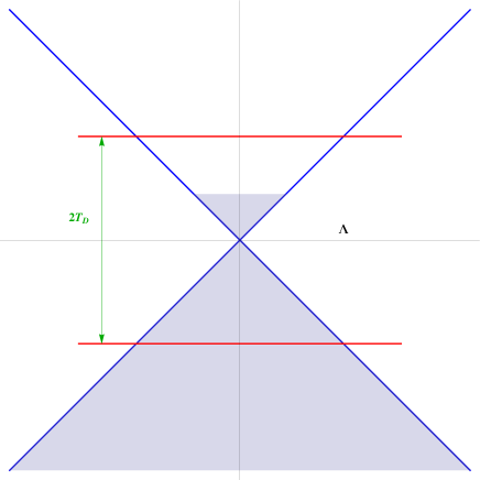
Figure 1: Schematic picture of the band reconstruction of Weyl semi-metal.

The noninteracting Hamiltonian in these notations reads:

$$K=\int_{\mathbf{r}}\psi^{\dagger}\left\{-i\hbar v_{F}\beta\gamma\cdot\mathbf{\nabla}-\mu\right\}\psi\text{.}$$ (21)

The Matsubara action, Eq.(3), is conveniently written in pesudo-relativistic notations with $\overline{\psi}=\psi^{+}\gamma_{0}$ with (Euclidean) $\gamma_{0}=i\beta$:

$$S = \int_{\tau=0}^{1/T}\int_{\mathbf{r}}\left\{-\overline{\psi}\left(\gamma_{0}\partial_{\tau}+\hbar v_{F}\gamma\cdot\mathbf{\nabla-}\mu\gamma_{0}\right)\psi+\right.$$

$$\left.\frac{g}{2}\overline{\psi}\gamma_{0}\psi\overline{\psi}\gamma_{0}\psi\right\}\text{.}$$

Since our focus is on symmetry and its spontaneous breaking, let us review known discrete and continuous symmetries.

III.2 Continuous symmetries

Symmetries of the 2D Dirac model with local interactions Eqs.(1,18) were thoroughly discussed in relation to grapheneGusynin . They include parity, time reversal and the discrete chiral (flavor) transformation: $\psi\rightarrow\gamma_{5}\psi;\overline{\psi}\rightarrow-\overline{\psi}\gamma_{5}$, where $\gamma_{5}=\gamma_{0}\gamma_{1}\gamma_{2}\gamma_{3}=\gamma_{5}^{\dagger}$. Spontaneous breaking of this symmetry has been comprehensively investigated in the context of grapheneGusynin and will not be stressed here. There are also three continuous symmetries that in principle can lead to ordered phase with massless Goldstone bosons (order parameter waves). The first is the usual electric charge $U\left(1\right)$, $\psi\rightarrow e^{i\chi}\psi$, that is spontaneously broken in a superconducting state studied in next section. In addition there is the ”chiral” flavour rotations $SU\left(2\right)$ that play an important role in exciton condensation that will be addressed in section V.

III.2.1 Space time symmetries: just Aphelian space rotation combined with spin (pseudospin) rotation

Unlike the non-interacting model the pseudorelativistic 2+1 dimensional Lorentz invariance is explicitly broken by the static interaction Eq.(1), so that only 2D rotations accompanied by the (pseudo) spin rotation already described in Section II with spin $\Sigma$ operator,

$$\Sigma\mathbf{=}\left(\begin{array}[]{cc}\sigma_{z}&0\\ 0&\sigma_{z}\end{array}\right)=\gamma_{1}\gamma_{2}\text{,}$$ (23)

remain a symmetry. The conserved quantity is the abelian angular momentum

$$J=\int_{\mathbf{r}}\psi^{\dagger}\left(\mathbf{r}\right)\left\{i\varepsilon_{ij}r_{i}\nabla_{j}+\frac{1}{2}\mathbf{\Sigma}\right\}\psi\left(\mathbf{r}\right)\text{.}$$ (24)

The second part is referred to as the spin rotation, $S=\frac{1}{2}\int\psi^{\dagger}\mathbf{\Sigma}\psi$.

III.2.2 Electric charge $U\left(1\right)$

The usual electric charge $U\left(1\right)$ with conserved electric charge:

$$Q=\int_{\mathbf{r}}\psi^{\dagger}\left(\mathbf{r}\right)\psi\left(\mathbf{r}\right)=\int_{\mathbf{r}}\rho\left(\mathbf{r}\right)\text{.}$$ (25)

Action Eq.(III.1) is invariant under the phase (global gauge) transformation, $\psi\rightarrow e^{i\chi}\psi$

III.2.3 Flavour (chiral or valley) $SU(2)$

It was noticed early on in relation to grapheneGusynin that there is flavour $SU\left(2\right)$ symmetry. It is shown in Appendix C that quantities

$$Q_{i}=\int_{\mathbf{r}}\psi^{\dagger}\left(\mathbf{r}\right)T_{i}\psi\left(\mathbf{r}\right),$$ (26)

commute with Hamiltonian and thus are conserved quantities.The generator matrices,

$$T_{1}=\frac{i}{2}\gamma_{3},T_{2}=\frac{1}{2}\gamma_{5},T_{3}=\frac{1}{2}\gamma_{3}\gamma_{5}\text{,}$$ (27)

($\gamma_{5}=\gamma_{0}\gamma_{1}\gamma_{2}\gamma_{3}$) constitute a nonrelativistic $SU\left(2\right)$ algebra:

$$\left[T_{i},T_{j}\right]=i\varepsilon_{ijk}T_{k}\text{.}$$ (28)

A discrete chiral symmetry is just the chiral rotation by angle $\pi$.The action Eq.(III.1) is invariant under infinitesimal transformation, $\delta\psi=iT_{i}\psi;$  $\delta\overline{\psi}=i\overline{\psi}\gamma_{0}T_{i}\gamma_{0}$. All three continuous symmetries commute??(meaning charge, Flavour, and space time symmetry commute).

III.3 Spontaneously broken electric charge $U\left(1\right)$ symmetry phases: superconducting pairing channels

Due to locality of the dominant interactions, the superconducting order parameter is local,

$$O=\int_{\mathbf{r}}\psi_{\alpha}^{\dagger}\left(\mathbf{r}\right)M_{\alpha\beta}\psi_{\beta}^{\dagger}\left(\mathbf{r}\right),$$ (29)

where the constant matrix $M$ should be a $4\times 4$ antisymmetric matrix. Due to the rotation symmetry they transform covariantly under infinitesimal rotations generated by the spin $\Sigma$ operator Eq.(23).

Out of 16 matrices of the four dimensional Clifford algebra six are antisymmetric. We will not consider rather exotic phases in which in addition to the charge $U\left(1\right)$ symmetry neither the 2D rotations or the $SU\left(2\right)$ chiral transformations are spontaneously broken. Therefore superconducting order parameter is invariant under the remaining symmetries: $\left[O,J\right]=\left[O,Q_{i}\right]=0$. Namely it is invariant under the $SU\left(2\right)$ and is either scalar or pseudoscalar under rotations. The requirement of invariance expressed using Eq.(23) takes a form:

$$\left[O,J\right] = \int_{\mathbf{r,r}^{\prime}}\left[\psi_{\alpha}^{\dagger}\left(\mathbf{r}\right)M_{\alpha\beta}\psi_{\beta}^{\dagger}\left(\mathbf{r}\right)\right.,$$

$$\left.\psi_{\gamma}^{\dagger}\left(\mathbf{r}^{\prime}\right)\mathbf{\Sigma}_{\gamma\delta}\psi_{\delta}\left(\mathbf{r}^{\prime}\right)\right]$$

$$= -\int_{\mathbf{r}}\psi^{\dagger}\left(\mathbf{r}\right)\left(\mathbf{\Sigma}M+M\mathbf{\Sigma}^{t}\right)\psi^{\dagger}\left(\mathbf{r}\right)=0\text{.}$$

Similarly

$$\left[O,Q_{i}\right]=-\int_{\mathbf{r}}\psi^{\dagger}\left(\mathbf{r}\right)\left(T_{i}M+MT_{i}^{t}\right)\psi^{\dagger}\left(\mathbf{r}\right)=0\text{.}$$ (31)

One finds that the only scalar is, $M=i\alpha_{y}$. There is also a pseudoscalar that will not be discussed here, namely we assume that the superconducting state preserves all the other symmetries. Which one of the condensates is realized at zero temperature is determined by the parameters of the Hamiltonian along the line of dynamical calculation presented in section IV for the scalar.

It turns out that there when the effective electron attraction is replaced by repulsion and the superconductivity is not realized there is still a possibility of continuous symmetry breaking that also belongs to a chiral universality class: the chiral $SU\left(2\right)$.

III.4 Chiral $SU\left(2\right)$ broken excitonic phases

In this subsection we consider an opposite situation when the charge symmetry is unbroken, that is no superconducting condensate appears. Still due to nontrivial multicomponent situation with the $SU\left(2\right)$ symmetry there are possible transitions into a gapped exciton condensate phases. It is plausible that rotational symmetry is also unbroken. Still there are two possible patterns, one is breaking down to an $U\left(1\right)$ subgroup with two Goldstone boson modes and another down to trivial subgroup with three Goldstone models.

General order parameter now is

$$P=\int_{\mathbf{r}}\psi_{\alpha}^{\dagger}\left(\mathbf{r}\right)V_{\alpha\beta}\psi_{\beta}\left(\mathbf{r}\right),$$ (32)

where the constant matrix $V$ should be an $4\times 4$ hermitian matrix. There are four chiral $SU\left(2\right)$ triplets of order parameters $\mathbf{P=}\left\{P_{1},P_{2},P_{3}\right\}$ (that can be viewed as the $O\left(3\right)$ vectors). Their commutations with chiral rotations generators $Q_{i}$ defined in Eq.(26) are:

$$\left[P_{i},Q_{j}\right]=\int_{\mathbf{r}}\psi^{\dagger}\left(\mathbf{r}\right)\left[V_{i},T_{j}\right]\psi\left(\mathbf{r}\right)=\varepsilon_{ijk}P_{k}\text{.}$$ (33)

Four sets of matrices $V_{\alpha\beta}$ in terms of the Dirac and chiral symmetry matrices are

$$V^{\left(1\right)} = \{\gamma_{0}T_{2},\gamma_{0}T_{1},\frac{1}{2}i\gamma_{0}\}=\frac{1}{2}\left\{-\gamma_{1}\gamma_{2}\gamma_{3},i\gamma_{0}\gamma_{3},i\gamma_{0}\right\}$$

$$V^{\left(2\right)} = \left\{T_{1},T_{2},T_{3}\right\}=\frac{1}{2}\left\{i\gamma_{3},\gamma_{0}\gamma_{1}\gamma_{2}\gamma_{3},-\gamma_{0}\gamma_{1}\gamma_{2}\right\}$$

$$V^{\left(3\right)} = \left\{\gamma_{1},\gamma_{1}\gamma_{3},\gamma_{0}\gamma_{2}\gamma_{3}\right\},$$ (34)

$$V^{\left(4\right)} = \left\{\gamma_{2},\gamma_{2}\gamma_{3},\gamma_{0}\gamma_{1}\gamma_{3}\right\}\text{.}$$

There are also four chiral scalars, $\left[P,Q_{i}\right]=0$, $Q=\int\psi^{\dagger}I\psi$ (charge)$,S=\int\psi^{\dagger}\gamma_{1}\gamma_{2}\psi$ (spin), $H_{i}=\int\psi^{\dagger}\alpha_{i}\psi,\alpha_{i}=\gamma_{0}\gamma_{i}$,$i=x,y$, that complete the Clifford algebra consisting of 16 hermitian matrices. These are not order parameters and hence will not be of interest to us. We also limit ourselves to the rotation invariant phases.

The requirement of invariance expressed using Eq.(23) takes a form:

$$\left[P,J\right]=\int_{\mathbf{r}}\psi^{\dagger}\left(\mathbf{r}\right)\left[V\mathbf{,}\Sigma\right]\psi^{\dagger}\left(\mathbf{r}\right)\text{.}$$ (35)

Since $V^{\left(3\right)}$ and $V^{\left(3\right)}$ in Eq.(34) are not invariant under rotations only the first two are considered. If only one of the chiral vector order parameters has a nonzero expectation value, say $\left\langle P_{3}^{\left(1\right)}\right\rangle\not=0$, the symmetry breaking pattern is $SU\left(2\right)\rightarrow U\left(1\right)$, since $\left[P_{3}^{\left(1\right)},Q_{3}\right]=0$. According to the Goldstone theorem there are two soft modes in directions $Q_{1}$ and $Q_{2}$. If in addition the second vector order parameter acquires VEV, $\left\langle P_{i}^{\left(2\right)}\right\rangle\not=0$ and $i\not=3$, the pattern will be $SU\left(2\right)\rightarrow I$ with three Goldstone modes.

Which symmetry breaking mode is actually realized at given parameters of the system (chemical potential, Fermi velocity, interaction sign and strength, temperature…) is a dynamical question. Therefore now we turn to dynamical aspects of the phase diagram of the Dirac model.

IV Superconducting state

Within gaussian approximation, the Green’s functions obey the Gor’kov equations derived inLi14 and in last section. For $g>0$ anomalous Green’s functions are nonzero, so that the Gor’kov equations for Fourier components of the Greens functions simplify considerably,

$$D_{\gamma\beta}^{-1}G_{\beta\kappa}\left(\omega,p\right)-\widehat{\Delta}_{\gamma\beta}F_{\beta\kappa}^{\dagger}\left(\omega,p\right) = \delta^{\gamma\kappa}\text{;}$$ (36)

$$D_{\beta\gamma}^{-1}F_{\beta\kappa}^{\dagger}\left(\omega,p\right)+\widehat{\Delta}_{\gamma\beta}^{\ast}G_{\beta\kappa}\left(\omega,p\right) = 0\text{,}$$

where $\ D_{\gamma\beta}^{-1}=\left(i\omega-\mu\right)\delta_{\gamma\beta}-v_{F}\varepsilon_{ij}p_{i}\alpha_{\alpha\beta}^{j}$ where the chemical potential is renormalized. The matrix gap function can be chosen as ($\Delta$ real)

$$\widehat{\Delta}_{\beta\gamma}=gF_{\gamma\beta}\left(0\right)=\left(\begin{array}[]{cc}0&\Delta\\ -\Delta&0\end{array}\right)\text{.}$$ (37)

These equations are conveniently presented in matrix form (superscript $t$ denotes transposed and $I$ - the identity matrix):

$$D^{-1}G-\widehat{\Delta}F^{\dagger} = I\text{;}$$ (38)

$$D^{t-1}F^{\dagger}+\widehat{\Delta}^{\ast}G = 0\text{.}$$

Solving these equations one obtains

$$G^{-1} = D^{-1}+\widehat{\Delta}D^{t}\widehat{\Delta}^{\ast}\text{;}$$ (39)

$$F^{\dagger} = -D^{t}\widehat{\Delta}^{\ast}G\text{,}$$

with the gap function found from the consistency condition

$$\widehat{\Delta}^{\ast}=-g\sum\limits_{\omega q}D^{t}\widehat{\Delta}^{\ast}G\text{.}$$ (40)

The off-diagonal component of this equation is:

$$\frac{1}{g}=\sum\limits_{\omega p}\left(\Delta^{2}+v_{F}^{2}p^{2}+\mu^{2}+\hbar^{2}\omega^{2}\right)\times$$

$$\left(\Delta^{2}+\hbar^{2}\omega^{2}+\left(v_{F}p-\mu\right)^{2}\right)^{-1}\times$$ (41)

$$\left(\Delta^{2}+\hbar^{2}\omega^{2}+\left(v_{F}p+\mu\right)^{2}\right)^{-1}\text{.}$$

The spectrum of elementary excitations obtained from the poles of the Greens function coincides with that found within the Bogoliubov - de Gennes approach Herbut : $E_{p}=\pm\sqrt{\Delta^{2}+\left(v_{F}p-\mu\right)^{2}}$.

IV.1 Zero temperature phase diagram for the superconductor - normal transition.

At zero temperature the integrations over frequency and momentum limited by the UV cutoff $\Lambda$ result in

$$U=\sqrt{\Delta^{2}+\mu^{2}}-\frac{\mu}{2}\log\frac{\sqrt{\Delta^{2}+\mu^{2}}+\mu}{\sqrt{\Delta^{2}+\mu^{2}}-\mu}\text{,}$$ (42)

where the dependence on the cutoff is incorporated in the renormalized coupling with dimension of energy defined as

$$U=v_{F}\Lambda-\frac{4\pi\hbar^{2}v_{F}^{2}}{g}\text{.}$$ (43)

This can be interpreted as an effective binding energy of the Cooper pair in the Weyl semi - metal. We consider only $\mu>0$, since the particle - hole symmetry makes the opposite case of the hole doping, $\mu<0$, identical. Of course the superconducting solution exists only for $g>0$. In Fig. 2 the dependence of the gap $\Delta$ as function of the chemical potential $\mu$ is presented for different values of $U$.

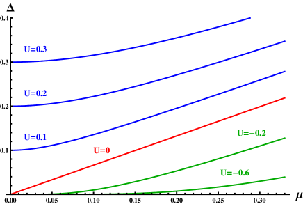
Figure 2: Order parameter at zero temperature as function of chemical potential of the TI surface Weyl semi-metal at various values of coupling parametrized by the renormalized energy $U$, Eq.(43). For positive $U$ (blue lines) the superconductivity is strong and does not vanish even for zero chemical potential. There exists the critical coupling, $U=0$ (red line), at which the second order transition occurs at quantum critical point $\mu=0$. For negative $U$ the superconductivity still exists at $\mu>0$, but is exponentially weak.

For an attractive coupling $g$ stronger than the critical one,

$$g_{c}=\frac{4\pi\hbar^{2}v_{F}}{\Lambda}\text{,}$$ (44)

(when $U>0$), blue lines in Fig. 2, there are two qualitatively different cases.

(i). When $\mu<<U$ the dependence of $\Delta$ on the chemical potential is parabolic, see Li14 . In particular, when $\mu=0,$ the gap equals $U$. As can be seen from Fig. 2, the chemical potential makes a very limited impact in the large portion of the phase diagram.

(ii) For the attraction just stronger than critical, $g>g_{c}$, namely for small positive $U$, the dependence becomes linear, see red line in Fig. 2, $\Delta=0.663\,\mu$. So that the already weak condensate becomes sensitive to $\mu$.

The case (i) is more interesting than (ii) since it exhibits stronger superconductivity (larger $T_{c}$, see below). Finally for $g<g_{c}\,$, namely negative $U$ (green lines), the superconductivity is very weak with exponential dependence similar to the BCS one, $\Delta\approx\mu$ exp$\left[-\left(\left|U\right|/\mu-1\right)\right]$. As was mentioned above, in the more interesting cases of large $\Delta$ the dependence on the chemical potential is very weak. A peculiarity of superconductivity in TI is that electrons (and holes) in Cooper pairs are created themselves by the pairing interaction rather than being present in the sample as free electrons. Therefore it is shown that it is possible to neglect the effect of weak doping and consider directly the $\mu=0$ particle-hole symmetric case. This point in parameter space is the QCP Sachdev and will be studied in detail in what follows. Of course, at finite temperature at any attraction, $g>0$, there exists a (classical) superconducting critical point at certain temperature $T_{c}$ that is calculated next.

IV.2 Dependence of the critical temperature $T_{c}$ on strength of pairing interaction.

Summation over Matsubara frequency and integrations over momenta in the gap equation, Eq.(42), at finite temperature and arbitrary chemical potential. The critical temperature as a function of $\mu$ and (positive) $U$ is obtained numerically and presented in Fig. 3. Again at relatively large $U$ the dependence of $T_{c}$ on the chemical potential is very weak and parabolic. When $0<g<g_{c}$ the critical temperature is exponentially small albeit nonzero, $\frac{\Delta}{U}\approx 1+\left(\frac{\mu}{U}\right)^{2}$.

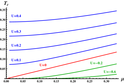
Figure 3: Transition temperature as function of chemical potential at supercritical ($U>0$, in blue), critical ($U=0$, in red) and subcritical values of coupling.

IV.3 Zero chemical potential $\mu=0$.

At zero chemical potential the Hamiltonian Eq.(1) possesses a particle - hole symmetry. Microscopically, Cooper pairs of both electrons and holes are formed, see Fig. 1a. The system is unique in this sense since the electron - hole symmetry is not spontaneously broken in both normal and superconducting phases. Supercurrent in such a system does not carry momentum or mass. Performing the sum and integral over momenta in the gap equation, Eq.(42), analytically (see Appendix A), it becomes (using the definition of $U$ given in Eq.(43)) for $U>0$:

$$U=2T\log\left[2\cosh\frac{\Delta}{2T}\right]\text{.}$$ (45)

At zero temperature $\Delta=U$, while $\Delta\rightarrow 0$ as a power of the parameter $U\propto g-g_{c}$ describing the deviation from quantum criticality

$$T_{c}=\frac{1}{2\log 2}U^{z\nu};\text{ \ }z\nu=1\text{.}$$ (46)

Here $z$ is the dynamical critical exponentSachdev . Therefore, as expected, the renormalized coupling describing the deviation from the QCP is proportional to the temperature at which the created condensate disappears.

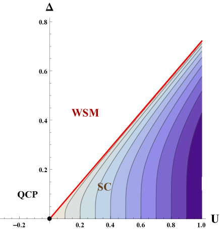
Figure 4: Phase diagram of  STI. Order parameter as function of $U$ describing the deviation from criticality near the quantum critical point at $\Delta=0$, $\mu=0$. The critical line is a strait line in mean field approximation.

The temperature dependence of the gap reads:

$$\Delta\left(T\right)=2T\cosh^{-1}\left(\frac{1}{2}\exp\frac{U}{2T}\right)\text{.}$$ (47)

This it typical for chiral universality classes Sachdev ; Rosenstein .

It is interesting to compare this dependence with the conventional BCSAGD for transition at finite temperature, namely away from QCP, see Fig 1b. At zero temperature $\Delta\left(0\right)/T_{c}=2\log 2$ $=\allowbreak 1.\,\allowbreak 39$ (within BCS - $1.76$), while near $T_{c}$ one gets $\Delta/T_{c}=2^{3/2}\log^{1/2}2\sqrt{1-t}=$ $2.\,\allowbreak 35\sqrt{1-t}$ (BCS - $3.07\sqrt{1-t}$), where $t=T/T_{c}$. To describe the behavior of the STI in inhomogeneous situations like the external magnetic field, boundaries, impurities or junction with metals or other superconductors, it is necessary to derive the effective theory in terms of the order parameter $\Delta\left(\mathbf{r}\right)$, where $\mathbf{r}$ varies on the mesoscopic scale.

Phase diagram of  STI order parameter as function of $U$ at zero temperature is plotted in Fig.4.

IV.4 Coherence length and the condensation energy

The quadratic term of the Ginzburg-Landau energy $F_{2}=\sum_{\mathbf{p}}\Delta_{p}^{\ast}\Gamma\left(p\right)\Delta_{p}$ is obtained exactly from expanding the gap equation to linear terms in $\Delta$ for arbitrary external momentum. The dependence on $\mathbf{p}$ is non-analytic and within our approximation higher powers of $p$ do not appear. The second term is very different from the quadratic term in the GL functional for conventional phase transitions at finite temperature Herbutbook or even quantum phase transitions in models without Weyl fermions Sachdev and has a number of qualitative consequences. Comparing the two terms in Eq.(51), one obtains the coherence length as a power of parameter $U\propto g-g_{c}$ describing the deviation from criticality:

$$\xi\left(U\right)=\frac{\pi}{4}v_{F}\hbar U^{-\nu}\text{; \ \ \ \ }\nu=1\text{.}$$ (48)

This is different from the dependence in non-chiral universality classes that is Herbutbook $\xi\left(T\right)\infty\left(T_{c}-T\right)^{-\nu},$ $\nu=1/2$ in mean field. Of course in the regime of critical fluctuations this exponent is corrected in both non-chiral Herbutbook and chiralGat universality classes.

Local terms in the GL energy density are also calculable exactly. Expression for the kernel can be written as a trace:

$$\Gamma=\frac{1}{2}tr\left\{\sum\limits_{\omega q}\sigma^{y}D_{\omega q}^{t}\sigma^{y}D_{\omega,q-p}+\frac{1}{g}I\right\}$$ (49)

$$=\frac{1}{g}-\sum\limits_{\omega q}\frac{\hbar^{2}\omega^{2}-v_{F}^{2}p\cdot q+v_{F}^{2}q^{2}}{\left(\hbar^{2}\omega^{2}+v_{F}^{2}q^{2}\right)\left(\hbar^{2}\omega^{2}+v_{F}^{2}\left|\mathbf{q-p}\right|^{2}\right)}.$$

Integrating over $\omega$ (at zero temperature) one obtains

$$\Gamma = -\frac{1}{8\pi^{2}\hbar^{2}v_{F}}\int_{q,\phi}\frac{pq\cos\phi-p^{2}}{\left|\mathbf{q-p}\right|^{2}+q\left|\mathbf{q-p}\right|}$$

$$-\frac{U}{4\pi\hbar^{2}v_{F}^{2}},$$

where $\phi$ is an angle between $\mathbf{q}$ and $\mathbf{p}$. The integral is homogeneous in momentum and therefore is linear in $p=\left|\mathbf{p}\right|$ and one arrives at:

$$\Gamma\left(p\right)=-\frac{U}{4\pi\hbar^{2}v_{F}^{2}}+\frac{\left|p\right|}{16v_{F}\hbar^{2}}\text{.}$$ (51)

IV.5  Local terms in Ginzburg - Landau equation and energy

For $p=0$ the gap equation Eq.(42) reads

$$\frac{\Delta}{4\pi\hbar^{2}v_{F}^{2}}\left(-U+\sqrt{\Delta^{\ast}\Delta}\right)=0\text{,}$$ (52)

This is obtained from the energy functional

$$F=\frac{1}{4\pi\hbar^{2}v_{F}^{2}}\int d^{2}\mathbf{r}\left\{-U\Delta^{\ast}\Delta+\frac{2}{3}\left(\Delta^{\ast}\Delta\right)^{3/2}\right\}\text{.}$$ (53)

It is quite nonstandard compared to customary quartic term $\left(\Delta^{\ast}\Delta\right)^{2}$ in conventional universality classes. The GL equations in the homogeneous case for the condensate gives $\Delta_{0}=U^{\beta}$ with critical exponent $\beta=1,$ different from the mean field value $\beta=1/2$ for the $U\left(1\right)$ universality classHerbutbook . The condensation energy density is $f_{0}=-\frac{1}{12\pi\hbar^{2}v_{F}^{2}}U^{2-\alpha}$ with $\alpha=-1$. The free energy critical exponent at QCP therefore is also different from the classical $\alpha=0$. The magnetic field couples to the order parameter field by a standard minimal substitution. The Ginzburg-Landau approach the only available practical tool to study properties of inhomogeneous configurationsAbrikosov in external magnetic field like the Abrikosov vortex systems.

V Exciton condensation

V.1 Chiral symmetry breaking

Assuming that the electric charge $U\left(1\right)$ and rotation symmetry is unbroken (no superconductivity) for insufficiently strong attractive interaction (pairing) one still can have transitions due to always existing effective repulsion. This possibility was already considered in grapheneGusynin . Here we note that the symmetry patten might be very different from often invoked relativistic $2+1$ Gross - Neveu model thoroughly studied as a toy model in relativistic quantum field theory. Possible chiral symmetry breaking states were reviewed in subsection IId and we consider first a ground state with nonzero order parameter

$$\left\langle P_{3}^{\left(1\right)}\right\rangle=v\not=0\text{.}$$ (54)

It is convenient to parametrize the gaussian variational ground state by the trace of propagator:

$$G\left(X;X\right)=m/g\text{ }\gamma_{0}\text{,}$$ (55)

with ”mass” $m$ determining the order parameter. According to gap equation derived in Appendix B, we have

$$G^{-1} = \left(i\omega+\mu\right)I-\alpha\cdot\left(\hbar v_{F}k\right)-m\gamma_{0};$$ (56)

$$G = -\frac{\left(\mu+i\omega\right)I+\alpha\cdot\left(\hbar v_{F}k\right)+m\gamma_{0}}{m^{2}+\left(\hbar v_{F}k\right)^{2}-\left(\mu+i\ \omega\right)^{2}\ }\text{,}$$

leads to

$$mI=gG^{\prime}\left(\tau,\mathbf{r};\tau,\mathbf{r}\right)\gamma_{0}^{-1}=-\frac{g}{\left(2\pi\right)^{3}}\times$$ (57)

$$\int_{\omega,\mathbf{k}}\frac{m}{m^{2}+\left(\hbar v_{F}\mathbf{k}\right)^{2}-\left(\mu+i\ \omega\right)^{2}\ }\text{.}$$

Performing integrations with momentum cutoff $\Lambda$ one obtains for $m\not=0$:

$$1=-\frac{g}{4\pi\left(\hbar v_{F}\right)^{2}}\left\{\begin{array}[]{c}\left(\sqrt{m^{2}+\Lambda^{2}}-m\right),\mu\leq m\\ \left(\sqrt{m^{2}+\Lambda^{2}}-\mu\right),\mu>m\end{array}\right.\text{.}$$ (58)

For $\mu=m$ one obtains the first order transition point (for $\mu>0$)

$$\text{ }\frac{4\pi\left(\hbar v_{F}\right)^{2}}{\left|g_{c}\right|}=\sqrt{\mu^{2}+\Lambda^{2}}-\mu\text{,}$$ (59)

For larger repulsion, $\left|g\right|\geqslant\left|g_{c}\right|$, the mass is larger:

$$m=\mu+\frac{1}{\left(\hbar v_{F}\right)^{2}}\left(\left|g\right|-\left|g_{c}\right|\right)\left(\frac{\Lambda^{2}}{8\pi}+\frac{2\pi\left(\hbar v_{F}\right)^{4}}{\left|g\right|\left|g_{c}\right|}\right).$$ (60)

The free energy, using the Abrikosov formula derived in Appendix B, is ($\Lambda>>m$)

$$\left(\Omega\left(m\right)-\Omega_{0}\left(m=0\right)\right)/V=\int_{0}^{m}2m^{2}\frac{d\frac{1}{\left|g\right|}}{dm}dm$$ (61)

$$=-\int_{0}^{m}\frac{m^{2}}{2\pi\left(\hbar v_{F}\right)^{2}}dm=-\frac{m^{3}}{6\pi\left(\hbar v_{F}\right)^{2}}\text{ .}$$

For $\mu>m$, since $\frac{d\left(1/\left|g\right|\right)}{dm}=\frac{1}{4\pi\left(\hbar v_{F}\right)^{2}}\frac{m}{\sqrt{m^{2}+\Lambda^{2}}}>0$, the chiral symmetry breaking state will have higher energy than the normal one. For $\left|g\right|<\left|g_{c}\right|,$ the stable ground state is the normal state with $m=0$.

Finite temperature properties including the phase diagram and the QCP at zero chemical potential can be studied along the lines similar to the superconducting transition.

VI Discussion and conclusions

Having considered both the superconducting and the excitonic transitions for sufficiently strong attraction or repulsion within the gaussian approximation, a natural question is what happens when we approach the quantum critical point. At criticality various renormalization group methods should be usedHerbutbook .

VI.1 Criticality beyond the gaussian approximation

Critical (quantum) fluctuations are expected to be significant in this relatively low dimensional (relativistic 2+1 dimensional system) system. Generally they are not as strong as in 2D statistical system at finite temperature, but stronger than in 3D one. The approximation we have made describes reasonably well ”gaussian” fluctuation beyond the region where stronger critical fluctuations in these systems appear and should be treated nonperturbativelyRosenstein typically using variants of the renormalization group approachHerbutbook . The critical exponents in this region differ from the one called ”quantum gaussian (BCS)” in ref. Sachdev and available results are obtained using either $\varepsilon$ expansionGat ; Herbut09 ($\varepsilon=4-d$, where $d=2+1$ is the space-time dimension), $1/N$, where $N$ is the number of fermionic species on the surfaceGat and functional (strong coupling) RGJanssen and Monte Carlo simulationsold ; MC (with reservations specified below). The universality class of the supconducting transition according to classification proposed in ref. Gat is the chiral XY (symmetry of order parameter $U\left(1\right)$) with $N=1$. The large $N$ expansion is not reliable for the one component system considered here (but the number might be larger in similar systems for which our approach trivially generalizes), so let us use the $\varepsilon$ expansion.

Using the formulas for the anomalous dimensions of the order parameter (see second reference in Gat ),

$$\gamma_{\Delta}=\eta=1/4\varepsilon+0.044\varepsilon^{2}+O\left(\varepsilon^{3}\right)\approx 0.294$$ (62)

and its square,

$$\gamma_{\Delta^{2}}=\left(1+\sqrt{11}\right)/10\varepsilon+0.065\varepsilon^{2}\simeq 0.43\varepsilon+0.065\varepsilon^{2},$$ (63)

critical exponents are obtained from the hyperscaling relations:

$$\alpha = 2-d/\left(2-\gamma_{\Delta^{2}}\right)=\left(\varepsilon-2\gamma_{\Delta^{2}}\right)/\left(2-\gamma_{\Delta^{2}}\right)=-0.353,$$

$$\beta = \left(1+\gamma_{\Delta}\right)/2\left(2-\gamma_{\Delta^{2}}\right)=0.515\text{.}$$ (64)

and can be compared with those in Table 1 in ref.Li14 .  The exponents from the $\varepsilon$ expansion were found to be consistent for larger values of $N$ with the latest Monte Carlo simulations MC , while consistent with the functional RGJanssen . The critical exponents of the chiral transition belongs to this class with $N=2$.

The corresponding chiral universality class for the exciton condensation in Dirac semi-metal is the Heisenberg $N=2$ ($SU\left(2\right)$). The critical exponents for this case were also calculated in ref.Gat ; Herbut09 ; Janssen Recently they were invoked in a discussion of second order quantum transitions in Hubard model on honeycomb latticeSorella . It should be noted that the flavour symmetries are often broken ”explicitly” by some kind of anisotropy. In this case Goldstone bosons acquire a small mass (like pions in quantum chromodynamics in which the chiral symmetry is slightly broken by the light quark masses), although their major properties remain intact. This can be taken into account as a small perturbationChiraldyn .

VI.2 Experimental feasibility of observation of quantum phase transition

The best candidate to observe the superconductivity is a topological insulator of the $Bi_{2}Se_{3}$ family. To estimate the pairing efficiency due to phonons, one should rely on recent studies of surface phonons in TI DasSarma . The coupling constant in the Hamiltonian, Eq.(1), is obtained from the exchange of acoustic (Rayleigh) surface phonons $g=\lambda v_{F}^{2}\hbar^{2}/2\pi\mu$, where $\lambda$ is the dimensionless effective electron - electron interaction constant of order $0.1$ (somewhat lower values are obtained in ref.Guinea ). It was shown in ref. DasSarma that at zero temperature the ratio of $\lambda$ and $\mu$ is constant with well defined $\mu\rightarrow 0$ limit with value $g=0.23$ $eV\ nm^{2}$ for $v_{F}\approx 7\ \cdot 10^{5}m/s$ (for $Bi_{2}Se_{3}$). The critical coupling constant $g_{c}$, Eq.(44), can be estimated from the Debye cutoff $T_{D}=200K$ determining the momentum cutoff $\Lambda=T_{D}/c_{s}$, where $c_{s}$ is the sound velocity. Taking value to be $c_{s}=2\cdot 10^{3}m/s$ (for $Bi_{2}Se_{3}$), one obtains $g_{c}=4\pi v_{F}c_{s}\hbar^{2}/\,T_{D}=0.20$ $eV$ $nm^{2}$.

Of course the Coulomb repulsion might weaken or even overpower the effect of the attraction due to phonons, so that superconductivity does not occur. In TI like $Bi_{2}Se_{3}$ however, the dielectric constant is very large $\varepsilon=50$, so that the Coulomb repulsion is weak. Moreover it was found in graphene (that has identical Coulomb interaction), that although the semi-metal does not screen CastroNeto , the effects of the Coulomb coupling are surprisingly small, even in leading order in perturbation theory. The superconductivity was observed in these systems that howeved had to be either doped in the bulk or on the surfaceKoren (by a $Cu$) or by applying pressurepressureBiSe . It is not yet clear whether the observed superconductivity is a bulk or a surface effect.

The Dirac semimetal in optically trapped cold atomscold offers a well controllable system in which this phenomenon occurs both for repulsive interaction (chiral symmetry breaking) and in particular the attractive one (superconductivity) becuase there is no Coulomb repulsion as the atoms are neutral.

Recently after experimental discovery of 3D Dirac semi-metalsPotemski the new class of questions similar to those discussed in present paper arise. Extraordinary electronic properties of these Dirac materials3Dtheory including superconductivityCava and chiral condensate are being studied theoretically and experimentally.

VI.3 Conclusions

We have studied continuous phase transitions in a Dirac semi-metal realized recently as a surface of topological insulator. The noninteracting system is characterized by (nearly) zero density of states on the 2D Fermi manifold. It degenerates into a point when the chemical potential coincides with the Weyl point of the surface states as in the original proposal for a major class of such materialsZhang1 . The pairing attraction (the most plausible candidate being surface phonons) therefore has two tasks in order to create the superconducting condensate. The first is to create a pair of electrons (that in the present circumstances means creating two holes as well) and the second is to pair them. To create the charges does not cost much energy since the spectrum of the Weyl semimetal is gapless (massless relativistic fermions); this is effective as long as the coupling $g$ is larger than the critical $g_{c}$, see Eq.(44). The situation is more reminiscent of the creation of the chiral condensate in relativistic massless four - fermion theory (a 2D versionRosenstein was recently contemplated for graphene CastroNeto ; Katsnelson ) than to the BCS or even BEC in condensed matter systems with parabolic dispersion law. Due to the special ”ultra-relativistic” nature of the pairing transition at zero temperature as a function of parameters like the pairing interaction strength is unusual: even the mean field critical exponents are different from the standard ones that generally belong to the $U\left(1\right)$ class of second order phase transitions.

To summarize, we studied the phase diagram of the superconducting and chiral transition at arbitrary chemical potential, effective local interaction strength and temperature $T$. The quantum ($T=0$) critical point appears at zero chemical potential and belongs the $U_{N}\left(1\right)$ chiral universality class (the subscript denotes number of massless fermions at QCP according to classification in Gat ; Sachdev ) for the attraction (superconductivity) and $SU_{N}\left(2\right)$ for repulsion (exciton condensation).

Acknowledgements. We are indebted to C.W. Luo, J.J. Lin and W.B. Jian for explaining details of experiments, and T. Maniv and M. Lewkowicz for valuable discussions. Work of D.L. and B.R. was supported by NSC of R.O.C. Grants No. 98-2112-M-009-014-MY3 and MOE ATU program. The work of D.L. also is supported by National Natural Science Foundation of China (No. 11274018). B.R. is grateful to School of Physics of Peking University for hospitslity.

Appendix A Path integral derivation of the Gorkov and Dyson - Schwinger equations

A.1 General correlations and sources

We introduce the grassmanian source terms into Matsubara action Eq.(3):

$$S\left[\psi^{+}\mathbf{,}\psi,J^{+},J\right]=S\left[\psi^{+}\mathbf{,}\psi\right]$$ (65)

$$-\int_{0}^{\beta}d\tau\int_{r}\left[\psi_{\sigma}^{+}\left(\tau,\mathbf{r}\right)J_{\sigma}\left(\tau,\mathbf{r}\right)+\psi_{\sigma}\left(\tau,\mathbf{r}\right)J_{\sigma}^{+}\left(\tau,\mathbf{r}\right)\right]\text{.}$$

The generating functional for the disconnected correlations is $Z\left(J^{+},J\right)$

$$\left\langle\psi_{\alpha}\left(X\right)\right\rangle = \frac{1}{Z}\frac{\delta Z}{\left[-\delta J_{\alpha}^{+}\left(X\right)\right]}\text{;}$$ (66)

$$\left\langle T\psi_{\alpha}\left(X\right)\psi_{\beta}\left(X^{\prime}\right)...\right\rangle_{u} = \frac{1}{Z}\frac{\delta Z}{\left[-\delta J_{\alpha}^{+}\left(X\right)\right]\left[-\delta J_{\beta}^{+}\left(X^{\prime}\right)\right]...}\text{,}$$

where $X=\left(\mathbf{r,}\tau\right)$, $X^{\prime}=\left(\mathbf{r}^{\prime},\tau^{\prime}\right)$. The correlators is (Matsubara) time ordered. The generating functional for the connected correlations are $W=-\ln Z\left(J^{+},J\right)$:

$$\left\langle\psi_{\alpha}\left(X\right)\right\rangle = \frac{\delta W}{\delta J_{\alpha}^{+}\left(X\right)}\text{,}$$ (67)

$$\left\langle T\psi_{\alpha}\left(X\right)\psi_{\beta}\left(X^{\prime}\right)...\right\rangle = -\frac{\delta W}{\left[-\delta J_{\alpha}^{+}\left(X\right)\right]\left[-\delta J_{\beta}^{+}\left(X^{\prime}\right)\right]...}\text{.}$$

In particular, we define the normal and anomalous Green’s functions (see ref.AGD ) as,

$$\left\langle T\psi_{\alpha}\left(X\right)\psi_{\beta}^{+}\left(X^{\prime}\right)\right\rangle = -\frac{\delta W}{\delta J_{\alpha}\left(X\right)\delta J_{\beta}^{+}\left(X^{\prime}\right)}=-G_{\alpha\beta}\left(X\mathbf{;}X^{\prime}\right)\text{;}$$

$$\left\langle T\psi_{\alpha}\left(X\right)\psi_{\beta}\left(X^{\prime}\right)\right\rangle = -\frac{\delta W}{\delta J_{\alpha}^{+}\left(X\right)\delta J_{\beta}^{+}\left(X^{\prime}\right)}=F_{\alpha\beta}\left(X\mathbf{;}X^{\prime}\right)\text{;}$$

$$\left\langle T\psi_{\alpha}^{+}\left(X\right)\psi_{\beta}^{+}\left(X^{\prime}\right)\right\rangle = -\frac{\delta W}{\delta J_{\alpha}\left(X\right)\delta J_{\beta}\left(X^{\prime}\right)}=F_{\alpha\beta}^{+}\left(X\mathbf{;}X^{\prime}\right)$$ (68)

where we denote $\left\langle\psi_{\alpha}\left(X\right)\right\rangle$ as $\psi_{\alpha}\left(X\right)$, and drop the time ordering operation $T$ in correlators. For example, $\left\langle\psi_{\alpha}\left(X\right)\psi_{\beta}\left(X^{\prime}\right)\right\rangle$ stands for $\left\langle T\psi_{\alpha}\left(X\right)\psi_{\beta}\left(X^{\prime}\right)\right\rangle$.

A.2 Derivation of the Gor’kov equation for superconductivity

Using identities,

$$\int D\psi^{+}D\psi\frac{\delta}{\delta\psi_{\alpha}^{+}\left(X\right)}e^{-\frac{1}{\hbar}S\left[\psi^{+}\mathbf{,}\psi,J^{+},J\right]} = 0\text{;}$$ (69)

$$\int D\psi^{+}D\psi\frac{\delta}{\delta\psi_{\alpha}\left(X\right)}e^{-\frac{1}{\hbar}S\left[\psi^{+}\mathbf{,}\psi,J^{+},J\right]} = 0\text{,}$$

the equations of motions lead to

$$\left(\hbar\partial_{\tau}\delta_{\alpha\beta}+K_{\alpha\beta}\left(\mathbf{\nabla}\right)\right)\psi_{\beta}\left(X\right)\mathbf{-}g\times$$

$$\left\langle\psi_{\beta}^{+}\left(X\right)\psi_{\beta}\left(X\right)\psi_{\alpha}\left(X\right)\right\rangle=J_{\alpha}\left(\tau,\mathbf{r}\right)\text{,}$$ (70)

$$\left(\hbar\partial_{\tau}\delta_{\alpha\beta}-\widehat{K}_{\beta\alpha}\left(-\mathbf{\nabla}\right)\right)\psi_{\beta}^{+}\left(X\right)\mathbf{+}g\times$$

$$\left\langle\psi_{\alpha}^{+}\left(X\right)\psi_{\beta}^{+}\left(X\right)\psi_{\beta}\left(X\right)\right\rangle=J_{\alpha}^{+}\left(\tau,\mathbf{r}\right)\text{. }$$

Generally full correlations of the fields can be expressed via connected correlators. For example,

$$\left\langle\psi_{\beta}^{+}\left(X\right)\psi_{\beta}\left(X\right)\psi_{\alpha}\left(X\right)\right\rangle=\psi_{\beta}^{+}\left(X\right)\psi_{\beta}\left(X\right)\psi_{\alpha}\left(X\right)-$$

$$\psi_{\alpha}\left(X\right)\left\langle\psi_{\beta}\left(X\right)\psi_{\beta}^{+}\left(X\right)\right\rangle_{c}+\psi_{\beta}\left(X\right)\times$$ (71)

$$\left\langle\psi_{\alpha}\left(X\right)\psi_{\beta}^{+}\left(X\right)\right\rangle_{c}+\left\langle\psi_{\beta}^{+}\left(X\right)\right\rangle\left\langle\psi_{\beta}\left(X\right)\psi_{\alpha}\left(X\right)\right\rangle$$

$$+\left\langle\psi_{\beta}^{+}\left(X\right)\psi_{\beta}\left(X\right)\psi_{\alpha}\left(X\right)\right\rangle_{c}\text{.}$$

For Gaussian mean field approximation, we omit higher order connected correlations, like $\left\langle\psi_{\beta}^{+}\left(X\right)\psi_{\beta}\left(X\right)\psi_{\alpha}\left(X\right)\right\rangle$,

$$J_{\alpha}\left(X\right)=\left(\hbar\partial_{\tau}\delta_{\alpha\beta}+K_{\alpha\beta}\right)\psi_{\beta}\left(X\right)\mathbf{-}g\times$$ (72)

$$\psi_{\beta}^{+}\left(X\right)\psi_{\beta}\left(X\right)\psi_{\alpha}\left(X\right)-\psi_{\alpha}\left(X\right)\left\langle\psi_{\beta}\left(X\right)\psi_{\beta}^{+}\left(X\right)\right\rangle_{c}$$

$$+\psi_{\beta}\left(X\right)\left\langle\psi_{\alpha}\left(X\right)\psi_{\beta}^{+}\left(X\right)\right\rangle_{c}+\psi_{\beta}^{+}\left(X\right)\left\langle\psi_{\beta}\left(X\right)\psi_{\alpha}\left(X\right)\right\rangle_{c}$$

Performing functional derivative$\frac{\delta}{\delta J_{\gamma}\left(X^{\prime}\right)}$ (by using the identity, $\frac{\delta}{\delta J_{\gamma}\left(X^{\prime}\right)}\psi_{\alpha}\left(X\right)=\left\langle\psi_{\alpha}\left(X\right)\psi_{\gamma}^{+}\left(X^{\prime}\right)\right\rangle$, the correlators of odd number of Grassmannians vanishing) and taking at the end $J_{\alpha}\left(X\right)=0$, one obtains:

$$\delta\left(X\mathbf{-}X^{\prime}\right)\delta_{\alpha\gamma}=\left(\partial_{\tau}\delta_{\alpha\beta}+\widehat{K}_{\alpha\beta}\right)\left\langle\psi_{\beta}\left(X\right)\psi_{\gamma}^{+}\left(X^{\prime}\right)\right\rangle\mathbf{-}g$$

$$\times\left\{-\left\langle\psi_{\alpha}\left(X\right)\psi_{\gamma}^{+}\left(X^{\prime}\right)\right\rangle\left\langle\psi_{\beta}\left(X\right)\psi_{\beta}^{+}\left(X\right)\right\rangle\right.$$ (73)

$$+\left\langle\psi_{\beta}\left(X\right)\psi_{\gamma}^{+}\left(X^{\prime}\right)\right\rangle\left\langle\psi_{\alpha}\left(X\right)\psi_{\beta}^{+}\left(X\right)\right\rangle$$

$$+\left.\left\langle\psi_{\beta}^{+}\left(X\right)\psi_{\gamma}^{+}\left(X^{\prime}\right)\right\rangle\left\langle\psi_{\beta}\left(X\right)\psi_{\alpha}\left(X\right)\right\rangle\right\}\text{,}$$

or

$$\delta\left(X-X^{\prime}\right)\delta_{\alpha\gamma}=\left(-\partial_{\tau}\delta_{\alpha\beta}-\widehat{K}_{\alpha\beta}\right)G_{\beta\gamma}\left(X,X^{\prime}\right)\mathbf{-}g$$

$$\times\left\{-G_{{}_{\alpha}\gamma}\left(X,X^{\prime}\right)G_{\beta\beta}\left(X,X\right)\right.$$ (74)

$$+G_{\beta\gamma}\left(X,X^{\prime}\right)G_{\alpha\beta}\left(X,X\right)_{c}+$$

$$\left.F_{\beta\gamma}^{+}\left(X,X^{\prime}\right)F_{\beta\alpha}\left(X,X\right)\right\}\text{.}$$

Similarly the second equation of motion,

$$J_{\alpha}^{+}\left(\tau,\mathbf{r}\right)=\left(\partial_{\tau}\delta_{\alpha\beta}-\widehat{K}_{\beta\alpha}\left(-\mathbf{\nabla}\right)\right)\left\langle\psi_{\beta}^{+}\left(\tau,\mathbf{r}\right)\right\rangle\mathbf{+}g$$

$$\left\{\left\langle\psi_{\alpha}^{+}\left(\tau,\mathbf{r}\right)\psi_{\beta}^{+}\left(\tau,\mathbf{r}\right)\right\rangle\left\langle\psi_{\beta}\left(\tau,\mathbf{r}\right)\right\rangle\right.$$ (75)

$$-\left\langle\psi_{\alpha}^{+}\left(\tau,\mathbf{r}\right)\right\rangle\left\langle\psi_{\beta}\left(\tau,\mathbf{r}\right)\psi_{\beta}^{+}\left(\tau,\mathbf{r}\right)\right\rangle$$

$$+\left.\left\langle\psi_{\beta}^{+}\left(\tau,\mathbf{r}\right)\right\rangle\left\langle\psi_{\beta}\left(\tau,\mathbf{r}\right)\psi_{\alpha}^{+}\left(\tau,\mathbf{r}\right)\right\rangle\right\}\text{,}$$

gives

$$\left(\partial_{\tau}\delta_{\alpha\beta}-\widehat{K}_{\beta\alpha}\left(-\mathbf{\nabla}\right)\right)F_{\beta\gamma}^{+}\left(X,X^{\prime}\right)+g\left\{-F_{\alpha\beta}^{+}\left(X,X\right)\right.$$

$$G_{\beta\gamma}\left(X,X^{\prime}\right)+F_{\alpha\gamma}^{+}\left(X,X^{\prime}\right)G_{\beta\beta}\left(X,X\right)+$$ (76)

$$\left.G_{\beta\alpha}\left(X,X\right)F_{\beta\gamma}^{+}\left(X,X^{\prime}\right)\right\}=0\text{.}$$

In the superconducting phase, if the spin rotation invariance is not broken and chiral symmetry is preserved, $G_{\alpha\beta}\left(X,X\right)=G_{\alpha\beta}^{c}=n_{c}\delta_{\alpha\beta}$. For the $N$ component spinors $n_{c}=n/N$, where $n$ is the density of electrons. The quadratic parts of Eqs.(74,76) simplify:

$$\mathbf{-}g\left\{-G_{\alpha\gamma}\left(X,X^{\prime}\right)G_{\beta\beta}\left(X,X\right)+G_{\beta\gamma}\left(X,X^{\prime}\right)G_{\alpha\beta}\left(X,X\right)\right\}$$

$$=\mathbf{-}g\left\{-G_{\alpha\gamma}\left(X,X^{\prime}\right)Nn_{c}+n_{c}G_{\alpha\gamma}\left(X,X^{\prime}\right)\right\}$$

$$=g\left(N-1\right)n_{c}G_{\alpha\gamma}\left(X,X^{\prime}\right);$$ (77)

$$g\left\{F_{\alpha\gamma}^{+}\left(X,X^{\prime}\right)G_{\beta\beta}\left(X,X\right)+G_{\beta\alpha}\left(X,X\right)F_{\beta\gamma}^{+}\left(X,X^{\prime}\right)\right\}$$

$$=-g\left(N-1\right)n_{c}F_{\alpha\gamma}^{+}\left(X,X^{\prime}\right)\text{,}$$

and such terms can be absorbed to the chemical potential term with the chemical potential replaced by the renormalized

$$\mu+g\left(N-1\right)n_{c}=\mu_{R}\text{.}$$ (78)

Therefore we finally obtain the Gor’kov equations, given in Eqs.(12).

A.3 Derivation of DS equation and renormalized chemical potential for nonsuperconducting state.

We need only to discuss the equation for $\frac{\delta J_{\alpha}}{\delta\psi_{\beta}}$, as$\frac{\delta J_{\alpha}^{+}}{\delta\psi_{\beta}^{+}}$ is just the complex conjugate of $\frac{\delta J_{\alpha}}{\delta\psi_{\beta}}$ and $\frac{\delta J_{\alpha}^{+}}{\delta\psi_{\beta}}=\frac{\delta J_{\alpha}}{\delta\psi_{\beta}^{+}}=0$. We reorganize the equation $\frac{\delta J_{\alpha}}{\delta\psi_{\beta}}$as

$$\frac{\delta J_{\alpha}}{\delta\psi_{\beta}}=\left(\partial_{\tau}\delta_{\alpha\beta}+K_{\alpha\beta}\right)\delta\left(X-X^{\prime}\right)-g\delta\left(X-X^{\prime}\right)\times$$

$$\left\{\left\langle\psi_{\alpha}\left(X\right)\psi_{\beta}^{+}\left(X\right)\right\rangle_{c}-\frac{1}{4}\delta_{\alpha\beta}\sum\left\langle\psi_{\gamma}\left(X\right)\psi_{\gamma}^{+}\left(X\right)\right\rangle_{c}\right\}$$

$$+g\delta_{\alpha\beta}\delta\left(X-X^{\prime}\right)\left\{\left\langle\psi_{\beta}\left(X\right)\psi_{\beta}^{+}\left(X\right)\right\rangle_{c}-\right.$$ (79)

$$\left.\sum\left\langle\psi_{\gamma}\left(X\right)\psi_{\gamma}^{+}\left(X\right)\right\rangle_{c}\right\}\text{,}$$

The last two terms are proportional to $\delta_{\alpha\beta}$, and can be absorbed to the chemical potential,

$$\mu+g\delta_{\alpha\beta}\left\{\sum\left\langle\psi_{\gamma}\left(X\right)\psi_{\gamma}^{+}\left(X\right)\right\rangle_{c}\right.$$ (80)

$$-\left.\left\langle\psi_{\beta}\left(X\right)\psi_{\beta}^{+}\left(X\right)\right\rangle_{c}\right\}=\mu_{R\text{.}}$$

The gap equation can be recasted as

$$G^{-1} = G_{0}^{-1}+g\delta\left(X-X^{\prime}\right)G^{\prime}\left(X;X^{\prime}\right)$$

$$G_{0}^{-1} = \left(\partial_{\tau}\delta_{\alpha\beta}+K_{\alpha\beta}\right)\delta\left(X-X^{\prime}\right)$$ (81)

$$G_{\alpha\beta}^{\prime}\left(X;X^{\prime}\right) = -\left\{\left\langle\psi_{\alpha}\left(X\right)\psi_{\beta}^{+}\left(X^{\prime}\right)\right\rangle_{c}-\right.$$

$$\left.\frac{1}{4}\delta_{\alpha\beta}\sum\left\langle\psi_{\gamma}\left(X\right)\psi_{\gamma}^{+}\left(X^{\prime}\right)\right\rangle_{c}\right\},$$

where $G_{\alpha\beta}^{\prime}$ is the traceless part of $G_{\alpha\beta}$, and the chemical potential in $K_{\alpha\beta}$ is $\mu_{R\text{.}}$

Appendix B A formula for energy of the superconducting state

B.1 Gap equation in the Nambu notation

A compact representation of the Gorkov equations for superconductors is the Nambu notations

$$\mathcal{G}_{\alpha\beta}\left(X,X^{\prime}\right) = \begin{pmatrix}\frac{\delta\psi_{\alpha}\left(X\right)}{\delta J_{\beta}\left(X^{\prime}\right)}&\frac{\delta\psi_{\alpha}\left(X\right)}{\delta J_{\beta}^{+}\left(X^{\prime}\right)}\\ \frac{\delta\psi_{\alpha}^{+}\left(X\right)}{\delta J_{\beta}\left(X^{\prime}\right)}&\frac{\delta\psi_{\alpha}^{+}\left(X\right)}{\delta J_{\beta}^{+}\left(X^{\prime}\right)}\end{pmatrix}$$

$$= \begin{pmatrix}-G_{\alpha\beta}\left(x,\tau;x^{\prime},\tau^{\prime}\right)&F_{\alpha\beta}\left(x,\tau;x^{\prime},\tau^{\prime}\right)\\ F_{\alpha\beta}^{+}\left(x,\tau;x^{\prime},\tau^{\prime}\right)&G_{\beta\alpha}\left(x^{\prime},\tau^{\prime};x,\tau\right)\end{pmatrix}$$

so that

$$\begin{pmatrix}\frac{\delta J_{\alpha}}{\delta\psi_{\beta}}&\frac{\delta J_{\alpha}}{\delta\psi_{\beta}^{+}}\\ \frac{\delta J_{\alpha}^{+}}{\delta\psi_{\beta}}&\frac{\delta J_{\alpha}^{+}}{\delta\psi_{\beta}^{+}}\end{pmatrix}=\mathcal{G}_{\alpha\beta}^{-1}\text{.}$$ (83)

.The functional identity

$$\frac{\delta J_{\alpha}\left(X\right)}{\delta\psi_{\beta}}\frac{\delta\psi_{\beta}}{\delta J_{\gamma}\left(X^{\prime}\right)}+\frac{\delta J_{\alpha}\left(X\right)}{\delta\psi_{\beta}^{+}}\times$$ (84)

$$\frac{\delta\psi_{\beta}^{+}}{\delta J_{\gamma}\left(X^{\prime}\right)}=\delta_{\alpha\gamma}\left(X-X^{\prime}\right)\text{,}$$

where abbreviations

$$\frac{\delta J_{\alpha}\left(X\right)}{\delta\psi_{\beta}}\frac{\delta\psi_{\beta}}{\delta J_{\gamma}\left(X^{\prime}\right)}\equiv\sum_{\beta}\int dX^{\prime\prime}\frac{\delta J_{\alpha}\left(X\right)}{\delta\psi_{\beta}\left(X^{\prime\prime}\right)}\times$$ (85)

$$\frac{\delta\psi_{\beta}\left(X^{\prime\prime}\right)}{\delta J_{\gamma}\left(X^{\prime}\right)}\text{, \ \ }\delta_{\alpha\gamma}\left(X-X^{\prime}\right)=\delta_{\alpha\gamma}\delta\left(X-X^{\prime}\right),$$

are used. In the Nambu matrix form it reads

$$\begin{pmatrix}\frac{\delta J_{\alpha}}{\delta\psi_{\beta}}&\frac{\delta J_{\alpha}}{\delta\psi_{\beta}^{+}}\\ \frac{\delta J_{\alpha}^{+}}{\delta\psi_{\beta}}&\frac{\delta J_{\alpha}^{+}}{\delta\psi_{\beta}^{+}}\end{pmatrix}\begin{pmatrix}\frac{\delta\psi_{\beta}}{\delta J_{\gamma}}&\frac{\delta\psi_{\beta}}{\delta J_{\gamma}^{+}}\\ \frac{\delta\psi_{\beta}^{+}}{\delta J_{\gamma}}&\frac{\delta\psi_{\beta}^{+}}{\delta J_{\gamma}^{+}}\end{pmatrix}=\begin{pmatrix}\delta_{\alpha\gamma}&0\\ 0&\delta_{\alpha\gamma}\end{pmatrix}\text{.}$$ (86)

The derivatives are:

$$\frac{\delta J_{\alpha}\left(X\right)}{\delta\psi_{\beta}\left(X^{\prime}\right)} = \left(\partial_{\tau}\delta_{\alpha\beta}+K_{\alpha\beta}\right)\delta\left(X-X^{\prime}\right);$$

$$\frac{\delta J_{\alpha}\left(X\right)}{\delta\psi_{\beta}^{+}\left(X^{\prime}\right)} = g\delta\left(X-X^{\prime}\right)\left\langle\psi_{\alpha}\left(\tau,\mathbf{r}\right)\psi_{\beta}\left(\tau,\mathbf{r}\right)\right\rangle_{c};$$

$$\frac{\delta J_{\alpha}^{+}\left(X\right)}{\delta\psi_{\beta}\left(X^{\prime}\right)} = g\delta\left(X-X^{\prime}\right)\left\langle\psi_{\alpha}^{+}\left(\tau,\mathbf{r}\right)\psi_{\beta}^{+}\left(\tau,\mathbf{r}\right)\right\rangle;$$ (87)

$$\frac{\delta J_{\alpha}^{+}\left(X\right)}{\delta\psi_{\beta}^{+}\left(X^{\prime}\right)} = \left(\partial_{\tau}\delta_{\alpha\beta}-K_{\beta\alpha}\left(-\mathbf{\nabla}\right)\right)\delta\left(X-X^{\prime}\right).$$

For the non-interacting model

$$\mathcal{G}_{0}^{-1} = \begin{pmatrix}\left(\mathcal{G}_{0}^{-1}\right)_{11}&0\\ 0&\left(\mathcal{G}_{0}^{-1}\right)_{22}\end{pmatrix}\text{,}$$

$$\left(\mathcal{G}_{0}^{-1}\right)_{11} = \left(\partial_{\tau}\delta_{\alpha\beta}+K_{\alpha\beta}\left(\mathbf{\nabla}\right)\right)\delta\left(x-x^{\prime},\tau-\tau^{\prime}\right);$$ (88)

$$\left(\mathcal{G}_{0}^{-1}\right)_{22} = \left(\partial_{\tau}\delta_{\alpha\beta}-K_{\beta\alpha}\left(-\mathbf{\nabla}\right)\right)\delta\left(x-x^{\prime},\tau-\tau^{\prime}\right),$$

and the gap equation can be cast in the Dyson form

$$\mathcal{G}^{-1} = \mathcal{G}_{0}^{-1}+\begin{pmatrix}0&\Sigma_{12}\\ \Sigma_{21}&0\end{pmatrix}\text{;}$$

$$\Sigma_{12} = g\delta\left(x-x^{\prime},\tau-\tau^{\prime}\right)\left\langle\psi_{\alpha}\left(\tau,\mathbf{r}\right)\psi_{\beta}\left(\tau,\mathbf{r}\right)\right\rangle_{c}\text{;}$$ (89)

$$\Sigma_{21} = g\delta\left(x-x^{\prime},\tau-\tau^{\prime}\right)\left\langle\psi_{\alpha}^{+}\left(\tau,\mathbf{r}\right)\psi_{\beta}^{+}\left(\tau,\mathbf{r}\right)\right\rangle.$$

B.2 Derivation of the expression for energy density

The free energy is

$$\Omega[\mathcal{G}]=-\frac{1}{\beta}\left\{{\frac{1}{2}}\text{Tr}\{-\ln\mathcal{G}+[\mathcal{G}_{0}^{-1}\mathcal{G}-1]\}+\Phi[\mathcal{G}]\ \right\}\text{,}$$ (90)

where in Gaussian approximation,

$$\Phi[\mathcal{G}]=\frac{g}{2}\int_{\tau,r}F_{\alpha\beta}\left(X;X\right)F_{\beta\alpha}^{+}\left(X;X\right).$$ (91)

The gap equation can be also obtained by $\frac{\delta}{\delta\mathcal{G}}\Omega[\mathcal{G}]=0$.

The energy difference between the superconducting state and normal state can be obtained by the differentiating of the grand canonical potential with respect to the coupling constant:$\frac{d}{dg}\Omega[\mathcal{G}]$. The green function $\mathcal{G}$ is dependent on $g$, but due to $\frac{\delta}{\delta\mathcal{G}}\Omega\left[\mathcal{G},g\right]=0$,

$$\frac{d}{dg}\Omega\left[\mathcal{G},g\right] = \frac{\partial}{\partial g}\Omega\left[\mathcal{G},g\right]$$

$$= -\frac{1}{2\beta}\int_{\tau,r}F_{\alpha\beta}\left(X;X\right)F_{\beta\alpha}^{+}\left(X;X\right)\text{.}$$

For homogeneous state, $F_{\alpha\beta}\left(X;X\right),F_{\beta\alpha}^{+}\left(X;X\right)$ are constant  (not dependent on $x,\tau$), and we introduce

$$F_{\alpha\beta}\left(X;X\right) = \frac{1}{g}\Delta_{\alpha\beta},F_{\alpha\beta}^{+}\left(X;X\right)$$

$$= \frac{1}{g}\Delta_{\alpha\beta}^{+}=\frac{1}{g}\Delta_{\beta\alpha}^{\ast}\text{,}$$

we obtain the free energy formula Abrikosov

$$\frac{d}{dg}\Omega[\mathcal{G]}\mathcal{=-} \frac{V}{2}\frac{1}{g^{2}}\text{Tr}\left(\Delta\Delta^{+}\right)\rightarrow$$ (94)

$$d\Omega[\mathcal{G]} \mathcal{=} \frac{V}{2}d\left(\frac{1}{g}\right)\text{Tr}\left(\Delta\Delta^{+}\right).$$

Appendix C Gap equation and free energy for chiral symmetry breaking states

C.1 Derivation of the gap equation

We will discuss the non-superconducting state with $G_{\alpha\beta}\left(X,X\right)\neq n_{c}\delta_{\alpha\beta}$, $F_{\alpha\beta}\left(X;X^{\prime}\right)=0$, which happens for example in the case of chiral symmetry breaking (CSB) state. We need only to discuss the equation for $\frac{\delta J_{\alpha}}{\delta\psi_{\beta}}$, as$\frac{\delta J_{\alpha}^{+}}{\delta\psi_{\beta}^{+}}$ is just the complex conjugate of $\frac{\delta J_{\alpha}}{\delta\psi_{\beta}}$ and $\frac{\delta J_{\alpha}^{+}}{\delta\psi_{\beta}}=\frac{\delta J_{\alpha}}{\delta\psi_{\beta}^{+}}=0$. We reorganize the equation $\frac{\delta J_{\alpha}}{\delta\psi_{\beta}}$as

$$\frac{\delta J_{\alpha}}{\delta\psi_{\beta}}=\left(\partial_{\tau}\delta_{\alpha\beta}+\widehat{K}_{\alpha\beta}\right)\delta\left(X-X^{\prime}\right)-g\delta\left(X-X^{\prime}\right)\times$$

$$\left\{\left\langle\psi_{\alpha}\left(X\right)\psi_{\beta}^{+}\left(X\right)\right\rangle_{c}-\frac{1}{4}\delta_{\alpha\beta}\right.\times$$ (95)

$$\left.\sum\left\langle\psi_{\gamma}\left(X\right)\psi_{\gamma}^{+}\left(X\right)\right\rangle_{c}\right\}+g\delta_{\alpha\beta}\delta\left(X-X^{\prime}\right)\times$$

$$\left\{\left\langle\psi_{\beta}\left(X\right)\psi_{\beta}^{+}\left(X\right)\right\rangle_{c}-\sum\left\langle\psi_{\gamma}\left(X\right)\psi_{\gamma}^{+}\left(X\right)\right\rangle_{c}\right\}\text{,}$$

The last two terms are proportional to $\delta_{\alpha\beta}$, and can be absorbed to the chemical potential,

$$\mu+g\delta_{\alpha\beta}\left\{\sum\left\langle\psi_{\gamma}\left(X\right)\psi_{\gamma}^{+}\left(X\right)\right\rangle_{c}-\right.$$ (96)

$$\left.\left\langle\psi_{\beta}\left(X\right)\psi_{\beta}^{+}\left(X\right)\right\rangle_{c}\right\}=\mu_{R\text{.}}$$

The gap equation can be recasted as

$$G^{-1} = G_{0}^{-1}+g\delta\left(X-X^{\prime}\right)G^{\prime}\left(X;X^{\prime}\right)$$

$$G_{0}^{-1} = \left(\partial_{\tau}\delta_{\alpha\beta}+\widehat{K}_{\alpha\beta}\right)\delta\delta\left(X-X^{\prime}\right)$$

$$G_{\alpha\beta}^{\prime}\left(X;X^{\prime}\right) = -\left\{\left\langle\psi_{\alpha}\left(X\right)\psi_{\beta}^{+}\left(X^{\prime}\right)\right\rangle_{c}-\right.$$

$$\left.\frac{1}{4}\delta_{\alpha\beta}\sum\left\langle\psi_{\gamma}\left(X\right)\psi_{\gamma}^{+}\left(X^{\prime}\right)\right\rangle_{c}\right\},$$

where $G_{\alpha\beta}^{\prime}$ is the traceless part of $G_{\alpha\beta}$, and the chemical potential in $\widehat{K}_{\alpha\beta}$ is $\mu_{R\text{.}}$The free energy is now

$$\Omega[\mathcal{G}] = -\left(\beta\right)^{-1}\left\{\text{Tr}\{-\ln G+[G_{0}^{-1}G-1]\}\right.$$

$$\left.+\Phi[G]\right\}\text{,}$$

where

$$\Phi[\mathcal{G}]=-\frac{g}{2}\int_{\tau,r}G_{\alpha\beta}^{\prime}\left(x,\tau;x,\tau\right)G_{\beta\alpha}^{\prime}\left(x,\tau;x,\tau\right)\text{.}$$ (99)

A similar free energy equation can be obtained,

$$\frac{d}{dg}\Omega\left[\mathcal{G},g\right] = \frac{\partial}{\partial g}\Omega\left[\mathcal{G},g\right]$$

$$= \frac{1}{2\beta}\int_{\tau,r}G_{\alpha\beta}^{\prime}\left(x,\tau;x,\tau\right)G_{\beta\alpha}^{\prime}\left(x,\tau;x,\tau\right).$$

C.2 Details of the calculation of the condensate and energy

Using the integral

$$\int_{\omega}\frac{1}{m^{2}+\left(\hbar v_{F}k\right)^{2}-\left(\mu+i\ \omega\right)^{2}\ }=$$ (101)

$$\frac{\pi}{\sqrt{m^{2}+\left(\hbar v_{F}k\right)^{2}}}\Theta\left(\sqrt{m^{2}+\left(\hbar v_{F}k\right)^{2}}-\mu\right),$$

and

$$\frac{1}{\left(2\pi\right)^{3}}\int_{\omega,p}\frac{1}{m^{2}+p^{2}-\left(\mu+i\ \omega\right)^{2}\ }$$

$$=\frac{1}{4\pi}\int_{p=0}^{\Lambda}\frac{p\Theta\left(\sqrt{m^{2}+p^{2}}-\mu\right)}{\sqrt{m^{2}+p^{2}}}$$ (102)

$$=\left\{\begin{array}[]{c}\frac{1}{4\pi}\left(\sqrt{m^{2}+\Lambda^{2}}-m\right),\mu\leq m\\ \frac{1}{4\pi}\left(\sqrt{m^{2}+\Lambda^{2}}-\mu\right),\mu>m\end{array}\right.$$ (105)

the gap equation becomes:

$$m=-\frac{g}{4\pi\left(\hbar v_{F}\right)^{2}}\left\{\begin{array}[]{c}\left(\sqrt{m^{2}+\Lambda^{2}}-m\right),\mu\leq m\\ \left(\sqrt{m^{2}+\Lambda^{2}}-\mu\right),\mu>m\end{array}\right.\text{.}$$ (106)

Appendix D Symmetries of the Dirac model

D.1 The chiral nonrelativistic $SU\left(2\right).$

Generally the charge algebra is $\left[Q,Q_{i}\right]=0;\left[Q_{i},Q_{j}\right]=i\varepsilon_{ijk}Q_{k}$. Indeed all three chiral charges commute with density:

$$\left[\rho\left(x\right),Q_{i}\right] = \int_{y}\left[\psi^{\dagger}\left(x\right)\psi\left(x\right),\psi^{\dagger}\left(y\right)T_{i}\psi\left(y\right)\right]$$

$$= \psi^{\dagger}\left(x\right)\left[I,T_{i}\right]\psi\left(x\right)=0,$$

and the kinetic term,

$$\left[H,Q_{i}\right] = \int_{y}\left[\psi^{\dagger}\left(x\right)\left(\alpha_{1}p_{1}+\alpha_{2}p_{2}\right)\psi\left(x\right),\psi^{\dagger}\left(y\right)T_{i}\psi\left(y\right)\right]$$ (108)

$$= \psi^{\dagger}\left(x\right)\left[\alpha_{1}p_{1}+\alpha_{2}p_{2},T_{i}\right]\psi\left(x\right)=0.$$

The three generator matrices, Eq.(27), constituting the $SU\left(2\right)$, $\left[T_{i},T_{j}\right]=i\varepsilon_{ijk}T_{k}$, commute with both $\gamma_{0}\gamma_{1}$ and $\gamma_{0}\gamma_{2}$ that appear in noninteracting Hamiltonian, Eq.(1). The density - density interactions part of Hamiltonian also commute with the $SU\left(2\right)$ charges since

$$\left[\rho\left(r\right),Q_{i}\right] = \int_{r^{\prime}}\left[\psi^{\dagger}\left(r\right)\psi\left(r\right),\psi^{\dagger}\left(r^{\prime}\right)T_{i}\psi\left(r^{\prime}\right)\right]$$

$$= \psi^{\dagger}\left(r\right)\left[I,T_{i}\right]\psi\left(r\right)=0.$$

Correspondingly the action Eq.(III.1) is invariant under $\delta\psi=iT_{i}\psi;\ \delta\overline{\psi}=i\overline{\psi}\gamma_{0}T_{i}\gamma_{0}$. Indeed both the energy term,

$$\delta A_{0} = -\int\left[i\overline{\psi}\gamma_{0}T_{i}\gamma_{0}\gamma_{0}\partial_{0}\psi+\overline{\psi}^{s}\gamma_{0}\partial_{0}iT_{i}\psi\right]$$

$$= -\int\left[-i\overline{\psi}\gamma_{0}T_{i}\partial_{0}\psi^{s}+\overline{\psi}^{s}\gamma_{0}\partial_{0}iT_{i}\psi^{s}\right]=0,$$

and the momentum terms,

$$\delta A_{1} = -\int\left[i\overline{\psi}\gamma_{0}T_{i}\gamma_{0}\left(\mathbf{\gamma}\cdot\mathbf{\partial}\right)\psi^{s}+\overline{\psi}\left(\gamma\cdot\partial\right)iT_{i}\psi\right]$$ (111)

$$= -i\int\overline{\psi}\left[\gamma_{0}T_{i}\gamma_{0}\mathbf{\gamma}+\mathbf{\gamma}T_{i}\right]\cdot\mathbf{\partial}\psi=0,$$

are invariant. The nonrelativistic interaction term

$$\delta A = v\int\left[i\overline{\psi}\gamma_{0}T_{i}\gamma_{0}\gamma_{0}\psi+\overline{\psi}\gamma_{0}iT_{i}\psi\right]\left(\overline{\psi}^{r}\gamma_{0}\psi^{r}\right)$$

$$= iv\int\left[-\overline{\psi}\gamma_{0}T_{i}\psi+\overline{\psi}\gamma_{0}T_{i}\psi\right]\left(\overline{\psi}^{r}\gamma_{0}\psi^{r}\right)=0.$$

References

- (1) S.-Q. Shen, Topological Insulators, Springer-Verlag, Heidelberg (2012); X.-L. Qi and S.-C. Zhang, Rev. Mod. Phys. 83, 1057 (2011); M.Z. Hasan, C.L. Kane, Rev.Mod. Phys. 82, 3045 (2010).
- (2) M. I. Katsnelson, Graphene: Carbon in Two Dimensions, Cambridge University Press, Cambridge (2012);A. H. Castro Neto, F. Guinea, N. M. R. Peres, K. S. Novoselov and A. K. Geim, Rev. Mod. Phys. 81, 109 (2009).
- (3) A. M. Black-Schaffer and S. Doniach, Phys. Rev. B 75, 134512 (2007); S. Pathak, V. B. Shenoy, and G. Baskaran, Phys. Rev. B 81, 085431 (2010); R. Nandkishore, L. S. Levitov, and A. V. Chubukov, Nat. Phys. 8 (2011); B. Roy and I. F. Herbut, Phys. Rev. B 82, 035429 (2010).
- (4) D. V. Khveshchenko, Phys. Rev. Lett. 87, 246802 (2001).
- (5) O. V. Gamayun, E. V. Gorbar, V. P. Gusynin, Phys. Rev. B 81, 075429 (2010); B. Rosenstein and B.J. Warr, Phys. Lett. B 218, 465 (1989); M. V. Ulybyshev, P. V. Buividovich, M. I. Katsnelson, M. I. Polikarpov, Phys. Rev. Lett. 111, 056801 (2013).
- (6) J. Martin, B. E. Feldman, R. T. Weitz, M. T. Allen, and A. Yacoby, Phys. Rev. Lett. 105, 256806 (2010); R. T. Weitz, M. T. Allen, B. E. Feldman, J. Martin, and A. Yacoby, Science 330, 812 (2010); F. Freitag, J. Trbovic, M. Weiss, and C. Schonenberger, Phys. Rev. Lett. 108, 076602 (2012); J. Velasco Jr., L. Jing, W. Bao, Y. Lee, P. Kratz, V. Aji, M. Bockrath, C.N. Lau, C. Varma, R. Stillwell, D. Smirnov, F. Zhang, J. Jung, and A.H. MacDonald, Nature Nanotechnology 7, 156 (2012).
- (7) V. M. Nabutovskii and B. Ya. Shapiro, Zh. Eksp. Teor. Fiz. 84, 42243 (Sov. Phys. JETP 57 (I)).
- (8) P. A. Lee, N. Nagaosa, X.-G. Wen, Rev. Mod. Phys. 78, 17 (2006); J. Orenstein and A. J. Millis, Science 288, 468 (2000).
- (9) J. Singleton and C. Mielke, Cont. Phys. 43, 63 (2002).
- (10) I.N. Khlyustikov and A.I. Buzdin, Adv. Phys. 36, 271 (1987).
- (11) X. Zhu, L. Santos, R. Sankar, S. Chikara, C. Howard, F.C. Chou, C. Chamon, M. El-Batanouny, Phys. Rev. Lett. 107, 186102 (2011); C. W. Luo, H. J. Wang, S. A. Ku, H.-J. Chen, T. T. Yeh, J.-Y. Lin, K. H. Wu, J. Y. Juang, B. L. Young, T. Kobayashi, C.-M. Cheng, C.-H. Chen, K.-D. Tsuei, R. Sankar, F. C. Chou, K. A. Kokh, O. E. Tereshchenko, E. V. Chulkov, Yu. M. Andreev, and G. D. Gu, Nano Lett. 13, 5797 (2013); X. Zhu, L. Santos, C. Howard, R. Sankar, F.C. Chou, C. Chamon, M. El-Batanouny, Phys. Rev. Lett. 108, 185501 (2012).
- (12) S. Das Sarma and Qiuzi Li, Phys. Rev. B 88, 081404(R) (2013); Z.-H. Pan, AV Fedorov, D. Gardner, Y. S. Lee, S. Chu, and T. Valla, Phys. Rev. Lett. 108, 187001 (2012); V. Parente, A. Tagliacozzo, F. von Oppen, and F. Guinea, Phys. Rev. B, 88 (2013) 075432; M. Cheng, R. M. Lutchyn, and S. Das Sarma, Phys. Rev B 85, 165124 (2012).
- (13) D. Li, B. Rosenstein, B. Ya. Shapiro, and I. Shapiro, Phys. Rev. B 90, 054517 (2014).
- (14) H. Zhang, C.-X. Liu, X.-L. Qi, X. Dai, Z. Fang, and S.-C. Zhang, Nat. Phys. 5, 438 (2009).
- (15) J. G. Checkelsky, Y. S. Hor, R. J. Cava, and N. P. Ong, Phys. Rev. Lett. 106, 196801 (2011); D. Kim, S. Cho, N. P. Butch, P. Syers, K. Kirshenbaum, S. Adam, J. Paglione and M. S. Fuhrer, Nat. Phys. 8, 459 (2012).
- (16) C.-K. Lu and I. F. Herbut, Phys. Rev. B 82, 144505 (2010).
- (17) M. Sato and S. Fujimoto, Phys. Rev B 79, 094504 (2009).
- (18) S. Sachdev, Quantum Phase Transitions, Cambridge University Press, Cambridge (2011).
- (19) I. Herbut, A Modern Approach to Critical Phenomena, Cambridge University Press, Cambridge (2010); D. J. Amit, Field Theory, The Renormalization Group and Critical Phenomena, World Scientific, London (2005).
- (20) B. Rosenstein, B. J. Warr and S. H. Park, Phys. Rev. Lett. 62, 1433 (1989); B. Rosenstein, B. J. Warr and S. H. Park, Phys. Reports 205, 59 (1991).
- (21) G. Gat, A. Kovner and B. Rosenstein, Nucl. Phys. [FS] B 385, 76 (1992); B. Rosenstein, H.-L. Yu, and A. Kovner, Phys. Lett. B 314, 381 (1993).
- (22) R. Schneider, A. G. Zaitsev, D. Fuchs, and H. v. Löhneysen, Phys. Rev. Lett. 108, 257003 (2012).
- (23) V. N. Kotov, B. Uchoa, V. M. Pereira, F. Guinea, and A. H. Castro Neto, Rev. Mod. Phys. 84, 1067 (2012).
- (24) H. A. Fertig, Phys. Rev. B 40, 1087 (1989); S. Q. Murphy, J. P. Eisenstein, G. S. Boebinger, L. N. Pfeiffer, and K. W. West, Phys. Rev. Lett. 72, 728 (1994); I. B. Spielman, J. P. Eisenstein, L. N. Pfeiffer, and K. W. West, Phys. Rev. Lett. 84, 5808 (2000); I. B. Spielman, J. P. Eisenstein, L. N. Pfeiffer, and K. W. West, Phys. Rev. Lett. 87, 036803 (2001); Y. Yoon, L. Tiemann, S. Schmult,W. Dietsche, K. von Klitzing, and W. Wegscheider, Phys. Rev. Lett. 104, 116802 (2010); A. D. K. Finck, J. P. Eisenstein, L. N. Pfeiffer, and K. W. West, Phys. Rev. Lett. 106, 236807 (2011); X. Huang, W. Dietsche, M. Hauser, and K. von Klitzing, Phys. Rev. Lett. 109, 156802 (2012).
- (25) B. Seradjeh, J. E. Moore, and M. Franz, Phys. Rev. Lett. 103, 066402 (2009); Z. Wang, N. Hao, Z. G. Fu, and P. Zhang, New J. Phys. 14, 063010(2012); D. K. Efimkin, Yu. E. Lozovik, and A. A. Sokolik, Phys. Rev. B 86, 115436 (2012); S. Rist, A. A. Varlamov, A. H. MacDonald, R. Fazio, and M. Polini, Phys. Rev. B 87, 075418 (2013).
- (26) D.-W Zhang, Z.-D Wang, S.-L. Zhu, Front. Phys. 7, 31 (2012).
- (27) L. Fu and E. Berg , Phys. Rev. Lett., 105, 097001 (2010).
- (28) B. Rosenstein, B. Ya. Shapiro, D. Li and I. Shapiro, J. Cond. Mat. 27 025701 (2015).
- (29) A. A. Abrikosov, L. P. Gor’kov, I. E. Dzyaloshinskii, Quantum field theoretical methods in statistical physics, Pergamon Press, New York (1965); E.M. Lifshits, L.P. Pitaeskii, Course of Theoretical Physics vol.9. Statistical Physics part 2, Prgamon Press, Oxford (1980).
- (30) J.M. Cornwall, R. Jackiw, and E. Tomboulis, Phys. Rev. D 10, 2428 (1974); R. Haussmann, Self-consistent Quantum-Field Theory and Bosonization for Strongly Correlated Electron Systems, Springer, (1999).
- (31) Z. J. Wang, Y. Sun, X.-Q. Chen, C. Franchini, G. Xu, H. M. Weng, X. Dai, and Z. Fang, Phys. Rev. B, 85 (2012) 195320; P. Hosur, X. Dai, Z. Fang, X.-L. Qi, Phys. Rev. B 90, 045130 (2014).
- (32) V.P. Gusynin, S.G. Sharapov, and J.P. Carbotte, Int. J. Mod. Phys. B 21, 4611 (2007).
- (33) A. A. Abrikosov, Zh. Eksp. Teor. Fiz. 32, 1442 (1957) [Sov. Phys. JETP 5, 1174 (1957); J. D. Ketterson and S. N. Song, Superconductivity, Cambridge University Press, Cambridge (1999); B. Rosenstein and D. Li, Rev. Mod. Phys. 82, 109 (2010).
- (34) I. F. Herbut, V. Juricic, O. Vafek, Phys. Rev. B 80, 075432 (2009).
- (35) L. Janssen, I. F. Herbut, Phys. Rev. B 89, 205403 (2014).
- (36) L. Del Debbio, S. J. Hands, and J. C. Mehegan, Nucl. Phys. B 502, 269 (1997); I. M. Barbour, N. Psycharis, E. Focht, W. Franzki, and J. Jersak, Phys. Rev. D 58, 074507 (1998).
- (37) S. Chandrasekharan and A. Li, Phys. Rev. D 85, 091502 (2012). S. Chandrasekharan, Phys. Rev. D 86, 021701 (2012); Phys. Rev. D 88, 021701(R) (2013).
- (38) F. F. Assaad and I. F. Herbut, Phys. Rev. B X 3, 031010 (2013); S. Sorella,Y. Otsuka and S. Yunoki, Scientific Rep. 2, 992 (2012).
- (39) B.W. Lee, Chiral Dynamics, Gordon and Breach, New York (1972).
- (40) Z.-H. Pan, A. V. Fedorov, D. Gardner, Y. S. Lee, S. Chu, T.Valla, Phys. Rev. Lett. 108, 187001 (2012); V. Parente, A. Tagliacozzo, F. von Oppen, and F. Guinea, Phys. Rev. B 88, 075432 (2013).
- (41) Y. S. Hor, A. J. Williams, J. G. Checkelsky, P. Roushan, J. Seo, Q. Xu, H. W. Zandbergen, A. Yazdani, N. P. Ong, and R. J. Cava, Phys. Rev. Lett. 104, 057001 (2010); L. A. Wray, S.-Y., Y. Xia, Y. S. Hor, D. Qian, A. V. Fedorov, H. Lin, A. Bansil, R. J. Cava, and M. Z. Hasan, Nat. Phys. 6, 855 ; G. Koren, T. Kirzhner, E. Lahoud, K. Chashka, and A. Kanigel, Phys. Rev. B 84, 224521 (2011); P. H. Le, W.-Y. Tzeng, H.-J. Chen, C. W. Luo, J.-Y. Lin, and J. Leu, APL Mat. 2, 096105 (2014).
- (42) K. Kirshenbaum, P. S. Syers, A. P. Hope, N. P. Butch, J. R. Jeffries, S. T. Weir, J. J. Hamlin, M. B. Maple, Y. K. Vohra, and J. Paglione, Phys. Rev. Lett., 111, 087001 (2013).
- (43) Z. K. Liu, B. Zhou, Y. Zhang, Z. J. Wang, H. M. Weng, D. Prabhakaran, S.-K. Mo, Z. X. Shen, Z. Fang, X. Dai, Z. Hussain, and Y. L. Chen, Science 343, 864 (2014); S.-Y. Xu, C. Liu, S. K. Kushwaha, T.-R. Chang, J. W. Krizan, R. Sankar, C. M. Polley, J. Adell, T. Balasubramanian, K. Miyamoto, N. Alidoust, G. Bian, M. Neupane, I. Belopolski, H.-T. Jeng, C.-Y. Huang, W.-F. Tsai, H. Lin, F. C. Chou, T. Okuda, A. Bansil, R. J. Cava, M. Z. Hasan, Observation of a bulk 3D Dirac multiplet, Lifshitz transition, and nestled spin states in , ArXiv, 1312.7624 (2013); M. Orlita, D. M. Basko, M. S. Zholudev, F. Teppe, W. Knap, V. I. Gavrilenko, N. N. Mikhailov, S. A. Dvoretskii, P. Neugebauer, C. Faugeras, A.-L. Barra, G. Martinez, and M. Potemski, Nat. Phys. 10, 233 (2014); G. Xu, H. Weng, Z. Wang, X. Dai, and Z. Fang, Phys. Rev. Lett. 107 (2011) 186806; Z. J. Wang, H. M. Weng, Q. Wu, X. Dai, and Z. Fang, Phys. Rev. B, 88, 125427 (2013); M. Neupane, S. Y. Xu, N. Alidoust, G. Bian, C. Liu, I. Belopolski, T. -R. Chang, H.-T. Jeng, H. Lin, A. Bansil, F. C. Chou, and M. Z. Hasan, Nature Commun. 05, 3786 (2014).
- (44) Y. Fuseya, M. Ogata, and Fukuyama H. , Phys. Rev. Lett. 102, 066601 (2009); P. Hosur, S. A. Parameswaran, and A. Vishwanath, Phys. Rev. Lett. 108, 046602 (2012); T. Kariyado and M. Ogata, J. Phys. Soc. Jpn., 80, 083704 (2011); 81, 064701 (2012); P. Delplacel, J. Li, and D. Carpentier, Europhys. Lett. 97, 67004 (2012); M. Lewkowicz and B. Rosenstein, Phys. Rev. B, 88,045108 (2013).
- (45) M. N. Ali, Q. D. Gibson, T. Klimczuk, and R. J. Cava, Phys. Rev. B, 89 (2014) 020505(R).