Adaptive control of synchronization in delay-coupled heterogeneous networks of FitzHugh-Nagumo nodes

Abstract

We study synchronization in delay-coupled neural networks of heterogeneous nodes. It is well known that heterogeneities in the nodes hinder synchronization when becoming too large. We show that an adaptive tuning of the overall coupling strength can be used to counteract the effect of the heterogeneity. Our adaptive controller is demonstrated on ring networks of FitzHugh-Nagumo systems which are paradigmatic for excitable dynamics but can also – depending on the system parameters – exhibit self-sustained periodic firing. We show that the adaptively tuned time-delayed coupling enables synchronization even if parameter heterogeneities are so large that excitable nodes coexist with oscillatory ones.

1 Introduction

The ability to control nonlinear dynamical systems has brought up a wide interdisciplinary area of research that has evolved rapidly in the past decades Schöll & Schuster [2008]. Besides the control of isolated systems, control of dynamics in spatiotemporal systems and on networks has recently gained much interest Sun & Ding [2013]; Flunkert et al. [2010]; Omelchenko et al. [2011]; Postlethwaite et al. [2013]; Bachmair & Schöll [2014]. Adaptive control schemes have emerged as a new type of control methods that enable control in situations where parameters are unknown or drift in time. They allow for automatically tuning the parameters to appropriate values and are, therefore, of particular interest for experiments and technological applications. Previously, they have been successfully applied in the control of network dynamicsSelivanov et al. [2012]; Lehnert et al. [2014]. Here, we show that adaptive control methods can be used to counteract the effect of heterogeneous nodes in the synchronization of delay-coupled networks.

Synchronization in neural networks has gained a lot of attention lately Pikovsky et al. [2003] since it is involved in processes as diverse as learning and visual perception on the one hand Fries [2005]; Uhlhaas et al. [2009]; Singer [1999] and the occurrence of Parkinson’s disease and epilepsy on the other hand Tass et al. [1998]; Poeck & Hacke [2001]; Uhlhaas et al. [2009]. Control of synchronization has so far focused on networks of identical nodes Zhou et al. [2008]; Lu & Qin [2009]; Lu et al. [2012]; Selivanov et al. [2012]; Guzenko et al. [2013]; Lehnert et al. [2014]. Further results on the control of network dynamics were obtained in Lu et al. [2015]; Li et al. [2014]. However, in realistic networks the nodes will always be characterized by some diversity meaning that the parameters of the different nodes are not identical but drawn from a distribution. It is well known that such heterogeneities in the nodes can hinder or prevent synchronization and that the coupling strength is a crucial parameter in this context Strogatz [2000]; Sun et al. [2009]. Moreover, in most cases perfect synchronization – in the sense that the state of all nodes is identical at all times – is unfeasible in the presence of heterogeneities. Although quite a number of papers are devoted to synchronization of heterogeneous networks, see Refs. DeLellis et al. [2015]; Isidori et al. [2014]; Chen [2014]; Ricci et al. [2012] and references therein, only a few of them address adaptive control of synchronization Guo & Li [2013]; Fradkov & Junussov [2013]. Moreover, the adaptation of the coupling strength was not considered previously in the case of heterogeneous networks. Here, we develop an adaptive controller which allows for reaching a synchronization state where the node’s trajectories are close though not identical.

Our method is based on the speed-gradient (SG) method, which was previously used in the control of delay-coupled networks Selivanov et al. [2012]; Guzenko et al. [2013]; Lehnert et al. [2014], however, not in the presence of node heterogeneities. In order to apply the SG method, we suggest a goal function which characterizes the quality of synchronization. Based on this measure an adaptive controller is developed which ensures synchronization even if the parameter heterogeneities become such large that some nodes – if uncoupled – undergo a Hopf bifurcation and behave distinctly different from the other nodes in the network. We demonstrate our algorithm on the FitzHugh-Nagumo (FHN) system FitzHugh [1961]; Nagumo et al. [1962], a generic model for neural dynamics. The advantage of our approach is that the SG method allows for using a simple goal function which does not depend upon the parameters to be controlled but only on the system state.

Note that in contrast to artificial neural networks Refs. Li et al. [2014]; Lu et al. [2015]; Shi et al. [2015] which are designed to solve advanced computational tasks, we here assume that the network, i.e., the local dynamics and the network topology, are given and only design the algorithm adapting the coupling strength. Furthermore, usually all nodes in artificial neural networks are identical, while we try to mimic realistic networks and therefore use heterogeneous network nodes.

The paper is organized as follows: Section 2 is a recapitulation of the SG method, while Sec. 3 introduces the model. Section 4 discusses two delay-coupled FHN systems: The possible bifurcation scenarios are investigated and the adaptive control algorithm is developed. In Sec. 5, the method is generalized to larger ring networks. Finally, we conclude with Sec. 6.

2 Speed-Gradient Method

In this section, we briefly review the speed-gradient (SG) method Fradkov [2007]. Consider a general nonlinear dynamical system

$$\dot{\mathbf{x}}=\mathbf{F}(\mathbf{x},\mathbf{g},t)$$ (1)

with state vector $\mathbf{x}\in\mathbb{C}^{n}$, input (control) variables $\mathbf{g}\in\mathbb{C}^{m}$, and nonlinear function $\mathbf{F}$. Define a control goal

$$Q(\mathbf{x}(t),t)\leqslant\Delta,$$ (2)

for $t\geqslant t^{*}$, where $Q(\mathbf{x},t)\geqslant 0$ is a smooth scalar goal function and $\Delta$ is the desired level of precision. For example, if we want to force the trajectory of system (1) to follow the desired trajectory $\mathbf{x}^{*}(t)$, we can use a goal function in the form $Q(\mathbf{x}(t))=(\mathbf{x}(t)-\mathbf{x}^{*}(t))^{2}$.

In order to design a control algorithm, the scalar function $\dot{Q}=\mathbf{\omega}(\mathbf{x},\mathbf{g},t)$ is calculated, that is, the speed (rate) at which $Q(\mathbf{x}(t),t)$ is changing along the trajectories of Eq. (1):

$$\omega(\mathbf{x},\mathbf{g},t)=\frac{\partial Q(\mathbf{x},t)}{\partial t}+[\nabla_{\mathbf{x}}Q(\mathbf{x},t)]^{\rm\scriptscriptstyle T}\mathbf{F}(\mathbf{x},\mathbf{g},t).$$ (3)

Then the gradient of $\omega(\mathbf{x},\mathbf{g},t)$ with respect to the input variables is evaluated as

$$\nabla_{\mathbf{g}}\omega(\mathbf{x},\mathbf{g},t)=\nabla_{\mathbf{g}}[\nabla_{\mathbf{x}}Q(\mathbf{x},t)]^{\rm\scriptscriptstyle T}\mathbf{F}(\mathbf{x},\mathbf{g},t).$$ (4)

Finally, we obtain the control function $\mathbf{g}$ from

$$\mathbf{g}(t)=\mathbf{g}^{0}-\psi(\mathbf{x},\mathbf{g},t),$$ (5)

where the vector function $\psi(\mathbf{x},\mathbf{g},t)=\gamma\nabla_{\mathbf{g}}\omega(\mathbf{x},\mathbf{g},t)$ with some adaptation gain $\gamma>0$, and $\mathbf{g}^{0}=\operatorname{const}$ is an initial (reference) control value (often $\mathbf{g}^{0}=0$ is assumed). The algorithm (5) is called speed-gradient (SG) algorithm in finite form since it suggests to change $\mathbf{g}$ proportionally to the gradient of the speed of changing $Q$. For the speed-gradient (SG) in its differential form see Ref. Fradkov [2007].

Several analytic conditions exist guaranteeing that the control goal (2) can be achieved in system (1) and (5). The main condition is the existence of a constant value of the parameter $\mathbf{g}^{*}$, ensuring attainability of the goal in the system $d\mathbf{x}/dt=\mathbf{F}(\mathbf{x},\mathbf{g}^{*},t)$. Details can be found in the control-related literature Fradkov [1979]; Shiriaev & Fradkov [2000].

The idea of this algorithm is the following: The term $-\nabla_{\mathbf{g}}\omega(\mathbf{x},\mathbf{g},t)$ points to the direction in which the value of $\dot{Q}$ decreases with the highest speed. Therefore, if one forces the control signal to ”follow” this direction, the value of $\dot{Q}$ will decrease and finally be negative. When $\dot{Q}<0$, then $Q$ will decrease and, eventually, will tend to zero.

3 Model equation

The local dynamics of each node in the network is modeled by the FitzHugh-Nagumo (FHN) differential equations FitzHugh [1961]; Nagumo et al. [1962]. The FHN model is paradigmatic for excitable dynamics close to a Hopf bifurcation Lindner et al. [2004], which is not only characteristic for neurons but also occurs in the context of other systems ranging from electronic circuits Heinrich et al. [2010] to cardiovascular tissues and the climate system Murray [1993]; Izhikevich [2000]. Each node of the network is described as follows:

$$\varepsilon\dot{u_{i}} =u_{i}-\frac{u_{i}^{3}}{3}-v_{i}+C\sum\limits_{j=1}^{N}G_{ij}[u_{j}(t-\tau)-u_{i}(t)],$$ (6)

$$\dot{v_{i}} =u_{i}+a_{i},\quad i=1,\dots,N,$$

where $u_{i}$ and $v_{i}$ denote the activator and inhibitor variable of the nodes $i=1,\dots,N$, respectively. $\tau$ is the delay, i.e., the time the signal needs to propagate between node $i$ and $j$ (here we will use $\tau=1.5$). $\varepsilon$ is a time-scale parameter and typically small (here we will use $\varepsilon=0.1$), i.e., $u_{i}$ is a fast variable, while $v_{i}$ changes slowly. The coupling matrix $\mathbf{G}=\{G_{ij}\}$ defines which nodes are connected to each other. We construct the matrix $\mathbf{G}$ by setting the entry $G_{ij}$ equal to $1$ (or $0$) if the $j$th node couples (or does not couple) into the $i$th node. After repeating this procedure for all entries $G_{ij}$, we normalize each row to unity. The overall coupling strength is given by $C$.

In the uncoupled system ($C=0$), $a_{i}$ is a threshold parameter: For $a_{i}>1$ the $i$th node of the system is excitable, while for $a_{i}<1$ it exhibits self-sustained periodic firing. This is due to a supercritical Hopf bifurcation at $a_{i}=1$ with a locally stable equilibrium point for $a_{i}>1$ and a stable limit cycle for $a_{i}<1$. In previous publications, networks of homogeneous FHN systems were considered, i.e., $a_{1}=a_{2}=\ldots=a_{N}\equiv a$ Brandstetter et al. [2010]; Schöll et al. [2009]; Hövel et al. [2010]; Lehnert et al. [2011]; Panchuk et al. [2013]; Cakan et al. [2014]. In particular, it was shown that for excitable systems, i.e., $a>1$ and coupling matrices with positive entries zero-lag synchronization is always a stable solution independently of the coupling strength and delay time (as long as both are large enough to induce any spiking at all).

Here, we investigate the case of heterogeneous nodes. In this case, perfect synchronization, i.e., $(u_{1},v_{1})=\ldots=(u_{N},v_{N})\equiv(u_{s},v_{s})$, is no longer a solution of Eq. (6) which can easily be seen by plugging $(u_{1},v_{1})=\ldots=(u_{N},v_{N})\equiv(u_{s},v_{s})$ into Eq. (6). The node dynamics is then described by

$$\varepsilon\dot{u_{s}} =u_{s}-\frac{u_{s}^{3}}{3}-v_{s}+C\sum[u_{s}(t-\tau)-u_{s}(t)],$$ (7)

$$\dot{v_{s}} =u_{s}+a_{i},\quad i=1,\dots,N,$$

which is obviously not independent of $i$. This means that a perfectly synchronous solution does not exist in system  (6) because the prerequisite for the existence of such a solution is that each node receives the same input if all nodes are in synchrony. However, solutions close to the synchronous solution might exist where the nodes spike at the same (or almost the same) time but with slightly different amplitudes. As we show, these solutions can be reached and stabilized by an adaptive tuning of the coupling strength.

4 Two delay-coupled FitzHugh-Nagumo systems

This Section studies the most basic network motif consisting of two coupled systems without self-feedback. Before deriving the adaptive controller, we perform a linear stability analysis of the equilibrium point to get insight in the possible bifurcations.

4.1 Linear stability of the equilibrium point

The linear stability analysis follows the approach suggested in Ref. Dahlem et al. [2009]; Schöll et al. [2009]. Consider two coupled FHN-systems with heterogeneous threshold parameters and bidirectional coupling

$$\varepsilon\dot{u_{1}} =u_{1}-\frac{u_{1}^{3}}{3}-v_{1}+C[u_{2}(t-\tau)-u_{1}(t)],$$ (8)

$$\dot{v_{1}} =u_{1}+a_{1},$$

$$\varepsilon\dot{u_{2}} =u_{2}-\frac{u_{2}^{3}}{3}-v_{2}+C[u_{1}(t-\tau)-u_{2}(t)],$$

$$\dot{v_{2}} =u_{2}+a_{2}.$$

The unique equilibrium point of the system (8) is given by $\mathbf{x}^{*}\equiv(u_{1}^{*},v_{1}^{*},u_{2}^{*},v_{2}^{*})^{T}$, where $u_{1}^{*}=-a_{1}$, $u_{2}^{*}=-a_{2}$, $v_{1}^{*}=-a_{1}+a_{1}^{3}/3+C(a_{1}-a_{2})$ and $v_{2}^{*}=-a_{2}+a_{2}^{3}/3+C(a_{2}-a_{1})$. Linearizing Eq. (8) around the equilibrium point $\mathbf{x}^{*}$ by setting $\mathbf{x}(t)=[u_{1}(t),v_{1}(t),u_{2}(t),v_{2}(t)]^{T}\equiv\mathbf{x}^{*}+\delta\mathbf{x}(t)$, we obtain

$$\delta\mathbf{\dot{x}}=\frac{1}{\varepsilon}\begin{pmatrix}\xi_{1}&-1&0&0\\ \varepsilon&0&0&0\\ 0&0&\xi_{2}&-1\\ 0&0&\varepsilon&0\end{pmatrix}\delta\mathbf{x}(t)+\frac{1}{\varepsilon}\begin{pmatrix}0&0&C&0\\ 0&0&0&0\\ C&0&0&0\\ 0&0&0&0\end{pmatrix}\delta\mathbf{x}(t-\tau),$$ (9)

where $\xi_{i}=1-a_{i}^{2}-C$. The ansatz

$$\delta\mathbf{x}(t)=\rm e^{\lambda t}\mathbf{q},$$ (10)

where $\mathbf{q}$ is a time-independent vector, leads to the characteristic equation for the eigenvalues $\lambda$,

$$(1-\xi_{1}\lambda+\varepsilon\lambda^{2})(1-\xi_{2}\lambda+\varepsilon\lambda^{2})-(\lambda C\rm e^{-\lambda\tau})^{2}=0.$$ (11)

A necessary condition for the occurrence of a Hopf bifurcation is that the eigenvalue $\lambda$ is imaginary. We, therefore, substitute the ansatz $\lambda=i\omega$, $\omega\in\mathds{R}$, into Eq. (11) to find the threshold parameters $a_{1}$ and $a_{2}$ for which a Hopf bifurcation can take place. Then, separating Eq. (11) into real and imaginary parts yields

$$(1-\varepsilon\omega^{2})^{2}-\xi_{1}\xi_{2}\omega^{2} =-\omega^{2}C^{2}\cos(2\omega\tau),$$ (12)

$$\omega(1-\varepsilon\omega^{2})(\xi_{1}+\xi_{2}) =-\omega^{2}C^{2}\sin(2\omega\tau).$$

Since $\varepsilon\ll 1$, terms of the order of $\varepsilon$ can neglected, i.e., we consider $\varepsilon=0$ in the following. Squaring and adding the subequations of Eq. (12) we obtain

$$\omega^{2}(\xi_{1}+\xi_{2})^{2}+(1-\xi_{1}\xi_{2}\omega^{2})^{2}=\omega^{4}C^{4},$$ (13)

which can be rearranged to

$$(\xi_{1}^{2}\xi_{2}^{2}-C^{4})\omega^{4}+(\xi_{1}^{2}+\xi_{2}^{2})\omega^{2}+1=0.$$ (14)

Equation (14) is biquadratic, i.e. quadratic in $z\equiv\omega^{2}$. Therefore, we can use Vieta’s formulas to analyze whether it has non-negative roots. According to Vieta the following holds

$$z_{1}+z_{2}=-\frac{\xi_{1}^{2}+\xi_{2}^{2}}{\xi_{1}^{2}\xi_{2}^{2}-C^{4}},\qquad z_{1}z_{2}=\frac{1}{\xi_{1}^{2}\xi_{2}^{2}-C^{4}},$$ (15)

where $z_{1}$ and $z_{2}$ are roots of the quadratic equation (14). For $\xi_{1}^{2}\xi_{2}^{2}>C^{4}$, $z_{1}<0$ and $z_{2}<0$ follows meaning that Eq. (14) has no real-valued solution $\omega$, and, thus, no Hopf bifurcation will take place. Taking the square root of this inequality and resubstituting $\xi_{i}=1-a_{i}^{2}-C$ yields

$$|(1-C-a_{1}^{2})(1-C-a_{2}^{2})|>C^{2}.$$ (16)

This inequality defines the values of $a_{1}$ and $a_{2}$ where a Hopf bifurcation is impossible, i.e., the equilibrium point is stable. Figure LABEL:figh shows this area in (red) shading for (a) small coupling strength, i.e., $C<1$, and (b) large coupling strength, i.e., $C>1$. As expected no Hopf bifurcation will occur for $a_{1}>1$ and $a_{2}>1$ since then both systems are in the excitable regime. Note that, however, oscillations can coexist with the stable equilibrium point Lehnert et al. [2011].

4.2 Adaptive control of two coupled FHN-systems

We now want to apply the SG method to system (8) with the goal to synchronize the two heterogeneous nodes. As discussed above perfect synchronization in the form $(u_{1},v_{1})=(u_{2},v_{2})$ is not attainable in this case but the two systems will follow slightly different trajectories in the synchronized case. We, therefore, use as a goal function

$$Q(\mathbf{x}(t),t)=\frac{1}{2}(u_{1}(t)-u_{2}(t)+a_{1}-a_{2})^{2}.$$ (17)

The choice (17) ensures that the system follows trajectories for which

$$u_{1}(t)-u_{2}(t) \approx -a_{1}+a_{2},$$ (18a)

$$v_{1}(t)-v_{2}(t) \approx c$$ (18b)

holds for $t\geqslant t^{*}$, where $c$ is a constant. Approximation (18a) directly follows from the chosen goal function (17); approximation (18b) is obtained by plugging (18a) into Eq. (8). Thus, the goal function (17) yields synchronization with a shift in the values of the inhibitors and activators of the two nodes.

From Eq. (5) with $\mathbf{g}=C$, system (8), goal function (17), and $\psi(\mathbf{x},C,t)=\gamma\nabla_{C}\omega(\mathbf{x},C,t)$ an adaptive law is straightforwardly derived:

$$C(t) = C_{0}+\frac{\gamma}{\varepsilon}\left[u_{1}(t)-u_{2}(t)+a_{1}-a_{2}\right]\left[u_{1}(t)-u_{2}(t)+u_{1}(t-\tau)-u_{2}(t-\tau)\right]$$ (19)

where $\gamma>0$ is the gain and $C_{0}$ is the initial value of the control parameter. The appropriate value of $\gamma$ has to be determined by numerical simulations. Note that a similar approach has been used to tune the coupling strength in a network of Rössler systems in Ref. Guzenko et al. [2013].

Close to the control goal, $u_{1}(t)-u_{2}(t)\sim u_{1}(t-\tau)-u_{2}(t-\tau)\sim a_{1}-a_{2}$ holds. We, therefore, can simplify the adaptation law by substituting the delayed variables by their non-delayed versions and obtain

$$C(t)=C_{0}+\frac{2\gamma}{\varepsilon}\left[u_{1}(t)-u_{2}(t)+a_{1}-a_{2}\right]\left[u_{1}(t)-u_{2}(t)\right].$$ (20)

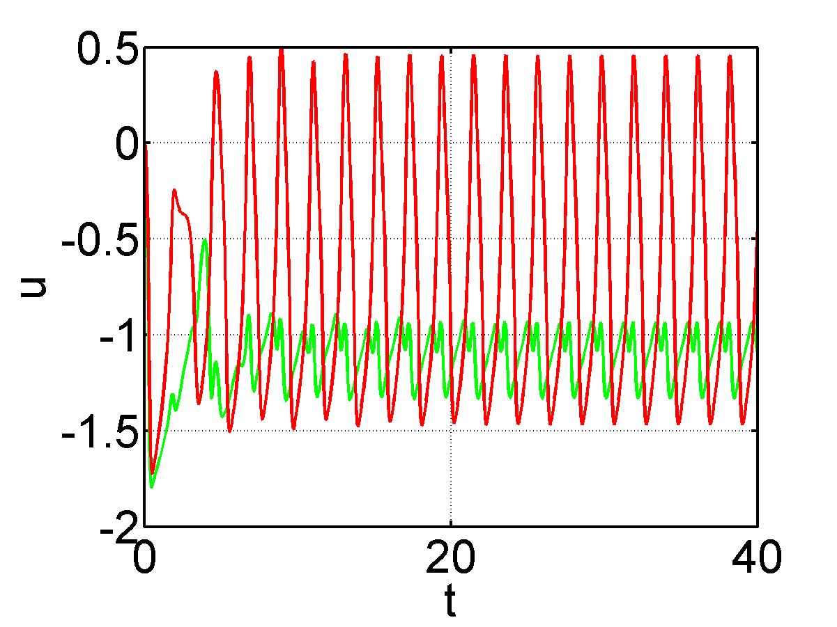
(a)

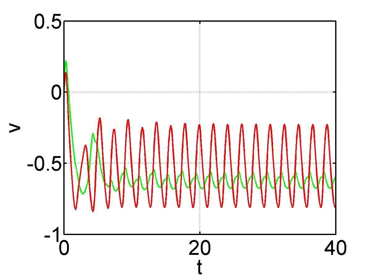
(b)

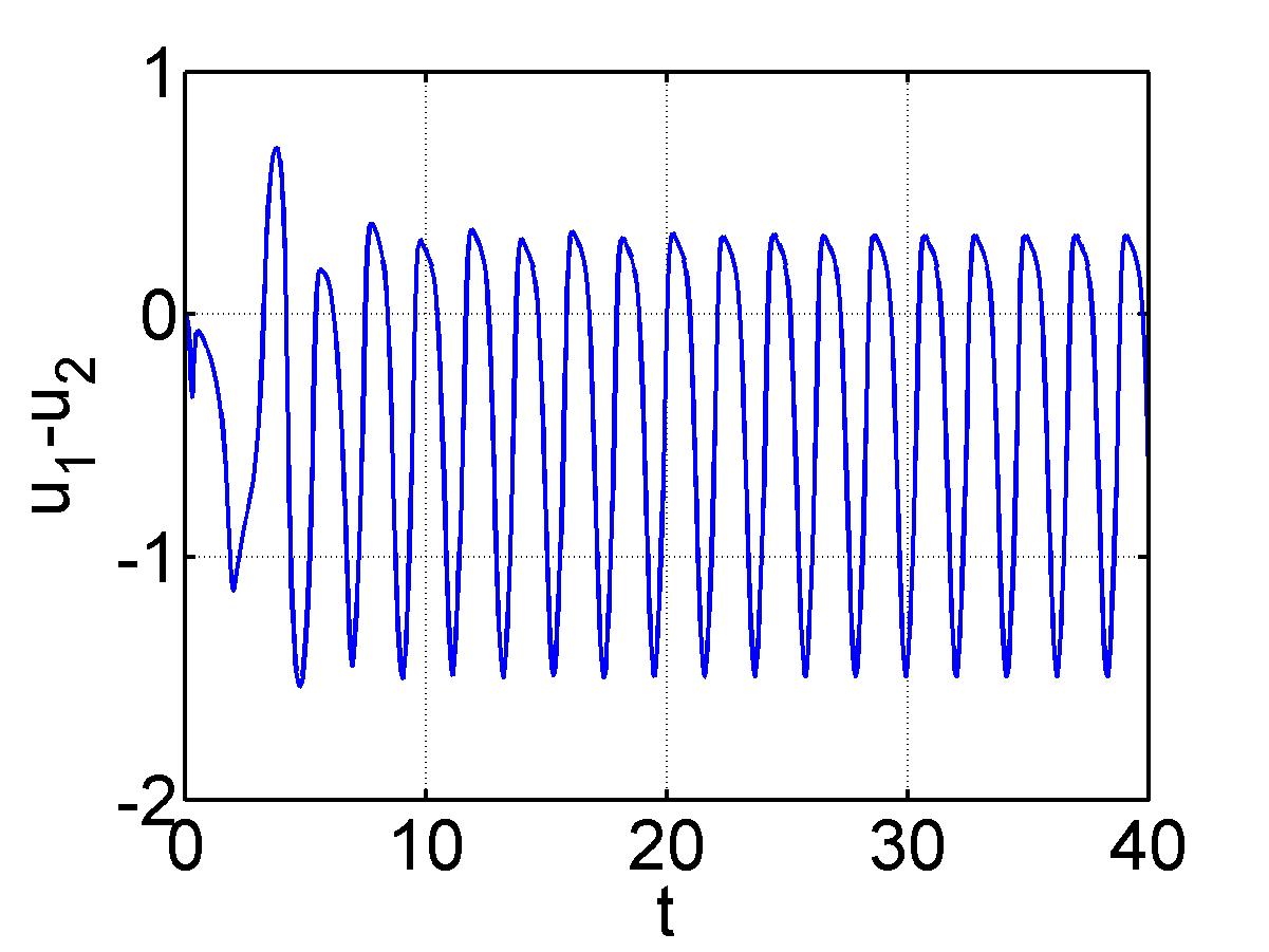
(c)

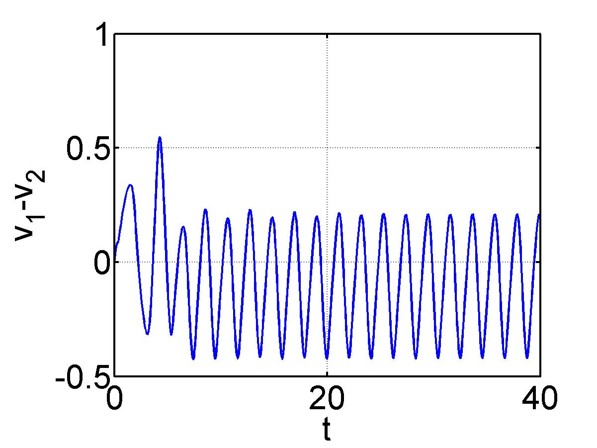
(d)

Figure 4: As in Fig. LABEL:fig2 but with smaller adaptation gain $\gamma=0.025$. Gray (green) line marks node one, black (red) line marks node two. (a) and (b): time series of the activator and the inhibitor, respectively; (c) and (d): differences $u_{1}-u_{2}$ and $v_{1}-v_{2}$ between the activator and the inhibitor values, respectively.

For constant coupling strength, i.e., $\gamma=0$, the two coupled FHN systems do not synchronize in-phase, but approach an anti-phase synchronized state: Figure LABEL:fig1 shows in panels (a) and (b) the time series of the activators and the inhibitors, respectively, and in panel (d) the phase portrait. Though the first node is in the excitable regime ($a_{1}=1.1>1$) both nodes oscillate due to the nonzero coupling strength $C$. However, they do not synchronize as can clearly be seen in panel (c) which depicts the difference $u_{1}-u_{2}$ between the activator values. Instead, they phase lock with a phase shift of approximately $\pi$ which corresponds to an anti-phase synchronized state.

We now adapt the coupling strength according to Eq. (20) in order to synchronize the two systems where the result is shown in Fig. LABEL:fig2. After a transient time of approximately 15 units of time the two systems reach the desired synchronized state (see the time series of the activator in Fig. LABEL:fig2(a) and the difference between its values Fig. LABEL:fig2(c)). Thus, the control is successful.

If the gain $\gamma$ is chosen too low the control fails: Figure 4 depicts the results of the adaptive control according to Eq. (20) for $\gamma=0.05$. Clearly, the control does not succeed in synchronizing the two systems (see the time series of the activators in Fig. 4(a) and the difference between their values in (c)).

The adaptive controller (19) ensures synchronization of the activators with a shift given by $a_{2}-a_{1}$ (see Eq. (18a)). Furthermore, there is a finite, constant shift in the inhibitor values (see Eq. (18b)). The shift in the inhibitor values can be reduced to a value close to zero if we control the coupling strength of each node separately. The two FHN systems are then described by

$$\varepsilon\dot{u_{i}} =u_{i}-\frac{u_{i}^{3}}{3}-v_{i}+C_{i}(t)[u_{(i+1)\bmod 2}(t-\tau)-u_{i}(t)],$$ (21)

$$\dot{v_{i}} =u_{i}+a_{i},\quad i=1,2$$

where $C_{i}(t)$ describes the strength of the coupling to node $i$. From Eq. (5) with $\mathbf{g}=(C_{1},C_{2})$, system (21), goal function (17), and $\psi(\mathbf{x},\mathbf{g},t)=\gamma\nabla_{\mathbf{g}}\omega(\mathbf{x},\mathbf{g},t)$ an adaptive law is straightforwardly derived:

$$C_{i}(t)=C_{i}^{0}+\frac{\gamma}{\varepsilon}\left[u_{i}(t)-u_{(i+1)\bmod 2}(t)+a_{i}-a_{(i+1)\bmod 2}\right]\left[u_{i}(t)-u_{(i+1)\bmod 2}(t-\tau)\right],\quad i=1,2$$ (22)

where $\gamma>0$ is the gain and $C_{i}^{0}$ is the initial value of control parameter.

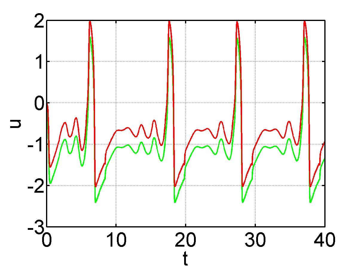
(a)

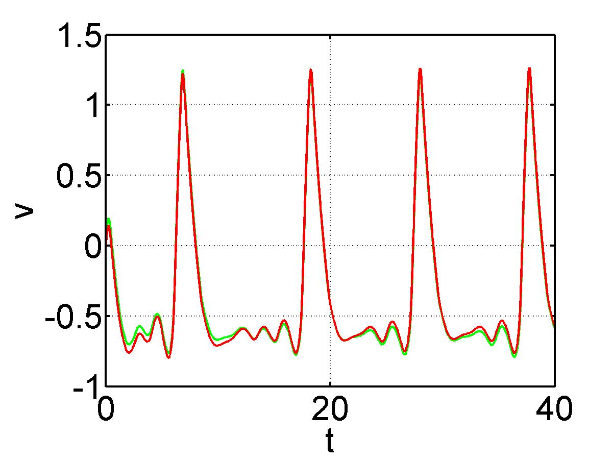
(b)

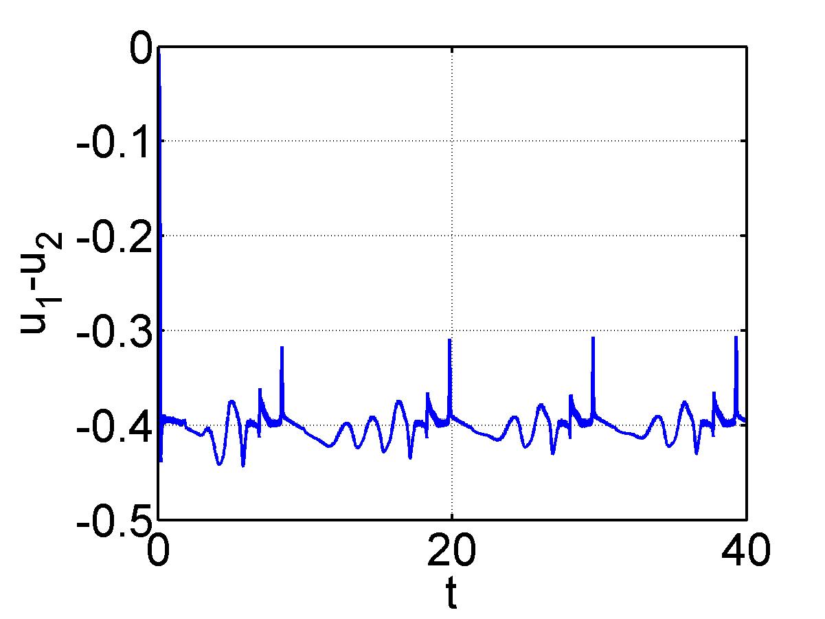
(c)

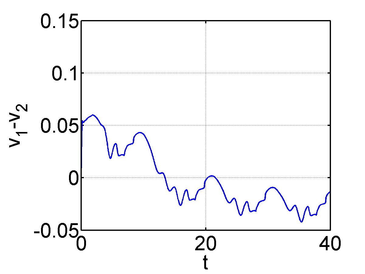
(d)

Figure 5: Adaptive control of two coupled FitzHugh-Nagumo systems (Eq. (21)) where the coupling strength $C_{i}$ of each node is adapted separately according to Eq. (22). Gray (green) line marks node one, black (red) line marks node two. (a) and (b): time series of the activator and the inhibitor, respectively; (c) and (d): differences $u_{1}-u_{2}$ and $v_{1}-v_{2}$ between the activator and the inhibitor values, respectively. Parameters: $\gamma=2$, $C_{i}^{0}=0$, $i=1,2$. Other parameters and initial conditions as in Fig LABEL:fig1.

The results of the adaptation according to Eq. (22) are shown in Fig. 5. The two systems reach the desired synchronized state (see the time series of the activators in Fig. 5(a) and the difference between their values in Fig. 5(c)). Moreover, the difference between inhibitor values is close to zero (see the time series of the inhibitors in Fig. 5(b) and the difference between their values in Fig. 5(d)). Thus, the control is successful.

5 Adaptive Synchronization in ring networks

We now want to apply our method to larger networks. To this end, we consider a ring network of $N$ nodes where the coupling matrix $\mathbf{G}$ has the following form

$$\mathbf{G}=\begin{pmatrix}0&1&0&\cdots&0\\ 0&0&1&\cdots&0\\ \vdots&\vdots&\ddots&\ddots&\vdots\\ 0&0&\ddots&\ddots&1\\ 1&0&0&\cdots&0\end{pmatrix}.$$ (23)

Our approach aims to synchronize two nodes of the ring; in this case the other nodes will follow these two nodes and synchronize as well. The same idea has been used in the control of wave motion in a chain of pendulums Fradkov & Andrievsky [2008]. However, there is a limitation to this approach: The nodes with the highest threshold and the lowest one have to be neighbors.

Let us assume that $k$ is the node with the highest threshold and $l$ is the one with the lowest threshold, i.e,

$$a_{k}=\max\limits_{i=1,\dots,N}a_{i},\qquad a_{l}=\min\limits_{i=1,\dots,N}a_{i},$$

and that $a_{k}$ and $a_{l}$ are neighbors, i.e., $k=(l+1)\bmod N$ or $k=(l-1)\bmod N$.

We now use the adaptation law (20) to synchronize these two nodes. With nodes $k$ and $l$ instead of nodes $1$ and $2$, Eq. (20) reads

$$C(t)=C_{0}+\frac{\gamma}{\varepsilon}\left[u_{k}(t)-u_{l}(t)+a_{k}-a_{l}\right]\left[u_{k}(t)-u_{l}(t)\right],$$ (24)

where $\gamma$ is the gain and $C_{0}$ is an initial value of the coupling strength. As before, we aim to achieve the control goal (2). Similar to the case of two coupled FHN systems, the control (24) ensures synchronization in a nearly synchronized state characterized by

$$u_{i}(t)-u_{j}(t) \approx -a_{i}+a_{j},$$ (25a)

$$v_{i}(t)-v_{j}(t) \approx c_{i},$$ (25b)

for $t\geqslant t^{*}$, where $c_{i}$ is constant and $i,j=1,\ldots,N$.

Figure LABEL:fig4 presents the results of a simulation of ten FitzHugh-Nagumo systems coupled in a ring where the adaption law (24) is applied with $a_{1}=a_{k}$ being the node with the highest threshold, and $a_{2}=a_{l}$ being the node with the lowest threshold. In Fig. LABEL:fig4(a) and LABEL:fig4(c), it is shown that activators $u_{1}$ and $u_{2}$ synchronize. Figure LABEL:fig4(e) shows the phase space of the two nodes. In Fig. LABEL:fig4(g) it can be seen that not only node one and two are synchronized but that all nodes follow these two nodes and synchronize after a transient time. Thus, the control goal is achieved.

Figure LABEL:fig4(f) shows that there are several jumps in the control $C$ during the transient time and that $C$ temporarily reaches quite high values. To avoid this, we can limit the coupling strength $C$. Figure LABEL:fig5 presents the results for a bounded coupling strength, i.e., $|C|\leqslant 5$. The control is successful; however, the transient time is prolonged compared to the unbounded control shown in Fig. LABEL:fig4(g).

So far we considered the case that the nodes with the highest and lowest coupling strength are neighbors. If this is not fulfilled, the adaptation of the overall coupling strength does not yield synchronization. However, if we control the coupling strength of each node separately the control goal can be reached. The ring network is then described by

$$\varepsilon\dot{u_{i}} =u_{i}-\frac{u_{i}^{3}}{3}-v_{i}+C_{i}(t)[u_{(i+1)\bmod N}(t-\tau)-u_{i}(t)],$$ (26)

$$\dot{v_{i}} =u_{i}+a_{i},\quad i=1,\dots,N,$$

where $C_{i}(t)$ describes the strength of the coupling to node $i$. As in the case of two nodes, from Eq. (5) with $\mathbf{g}=(C_{1},\ldots,C_{N})$, goal function

$$Q(\mathbf{x}(t),t)= \frac{1}{2}\sum_{i=1}^{N}\left[u_{i}(t)-u_{(i+1)\bmod N}(t)+a_{i}-a_{(i+1)\bmod N}\right]^{2},$$ (27)

and

$$\psi(\mathbf{x},\mathbf{g},t) = \gamma\nabla_{\mathbf{g}}\omega(\mathbf{x},\mathbf{g},t),$$ (28)

we derive the following adaption law

$$C_{i}(t)= C_{i}^{0}+\frac{\gamma}{\varepsilon}\left[u_{i}(t)-u_{(i+1)\bmod N}(t-\tau)\right]$$ (29)

$$\times\big{[}2u_{i}(t)-u_{(i-1)\bmod N}(t)-u_{(i+1)\bmod N}(t)+2a_{i}-a_{(i-1)\bmod N}(t)-a_{(i+1)\bmod N}(t)\big{]},\,i=1,\dots,N,$$

where $\gamma$ is the gain and $C_{i}^{0}$ is the initial value of $C_{i}$.

Figure LABEL:fig6 presents the results of a simulation of Eq. (26) with adaption law (29). The control goal is achieved and synchronization takes place. This method requires a lower gain than algorithm (24), and, moreover, it ensures synchronization of the inhibitors with a negligible shift (see the time series of the inhibitors in Fig. LABEL:fig6(b)).

6 Conclusion

We have proposed a novel adaptive method for controlling synchrony in heterogeneous networks. It is well known that networks with heterogeneous nodes are much less likely to synchronize than networks of identical nodes. Furthermore, synchrony will take place in a state where the trajectories of the different nodes are not identical but small deviations can be observed. We have suggested a goal function to characterize this type of synchrony. Based on this goal function and the speed-gradient (SG) method, we have derived an adaptive controller which tunes the overall coupling strength such that synchrony is stable despite the node heterogeneities.

We have demonstrated our method on networks of FitzHugh-Nagumo systems, a neural model which is considered to be generic for excitable systems close to a Hopf bifurcation. Before applying the adaptive control, we have studied the simple motif of two delay-coupled, heterogeneous nodes and have given analytic conditions for the occurrence of the Hopf bifurcations. We have then applied our adaptive method and discussed its dependencies on the node and control parameters. It has been shown that our method enables synchronization even if the node parameters are chosen such diverse that one of the systems would exhibit self-sustained oscillations without coupling, while the other one would remain in a stable equilibrium point, i.e., one of the uncoupled systems is above, and the other is below the Hopf bifurcation. Furthermore, we have generalized our method to larger networks and applied it to ring networks. As an alternative and complement to adapting the overall coupling strength, we have suggested adapting the coupling strength of each node separately. This allows for adaptively controlling the network in situations where the node with the highest threshold is not a direct neighbor of the node with the lowest threshold, in contrast to the restriction imposed by tuning only the overall coupling strength.

Here, we have considered static delays. In principle, it would be possible to extend the method to time varying delays. Time varying delay in neural networks has been considered in Refs. Wang et al. [2008]; Tang et al. [2008]; Li et al. [2014]. In general networks time varying delay has been studied in Refs. Yu et al. [2008]; Gjurchinovski et al. [2014]. However, to our knowledge no adaptive control methods have been applied in networks with time varying delay and heterogeneous nodes.

Given the paradigmatic nature of the FitzHugh-Nagumo system, we expect our method to be applicable in a wide range of excitable systems. Furthermore, the application of the SG method to the control of networks with heterogeneous nodes suggests that other adaptive controllers that are based on the SG method (see, for example, Refs. Selivanov et al. [2012]; Schöll et al. [2012]; Guzenko et al. [2013]; Lehnert et al. [2014]) are also robust towards heterogeneities.

Acknowledgments

This work is supported by the German-Russian Interdisciplinary Science Center (G-RISC) funded by the German Federal Foreign Office via the German Academic Exchange Service (DAAD). J.L. and E.S. acknowledge support by Deutsche Forschungsgemeinschaft (DFG) in the framework of SFB 910. S.P. and A.F. acknowledge that Sec. 4.1 was performed in IPME RAS, supported solely by RSF (Grant No. 14-29-00142).

References

- Bachmair & Schöll [2014] Bachmair, C. A. & Schöll, E. [2014] “Nonlocal control of pulse propagation in excitable media,” Eur. Phys. J. B 87, 276, 10.1140/epjb/e2014-50339-2.
- Brandstetter et al. [2010] Brandstetter, S. A., Dahlem, M. A. & Schöll, E. [2010] “Interplay of time-delayed feedback control and temporally correlated noise in excitable systems,” Phil. Trans. R. Soc. A 368, 391.
- Cakan et al. [2014] Cakan, C., Lehnert, J. & Schöll, E. [2014] “Heterogeneous delays in neural networks,” Eur. Phys. J. B 87, 54, 10.1140/epjb/e2014-40985-7.
- Chen [2014] Chen, Z. [2014] “Pattern synchronization of nonlinear heterogeneous multiagent networks with jointly connected topologies,” IEEE Trans. Control Network Syst. 1, 349–359, 10.1109/tcns.2014.2357551.
- Dahlem et al. [2009] Dahlem, M. A., Hiller, G., Panchuk, A. & Schöll, E. [2009] “Dynamics of delay-coupled excitable neural systems,” Int. J. Bifur. Chaos 19, 745–753.
- DeLellis et al. [2015] DeLellis, P., di Bernardo, M. & Liuzza, D. [2015] “Convergence and synchronization in heterogeneous networks of smooth and piecewise smooth systems,” Automatica 56, 1–11, 10.1016/j.automatica.2015.03.003.
- FitzHugh [1961] FitzHugh, R. [1961] “Impulses and physiological states in theoretical models of nerve membrane,” Biophys. J. 1, 445.
- Flunkert et al. [2010] Flunkert, V., Yanchuk, S., Dahms, T. & Schöll, E. [2010] “Synchronizing distant nodes: a universal classification of networks,” Phys. Rev. Lett. 105, 254101, 10.1103/physrevlett.105.254101.
- Fradkov [1979] Fradkov, A. L. [1979] “Speed-gradient scheme and its application in adaptive control problems,” Autom. Remote Control 40, 1333–1342.
- Fradkov [2007] Fradkov, A. L. [2007] Cybernetical Physics: From Control of Chaos to Quantum Control (Springer, Heidelberg, Germany).
- Fradkov & Andrievsky [2008] Fradkov, A. L. & Andrievsky, B. [2008] “Control of wave motion in the chain of pendulums,,” Proc. 17th IFAC World Congress, Seoul 17, 3136–3141.
- Fradkov & Junussov [2013] Fradkov, A. L. & Junussov, I. A. [2013] “Decentralized adaptive controller for synchronization of nonlinear dynamical heterogeneous networks,” Int. J. Adapt. Control Signal Process 27, 729–740, 10.1002/acs.2343.
- Fries [2005] Fries, P. [2005] “A mechanism for cognitive dynamics: Neuronal communication through neuronal coherence,” Trends in Cognitive Sciences 9, 474–480, cited By 880.
- Gjurchinovski et al. [2014] Gjurchinovski, A., Zakharova, A. & Schöll, E. [2014] “Amplitude death in oscillator networks with variable-delay coupling,” Phys. Rev. E 89, 032915, 10.1103/physreve.89.032915.
- Guo & Li [2013] Guo, X. & Li, J. [2013] “Stochastic adaptive synchronization for time-varying complex delayed dynamical networks with heterogeneous nodes,” Appl. Math. Comput. 222, 381–390, 10.1016/j.amc.2013.07.030.
- Guzenko et al. [2013] Guzenko, P. Y., Lehnert, J. & Schöll, E. [2013] “Application of adaptive methods to chaos control of networks of Rössler systems,” Cybernetics and Physics 2, 15–24.
- Heinrich et al. [2010] Heinrich, M., Dahms, T., Flunkert, V., Teitsworth, S. W. & Schöll, E. [2010] “Symmetry breaking transitions in networks of nonlinear circuit elements,” New J. Phys. 12, 113030, 10.1088/1367-2630/12/11/113030.
- Hövel et al. [2010] Hövel, P., Dahlem, M. A. & Schöll, E. [2010] “Control of synchronization in coupled neural systems by time-delayed feedback,” Int. J. Bifur. Chaos 20, 813–815.
- Isidori et al. [2014] Isidori, A., Marconi, L. & Casadei, G. [2014] “Robust output synchronization of a network of heterogeneous nonlinear agents via nonlinear regulation theory,” IEEE Trans. Autom. Control 59, 2680–2691, 10.1109/tac.2014.2326213.
- Izhikevich [2000] Izhikevich, E. M. [2000] “Neural excitability, spiking, and bursting,” Int. J. Bifurcation Chaos 10, 1171–1266.
- Lehnert et al. [2011] Lehnert, J., Dahms, T., Hövel, P. & Schöll, E. [2011] “Loss of synchronization in complex neural networks with delay,” Europhys. Lett. 96, 60013, 10.1209/0295-5075/96/60013.
- Lehnert et al. [2014] Lehnert, J., Hövel, P., Selivanov, A. A., Fradkov, A. L. & Schöll, E. [2014] “Controlling cluster synchronization by adapting the topology,” Phys. Rev. E 90, 042914, 10.1103/physreve.90.042914.
- Li et al. [2014] Li, Y., Li, J. & Hua, M. [2014] “New results of h∞ filtering for neural network with time-varying delay,” IJICIC 10.
- Lindner et al. [2004] Lindner, B., García-Ojalvo, J., Neiman, A. B. & Schimansky-Geier, L. [2004] “Effects of noise in excitable systems,” Phys. Rep. 392, 321–424.
- Lu et al. [2015] Lu, C. H., Tai, C. C., Chen, T. C. & Wang, W. C. [2015] “Fuzzy neural network speed estimation method for induction motor speed sensorless control,” IJICIC 11, 433–445.
- Lu et al. [2012] Lu, J., Kurths, J., Cao, J., Mahdavi, N. & Huang, C. [2012] “Synchronization control for nonlinear stochastic dynamical networks: Pinning impulsive strategy,” IEEE Trans. Neural Netw. Learn. Syst. 23, 285–292.
- Lu & Qin [2009] Lu, X. & Qin, B. [2009] “Adaptive cluster synchronization in complex dynamical networks,” Phys. Lett. A 373, 3650–3658, 10.1016/j.physleta.2009.08.013.
- Murray [1993] Murray, J. D. [1993] Mathematical Biology, Biomathematics Texts, Vol. 19, 2nd ed. (Springer, Berlin Heidelberg).
- Nagumo et al. [1962] Nagumo, J., Arimoto, S. & Yoshizawa., S. [1962] “An active pulse transmission line simulating nerve axon.” Proc. IRE 50, 2061–2070.
- Omelchenko et al. [2011] Omelchenko, I., Maistrenko, Y., Hövel, P. & Schöll, E. [2011] “Loss of coherence in dynamical networks: spatial chaos and chimera states,” Phys. Rev. Lett. 106, 234102, 10.1103/physrevlett.106.234102.
- Panchuk et al. [2013] Panchuk, A., Rosin, D. P., Hövel, P. & Schöll, E. [2013] “Synchronization of coupled neural oscillators with heterogeneous delays,” Int. J. Bifurcation Chaos 23, 1330039, 10.1142/s0218127413300395.
- Pikovsky et al. [2003] Pikovsky, A., Rosenblum, M. & Kurths, J. [2003] Synchronization: A universal concept in nonlinear sciences, Vol. 12 (Cambridge Univerity Press, Cambridge).
- Poeck & Hacke [2001] Poeck, K. & Hacke, W. [2001] Neurologie, 11th ed. (Springer, Heidelberg).
- Postlethwaite et al. [2013] Postlethwaite, C. M., Brown, G. & Silber, M. [2013] “Feedback control of unstable periodic orbits in equivariant hopf bifurcation problems,” Phil. Trans. R. Soc. A 371, 20120467, 10.1098/rsta.2012.0467.
- Ricci et al. [2012] Ricci, F., Tonelli, R., Huang, L. & Lai, Y.-C. [2012] “Onset of chaotic phase synchronization in complex networks of coupled heterogeneous oscillators,” Phys. Rev. E 86, 027201, 10.1103/physreve.86.027201.
- Schöll et al. [2009] Schöll, E., Hiller, G., Hövel, P. & Dahlem, M. A. [2009] “Time-delayed feedback in neurosystems,” Phil. Trans. R. Soc. A 367, 1079–1096, 10.1098/rsta.2008.0258.
- Schöll & Schuster [2008] Schöll, E. & Schuster, H. G. (eds.) [2008] Handbook of Chaos Control (Wiley-VCH, Weinheim), second completely revised and enlarged edition.
- Schöll et al. [2012] Schöll, E., Selivanov, A. A., Lehnert, J., Dahms, T., Hövel, P. & Fradkov, A. L. [2012] “Control of synchronization in delay-coupled networks,” Int. J. Mod. Phys. B 26, 1246007, 10.1142/s0217979212460071.
- Selivanov et al. [2012] Selivanov, A. A., Lehnert, J., Dahms, T., Hövel, P., Fradkov, A. L. & Schöll, E. [2012] “Adaptive synchronization in delay-coupled networks of Stuart-Landau oscillators,” Phys. Rev. E 85, 016201, 10.1103/physreve.85.016201.
- Shi et al. [2015] Shi, P., Zhang, Y., Chadli, M. & Agarwal, R. K. [2015] “Mixed h-infinity and passive filtering for discrete fuzzy neural networks with stochastic jumps and time delays,” IEEE Trans. Neural Networks Learn. Syst. PP, 1, 10.1109/tnnls.2015.2425962.
- Shiriaev & Fradkov [2000] Shiriaev, A. S. & Fradkov, A. L. [2000] “Stabilization of invariant sets for nonlinear non-affine systems,” Automatica 36, 1709–1715, doi: 10.1016/s0005-1098(00)00077-7.
- Singer [1999] Singer, W. [1999] “Neuronal Synchrony: A Versatile Code Review for the Definition of Relations?” Neuron 24, 49–65.
- Strogatz [2000] Strogatz, S. H. [2000] “From Kuramoto to Crawford: exploring the onset of synchronization in populations of coupled oscillators,” Physica D 143, 1–20.
- Sun et al. [2009] Sun, J., Bollt, E. M. & Nishikawa, T. [2009] “Master stability functions for coupled nearly identical dynamical systems,” Europhys. Lett. 85, 60011.
- Sun & Ding [2013] Sun, J. Q. & Ding, G. [2013] Advances in Analysis and Control of Time-Delayed Dynamical Systems (World Scientific, Singapore), ISBN 978-981-4522-02-1.
- Tang et al. [2008] Tang, Y., Qiu, R., Fang, J.-a., Miao, Q. & Xia, M. [2008] “Adaptive lag synchronization in unknown stochastic chaotic neural networks with discrete and distributed time-varying delays,” Phys. Lett. A 372, 4425–4433, 10.1016/j.physleta.2008.04.032.
- Tass et al. [1998] Tass, P. A., Rosenblum, M. G., Weule, J., Kurths, J., Pikovsky, A., Volkmann, J., Schnitzler, A. & Freund, H. J. [1998] “Detection of n:m phase locking from noisy data: Application to magnetoencephalography,” Phys. Rev. Lett. 81, 3291.
- Uhlhaas et al. [2009] Uhlhaas, P., Pipa, G., Lima, B., Melloni, L., Neuenschwander, S., Nikolic, D. & Singer, W. [2009] “Neural synchrony in cortical networks: history, concept and current status,” Front. Integr. Neurosci. 3, 17, 10.3389/neuro.07.017.2009.
- Wang et al. [2008] Wang, K., Teng, Z. & Jiang, H. [2008] “Adaptive synchronization of neural networks with time-varying delay and distributed delay,” Physica A 387, 631–642, 10.1016/j.physa.2007.09.016.
- Yu et al. [2008] Yu, W., Cao, J. & Lü, J. [2008] “Global synchronization of linearly hybrid coupled networks with time-varying delay,” SIAM J. Appl. Dyn. Syst. 7, 108–133, 10.1137/070679090.
- Zhou et al. [2008] Zhou, J., Lu, J. a. & Lü, J. [2008] “Pinning adaptive synchronization of a general complex dynamical network,” Automatica 44, 996.