Ideological and Temporal Components of Network Polarization in Online Political Participatory Media

Abstract

Political polarization is traditionally analyzed through the ideological stances of groups and parties, but it also has a behavioral component that manifests in the interactions between individuals. We present an empirical analysis of the digital traces of politicians in politnetz.ch, a Swiss online platform focused on political activity, in which politicians interact by creating support links, comments, and likes. We analyze network polarization as the level of intra-party cohesion with respect to inter-party connectivity, finding that supports show a very strongly polarized structure with respect to party alignment. The analysis of this multiplex network shows that each layer of interaction contains relevant information, where comment groups follow topics related to Swiss politics. Our analysis reveals that polarization in the layer of likes evolves in time, increasing close to the federal elections of 2011. Furthermore, we analyze the internal social network of each party through metrics related to hierarchical structures, information efficiency, and social resilience. Our results suggest that the online social structure of a party is related to its ideology, and reveal that the degree of connectivity across two parties increases when they are close in the ideological space of a multi-party system.

1 Introduction

Political polarization is an important ingredient in the functioning of a democratic system, but too much of it can lead to gridlock or even violent conflict. An excess of political homogeneity, on the other hand, may render democratic choice meaningless (Sunstein, 2003). It is therefore of fundamental interest to understand the factors shifting this delicate balance to one of the two extremes. Consequently, polarization has long been a central topic for political science. Within this article, we build on this tradition, but we also want to supplement it with several currently rather unregarded aspects. First, large parts of political polarization literature are concerned with two-party systems, particularly in the context of the United States (Waugh et al., 2009). And second, polarization is generally conceptualized on the basis of positions in ideological space (Hetherington, 2009). Commonly used measures of political polarization are derived from those two premises, and therefore conceptualize polarization as two ideological blocks (i.e. parties) drifting apart on one political dimension, while increasing their internal agreement.

Many democratic systems are characterized by more than two relevant parties, making it problematic to apply standard ideology-based measures of polarization to them (Waugh et al., 2009). Besides methodological concerns, we argue that an exclusive focus on ideological positions does not capture all aspects of the term polarization. It has been claimed that a sensible definition of polarization would have to comprise not only the ideological stances of the polarized set of individuals or parties, but also the interactions between them (Blau, 1977; Baldassarri and Bearman, 2007; Conover et al., 2011; Gruzd and Roy, 2014). At the same level of ideological polarization, we would ascribe a higher level of polarization to a set of political actors when: i) they display a bias towards positive interaction between actors of similar political positions, and ii) they tend towards negative interaction between actors with dissimilar political positions (Guerra et al., 2013; Gruzd and Roy, 2014). Assuming a feedback between opinion and network polarization, a polarized society is divided into by a small number of groups with high internal consensus and sharp disagreement between them (Flache and Macy, 2011). When establishing a social link means to agree on opinions to certain extent (Guerra et al., 2013), network polarization is defined as a phenomenon in which the underlying social network of a society is composed of highly connected subgroups with weak inter-group connectivity (Conover et al., 2012; Guerra et al., 2013). The terms clusters, modules or communities are often used as synonyms to define groups of individuals in a (social) network based on their link topology. Such assignments are usually not unique, i.e. individuals can be counted in different communities. Various algorithms for network partitioning exist to optimize this assignment, often based on the optimization of modularity metrics (Newman, 2006). By adopting a network science approach, we are able to capture and analyse the interaction aspect of polarization, and at the same time to expand the study of polarization to multi-party systems. In this work, we focus on the network of support and interaction among politicians only. This way, our analysis is performed within the context of elite polarization (Fiorina and Abrams, 2008; Hetherington, 2009), as a complementary view to previous studies of mass polarization through blogs and Twitter (Guerra et al., 2013; Gruzd and Roy, 2014).

Online political participatory media, like opencongress.org and politnetz.ch, serve as a digital representation of a political system where voters and politicians can discuss in an online medium. These political participatory media serve as crowdsourcing platforms for the proposal and discussion of policies, leaving digital traces that allow unprecedented quantitative analyses of political interaction. In this study, we present our analysis of politnetz.ch, a Swiss platform that allowed us to obtain data about online political participation. On politnetz.ch, politicians and citizens freely discuss political topics, and also weave a social network around them by expressing their support for politicians or by liking each others’ contributions. Though politnetz.ch is of course subject to many limitations and distortions, it can be seen as a fairly faithful online representation of Swiss politics. The plurality of Swiss politics allows us to study polarization along party, as well as along ideological lines. Additionally, the real-time quality of politnetz.ch data enables us to analyze polarization with a very high temporal resolution. While traditional research mainly focuses on changes in polarization within years or decades (McCarty et al., 2006), we can detect them within the scope of days and weeks. This makes it possible to quantify the influence of day-to-day political events, such as elections and referendums (which are of particular relevance in Swiss politics (Serdült, 2014)).

Previous works on the dynamics of polarization use agent-based modelling approaches to simulate and analyze polarization in opinion dynamics. Here, we can distinguish between two different model classes. First, models with binary opinions, often called voter models, already imply that these are opposite opinions. The question is then about the share of opposite opinions in a population of agents (Schweitzer and Behera, 2009). Some scenarios show the emergence of a majority favoring one opinion, or even the convergence of the whole population toward the same opinion, called consensus. A polarization scenario in binary opinion models results in the coexistence of opposite opinions, often with almost equal share. Second, models with continuous opinions focus on the (partial) convergence of “neighboring” opinions such that groups of agents with the same opinion emerge. Polarization in such models can occur if two of these groups coexist, without any possibility to reach consensus (Groeber et al., 2009). In most cases, opinion dynamics models assume an interaction between opinions and the underlying communication structure, with agents of similar opinions communicating more frequently with each other than with dissimilar agents. This can be a result of homophily (i.e., opinion difference influencing structure) or of social influence (structure influencing opinion). We will explore if those model assumptions also hold in the empirical social network of politnetz.ch.

Online participatory media offer different possibilities of interaction between individuals. Online actions, such as creating a social link or commenting on a post, can be used in different context. Nevertheless, interdependencies might exist between these interaction types. For example, if users press the like button only to posts they positively comment, the liking action would not contribute additional information to the communication process. In this work, one of our goals is to quantify how much information about one interaction type is contained in another, assessing the added value of including all these interaction types in the analysis of online communities. In our analysis, we explore the three main interaction types between politicians in politnetz.ch: supports, likes, and comments, to measure the differences of politicians’ behavior in each interaction context. For instance, do politicians only like posts of politicians they support? Do the patterns of support among politicians project onto comments and likes? In our analysis, we aim to discover groups of politicians determined by the networks of supports, likes and comments, and not necessarily by their party affiliation. It might be the case that two politicians that are the members of the same party, might not support each other, and conversely, it can be the case that two politicians that are not the members of the same party do support each other. How often do such scenarios occur? Does the party affiliation of a politician define whom they support, like, and comment, producing network polarization?

Previous works centered around the US found strong polarization between left- and right-leaning politicians (Saunders and Abramowitz, 2004). However, left- and right- leaning attitudes generally coincide with party membership in the US two-party system. This way, it cannot be distinguished whether polarization is created along the left-right dimension or along party lines, which can only be differentiated in a multi-party system. The US left- and right-aligned communities also differ in their online interaction, as shown in previous works using blogs (Adamic and Glance, 2005), Twitter (Conover et al., 2012), and Youtube (Garcia et al., 2012), opening the question of whether these patterns prevail in other countries. We analyze the network topology of politnetz.ch, its evolution over time, and the topologies the social networks within each party. As a consequence, we characterize the role of elections and party ideology in network polarization, both at the party and at the global level. The fact that most politicians in politnetz.ch clearly state their party membership and make their online interaction with other politicians via likes, supports, comments publicly available, allows us to test the following hypotheses: i) political polarization is present in layers with a positive connotation, i.e. supports and likes, ii) polarization, if present, is not solely grounded upon political party alignment, but also depends on politically relevant events, such as elections, and on the distance between parties in ideological space.

Finally, we ask the question of whether the social structure of parties is related to their ideology. Previous research in the US political system showed differences in online network topology between the right- and left-aligned groups (Conover et al., 2012). This opens questions whether i) there are differences in the party structures of the political systems with more than two parties, and whether ii) the pattern in the US for right- and left- subcommunities holds in a multi-party system. We study Switzerland as an example of a country with a multi-party political system, with the presence of major and minor parties and additional ideological dimensions beyond left and right.

2 Materials and methods

2.1 Politnetz data

Politnetz.ch is an online platform that enhances communication among politicians and voters in Switzerland. Profiles in politnetz.ch are registered either for voters or politicians, where politician profiles have an additional section called “Political information”. This section includes the party a politician belongs to, selected from among valid parties in Switzerland. Registration as a politician on politnetz.ch is not verified by the platform, due to the fact that politicians are not motivated to misrepresent themselves. This becomes evident in their profile information: two thirds of the politician profiles include links to their homepages, while none of the voter profiles has an external website link.

With respect to the amount of politicians in Switzerland, politnetz.ch contains a large set of politician accounts, with a certain bias towards German-speaking regions. The amount of voter accounts is more limited with respect to the size of the electorate, and voters do not have any field for party affiliation in their profile. As mentioned above, we focus exclusively on politicians’ accounts, excluding voters accounts from all analyses.

Politicians have three major means of social interaction in politnetz.ch: i) they can support other politicians, ii) they can write posts and comments on the posts of other politicians, and iii) they can explicitly like posts, which are publicly displayed in their profile. Our politnetz.ch dataset includes the full track of interaction between politicians for more than two years, including 3441 politicians, which created 16699 support links, 45627 comments, and 10839 likes to posts. These digital traces are analogous to the the data of previous works on Twitter for US (Conover et al., 2012) and German politicians (Lietz et al., 2014), where follower relationships imitate support links, retweets resemble likes, and mentions are used as comments.

Analyzing politnetz.ch data provides a complementary approach to dominating Twitter-centric studies, which suffer of the model organism bias (Tufekci, 2014), in which the prevalence of Twitter as a data source can drive a scientific community to take platform-dependent findings as universal. Furthermore, politnetz.ch is richer as a data source compared to Twitter for three reasons: i) political alignment is explicit in and does not rely on external coding, ii) digital traces include all three layers of interaction, in contrast with Twitter data limitations that often leave out the follower network (Conover et al., 2011; Aragón et al., 2013; Gruzd and Roy, 2014), and iii) Politnetz provides information about the creation of support links, in contrast with Twitter’s opacity with respect to follower link creation times, forcefully simplifying the follower network as static (Conover et al., 2012; Lietz et al., 2014).

In our dataset, more than 80% of the politicians declare themselves as members of an existing party. We simplify the party affiliation data by merging local and youth versions of the same party, creating table in which each politician is mapped to one of the 9 parties, or left unaligned. The latter tag – “unaligned” politician – is an umbrella label for three distinct categories of political affiliation: 1.3% of the politicians stated they are independent politicians, 2.9% chose membership to non-governmental and nonprofit organizations, and the remaining 13% of the politicians who did not provide affiliation information to any party or organization, which in general are politicians active at the local level without alignment to any party at the federal level. In Table 1 we show the absolute count of politicians in the 9 parties and in the unaligned category.

Party	Description	N	Colour
SP	Social Democratic Party	609
SVP	Swiss People’s Party, incl. EDU	484
FDP	The Liberals	473
Christian	CSP, CVP, EVP	423
Grüne	Green Party	298
GLP	Green Liberal Party	286

Party	Description	N	Colour
BDP	Conservative Democratic Party	151
Piraten	Pirate Party	93
AL	Alternative Left, incl. PdA	28
	Unaligned	596
	Independent	47
	NGO/Union	101
	No affiliation	448

Table 1: Number of politicians in each of the 9 parties and in the unaligned category. Politicians labeled as unaligned can be further divided into three subgroups: independent politicians, NGO/NPO/trade union representatives, and politicians with no party affiliation. The fourth column shows colour codes of each of the 9 parties, which we use throughout this article.

2.2 Methods

Multiplex network analysis

The digital traces of politicians in politnetz.ch allow us to study interaction in three network layers, one composed of supports, a second one of likes, and a third one of comments. Every node belongs to each layer, and represents a politician with an account in politnetz.ch. A politician $p_{1}$ has a directed link to another politician $p_{2}$ in the supports layer if $p_{1}$ has $p_{2}$ in its list of supported politicians. The likes and comments layers are also directed, but in addition, links have weights equivalent to respectively the amount of likes and comments that $p_{1}$ gave to the posts and comments of $p_{2}$. These three layers compose a multiplex network, also known as a multimodal, multirelational or multivariate network, (Menichetti et al., 2014), as depicted in Figure 1. Multiplex networks are a subset of multilayered networks: Multiplex networks have one- to-one relationships between nodes across layers and multilayered networks have arbitrary connections across layers (Boccaletti et al., 2014). The paradigmatic example of a multiplex network is a social network with different types of social relationships (friendship, business, or family) (Szell et al., 2010). Examples of previously analyzed multiplex networks are air transportation networks, in which airports are connected through different airlines, (Cardillo et al., 2013), and online videogames where players can fight, trade, or communicate with each other, (Szell et al., 2010).

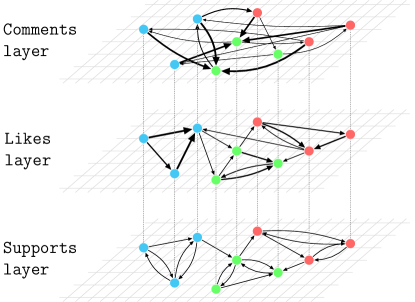
Figure 1: Three layers of the multiplex network in Politnetz.ch. The layer of supports is directed and unweighted, and the layers of likes and comments are directed and weighted. Node colors illustrate an party affiliation, and link widths are proportional to their weights.

The network layers are visualized in Figure 2, where nodes are colored according to their party alignment. Following the Fruchterman- Reingold layout algorithm (Fruchterman and Reingold, 1991), which locates connected nodes closer to each other, an initial observation of Figure 2 motivates our research question: politicians seem to be polarized along party lines when creating support links, while this pattern is not so clear for likes and comments.

(a) Supports layer, $|V|=2,740$, $|E|=16,657$

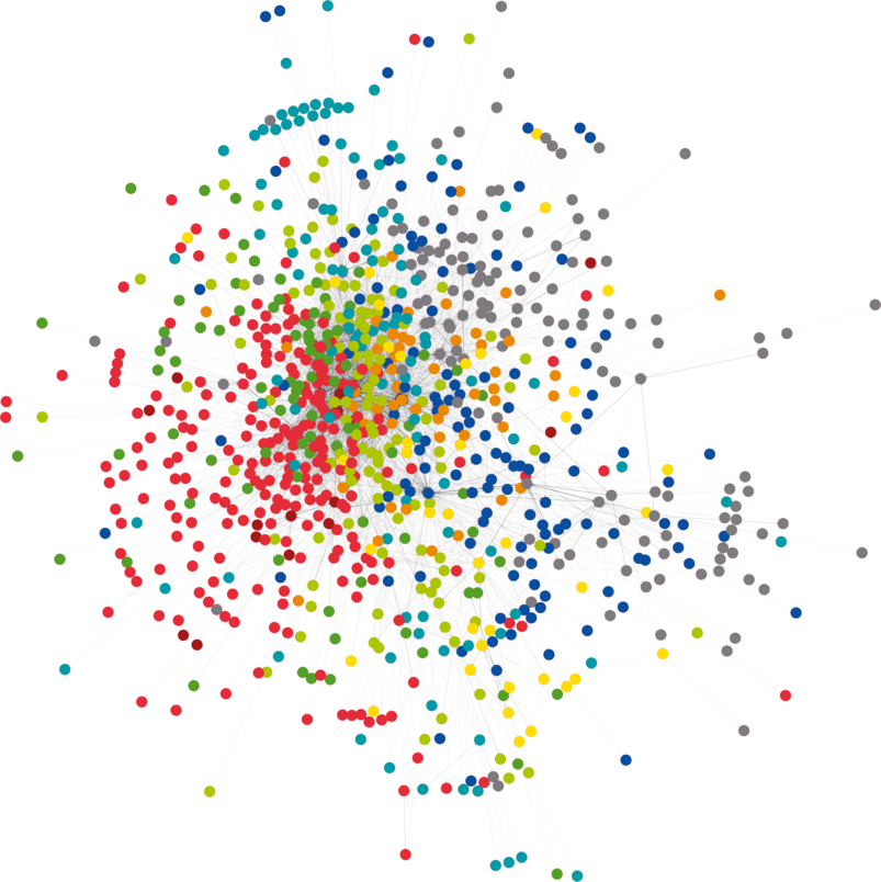
(b) Likes layer, $|V|=1,147$, $|E|=6,386$

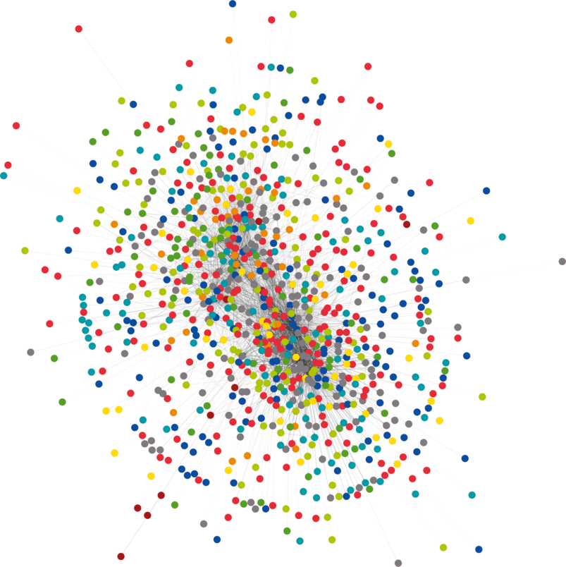
(c) Comments layer, $|V|=1,091$, $|E|=6,800$

Figure 2: Visualization of network layers of supports, likes and comments excluding unaligned politicians. Colours of the nodes are labelled according to the parties self-reported by politicians. Party colors are reported in Table 1. The networks are drawn using the Fruchterman-Reingold layout algorithm (Fruchterman and Reingold, 1991).

In this multiplex network scenario, if a layer is ignored in the analysis, relevant information about the interaction between nodes might be lost. By measuring the interdependence of interaction types among politicians, it is possible to address questions on the relationships across layers. These relationships can exist at the link (microscopic) level, where links between the same pairs of nodes co-occur in two different layers, or at the group (mesoscopic) level, where the group to which each node belongs is similar across layers.

To measure the overlap between layers at the link level, we calculate the Partial Jaccard similarity coefficient between the sets of links in two layers. Given that the links of some layers are weighted, we calculate this coefficient over binary versions of the weighted layers, i.e. in which all weights are taken as 1. The Jaccard coefficient measures similarity in sets, and is defined as the size of the intersection divided by the size of the union of both sets. It shows the tendency of nodes connected in one layer to also connect in another layer (more details about its calculation can be found in Appendix A.1).

The second metric we apply to both at the link and the group levels is the Normalized Mutual Information (NMI) among layers. The NMI of $X$ with respect to $Y$, NMI$(X|Y)$, is the mutual information (MI) between $X$ and $Y$ divided over the entropy of $X$ (see Appendix A.2). If the MI tells how much shared information there is between $X$ and $Y$, and the entropy of $X$ quantifies information content of $X$ itself, then the NMI with respect to $Y$ measures to which extent $Y$ contributes to information content of $X$. In other words, it gives a fraction of information in $X$ that is attributed to $Y$, hence the NMI is also known as the uncertainty coefficient and has values between $0$ and $1$. With respect to $X$, if the NMI $\to 1$, then knowing layer $Y$ can predict most of the links in layer $X$; conversely, if the NMI $\to 0$, then there is no dependence between the layers. To compute the NMI, we first calculate information content of each matrix via the Shannon entropies with the Miller-Madow correction. Then, we compute the empirical mutual information between the layers, and finally obtain the normalized mutual information with respect to each layer. At the link level, the NMI of layer $X$ with respect to layer $Y$ quantifies to which extent links in the network layer $Y$ tell us about links in the network layer $X$. At the group level, the NMI is computed over group labels, which allows the additional comparison with the ground truth of party affiliation, i.e. how much information about party affiliation is contained in the group structure of certain layer of interaction.

Network polarization

Given a partition of politicians into groups, for example given their party affiliation, their network polarization can be computed through modularity metrics. We apply the Q-modularity metric (Newman, 2006) to each layer, measuring the tendency of politicians to link to other politicians in the same group and to avoid politicians of other groups. The Q-modularity of a certain partition of politicians in a layer has a value between $-1$ and $1$, where $1$ implies that all links are within groups, and $-1$ that all links are across groups. This metric is specially interesting, since it measures a comparison between the empirical network and the ensemble of random networks with the same in-degree and out-degree sequences, allowing us to quantify the significance of our polarization estimate against a null model (see Appendix B.1).

The natural partition of politicians is given by their party labels, from which we obtain 9 groups and the unaligned group as explained in Table 1. For each layer, we compute the network polarization along party lines through the Q-modularity of party labels $Q_{party}$. In addition, politicians can be partitioned in other groups rather than parties, which could have higher modularity than $Q_{party}$. Finding such partition is a computationally expensive problem, which we approximately solve by applying state-of-the-art community detection algorithms, explained in Appendix B.2. This way, for each layer we have another network polarization value $Q_{comp}$, computationally found from the empirical data in that layer instead of from party alignment.

To understand the origins of polarization, we analyze the time series of network polarization over a sliding time window of two months, taking into account only the links created within that window (see Appendix B.3). This allows us to empirically test if polarization changes around politically relevant events, such as elections. Furthermore, the comments layer includes contextual information in the text of the comments between politicians of each group. To identify the topics discussed in each group of the comments layer, we compute the Pointwise Mutual Information (PMI) of each word in each group. The PMI of a word compares its relative frequency within the group with its frequency in all comments from all politicians, controlling for significance as explained in Appendix C. This way, we produce lists of words that highlight the discussion topics that characterize each group of politicians in the comments layer.

Social structure and ideological position of parties

Beyond network polarization, the multiplex network among politicians contains information about the social structure of parties and the interaction of politicians across parties. To complete our picture of Swiss online political activity, we analyze the intra-party and inter-party structures present in the network.

First, we apply metrics from social network analysis to compare the network topologies inside each party, similarly to previous works on the US (Conover et al., 2012) and Spain (Aragón et al., 2013). With three types of social interaction, we first have to select the layer that captures the social structure of a political party in online participatory media. The supports layer carries a positive connotation that does not change or evolve in time. We choose to analyze support links, as leaders of the party or politicians with authority will accumulate more support links, but the amount of likes and comments they receive depends on their activity in politnetz.ch. For each party, we extract its internal network of supports, capturing a snapshot of its online social structure in terms of leadership. We then calculate three network metrics to estimate three structural properties of each network:

• Hierarchical structure: in-degree centralization. The basic idea of the network centralization is to calculate the deviation of the in- degree of each node from the most central node, which has a special position with respect to the rest in terms of influence (Freeman, 1979). This way, in-degree centralization is computed as an average difference between the in-degree of the politician with the most supports within the party and the rest (see Appendix D.1). A party with an in-degree centralization of 1 would look like a star in which the central node attracts all supports, representing a network with the strongest hierarchical structure. A party with in-degree centralization of 0 has support links distributed in a way such that every node has exactly the same amount of supporters, showing the most egalitarian and least hierarchical structure.

• Information efficiency: average path length. This social network metric measures the efficiency of information transport in a network: shorter path length indicates an easily traversable network, in which it takes fewer steps to reach any other node. The average path length is defined as the sum of the shortest paths between all pairs of nodes in a network normalized over the number of all possible links in a network with the same number of nodes, see Appendix D.2 for more details. We compute the average path length between all pairs of connected nodes, in order to have a measure of the information efficiency of their social structure.

• Social resilience: maximum k-core. The ability of a social group to withstand external stresses is known as social resilience. Social networks can display different levels of social resilience from the point of view of cascades of nodes leaving the network, having a resilient structure if such cascades have small impact. Under the assumption of rationality, the social resilience of a network can be measured through the $k$-core decomposition (Garcia et al., 2013), indicating how many nodes will remain under adverse conditions. This method assigns a $k$-core value to each node by means of a pruning mechanism, explained more in detail in Appendix D.3. In essence, the $k$-core captures cohesive regions of a network (Seidman, 1983), which are subsets characterized with high connectedness, formally defined as the maximal subnetwork in which all nodes have a degree at least $k$. Applying the $k$-core decomposition on the subnetwork of each party, we aim at discovering such a resilient core of political leaders, estimating the social resilience of a party as the maximum $k$-core number of is social network.

Second, we measure the level of inter-party connectivity by means of the demodularity score, which measures the opposite of Q-modularity: the tendency of a party to connect to another, as compared to a random ensemble of networks. The demodularity score measures to which extent parties interact with other parties, or how strongly politicians of one party preferentially attach to politicians of another party. This way, we compute a score of demodularity from each party to each other party, as explained more in detail in Appendix E.

Party positions in ideological space

We quantify the ideological position of Swiss parties along the dimensions Left-Right and Conservative-Liberal stance. This is necessary to capture the multi-party system of Switzerland, in which the position of parties cannot be simply mapped to a Left-Right dimension. We use the party scores of external surveys provided by Hermann and Städler (2014). The authors of the study give the following interpretation for both types of ideological dimensions: the Left-Right dimension expresses the understanding of the concept of the state by each party. Left-wing politics sees the role of the state in promotion of the economic and social well-being of citizens with equally distributed welfare; while Right-wing politics understands the primary role of the state as maintaining order and security. The Conservative- Liberal dimension encompasses the concepts of openness and willingness for political changes. It covers the stance of parties on economics, social and political issues, for instance, the position of a party on questions ranging from globalisation to abortion. These values are consistent with other sources of party positioning data in Switzerland (Germann et al., 2014), stemming from Voting Advice Applications such as preferencematcher.org and smartvote.ch.

3 Polarization in a multiplex network

3.1 Layer similarity

Before measuring polarization in the three layers of the politnetz.ch multiplex network, we need to verify if each layer contains additional information, or if one can be predicted based on another. Our first step is to measure the similarity between layers at the link level, quantifying the tendency of pairs of nodes to connect in more than one layer. For this analysis, we regard information in a network layer as expressed via presence or absence of the interaction links between politicians, specifically we extracted the binary, directed adjacency matrices of supports, likes, and comments.

We computed link overlaps between layers, as the ratio of links of layer $\mathcal{X}$ that co-ocurr with links in $\mathcal{Y}$, among all links in $\mathcal{Y}$. We measure this overlap through the partial Jaccard coefficient of variables $X$ and $Y$, which take value $1$ if certain link is present in layer $\mathcal{X}$ and in layer $\mathcal{Y}$ respectively, and $0$ otherwise (more details in Appendix A.1). To test statistically the significance of these metrics, we apply the jackknife bootstrapping method, creating subsets of the network obtained by leaving one node out. Overlaps across layers are reported in Table 2, revealing that the maximum overlap in the data is between comments and likes, where 25.45% of the comments links have an associated link in the likes layer. While significantly higher than zero, these values are relatively low, with more than 70% of the links not overlapping across layers.

layer $\mathcal{X}$	likes	supports	comments	supports	comments	likes
layer $\mathcal{Y}$	supports	likes	supports	comments	likes	comments
overlap	18.13%	6.96%	7.13%	2.91%	23.9%	25.45%
NMI	8.5%	3.7%	2.5%	1.2%	15.2%	16%

Table 2: Link overlap and NMI across layers. Each measure was computed over jackknife bootstrap estimates on each node, giving values of $2\sigma<10^{-3}$.

In addition, we computed the Normalized Mutual Information (NMI) between every pair of the layers which estimates how much information of one layer is contained in the links of the other one. The NMI of layer $\mathcal{X}$ with respect to $\mathcal{X}$ tells us which fraction of information of the layer $\mathcal{X}$ is attributed to knowing the layer $\mathcal{Y}$, as explained more in detail in Appendix A.2. Table 2 shows the statistics for the NMI between the three layers. All values are significantly larger than $0$, and reveal weak correlations between the layers. 8.5% of the information in the likes layer is contained in the supports layer, and less than 4% of the information in the supports layer is contained in the likes layer. Supports give 2.5% of the information in the comments binary network, and only 1.2% is contained in the opposite direction. The likes and comments layers share normalized information of about 16%, showing that there is a bit of information shared across layers, but that they greatly differ in most of their variance, in particular for the supports layer. These low levels of overlap and NMI indicate that each layer contains independent information content that does not trivially simplify within a collapsed version of the network.

3.2 Network polarization

The visualization of the three layers of the network in Figure 2 suggests the existence of network polarization in the supports layer, where politicians of the same party appear close to each other. We quantify the level of network polarization among politicians in each layer, given two types of partitions: i) by their party affiliation, producing the $Q_{\text{party}}$ modularity score, and ii) by the groups found through computational methods on the empirical data of each layer, resulting in the modularity score $Q_{\text{comp}}$. Naturally, low modularity scores ($-0.5\leq Q<0.3$) imply that no polarization exists among politicians; high modularity scores ($0.3\leq Q<1$) will indicate the existence of polarization. Similar values of $Q_{\text{party}}$ and $Q_{\text{comp}}$ indicate that the maximal partition in a layer is close to the ground truth of party affiliation, while different values suggest that groups in a layer are not created due to polarization along party lines. Across network layers, we hypothesize that $Q_{\text{party}}$ is strong in the layers with the positive semantics such as the links of supports or likes. Furthermore, we investigate the role of the unaligned politicians by measuring the network modularity including and excluding unaligned politicians. We aim at testing whether these nodes act as cross- border nodes between parties, therefore decreasing polarization when included in the analysis. For each measure of polarization, we test its statistical significance by applying the jackknife bootstrapping test on the networks – by recomputing the modularity score on the bootstraps – each time with one node left out.

	Supports			Likes			Comments
	$\left\langle Q\right\rangle$	$2\sigma$	|C|	$\left\langle Q\right\rangle$	$2\sigma$	$|C|$	$\left\langle Q\right\rangle$	$2\sigma$	$|C|$
$Q_{\text{party}}$ (incl.)	0.677	$6.8\cdot 10^{-4}$	10	0.303	$11\cdot 10^{-4}$	10	-0.009	$7.6\cdot 10^{-4}$	10
$Q_{\text{comp}}$ (incl.)	0.746	$6.1\cdot 10^{-4}$	13	0.460	$21\cdot 10^{-4}$	12	0.341	$26\cdot 10^{-4}$	16
$Q_{\text{party}}$ (excl.)	0.743	$6.1\cdot 10^{-4}$	9	0.377	$13\cdot 10^{-4}$	9	-0.009	$13\cdot 10^{-4}$	9
$Q_{\text{comp}}$ (excl.)	0.745	$6.1\cdot 10^{-4}$	10	0.472	$25\cdot 10^{-4}$	17	0.336	$41\cdot 10^{-4}$	16

Table 3: Modularity score and number of groups found by the community detection algorithms and given politicians’ parties labels for the layers including (first two rows) and excluding the unaligned politicians. Standard deviations are calculated through the jackknife bootstrapping on nodes. We report the mean of modularity for bootstrap estimates, $\langle Q\rangle$.

From the results in Table 3, we observe that the modularity score slightly differs when unaligned politicians are ignored, having lower polarization when they are present. This indicates that the unaligned group is not cohesive, as it does not represent an explicit party, and unaligned politicians connect across parties. For this reason, we remove unaligned politicians from our subsequent analysis of polarization, as their absence of affiliation does not signal their belonging to an additional group.

Among the three types of interactions, the supports layer shows the highest modularity score $0.74$ for both $Q_{\text{party}}$ and $Q_{\text{comp}}$, showing that, when making a support link, politicians act as partisans. The likes layer is also polarized, but the modularity score $0.47$ is lower than in the supports layer. Hence, liking a post is still a signal of an adherence to a party, however cross-party like links are more frequent in comparison to cross-party support links. Finally, the comments layer divided algorithmically hints on a modular structure of the network resulting in $Q_{\text{comp}}=0.34$, however, such partition is not attributed to party membership of politicians, with $Q_{\text{party}}=-0.009$. This suggests that comments group politicians around discussion topics, motivating our investigation of the origins of polarization in the layer of comments in Section 4.

3.3 Group similarity across layers

The similar values of $Q_{party}$ and $Q_{comp}$ for the supports layer suggest that the partition of politicians into parties might be very similar to the results of community detection algorithms, while the different values for comments suggest the opposite. To empirically test this hypothesis, we compare group and party labels among politicians in each layer and across layers through the NMI at the group level. Within each layer, the NMI tells whether group labels discovered algorithmically can be predicted via party labels and vice versa. To do this, we follow a similar methodology as in Subsection 3.1. We compute the entropies of a layer (see Appendix A.2) based on detected groups and based on party labels, then we calculate the mutual information between the different partitions, and finally obtain the NMI scores with respect to algorithmic and party partition. In this application of the NMI, random variables are the group labels of each node in each layer and party affiliation.

The results in Table 4 show that supports groups and party labels mostly match, $84-90\%$, contrary to likes and comments. Across layers, only comments and likes show a weak similarity in group labels $8-11\%$ and nearly no similarity to the supports layer. This result allows us to confirm that polarization in supports is due to party alignment of politicians, which does not hold for likes and comments. The high modularity score in the likes layer and the low information overlap with the comments layer tells us that the like signal has a dichotomous role as a social link. In certain situations, a like to a post signals a party affiliation; in other scenarios, it also shows politicians favour posts not only based on a party membership but due to the content of the post.

X	parties	parties	parties	supports	supports	comments
Y	supports	likes	comments	likes	comments	likes
NMI(Y|X)	90.04%	3.99%	3.29%	3.83%	3.4%	11.77%
NMI(X|Y)	84.51%	3.87%	4.4%	4.12%	4.5%	8.56%

Table 4: Normalized mutual information of the group labels computationally found for each layer, and the party label. Groups of supports are very similar to parties, but the rest has low mutual information.

4 Origins of network polarization

4.1 Topic analysis of comment groups

The above results show the existence of a partition of politicians in the comment layer that conveys certain polarization ($Q_{\text{comp}}=0.336$), but which does not match to their party alignment. This suggests that comments happen more often across parties, partitioning politicians into groups by some other property besides party affiliation. To understand the reasons for such partition, we investigate the content of the comments between the politicians of each group. 10 of the 15 groups are very small – they contain reduced sets of politicians that exchange very few comments and are isolated from the rest. The 5 largest groups, which cover most of the politicians, have sufficient comments to allow us an analysis of their words. For each group, we computed a vector of word frequencies, ignoring German stopwords. To measure the extent to which a word is characteristic for a group of politicians, we compute the Pointwise Mutual Information (PMI) of the frequency of the word in the group, compared to the frequency of the word in the set of all comments (more details in Appendix C). We quantify the significance of the PMI through a ratio test, only selecting words with $p<0.01$, producing the word lists reported in Table 5.

	C1	C2	C3	C4	C5
1	ZauggGraf	SA	Noser	Fatah	Murmeln
2	Standardsprache	Hilton	Mängel	Abbas	wolf
3	GfSt	Dragovic	Noten	PA	unsre
4	Fitze	Botschaftsasyl	PK	pal	Lei
5	Digitalpolitik	Hollande	Raucher	Hamas	1291
6	Berufsbildungsfonds	Spahr	Weiterbildung	Libanon	Dokument
7	Bahnpolizei	Jungsozialisten	Asylsuchenden	Gaza	Wolf
8	Kamera	P21	WidmerSchlumpf	Jordanien	Atommüll
9	Hannes	Affentranger	Pensionskassen	Westbank	einwenig
10	Jeanneret	fur	Liberalisierung	palästinensischer	Gripen
words	356	207	28	129	30
comm.	10145	11312	452	899	656
users	436	273	64	61	51

Table 5: Top words for each of the 5 largest comments groups, ordered by PMI. Number of words with PMI significant at the 99% confidence level, and amounts of users and comments in the group. Word colors classify them as follows: purple for Swiss Politician names, red for economic terms, blue for terms related to immigration, gray for words related to the conflict in the Middle East, green for terms related to security issues, and black for the rest. The top words significantly differ across groups, indicating that the partition in comments is aligned on the topics of discussion.

All five groups have words with significant PMI, showing that they can be differentiated from other groups with respect to the words that politicians used in their comments. This difference highlights the topics discussed in every group, showing that the group structure in the comments layer is driven by topical interests. While some straightforward topics can be observed, especially for C4, we refrain from interpreting the terms of Table 5 within the Swiss politics context. These results show that modularity in the comments layer is topic-driven, and not party-driven, grouping politicians along their interests and competences.

4.2 The temporal component of polarization

Our approach to polarization allows its measurement through behavioral traces, which lets us create real-time estimates with high resolution. The politnetz.ch dataset provides timing information for the creation of each support, like, and comment, giving us the opportunity to study the evolution of polarization through time. Including a time component in our analysis has the potential to reveal periods with higher and lower polarization, allowing us to detect potential sources that create polarization. We construct a set of time series of polarization along party lines $Q_{party}(t)$ in all three layers with a sliding window of two months, as explained in Appendix B.3.

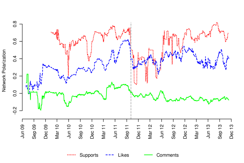
Figure 3: Time series of Q-modularity by party labels of the layers of supports (red), likes (blue) and comments (green). The grey dashed line denotes Swiss federal parliament election in 2011. Two trends can be observed: polarization among politicians peaks at pre-election time in the network of likes, and post-election time is characterized by lower levels of polarization in likes and comments.

Figure 3 shows the time series of network polarization along party lines for the three layers of the network. The comments layer shows negligible levels of polarization, fluctuating around $0$ for the whole time period. Polarization in likes shows an increasing pattern up to late 2011, reaching a value above 0.6 shortly before the Swiss federal parliament election in 2011. Right after the election, polarization in likes strongly corrects to levels slightly above $0.2$. Similarly, polarization in supports has relatively stable values around $0.6$ before the federal election, dropping to values below $0.3$ right afterwards. This analysis shows that network polarization, as portrayed in the online activity of politicians, is not a stable property of a political system, revealing that politically relevant events bias politician behavior in two ways: polarization reaches maxima during campaign periods, and polarization levels relax quickly after elections.

The pattern in likes suggests that politicians avoid awarding a like to a politician of another party when elections are close, but in other periods they display a less polarized pattern that allows likes across parties. On the other hand, polarization in supports stays generally high in the whole period of analysis but after the election, which suggests that some election winners might concentrate support, lowering party polarization along coalition structures. The patterns of polarization changes become evident when comparing the amount of intra- and inter-party connections in different periods: In the months of September and October 2011 the polarization before the election manifests in 618 (54.4%) likes within parties and 518 (45.6%) likes across parties, in comparison to the low polarization period a year before, in September and October 2010, when there were 300 (33.7%) likes within parties and 591 (66.3%) likes across parties. These observations, while sensitive to the size and activity in the network, appear in contrast with the control scenario of comments, in which no artificial pattern of party polarization appears in the whole period.

5 Party structures

In this section, we focus in two aspects of online political activity that are not captured by polarization metrics, i.e. intra-party structures and inter- party connectivity. In particular, we want to answer two questions: Do parties with different ideologies create different social structures in online communities? And do parties with similar positions in political space connect more to each other, despite the general pattern of polarization?

5.1 Intra-party structures

Previous research on the online political activity of users in the US discovered that right-leaning users showed higher online social cohesion than left-leaning users (Conover et al., 2012). In the following, we extend the quantification of each party both in its social structure and position in ideological space. With respect to the latter, we locate the ideology of each party in the two-dimensional space of Left-Right and Conservative-Liberal dimensions. To ensure the statistical relevance of our metrics, we restrict our analysis to the 6 parties with more than $200$ politicians each, which cover the two- dimensional spectrum of Swiss politics.

We analyze the social structure of each party based on the supports subnetwork among the politicians of the party, capturing the asymmetric relationships that lead to prestige and popularity. On each of these party subnetworks, we quantify three metrics related to relevant properties of online social networks: hierarchical structures through in-degree centralization, information efficiency through average path length, and social resilience through maximum k-core numbers (see Appendix D). While these three metrics are not independent from each other, they capture three components of online political activity that potentially differentiate parties: how popular their leaders are in comparison to a more egalitarian structure, how efficient their social structure is for transmitting information, and how big is the core of densely connected politicians who would support each other under adverse conditions.

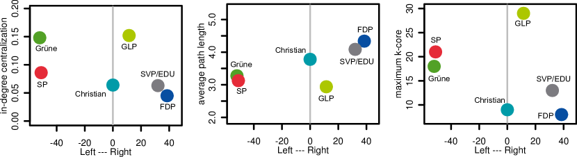
(a)

(b)

Figure 4: Social network metrics versus their position in ideological space, Left-Right position (top), Conservative-Liberal position (bottom). The supports subnetworks of parties with federal representation and more than 200 politicians each in politnetz.ch.

Figure 4 shows the value of the three social network metrics versus the position of each party in both dimensions. The two parties in the farthest right part of the spectrum, SVP and FDP, show higher average path lengths and lower maximum k-core numbers than left-wing parties such as SP and Grüne. This points to a difference in online activity in Switzerland dependent on the the political position of parties: right parties have created online social networks with lower information efficiency and lower social resilience. This poses a contrast with previous findings for US politics, in which politically aligned communities displayed the opposite pattern. This leads to the conclusion that the position of an online community in the left- right political spectrum does not universally define the properties of its social structure, and that particularities of each political system create different patterns.

There is no clear pattern of in-degree centralization in the Left-Right or Liberal-Conservative dimensions, but green parties (GLP and Grüne) show a significantly higher in-degree centralization than the rest. This result can be explained by the structure of the Swiss government, which is composed of seven politicians from a coalition of various parties. At the time of the study, this coalition includes politicians from the other four parties, excluding both GLP and Grüne. This would give an incentive to these parties to highlight a relevant member in order to gain a seat in the seven- member government, and thus creating higher in-degree centralization in online media.

5.2 Inter-party connectivity

Our second question tackles the activity across parties with respect to their political position, hypothesizing that parties closer in ideological space will be more likely to connect to each other. To do so, we first require a measure to estimate the tendency of one party to connect to another under the presence of polarization. To complement our analysis of Q-modularity, we use demodularity between pairs of parties, comparing their tendency to connect with what could be expected from a random network (see Appendix E). Negative demodularity indicates that a party consistently avoids interaction with another party, contrary to positive demodularity, which indicates that interactions are more frequent than expected at random.

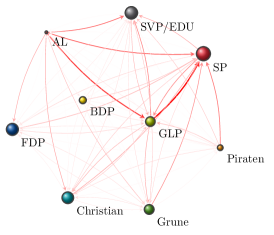
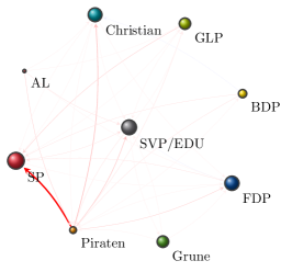
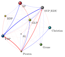
Figure 5: Networks of demodularity across parties for supports (left), likes (centre), and comments (right). Link width and color intensity is proportional to demodularity score between parties, colored blue for positive values and red for negative ones. Node size is proportional to the amount of politicians of each party. Demodularity scores are strongly negative for supports, weakly negative for likes, and both positive and negative for comments.

Figure 5 shows a visualization of the network of politicians aggregated by parties, for each layer of interaction. It can be observed that demodularity scores have strong negative values in the supports layer, where all links have a negative weight (more details in Appendix E). This is in line with the strong polarization among party lines, which makes support links to stay within parties. In addition, the overall level of outgoing negative demodularity shows a certain level of heterogeneity, as some parties have a stronger tendency to not support any politician from another party. In the likes layer, demodularity scores are less negative, indicating that there are weaker incentives to avoid giving a like to a politician of another party, compared to supports. Positive scores are only present in the comments layer, which shows that politicians are more likely to comment posts of other parties, creating debates with opponents.

To relate the demodularity with the position in ideological space of parties, we measured the Euclidean distance between pairs of parties in a two-dimensional ideological space, explained in detail in Appendix F. Our hypothesis is that in layers of interaction with positive connotation (supports and likes), parties that are further from each other have weaker cross-party interactions, in contrast to the comments layer, where links can be used to express disagreement and thus political distance increases with cross-party interaction. To test these hypotheses, we compute the Pearson correlation coefficient of the demodularity score of the pairs of parties versus the political Euclidean distance between them (see Appendix G for details). This correlation coefficient allows us to empirically test the existence of a linear relationship between ideological distance and cross-party interaction in each layer.

	Supports	Likes	Comments
$r_{\text{Pearson}}$	-0.14 ($p=0.37$)	-0.45 ($p<3\cdot 10^{-3}$)	0.45 ($p<2.7\cdot 10^{-3}$)

Table 6: Pearson correlation coefficients of the demodularity scores between parties and their pairwise Euclidean distance.

Table 6 shows the results for the three correlation coefficients. First, the supports layer shows no significant correlation, as data is not sufficient to reject the null hypothesis that both variables are not related. This points to the high level of polarization in supports, which makes links across parties so scarce that demodularity scores are equally negative for parties close and far in ideological space. The layer of likes shows a significant negative correlation, indicating that demodularity is higher between parties with closer ideologies. On the other hand, the correlation in the comments layer is positive, showing that politicians are more likely to participate in online debates with politicians of parties that hold opposite views. This highlights the meaning of comments, which are mainly used to argue with politicians of other parties as opposed to likes, which are used to agree with politicians with similar views, even though they might not belong to the same party.

6 Discussion

Our work explores behavioral aspects of political polarization, measuring network polarization over the digital traces left by politicians in politnetz.ch. Our approach is centered around the construction of a multiplex network with politicians as nodes and three layers of directed links: one with support links, a second one with link weights as the amount of comments a politician made to another politician, and a third one with weights counting the amount of times a politician liked the posts of another. We studied network polarization in the three layers as the level of intra-party cohesion with respect to inter-party cohesion, measuring network polarization as the modularity with respect to party labels, using Newman’s Q-modularity metric. This methodology allows us to investigate polarization at a scale and resolution not achievable by traditional opinion survey methods, including the time evolution of polarization on a daily basis. Furthermore, we provide a quantitative analysis of the ways in which politicians utilize participatory media, the content of discussion groups between politicians of different parties, and the conditions that increase and decrease online network polarization.

We compared the information shared across the three layers, and found that each layer contains a significant amount of link and community information that is not included in any other layer. The layers of supports and likes revealed significant patterns of polarization with respect to party alignment, unlike the comments layer, which has negligible polarization. This is particularly interesting with respect to opinion dynamics models, which frequently assume that the presence of opinion polarization implies a bias in the underlying communication network. While polarization is clearly present on politnetz with respect to like and support links, it does not seem to have decisive influence on overal communication. We applied community detection algorithms at all three layers, and compared the computationally found groups with the parties of the Swiss system. At the comments layer, the community detection algorithms reveal that a partitioning of politicians conveys higher modularity than party alignment, suggesting that groups in comments are not party-driven. This is confirmed by a content analysis of the comments in each group, where the most informative terms show that each group discusses different topics. At the supports layer, the partition of politicians into parties is very similar to the maximal partition found by algorithms, suggesting that party alignment is nearly the most polarizing partition of politicians. Further analysis will be necessary to test this observation, measuring how the party alignment of a politician might be predicted by its social context. In addition, our work focuses on data from politicians, constituting an analysis of elite polarization. Future works can include datasets from the electorate at large, measuring mass polarization from other digital traces such as blogs (Adamic and Glance, 2005) and Twitter (Conover et al., 2011).

We computed the time series of network polarization of each layer, revealing how the polarization in likes increased significantly around the federal elections of 2011, compared to moments without electoral campaigns. Polarization in supports and likes showed a sharp decrease after the elections, possibly as an effect of coalition-building processes, and polarization in comments was close to 0 for the whole study period. The evolution of polarization in likes and supports reveals a relation between online activity and political events, in which social interaction becomes more influenced by party membership when elections are close. Our approach to the time evolution of polarization can be applied to test the influence of other political events, for example how referendums might increase polarization along the opinions about the issue being voted.

The comments layer showed no party-alignment polarization, but the computational detection of modular structures reveals a different partition of politicians. Our analysis of the content of the comments in these partitions reveals that they follow different topics, and that modularity in comments can be attributed to similar interests and competences among politicians. This is emphasized when analyzing demodularity across parties and ideological distance: demodularity in comments increases with ideological distance, showing that parties that are further from each other tend to create debates in which politicians of different views comment on each other’s contributions. Furthermore, demodularity in likes decreases with distance between parties, showing that the missing polarization in likes is due to politicians acknowledging the contributions of people from other parties with similar ideologies. It keeps open to test the role of other possible aspects of the connectivity across parties, including geographical distribution, party size, and year of creation. Further analysis can test if new parties connect to other new parties across ideological distance and if their growths are correlated with connectivity, similarly to the growth of new European parties with information seeking (Bright and Yasseri, 2014). At the level of individual politicians, our methods allow the analysis of the relation between individual reputation and contribution to polarization, quantifying if strong biases in online behavior are tied to intra-party leadership and election results.

We analyzed the social networks of politicians in politnetz.ch to explore the relation between ideology and social structures in online interaction. We found that green parties (GLP and Grüne) have a higher in- degree centralization than the rest, indicating that their internal structure is more unequal with respect to popularity. Two possible explanations for this are the current configuration of the Swiss government, which excludes these two parties, or a hypothetical relation between environmental politics and party organization. Left-aligned parties have lower average path length and higher maximum k-core numbers than right-aligned ones, showing that left parties create social networks with higher information spreading capabilities than right parties. This result is in contrast with previous findings (Conover et al., 2012) which found the opposite pattern for the networks of US Twitter users. In addition, demodularity metrics across parties indicate that their connectivity in terms of likes increases with closeness in political space, while the connectivity in terms of comments increases with distance. These findings lead to a set of hypotheses to test in other multi-party systems, in order to understand the conditions that link online social network structures and the political position of parties. The digital traces left by politicians in Canada (Gruzd and Roy, 2014), Germany (Lietz et al., 2014), and Spain (Aragón et al., 2013) are first potential candidates for this kind of analyses.

Our results highlight that the strategies for campaigning and mobilization in online media differ with respect to the political position of a party, and that polarization in online behavior is heavily influenced by party membership and upcoming elections. Our findings show that the previously found relations between social network structures and ideology are not universal, calling for new theories that apply for multi-party systems. We showed that the analysis of network polarization through digital traces conveys an alternative approach to traditional survey methods, capturing elements of the time dependence and the phenomena that influence polarization. The multi-party nature of Switzerland and the crowdsourced online activity of its politicians allowed us to test the relation between the ideological distance and online interaction between parties, showing us a very clear picture of online interaction. First, supports are strongly biased towards politicians of the same party. Second, comments happen across parties of different political views, clustering politicians into groups with similar interests. And third, likes cross party lines towards politicians of similar opinions, but this effect is attenuated when elections are close, creating a highly polarized state that relaxes after elections are over.

7 Acknowledgements

This work was funded by the Swiss National Science Foundation (CR21I1_146499). We thank politnetz.ch for their support on the data retrieval.

Appendix A Appendix: Layer similarity metrics

A.1 Jaccard Similarity Coefficient

The Jaccard similarity coefficient is used to compare similarity and diversity between two sets. Its value for sets $X$ and $Y$ is defined as a division of the intersection of two sets over the union of these sets:

$$J_{XY}=\frac{|X\cap Y|}{|X\cup Y|}$$

For computing one-sided overlaps, the Partial Jaccard coefficient normalizes over one set only. For instance, the $J_{XY}$ normalized over $Y$ gives the fraction of the set $Y$ which is attributed to the set $X$:

$$\text{Partial }J_{XY}=\frac{|X\cap Y|}{|Y|}$$

A.2 Mutual information

Shannon’s Entropy

Claude Shannon introduced in 1948 the following measure of information through the entropy of the information source. Entropy stands for the measure of uncertainty of the information content, or how much of the uncertainty will be reduced when information is received. We illustrate a connection between the words information and entropy on the example of a coin toss.

A biased coin with both sides having heads will always land heads as a result of any toss event. If $X_{\text{biased}}$ is a random variable representing the result of a coin toss, then $p(X_{\text{biased}}=\text{Heads})=1$ and $p(X_{\text{biased}}=\text{Tails})=0$. Before the coin toss, our uncertainty about the result is negligible, since we know that at every trial the coin lands heads in anyway. We call that the entropy of such a process is small. Furthermore, after tossing the coin we can also state that we learn nothing new as outcome is known a priori, that is the amount of the uncertainty reduced is negligible, and thus the information received is also negligible. Assume that we toss an unbiased coin with equal probabilities of having heads or tails, $p(X_{\text{unbiased}}=\text{Heads})=\frac{1}{2}$ and $p(X_{\text{unbiased}}=\text{Tails})=\frac{1}{2}$. In this setup the uncertainty we have about the result of the event is the highest, since this coin can land heads or tails with equal probabilities. The entropy of this process is high, and thus the amount of the information received after each coin toss is also high.

If the result of a random variable is difficult to predict, then the entropy, unpredictability or uncertainty, of the outcome is high; conversely, if the result is predictable, it’s entropy is low. Entropy is at its highest value, when the outcomes of a random variable are equally probable. Shannon (1948) proved that only a logarithmic function satisfies the properties necessary to measure the entropy, and proposed the following formula:

$$H(A)=-\sum\limits_{i=1}^{m}p(a_{i})\cdot log_{b}p(a_{i})$$

where $A$ is a discrete random variable taking $m$ possible values $(a_{1},a_{2},\dots,a_{m})$, $p(a_{i})$ is the probability of $A$ taking value $a_{i}$, and $b$ is the base of the logarithm used which determines the information units of the entropy. For $b=2$, the entropy is measured in the number of bits per random variable outcome. Additionally, information can be expressed in terms of the entropy as:

$$I=k\cdot H(A)$$

where $k$ is the number of events. Therefore, with the logarithm of base $2$, information is measured in bits.

Thus, a coin that always falls heads has the entropy of $H(X_{\text{biased}})=-(0\cdot log_{2}0+1\cdot log_{2}1)=0$ bits per outcome which gives us no information after each throw, i.e. $I=1\cdot 0=0$ bits. On the other hand, the entropy of an unbiased coin is $H(X_{\text{unbiased}})=-(\frac{1}{2}\cdot log_{2}\frac{1}{2}+\frac{1}{2}\cdot log_{2}\frac{1}{2})=1$ bit per outcome, and the information received is $I=1\cdot 1=1$ bit.

Miller-Madow Entropy Estimator

Calculation of the entropy from the data samples requires the knowledge on the probabilities of the outcome of the random variable as seen from the Shannon’s formula. In practice, $p(a_{i})$ is unknown and must be estimated from the observed counts of the $i$-th outcome in the sequence of trials. The simplest and widely used estimator of the entropy is the Maximum Likelihood estimator (ML), (Hausser and Strimmer, 2009):

$$\hat{H}^{ML}(A) = -\sum\limits_{i=1}^{m}\hat{p}^{ML}(a_{i})\cdot log_{2}\hat{p}^{ML}(a_{i})$$

where $\hat{p}^{ML}(a_{i})$ is an estimate of the probability of the $i$-th possible outcome $a_{i}$ of the random variable, often calculated as $\hat{p}^{ML}(a_{i})=\frac{y_{i}}{n}$, where $y_{i}\geq 0$ is the number of the observed counts of the $i$-th outcome out of the $n$ number of observations.

When the number of the possible outcomes of the random variable is much lower than the number of observations, $m\ll n$, the ML method gives the optimal estimation of the entropy. On the other hand, the finite sample sizes can leave some outcomes unobserved, and the ML method can underestimate the true entropy. To overcome the sample size bias, corrections and other estimators of the entropy have been developed (Hausser and Strimmer, 2009). For our empirical estimation of the information content, we employ the Miller-Madow entropy estimator (Miller, 1955). In essence, it is the ML entropy with the bias correction:

$$\hat{H}^{MM}(A)=\hat{H}^{ML}(A)+\frac{p_{>0}-1}{2\cdot n}$$

where $p_{>0}$ is the number of outcomes with $y_{i}>0,\forall i\in[1..m]$, i.e. how many of the $m$ possible outcomes were observed in $n$ trials.

Mutual Information

If $X$ and $Y$ are two random variables, then the mutual information between them is expressed as:

$$I(X;Y)=H(X)-H(X|Y)=H(X)+H(Y)-H(X,Y)$$

where H(X), H(Y) are the marginal entropies, or simply the entropies of $X$ and $Y$; $H(X,Y)$ is the joint entropy of $X$ and $Y$, and $H(X|Y)$ is the conditional entropy of $X$ given $Y$, which is the amount of the uncertainty that remains in $X$ when the value of $Y$ is known. The mutual information measures the average reduction of the uncertainty in $X$ that results from learning $Y$; and vice versa (MacKay, 2002).

The mutual information is symmetric, $I(X;Y)=I(Y;X)$, and is depicted in relation to the entropy in Figure 6.

H(X,Y)
H(X)
			H(Y)
H(X|Y)			I(X;Y)		H(Y|X)

Figure 6: The relationship between the joint entropy, the marginal entropy, the conditional entropy and the mutual information (MacKay, 2002).

The mutual information can be measured in terms of the probabilities of the outcomes of the random variables:

$$I(X;Y)=\sum\limits_{y\in Y}\sum\limits_{x\in X}p(x,y)\cdot log_{2}\left(\frac{p(x,y)}{p(x)\cdot p(y)}\right)$$

where $p(x,y)$ is the joint probability distribution of $X$ and $Y$, and $p(x)$ and $p(y)$ are the marginal probabilities of the outcomes $x$ and $y$. We compute the entropy and the mutual information using the Entropy library of the R programming language developed by Hausser and Strimmer (2009).

Normalized Mutual Information

This metric is also known as the uncertainty coefficient, (Press et al., 2007). The uncertainty coefficient of $X$ with respect to $Y$ is given by:

$$\text{NMI}(X|Y)=\frac{I(X;Y)}{H(X)}=\frac{H(X)-H(X|Y)}{H(X)}$$

In essence, the uncertainty coefficient of the dependent variable $X$ with respect to the independent variable $Y$ is the mutual information of both variables normalized over the entropy of the dependent variable. The measure lies between $0$ and $1$, and is interpreted as follows: if the NMI$(X|Y)=0$, then there is no relation between $X$ and $Y$; if the NMI$(X|Y)=1$, then the knowledge of $Y$ fully predicts or determines $X$, or 100% of the information content of $X$ is captured by $Y$. A value in-between $0$ and $1$ gives the fraction of the information gain of $X$ when $Y$ is known. Interchanging $X$ and $Y$ in the uncertainty coefficient, NMI$(Y|X)$, will define the dependence of $Y$ with respect to $X$, and the normalization is performed over the entropy of $Y$.

Appendix B Appendix: Measuring network polarization

B.1 Q-modularity

In the network theory, a network shows a modular structure if it can be partitioned into the groups that are densely interconnected inside and loosely connected to the other groups. The Q-modularity metric quantifies the quality of a partition in terms of a modular structure (Newman, 2006), comparing the fraction of links of nodes within the groups to the expected value if links were distributed purely at random, but preserving the nodes’ degrees. The formula for a directed network is given by:

$$Q=\frac{1}{m}\cdot\sum\limits_{i=1}^{N}\sum\limits_{j=1}^{N}\left[A_{ij}-\frac{k_{i}^{\text{out}}\cdot k_{j}^{\text{in}}}{m}\right]\delta(i,j)$$

where $N$ and $m$ are the amounts of nodes and links in the network, $k_{i}^{\text{out}}$ and $k_{i}^{\text{in}}$ are the out-degree and the in-degree of node $i$, $A$ is the adjacency matrix of the network, and $\delta(i,j)$ is a function that takes the value 1 if nodes $i$ and $j$ are in the same group, and $0$ otherwise. For the case of a weighted network, the amount of links is replaced with the sum of weights of all links, and the adjacency matrix has entries corresponding to the weight of each link.

B.2 Community detection algorithms

In an arbitrary network, finding a partition with the maximum Q-modularity is known as the community detection problem. There is a wide variety of algorithms producing different network partitions which aim at finding a partition with the maximum Q-modularity. To find partitions with the maximal modularity in each layer, we used the state-of-the-art community detection algorithms from the open source software Radatools, (Gómez, 2011). Following is the list of the algorithms that are implemented in the software, abbreviations of the algorithms are given in brackets:

• (e): extremal optimization, see (Duch and Arenas, 2005)

• (s): spectral optimization, see (Newman, 2006)

• (f): fast algorithm, see (Newman, 2003)

• (r): fine-tuning by reposition

The algorithms (s) and (e) have a stochastic behaviour, thus they must be executed with several repetitions, e.g. (esrfr-30) means perform 30 repetitions of the algorithm (e), 30 repetitions of (s), 1 times (r), 1 times (f) and finally 1 times (r), refer to the (Gómez, 2011) for more details. We run the following combinations of the algorithms for each layer: e-1, esrfr-30, r-1, f-1, s-10, rfr-1, rsrfr-30, and store the partition that gives the highest Q-modularity from among all the runs. This optimal partition, which is computed independently from the party alignment, determines the $Q_{comp}$ polarization score. We repeated this analysis for each layer, which resulted in three values of the $Q_{comp}$: one for supports, one for likes, and another one for comments.

B.3 Time series of network polarization

We construct a time series of polarization with a rolling window technique, dividing the network data along the time axis in the overlapping intervals of a fixed size. Each interval overlaps with the next one on a fixed subinterval, where the difference in their starting dates is a constant step size. This technique smooths out the data through the aggregation of links within the window, and preserves a granularity defined by the step size. For our analysis, we chose a window of 2 months and a 1-day step, in order to aggregate sufficient data in each window and to preserve daily resolution in the time series. In every time interval, we compute the Q-modularity on the network with links that have timestamps within the specified interval. We illustrate the method with an example and Figure 7. At the timestamp of the first link, $t$, we obtain the first- window modularity score for the interval $[t,t+\text{2 months}]$, then we move the window one step forward to the starting time $t^{\prime}=t+\text{1 day}$, recompute the metric on the network with the links present within the new window, to obtain the modularity score at the time $t^{\prime}$. We continue sliding the time window, computing the modularity until reaching the timestamp of the last link. Hence, with this approach, we record the evolution of the network polarization around the dates in each time window.

$\cdots$	$w$ = 2 months, $Q^{t}$			$\cdots\cdots\cdots\cdots\cdots\cdots\cdot$
$\cdots$	1 day	$w$ = 2 months, $Q^{t^{\prime}}$			$\cdots\cdots\cdots\cdot\cdot$
$\cdots\cdots\cdots\cdot\cdot$		1 day	$w$ = 2 months, $Q^{t^{\prime\prime}}$			$\cdots$

Figure 7: Time-series segmentation approach of computing modularity score of a network with a sliding window. At each shift of the window, modularity is computed on the network with the links present within the current time window. The size of the window is set at 2 months, the step of the window shift is 1 day.

Appendix C Appendix: Word information content

Pointwise Mutual Information

The PMI is the mutual information for the pairs of outcomes of two random variables rather than all possible values. Thus, there is a direct link between the MI and the PMI: the mutual information of the two random variables $X$ and $Y$ is the expected value of the PMI over all possible pairs of outcomes of the two random variables.

$$\text{PMI}(X=x;Y=y)=log_{2}\frac{p(x,y)}{p(x)\cdot p(y)}=log_{2}\frac{p(x|y)}{p(x)}=log_{2}\frac{p(y|x)}{p(y)}$$

where $p(x,y)$ is the joint probability distribution of the outcomes $x$ and $y$ of the random variables $X$ and $Y$ respectively, and $p(x)$ and $p(y)$ are the marginal probability distributions of the outcomes $x$ and $y$ of the random variables $X$ and $Y$ respectively.

We use the PMI to detect the information that a word contains within a set of comments in a group of the comments layer, approximating $p(x)$ as the total frequency of the word in all comments, and $p(x|y)$ as the frequency of the word within the comments of the group. To control for statistical significance, we performed $\chi^{2}$ tests on the ratio of frequencies, filtering out words with the PMI significance below the 99% confidence level. This gives us a list of words with significantly high PMI for each comment group, indicating the most informative terms of the discussions within each group of politicians.

Appendix D Appendix: Intra-party social network metrics

D.1 In-degree Centralization

Freeman (1979) introduced the concept of degree centralization, where the average difference between the node degree centralities is normalized over the value for a star network. In our case, we use this idea to capture hierarchical structure inside the parties through the in-degree centralization:

$$C_{in}=\frac{\sum\limits_{i=1}^{n}\left[k^{in}_{*}-k^{in}_{i}\right]}{\text{max}\sum\limits_{i=1}^{n}\left[k^{in}_{*}-k^{in}_{i}\right]}$$

where $k^{in}_{i}$ is the in-degree of node $i$, $k^{in}_{*}$ is the largest in-degree of the network and ${\text{max}\sum\limits_{i=1}^{n}\left[k^{in}_{*}-k^{in}_{i}\right]}$ is the maximum possible sum of differences in the degree centrality, which corresponds to the value of a star network.

The numerator represents the sum of differences between the highest degree in the graph given by node $v*$ and the degrees of the other nodes, measuring the extent to which the most central node $v*$ exceeds the in-degree of the other nodes. The denominator stands for the maximum possible value of such difference in the network with the same number of nodes. (Freeman, 1979) showed that the maximum difference is achieved in the networks of a star-like structure where one node dominates the network with respect to its centrality, and produces the degree centrality of the highest value of $1$; conversely, the lowest boundary of $0$ is obtained in complete networks, e.g. cliques, where all possible links between nodes are present, and thus, nodes are homogeneous and equal. Normalized over the denominator, the degree centrality is a value in the interval $[0,1]$ and represents the average deviation of nodes in the network from the most central node.

D.2 Average Path Length

This social network metric measures the efficiency of the information transportation in a network:

$$l(G)=\frac{1}{n\cdot(n-1)}\cdot\sum\limits_{i=1}^{n}\sum\limits_{j=1}^{n}d(v_{i},v_{j}),\forall i\neq j$$

where $d(v_{i},v_{j})$ is the length of the shortest path between nodes $v_{i}$ and $v_{j}$, and $n$ is the number of nodes in the network. In essence, the average path length is the sum of the lengths of the shortest paths between all pairs of nodes in the network divided over the maximum number of all possible pairs, $\forall i,j$ s.t. $i\neq j$, in the network where a path can exist, therefore the normaliztion factor is $\frac{1}{n\cdot(n-1)}$. If the network consists of the disconnected components, the normalization factor becomes the number of existing paths in the network:

$$l(G)=\frac{1}{\sum\limits_{i=1}^{n}\sum\limits_{j=1}^{n}\delta(i,j)}\cdot\sum\limits_{i=1}^{n}\sum\limits_{j=1}^{n}d(v_{i},v_{j}),\forall i\neq j$$

where $\delta(i,j)=1$ if there exists a path between the nodes $i$ and $j$, $0$ – otherwise.

D.3 k-core Decomposition

A $k$-core of a network is a sub-network in which all nodes have a degree $\geq k$. The $k$-core decomposition is a procedure of finding all $k$-cores, $\forall k>0$, by repeatedly pruning nodes with degrees $k$. Therefore, it captures not only the direct, but also the indirect impact of users leaving the network. As an illustration consider Figure 8, which shows the process of finding the $k$-core decomposition:

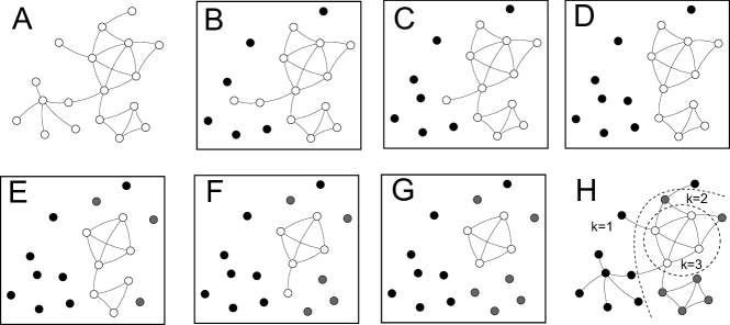
Figure 8: Effects of node removals on network connectivity as captured by degree only (A $\rightarrow$ B) and $k$-core decomposition (A $\rightarrow$ C $\rightarrow$ D $\rightarrow$ E)

Starting again from A, and applying the $k$-core procedure, will repeatedly remove nodes of degree less than 2, until only those with degree of at least 2 remain in panel D. The removed nodes up to this point are in the 1-core of the network but not in the 2-core. In a second iteration, all nodes of degree less than 3 are removed, colored dark gray in panel G. These form part of the 2-core of the network, but not of the 3-core, which is composed of the last four nodes. Hence, supposing that users leave a community when they are left with less than 3 friends, the $k$-core decomposition captures the full cascading effect that departing users have on the network as a whole. More details on the empirical calculation of the k-core decomposition can be found elsewhere (Garcia et al., 2013).

Appendix E Appendix: Demodularity

We introduce an inter-group measure called demodularity, which quantifies the relationship across different groups rather than within the group, and can be defined as a property of a network where nodes of one group preferentially attach to the nodes of the other group. Negative scores of the demodularity from group $f$ to group $t$ indicate that nodes of $f$ strongly avoid interactions with nodes of $t$, contrary to positive scores that show cross- community interactions. The demodularity, $\overline{Q}_{ft}$, from community $f$ to community $t$ in a directed network is defined as:

$$\overline{Q}_{ft}=\frac{1}{m_{f}}\cdot\sum\limits_{i=1}^{N}\sum\limits_{j=1}^{N}\left[A_{ij}-\frac{k_{i}^{\text{out}}\cdot k_{j}^{\text{in}}}{m}\right]\delta(C(i),f)\cdot\delta(C(j),t)$$

where $C(i)$ is the group to which node $i$ belongs, $\delta(C(i),f)$ is a function such that $\delta(C(i),f)=1$ if the group of node $i$ is $f$, and $0$ otherwise, and the rest of the notation is consistent with the definition of Q-modularity of Appendix B.1.

Tables 7, 8, 9 show the demodularity scores for the layers of supports, likes and comments.

	AL	BDP	Christian	FDP	GLP	Grune	Piraten	SP	SVP/EDU
AL	-	-0.012	-0.046	-0.043	-0.099	-0.036	-0.016	-0.077	-0.07
BDP	-0.002	-	-0.01	-0.006	-0.021	-0.014	-0.004	-0.034	-0.016
Christian	-0.002	-0.003	-	-0.012	-0.031	-0.014	-0.006	-0.046	-0.021
FDP	-0.002	-0.003	-0.013	-	-0.028	-0.016	-0.005	-0.042	-0.014
GLP	-0.005	-0.009	-0.039	-0.033	-	-0.045	-0.011	-0.125	-0.06
Grune	-0.003	-0.005	-0.019	-0.02	-0.044	-	-0.008	-0.055	-0.032
Piraten	-0.002	-0.005	-0.023	-0.019	-0.039	-0.024	-	-0.066	-0.031
SP	-0.003	-0.007	-0.03	-0.027	-0.058	-0.024	-0.01	-	-0.043
SVP/EDU	-0.003	-0.003	-0.015	-0.01	-0.038	-0.022	-0.007	-0.057	-

Table 7: The demodularity scores of the layer of supports. Scores in the range $(-0.1,-0.05]$ are highlighted in light red colour, and scores in the range $(-\infty,-0.1]$ are displayed in red.

	AL	BDP	Christian	FDP	GLP	Grune	Piraten	SP	SVP/EDU
AL	-	0	-0.001	-0.001	-0.001	0	-0.003	0	-0.002
BDP	0	-	0.001	0	0	0	-0.002	-0.002	0
Christian	0	0	-	-0.001	0	0	-0.001	-0.001	-0.001
FDP	0	0	0	-	0	0	-0.001	-0.002	0
GLP	0	0	0	-0.001	-	0	0	-0.003	-0.001
Grune	0	0	0	-0.001	0	-	-0.001	0	-0.001
Piraten	0	-0.001	-0.005	-0.003	-0.002	-0.003	-	-0.016	-0.004
SP	0	0	-0.001	-0.001	-0.001	0	-0.003	-	-0.002
SVP/EDU	0	0	0	0.001	-0.001	-0.001	-0.002	-0.003	-

Table 8: The demodularity scores of the layer of likes.

	AL	BDP	Christian	FDP	GLP	Grune	Piraten	SP	SVP/EDU
AL	-	0	0	0	-0.001	-0.001	0.002	-0.001	-0.002
BDP	0	-	-0.001	-0.003	0.002	0.001	-0.001	0.002	-0.001
Christian	0	0	-	-0.001	0	0	0.001	-0.001	-0.002
FDP	0	0	-0.002	-	-0.002	0	-0.002	0.005	0.002
GLP	0	-0.001	0	-0.005	-	0	0.002	-0.004	0.004
Grune	0	0	0	-0.001	0	-	0	-0.001	0.002
Piraten	0	-0.001	0.004	-0.007	0.005	-0.003	-	0	-0.006
SP	0	0	-0.001	0.001	-0.001	-0.001	0	-	0.003
SVP/EDU	0	0.001	0	0.007	0	0.002	-0.003	0	-

Table 9: The demodularity scores of the layer of comments. Positive scores in the range $(0,0.005)$ are highlighted in light blue colour, and scores in the range $[0.005,\infty)$ are displayed in blue.

Appendix F Appendix: Political distance

The Euclidean distance between two points $\mathbf{X}$ and $\mathbf{Y}$ is the length of the line segment connecting them: $\mathbf{\overline{XY}}$. In Cartesian coordinates, if $\mathbf{X}=(x_{1},x_{2},\dots,x_{n})$ and $\mathbf{Y}=(y_{1},y_{2},\dots,y_{n})$ are two points in the Euclidean $n$-space, then the distance between $\mathbf{X}$ and $\mathbf{Y}$ is defined as:

$$\mathbf{d}(\mathbf{X},\mathbf{Y})=\sqrt{(x_{1}-y_{1})^{2}+(x_{2}-y_{2})^{2}+\dots+(x_{n}-y_{n})^{2}}$$

Each of the parties $\mathbf{X}$ and $\mathbf{Y}$ has two political position coordinates: Left-Right (lr) and Liberal-Conservative (lc). If $\mathbf{X}=(x_{lr},x_{lc})$ and $\mathbf{Y}=(y_{lr},y_{lc})$, then the Euclidean party distance is given by:

$$\mathbf{d}(\mathbf{X},\mathbf{Y})=\sqrt{(x_{lr}-y_{lr})^{2}+(x_{lc}-y_{lc})^{2}}$$

Appendix G Appendix: Correlation estimation

The Pearson correlation coefficient is a measure of the association between two variables $X$ and $Y$, and is defined as the covariance of the two variables divided by the product of their standard deviation:

$$r=\frac{\sum\limits_{i=1}^{n}(x_{i}-\overline{X})\cdot(y_{i}-\overline{Y})}{\sqrt{\sum\limits_{i=1}^{n}(x_{i}-\overline{X})^{2}}\cdot\sqrt{\sum\limits_{i=1}^{n}(y_{i}-\overline{Y})^{2}}}$$

where $\overline{X}$ and $\overline{Y}$ are the mean of each of the random variables, and $x_{i}$, $y_{i}$ are the $i$-th outcome of the random variables $X$ and $Y$ respectively.

References

- Adamic and Glance (2005) Adamic, L. A.; Glance, N. (2005). The Political Blogosphere and the 2004 U.S. Election: Divided They Blog. In: Proceedings of the 3rd International Workshop on Link Discovery. LinkKDD ’05, New York, NY, USA: ACM, pp. 36–43.
- Aragón et al. (2013) Aragón, P.; Kappler, K. E.; Kaltenbrunner, A.; Laniado, D.; Volkovich, Y. (2013). Communication dynamics in twitter during political campaigns: The case of the 2011 Spanish national election. Policy & Internet 5(2), 183–206.
- Baldassarri and Bearman (2007) Baldassarri, D.; Bearman, P. (2007). Dynamics of political polarization. American sociological review 72(5), 784–811.
- Blau (1977) Blau, P. M. (1977). Inequality and heterogeneity: A primitive theory of social structure, vol. 7. Free Press New York.
- Boccaletti et al. (2014) Boccaletti, S.; Bianconi, G.; Criado, R.; Del Genio, C.; Gómez-Gardeñes, J.; Romance, M.; Sendina-Nadal, I.; Wang, Z.; Zanin, M. (2014). The structure and dynamics of multilayer networks. Physics Reports 544(1), 1–122.
- Bright and Yasseri (2014) Bright, J.; Yasseri, T. (2014). Electoral Politics and Information Seeking on the Social Web: Towards Theoretically Informed Big Data Analytics. In: The Internet, Policy & Politics Conference. Unpublished.
- Cardillo et al. (2013) Cardillo, A.; Gómez-Gardeñes, J.; Zanin, M.; Romance, M.; Papo, D.; Del Pozo, F.; Boccaletti, S. (2013). Emergence of network features from multiplexity. Scientific reports 3.
- Conover et al. (2011) Conover, M.; Ratkiewicz, J.; Francisco, M.; Gonçalves, B.; Menczer, F.; Flammini, A. (2011). Political polarization on twitter. In: International AAAI Conference on Weblogs and Social Media.
- Conover et al. (2012) Conover, M. D.; Gonçalves, B.; Flammini, A.; Menczer, F. (2012). Partisan asymmetries in online political activity. EPJ Data Science 1(1), 1–19.
- Duch and Arenas (2005) Duch, J.; Arenas, A. (2005). Community detection in complex networks using extremal optimization. Phys Rev E 72(027104).
- Fiorina and Abrams (2008) Fiorina, M. P.; Abrams, S. J. (2008). Political polarization in the American public. Annu. Rev. Polit. Sci. 11, 563–588.
- Flache and Macy (2011) Flache, A.; Macy, M. W. (2011). Small worlds and cultural polarization. The Journal of Mathematical Sociology 35(1-3), 146–176.
- Freeman (1979) Freeman, L. C. (1979). Centrality in social networks conceptual clarification. Social networks 1(3), 215–239.
- Fruchterman and Reingold (1991) Fruchterman, T. M. J.; Reingold, E. M. (1991). Graph drawing by force-directed placement. Software: Practice and Experience 21(11), 1129–1164.
- Garcia et al. (2013) Garcia, D.; Mavrodiev, P.; Schweitzer, F. (2013). Social resilience in online communities: The autopsy of friendster. In: Proceedings of the first ACM conference on Online social networks. ACM, pp. 39–50.
- Garcia et al. (2012) Garcia, D.; Mendez, F.; Serdült, U.; Schweitzer, F. (2012). Political polarization and popularity in online participatory media: an integrated approach. In: Proceedings of the first edition workshop on Politics, elections and data. pp. 3–10.
- Germann et al. (2014) Germann, M.; Mendez, F.; Wheatley, J.; Serdült, U. (2014). Spatial maps in voting advice applications: The case for dynamic scale validation. Acta Politica .
- Gómez (2011) Gómez, S. (2011). Radatools software, Communities detection in complex networks and other tools. http://deim.urv.cat/~sgomez/radatools.php. [Online; accessed 27-October-2013].
- Groeber et al. (2009) Groeber, P.; Schweitzer, F.; Press, K. (2009). How groups can foster consensus: The case of local cultures. Journal of Aritifical Societies and Social Simulation 12(2), 1–22.
- Gruzd and Roy (2014) Gruzd, A.; Roy, J. (2014). Investigating political polarization on twitter: A canadian perspective. Policy & Internet 6(1), 28–45.
- Guerra et al. (2013) Guerra, P. H. C.; Meira Jr, W.; Cardie, C.; Kleinberg, R. (2013). A Measure of Polarization on Social Media Networks Based on Community Boundaries. In: International AAAI Conference on Weblogs and Social Media.
- Hausser and Strimmer (2009) Hausser, J.; Strimmer, K. (2009). Entropy Inference and the James-Stein Estimator, with Application to Nonlinear Gene Association Networks. J. Mach. Learn. Res. 10, 1469–1484.
- Hermann and Städler (2014) Hermann, M.; Städler, I. (2014). Wie sich die SVP aus dem Bürgerblock verabschiedet hat. WWW page.
- Hetherington (2009) Hetherington, M. J. (2009). Review article: Putting polarization in perspective. British Journal of Political Science 39(02), 413–448.
- Lietz et al. (2014) Lietz, H.; Wagner, C.; Bleier, A.; Strohmaier, M. (2014). When politicians talk: Assessing online conversational practices of political parties on twitter. In: International AAAI Conference on Weblogs and Social Media.
- MacKay (2002) MacKay, D. J. C. (2002). Information Theory, Inference & Learning Algorithms. New York, NY, USA: Cambridge University Press.
- McCarty et al. (2006) McCarty, N.; Poole, K. T.; Rosenthal, H. (2006). Polarized America: The dance of ideology and unequal riches, vol. 5. mit Press.
- Menichetti et al. (2014) Menichetti, G.; Remondini, D.; Panzarasa, P.; Mondragón, R. J.; Bianconi, G. (2014). Weighted multiplex networks. PloS one 9(6), e97857.
- Miller (1955) Miller, G. A. (1955). Note on the bias of information estimates. Information Theory in Psychology: Problems and Methods , 95–100.
- Newman (2003) Newman, M. (2003). Fast algorithm for detecting community structure in networks. Physical Review E 69.
- Newman (2006) Newman, M. E. (2006). Modularity and community structure in networks. Proc Natl Acad Sci U S A 103(23), 8577–8582.
- Press et al. (2007) Press, W. H.; Teukolsky, S. A.; Vetterling, W. T.; Flannery, B. P. (2007). Numerical Recipes 3rd Edition: The Art of Scientific Computing. New York, NY, USA: Cambridge University Press, 3 edn.
- Saunders and Abramowitz (2004) Saunders, K. L.; Abramowitz, A. I. (2004). Ideological realignment and active partisans in the American electorate. American Politics Research 32(3), 285–309.
- Schweitzer and Behera (2009) Schweitzer, F.; Behera, L. (2009). Nonlinear voter models: the transition from invasion to coexistence. The European Physical Journal B 67(3), 301–318.
- Seidman (1983) Seidman, S. B. (1983). Network structure and minimum degree. Social Networks 5(3), 269 – 287.
- Serdült (2014) Serdült, U. (2014). Referendums in Switzerland. In: M. Qvortrup (ed.), Referendums Around the World: The Continued Growth of Direct Democracy, Basingstoke: Palgrave Macmillan. pp. 65–121.
- Shannon (1948) Shannon, C. (1948). A Mathematical Theory of Communication. Bell System Technical Journal 27, 379–423, 623–656.
- Sunstein (2003) Sunstein, C. R. (2003). Why societies need dissent. Harvard University Press.
- Szell et al. (2010) Szell, M.; Lambiotte, R.; Thurner, S. (2010). Multirelational organization of large-scale social networks in an online world. Proceedings of the National Academy of Sciences 107(31), 13636–13641.
- Tufekci (2014) Tufekci, Z. (2014). Big Questions for Social Media Big Data: Representativeness, Validity and Other Methodological Pitfalls. In: International AAAI Conference on Weblogs and Social Media.
- Waugh et al. (2009) Waugh, A. S.; Pei, L.; Fowler, J. H.; Mucha, P. J.; Porter, M. A. (2009). Party polarization in congress: A network science approach. arXiv preprint arXiv:0907.3509 .