We know that our Universe is composed of only $\sim$ 4.5% “known” matter; therefore, our understanding is incomplete. This can be seen directly in the case of neutrino oscillations (without even considering potential other universes). Charm quarks have had considerable impact on our understanding of known matter, and quantum chromodynamics (QCD) is the only local quantum field theory to describe strong forces. It is possible to learn novel lessons concerning strong dynamics by measuring rates around the thresholds of $[\bar{Q}Q]$ states with $Q=b,c$. Furthermore, these states provide us with gateways towards new dynamics (ND), where we must transition from “accuracy” to “precision” eras. Finally, we can make connections with $\tau$ transitions and, perhaps, with dark matter. Charm dynamics acts as a bridge between the worlds of light- and heavy-flavor hadrons (namely, beauty hadrons), and finding regional asymmetries in many-body final states may prove to be a “game changer”. There are several different approaches to achieving these goals: for example, experiments such as the Super Tau-Charm Factory, Super Beauty Factory, and the Super $Z^{0}$ Factory act as gatekeepers – and deeper thinking regarding symmetries.

Keywords; CKM matrix, HQE & OPE, CPV in $\Delta C\neq 0\neq\Delta B$ & $\tau$ decays

PACS numbers: 11.30.Er, 12.15.Hh, 12.38.Aw, 13.25.Ft, 13.35.Dx

 

 

1 Landscapes for fundamental dynamics

At the end of the previous millennium, we realized that the Universe consists of greater variety than previously believed: known matter $\sim$ 4.5%, dark matter $\sim$ 26.5%, and vacuum (or dark) energy $\sim$ 69%. Since the beginning of this millennium, we have had the following knowledge regarding known matter:

(a) We have failed to understand the extremely large asymmetry between known matter and anti-matter in our Universe.

(b) The Standard Model (SM) produces the leading source of the measured charge parity (CP) violations in neutral kaons and $B$ transitions at least (except, possibly, in $B_{s}$ oscillations).

(c) No CP asymmetry has yet been established in charm hadron or baryon decays in general (apart from human existence).

(d) The neutral Higgs-like state has been found in the SM predicted mass region, and no sign of new dynamics (ND) has been observed in its decays as of yet. However, we know that the Higgs’ amplitude is primarily a scalar.

(e) It is possible that the impact of Dark Matter may be observed, in particular in CP asymmetries in charm hadrons decays. Furthermore, $\tau$ lepton decays may be used to calibrate those correlations. At minimum, we will learn novel lessons about non-perturbative QCD.

We know that the SM cannot produce neutrino oscillations; this was found with $\Delta m(\nu_{i})\neq 0$ & three non-zero angles. There is a reasonable chance of finding CP asymmetries in that case, despite the background nuclei and anti-nuclei asymmetries. Note that the definition of known matter is “fuzzy” or “subtle”.

In this review, I primarily focus on measured or measurable charm hadron transitions, but I do not ignore other phenomena and the information they can provide. Even when we cannot establish the existence of ND in these transitions, we learn novel lessons about the connections between strong & weak forces and the dynamics of beauty hadrons. In other words, the fundamental dynamics around thresholds of $\bar{H}_{c}H_{c}$ & $\tau^{+}\tau^{-}$ are complex and also provide indirect information about $H_{b}$ transitions, where $H_{c}$ and $H_{b}$ are heavy mesons containing a heavy ($c$ and $b$) and a light quark.

First, I will “paint” a picture of the flavor dynamics landscape. Charm quarks have changed the understanding of fundamental dynamics in several ways.

• Previously, quarks were primarily seen as a mathematical trick to describe the strong forces between hadrons. Not all researchers agreed with this concept, however. The charm quark was introduced for a simple reason, i.e., to describe connections between two quark and lepton families [1]. In 1970, it was suggested as a means of solving the subtle problem of flavor-changing neutral currents without tree diagrams [2]. The “Glashow-Iliopoulos-Maiani (GIM)” researchers gave the name “charm”, meaning to have “magic powers” to prevent bad luck – like charming a venomous snake cobra.

• A very good candidate event for the decay of a charm hadron was found by a group led by Niu in 1971, in emulsion exposed to cosmic rays and analyzed at Nagoya University [3]. $X^{\pm}\to h^{\pm}\pi^{0}$ was found, with $h^{\pm}$ denoting a charged hadron that can be a meson or baryons. With a lifetime of a few $10^{-14}$ s, this is a weak decay; if $h^{\pm}$ is a meson, the mass of $X^{\pm}$ is approximately 1.8 GeV. Actually, quarks were already seen as physical states by the physics department at Nagoya University; elsewhere, this concept was mostly ignored.

• In fact, it had already been pointed out in 1963 in the Russian version of Okun’s book [4], which was published before the discovery of CP violation (CPV), that charm hadrons could be found in multi-lepton events in neutrino production. Evidence for their existence was found by interpreting opposite-sign dimuon events: $\nu N\to\mu^{-}D...\to\mu^{-}\mu^{+}...$ [5].

• In a seminal 1973 paper, Gaillard and Lee [6] explored in detail how charm quarks affect $K^{0}-\bar{K}^{0}$ oscillations, $K_{L}\to\mu^{+}\mu^{-}/2\gamma$ through quantum corrections; their findings yielded a bound of $m_{c}\leq 2$ GeV. Together with Rosner, they extended this analysis in a review that was published in the summer of 1974 [7]. At the same time, it was suggested that charm and anti-charm quarks form an unusually narrow vector meson bound-state, as a result of gluons carrying three colors and their couplings decreasing with increasing mass scales [8]. Thus, the theoretical tools were in place to interpret the surprising observations that were to come. However, these reports did not convince the skeptics; they required a Damascus experience to change from “Saulus” into “Paulus”, i.e., from disbelievers into believers.

• Evidence was provided when an unusually narrow resonance in $e^{+}e^{-}$ collisions was detected at Stanford Linear Accelerator Center (SLAC) on the west coast of the US and $p\,Be$ collisions at Brookhaven National Laboratory (BNL) on the east coast in 1974. This narrow resonance produced an important “paradigm” shift, specifically, $J/\psi(1S)$ was seen as a boundstate $[\bar{c}c]$ (after passionate discussions for a year). This was also established by $\psi(2S)$ and $\psi(3.77)$; the latter produces a $D^{0}\bar{D}^{0}$ and $D^{+}D^{-}$ factory. As previously stated, I refer to this event as the “October revolution of 1974” in fundamental dynamics.

• Quarks are real physical states, but they can only be observed in boundstates, and are not free as named due to “confinement”. For several reasons, it was realized that unbroken local color $SU(3)_{C}$ describes “strong” forces from long to short distances.

• First, it was thought that two pairs of SM quarks were required, namely, up- & down-type quarks with $(u,c)$ & $(d,s)$ with charged $+2/3$ & $-1/3$, respectively, named $s=$“strange” & $c=$“charm”.

• On the other hand, the situation at that energy scale was and (& still is) considerably more complex, as mentioned above. After many more discussions & more careful analyses, researchers realized that the third lepton family with the charged $\tau$ had already been found. This also suggested that a third quark family existed, it “simply” had to be found.

• The Proceedings of the CCAST Symposium were produced by the Institute of High Energy Physics (Beijing) in 1987 [10]. I may appear to be biased in this regard; however, the Proceedings remain useful, and not only as regards the history of the field. We have made sizable progress in the past 27 years, but not in every respect, and careful readers of these Proceedings still find directions (or at least signposts) for future progress.

• Wolfenstein introduced the super-weak scenario in 1964 [11]. This scenario defined the CPV classes, but it is not a theory. In retrospect, this means that theorists were slow to deal with that challenge. Kobayashi & Maskawa published a paper in 1973 [12] that discussed the general landscape of CP asymmetries. From the beginning of the 21st century, we knew that the SM produces the leading source of the measured CPV at least, with three quark families (or more). Researchers obtained six triangles with different shapes, but with the same areas.

The book “A cicerone for the physics of charm” [13] relates the history of high-energy physics regarding flavor dynamics, and also significantly more: it indicates directions for future research. I will refer to it several times to aid readers; furthermore, very interested readers can see peruse the list of references (such as pioneering papers by Shifman & Voloshin [14]). Charm hadrons are primarily seen as somewhat heavy-flavor particles. Charm hadrons act as the bridge between the worlds of the light- and heavy-flavor hadrons. This means that the flavor depends on various factors. Often, it helps to understand both strong & weak dynamics. The research status regarding these topics has changed, as we currently have significantly more data along with superior analysis tools; furthermore, theoretical tools have evolved with more focus on accuracy & correlations with other techniques.

In the 21st century, one can use models as the first or second steps to probe data only. More refined theoretical tools have appeared that are fully based on quantum field theory: operator product expansion (OPE), heavy quark expansion (HQE), sum rules (such as light-cone sum rules), dispersion relations, $1/N_{C}$ expansions, hybrid renormalization, nonrelativistic QCD (NRQCD), lattice QCD (LQCD), etc. [13]. Both judgment and experience are crucial in determining which tools can be best applied to a given problem. The SM is not incorrect, but it is obviously incomplete, and the impact of ND is subtle. The possible dynamics landscape is “complex”; however, I will focus on items of importance based on my own judgment:

• The elements $V_{cs}$ and $V_{cd}$ of the Cabibbo–Kobayashi–Maskawa (CKM) matrix must be accurately measured and connected with other amplitudes. A general statement can be made: we must focus on precision in $\Delta B\neq 0$ and accuracy in $\Delta C,\,\Delta S\neq 0$. First, we must apply a refined parametrization of the CKM matrix.

• The meaning of the term “symmetry” is broad, but it is taken to mean CPT (charge conjugation (C), parity transformation (P), time reversal (T)) invariance here. It refers to local symmetries (unbroken & broken), global symmetries such as $SU(3)_{\rm fl}$ or its $SU(2)_{I,U,V}$, discrete symmetries such as P, C, & CP and their asymmetries. One can see the difference between local vs. discrete symmetries in the real world, that is, in physics vs. chemistry scenarios. Furthermore, one can see the use of connections between different classes of symmetries in architecture. For example, the Piazza del Campidoglio in the center of Rome, which was designed by Michelangelo (see Fig.2). Michelangelo had a subtle and detailed understanding of symmetries and could manage existing “backgrounds”.

  

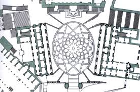
  Figure 2: Combining different symmetries

• QCD is the only local quantum field theory we have for “strong” forces. We must test our control over it quantitatively, by examining charm meson & baryon lifetimes, inclusive semi-leptonic branching ratios, etc.

• Measuring $D^{+}_{(s)}\to\mu^{+}\nu(+\gamma^{\prime}s)$, $\tau^{+}\nu(+\gamma^{\prime}s)$ provides us with superior tests of LQCD and also, perhaps, evidence for ND. For exclusive semi-leptonic decays, the scenarios are more complex, since long-distance dynamics are crucial. LQCD and other theoretical tools are furnished with very good test grounds.

• Very suppressed decays such as $D^{0}\to\gamma\gamma$, $D_{(s)}\to l^{+}l^{-}X$, etc., have not been found to date. This issue is dominated by long-distance dynamics over which we have little control. If sufficient large datasets were provided, we might learn from those rates. However, when we have to analyze refined asymmetries, we have an opportunity to determine the existence of ND [15].

• It is important to find CP asymmetries in two-body final states (FS) in mesons & baryons. However, it is crucial to probe regional CP asymmetries in three- & four-body FS. We have two examples with $B^{\pm}$ decays [16, 17]. The SM produces very small CP asymmetries in singly Cabibbo-suppressed (SCS) transitions and basically zero in doubly Cabibbo-suppressed (DCS) ones. In the latter we could find impact of ND with hardly one SM background.

The usual tools for strong-force investigations provide a good spectroscope for hadrons. However, when we include weak dynamics, more refined tools are required in order to probe CP asymmetries.

This article is organized as follows: in Section 2, I discuss local and global symmetries and the tools required for heavy hadron data analyses in general; I discuss (semi-)leptons and rare decays of charm hadrons in Section 3; then, in Section 4 I turn to the non-leptonic decays of charm hadrons. These provide a significantly more complex landscape, in particular regarding many-body FS. It is important to calibrate $\tau$ decays in $\Delta S=0,1$ for several reasons, as shown in Section 5. Comments about correlations with beauty transitions are given in Section 6. Finally, Section 7 summarizes the current status of the field and provides an outlook for the future.

2 Symmetries & tools

The flavor landscapes differ significantly for charm & beauty hadrons and $\tau$ leptons with different uncertainties. Obviously, beauty hadrons carry heavy flavor; however, charm hadrons and $\tau$ lepton mostly are on the right side of heavy flavor. In my view, there is a more general term: “symmetry” (= “$\sigma\upsilon\mu\mu\epsilon\tau\rho\alpha$”) goes beyond the meaning of “tools”.

2.1 Refined parametrization of CKM matrix

The dynamics of flavor violation in the SM world are described by the CKM matrix as the first step. The CKM matrix describes the quark couplings with left-handed charged bosons in terms of three angles and one weak phase with three families. The correlations between the matrix elements are described by three unity relations and six triangles, where the latter have the same area . We primarily focus on hadron decays, but the CKM matrix is also used for the productions of flavor hadrons with

$$\sum_{i=1}^{3}|V_{ij}|^{2}=1\;\; \;\;j=1,2,3,$$ ; (1)

$$\sum_{i=1}^{3}V_{ji}V^{*}_{ki}=0=\sum_{i=1}^{3}V_{ij}V^{*}_{ik}\; \;j,k=1,2,3,\;j\neq k,$$ ; (2)

$$|{\rm Im}V^{*}_{km}V_{lm}V_{kn}V^{*}_{ln}|=|{\rm Im}V^{*}_{mk}V_{ml}V_{nk}V^{*}_{nl}|=J {\rm area\,(every\,triangle)}=\frac{1}{2}J.$$ , (3)

In the SM with three quark families, these equalities are correct (excluding experimental uncertainties). The majority of researchers use the “smart” parametrization going back to Wolfenstein [18] with an obvious pattern although we did not understand its source. This approach involves three parameters: $A$, $\bar{\rho}$, and $\bar{\eta}$, which are assumed to be of order unity, and a known $\lambda={\rm sin}\theta_{C}\sim 0.22$, to be used for expansions in higher orders. This approach describes the flavor dynamics data quite well, including CP violation. This parametrization puts six triangles into three classes and is very successful:

$${\bf{\rm V}}_{\rm CKM}\simeq\left(\footnotesize\begin{array}[]{ccc}1-\frac{\lambda^{2}}{2}&\lambda,&A\lambda^{3}(\rho-i\eta+\frac{i}{2}\eta\lambda^{2})\\ -\lambda&1-\frac{\lambda^{2}}{2}-i\eta A^{2}\lambda^{4}&A\lambda^{2}(1+i\eta\lambda^{2})\\ A\lambda^{3}(1-\rho-i\eta)&-A\lambda^{2}&1\end{array}\right),$$ (7)

$${\rm`Old^{\prime}\,triangle\;I.1:} V_{ud}V^{*}_{us}\;\;\;[{\cal O}(\lambda)]+V_{cd}V^{*}_{cs}\;\;\;[{\cal O}(\lambda)]+V_{td}V^{*}_{ts}\;\;\;[{\cal O}(\lambda^{5})]=0,$$ (8)

$${\rm`Old^{\prime}\,triangle\;I.2:} V^{*}_{ud}V_{cd}\;\;\;[{\cal O}(\lambda)]+V^{*}_{us}V_{cs}\;\;\;[{\cal O}(\lambda)]+V^{*}_{ub}V^{*}_{cb}\;\;\;[{\cal O}(\lambda^{5})]=0,$$ (9)

$${\rm`Old^{\prime}\,triangle\;II.1:} V_{us}V^{*}_{ub}\;\;\;[{\cal O}(\lambda^{4})]+V_{cs}V^{*}_{cb}\;\;\;[{\cal O}(\lambda^{2})]+V_{ts}V^{*}_{tb}\;\;\;[{\cal O}(\lambda^{2})]=0,$$ (10)

$${\rm`Old^{\prime}\,triangle\;II.2:} V^{*}_{cd}V_{td}\;\;\;[{\cal O}(\lambda^{4})]+V^{*}_{cs}V_{ts}\;\;\;[{\cal O}(\lambda^{2})]+V^{*}_{cb}V^{*}_{tb}\;\;\;[{\cal O}(\lambda^{2})]=0,$$ (11)

$${\rm`Old^{\prime}\,triangle\;III.1:} V_{ud}V^{*}_{ub}\;\;\;[{\cal O}(\lambda^{3})]+V_{cd}V^{*}_{cb}\;\;\;[{\cal O}(\lambda^{3})]+V_{td}V^{*}_{tb}\;\;\;[{\cal O}(\lambda^{3})]=0,$$ (12)

$${\rm`Old^{\prime}\,triangle\;III.2:} V^{*}_{ud}V_{td}\;\;\;[{\cal O}(\lambda^{3})]+V^{*}_{us}V_{ts}\;\;\;[{\cal O}(\lambda^{3})]+V^{*}_{ub}V^{*}_{tb}\;\;\;[{\cal O}(\lambda^{3})]=0.$$ (13)

Fitting global 2014 data and using $\bar{\rho}=\rho(1-\lambda^{2}/2+...)$, etc., gives [19]

$$\lambda=0.22537\pm 0.00061\;\;\; \;\;\;A=0.814^{+0.023}_{-0.024},$$ , (14)

$$\bar{\rho}=0.117\pm 0.021\;\;\; \;\;\;\bar{\eta}=0.353\pm 0.013.$$ , (15)

However, one subtle problem occurs. The data suggests that $|\bar{\eta}|$ and $|\bar{\rho}|$ are not of order unity, with the latter being further removed. It is somewhat surprising how this obvious pattern is so successful, despite its disagreement with the expected values of $\bar{\eta}$ and $\bar{\rho}$. In the present era, accuracy and even precision are required. Other parametrizations have therefore been suggested and for good reasons. For example, the method proposed in Ref.[20] uses $\lambda$ with $f\sim 0.75$, $\bar{h}\sim 1.35$, and $\delta_{\rm QM}\sim 90^{o}$. This approach is close to reality as regards incorporating a non-leading source for $B$ decays and/or a very small source for $D$ decays in the SM, with

$$V_{\rm refined}=\left(\footnotesize\begin{array}[]{ccc}V_{ud}&V_{us}&V_{ub}\\ V_{cd}&V_{cs}&V_{cb}\\ V_{td}&V_{ts}&V_{tb}\end{array}\right)=\;\;\;\;\;\;\;\;\;\;\;\;\;\;\;\;\;\;\;\;\;\;\;\;\;\;\;\;\;\;\;\;\;\;\;\;$$ (19)

$$=\left(\footnotesize\begin{array}[]{ccc}1-\frac{\lambda^{2}}{2}-\frac{\lambda^{4}}{8}-\frac{\lambda^{6}}{16},&\lambda,&\bar{h}\lambda^{4}e^{-i\delta_{\rm QM}},\\ &&\\ -\lambda+\frac{\lambda^{5}}{2}f^{2},&1-\frac{\lambda^{2}}{2}-\frac{\lambda^{4}}{8}(1+4f^{2})-f\bar{h}\lambda^{5}e^{i\delta_{\rm QM}}&f\lambda^{2}+\bar{h}\lambda^{3}e^{-i\delta_{\rm QM}}\\ &+\frac{\lambda^{6}}{16}(4f^{2}-4\bar{h}^{2}-1),&-\frac{\lambda^{5}}{2}\bar{h}e^{-i\delta_{\rm QM}},\\ &&\\ f\lambda^{3},&-f\lambda^{2}-\bar{h}\lambda^{3}e^{i\delta_{\rm QM}}&1-\frac{\lambda^{4}}{2}f^{2}-f\bar{h}\lambda^{5}e^{-i\delta_{\rm QM}}\\ &+\frac{\lambda^{4}}{2}f+\frac{\lambda^{6}}{8}f,&-\frac{\lambda^{6}}{2}\bar{h}^{2}\\ \end{array}\right)+{\cal O}(\lambda^{7}).$$ (27)

Thus, the landscape of the CKM matrix is more subtle than usually stated; it is described by six triangles that differ subtly in ways, but retain the same area. Therefore,

$${\rm Triangle\;I.1:} V_{ud}V^{*}_{us}\;\;\;[{\cal O}(\lambda)]+V_{cd}V^{*}_{cs}\;\;\;[{\cal O}(\lambda)]+V_{td}V^{*}_{ts}\;\;\;[{\cal O}(\lambda^{5\&6})]=0,$$ (28)

$${\rm Triangle\;I.2:} V^{*}_{ud}V_{cd}\;\;\;[{\cal O}(\lambda)]+V^{*}_{us}V_{cs}\;\;\;[{\cal O}(\lambda)]+V^{*}_{ub}V^{*}_{cb}\;\;\;[{\cal O}(\lambda^{6\&7})]=0,$$ (29)

$${\rm Triangle\;II.1:} V_{us}V^{*}_{ub}\;\;\;[{\cal O}(\lambda^{5})]+V_{cs}V^{*}_{cb}\;\;\;[{\cal O}(\lambda^{2\&3})]+V_{ts}V^{*}_{tb}\;\;\;[{\cal O}(\lambda^{2})]=0,$$ (30)

$${\rm Triangle\;II.2:} V^{*}_{cd}V_{td}\;\;\;[{\cal O}(\lambda^{4})]+V^{*}_{cs}V_{ts}\;\;\;[{\cal O}(\lambda^{2\&3})]+V^{*}_{cb}V^{*}_{tb}\;\;\;[{\cal O}(\lambda^{2\&3})]=0,$$ (31)

$${\rm Triangle\;III.1:} V_{ud}V^{*}_{ub}\;\;\;[{\cal O}(\lambda^{4})]+V_{cd}V^{*}_{cb}\;\;\;[{\cal O}(\lambda^{3\&4})]+V_{td}V^{*}_{tb}\;\;\;[{\cal O}(\lambda^{3})]=0,$$ (32)

$${\rm Triangle\;III.2:} V^{*}_{ud}V_{td}\;\;\;[{\cal O}(\lambda^{3})]+V^{*}_{us}V_{ts}\;\;\;[{\cal O}(\lambda^{3\&4})]+V^{*}_{ub}V^{*}_{tb}\;\;\;[{\cal O}(\lambda^{4})]=0.$$ (33)

The pattern in flavor dynamics is less obvious for CP violation in hadron decays, as stated previously [21]. Triangles III.1, II.1, and I.1 describe $B^{0}$, $B^{0}_{s}$, and $K^{0}$, respectively, including oscillations. Super-heavy top quarks decay before they can produce hadrons [9], and Triangle I.2 affects charm transitions. SCS transitions provide a more complex scenario, as can be seen in $c\to du\bar{d}$, $c\to su\bar{s}$ diagrams and $c\Rightarrow u$ transitions. The latter poses a veritable challenge as regards connecting quark diagrams with hadronic amplitudes; for example, the difference between penguin diagrams and final state interactions (FSI)/re-scattering is “fuzzy”. Furthermore, we must consider interference between Cabibbo-favored & DCS amplitudes.

The correlations between triangles are very important; for example, $c\to du\bar{s}$ describes DCS amplitudes in mesons & baryons and gives zero weak phases up to ${\cal O}(\lambda^{7})$. I will discuss this and connections with beauty hadron transitions below. This is only the first step in discussing the information that the data give us. A second step is also required, which involves both work and judgment. A third step is necessary, in which additional data, tools, time, and thinking are required.

2.2 Adler-Bell-Jackiw (ABJ) (or triangle) anomaly

In the world of three quark and two lepton families, another subtle challenge had to be overcome. A classical symmetry is expressed because of the existence of a conserved current; we obtain $\partial^{\mu}J^{5}_{\mu}=0$ for massless fermions. However, the triangle diagram with an internal loop of only fermions coupled to three external axial vectors or one axial & two vectors generates a “quantum anomaly”; i.e., it removes a classical symmetry [22]:

$$\partial^{\mu}J^{5}_{\mu}=\frac{g_{S}^{2}}{16\pi^{2}}G\cdot\tilde{G}\neq 0,$$ (34)

even for massless fermions. $G$ and $\tilde{G}$ denote the gluonic field strength tensor & its dual, where $\tilde{G}_{\mu\nu}=\frac{i}{2}\epsilon_{\mu\nu\rho\sigma}G^{\rho\sigma}$. $G\cdot\tilde{G}\neq 0$ by itself yields a finite result, yet it destroys the renormalizability of the theory. That is, it cannot be “renormalized away” in a gauge-invariant manner with a dimensional four operator. Instead, it must be neutralized by adding a contribution from all fermion classes in the theory to obtain a zero result. For the SM, the sum of all electric charges of fermions of a given family must be zero. This imposes a connection between the quark & lepton charges, i.e., $e$ & $\mu$ have charge number “-2”, and the $u,d,s$ quarks with three colors “0”; however, with colored charm quarks we obtain “+2”. This result is excellent, yet the connection is unexplained. Another challenge exists, as we have found that the $\tau$ lepton adds another charge number “-1” with a mass similar to those of charm mesons. Therefore, some researchers expected to find the third family of quarks, namely, $[t,b]$, with significantly heavier masses. This indicates that Nature has a sense of humor to deal with our understanding or lack of it.

There are three points to note here: (a) The impact of the “ABJ anomaly” has an unusually long history in modern physics: these important papers were published over 45 years ago [22]. (b) This anomaly did not only have theoretical implications. It also had an impact in the real world, in relation to the $\pi^{0}\to 2\gamma$ decay in particular. In fact, an even older paper by Nobel Prize Winner J. Steinberger [23] discusses this point. (c) The “ABJ anomaly” is not primarily relevant in terms of history; one learns from the theoretical techniques used previously and applied in other landscapes.

2.3 Theoretical tools for decays

I assume CPT invariance, analyticity, & unitarity in quantum field theory (& also in effective theories). These connections are subtle in many ways. There are three classes of FS for hadrons: leptonic, semi-leptonic, and non-leptonic . Furthermore, there are both inclusive and exclusive subclasses, where different tools (with different uncertainties) can be used. I will return to this topic below and discuss it in some detail. The same classifications apply to the decays of both charm & beauty hadrons, although the details differ; for example, Dalitz plots for three-body FS are primarily populated with charm decays, while the center is basically empty of beauty hadrons. Finally, one can and should use semi-hadronic $\tau$ decays to calibrate predictions with real data.

Quark diagrams are described with two-dimensional plots; however, in general, the FS are described by three-dimensional plots (and beyond, when one includes spin observables). To be realistic, it is sufficient to discuss nonleptonic decays with four-body FS at most. Furthermore, the connections between quark diagrams and operators are subtle, particularly as regards local and non-local operators. Note that the latter depend crucially on long-distance FSI. I will discuss these classes in more detail below.

• First, one focuses on two-body non-leptonic FS. These states give one-dimensional observables from the rates and numbers of CP asymmetries.

• Probing Dalitz plots for CP asymmetries gives two-dimensional observables, as we have previously seen regarding $B$ decays. I will comment on this below. If the plot is not flat, it indicates that the FSI are not trivial, and are similar to resonances in different ways. One applies amplitudes for FS with hadrons and resonances, with $P\to h_{1}[h_{2}h_{3}]+h_{2}[h_{1}h_{3}]+h_{3}[h_{1}h_{2}]\Rightarrow h_{1}h_{2}h_{3}$ . I am not claiming that three-body amplitudes are perfectly described by a sum of two-body FS. However, this approach is sufficient to a large extent, realistically speaking.

  As a second step that the analyses are model-insensitive . However, we must remember that the real theory does not always yield the best fitting of the data. Furthermore, we must measure correlations with other data. We have the tools to measure regional asymmetries in Dalitz plots. First, one uses model-insensitive tools, and then real theoretical tools that are validated based on correlations with other transitions are applied. Thus, these theoretical tools must be “acceptable”. Note that the criteria determining acceptability vary.

• One must be realistic with finite data when probing four-body FS and identify tools to analyze one-dimensional asymmetries. We are at the beginning of the road towards understanding the underlying forces.

The real impact of ND will become apparent in detailed discussion.

Connections between effective quark operators and hadronic transitions due to “duality” exist [24] – however, they are subtle. One cannot compare the FS using measured hadron masses and suggested mass values for quarks only; this neglects the crucial point of duality, i.e., the impact of non-perturbative forces.

The landscapes of CP asymmetries in charm (& beauty) hadrons provide a “wonderful challenge” for probing ND (including baryon decays [25]). At minimum, we learn about the impact of FSI in the world of hadrons.

For several reasons, the number of colors must be three (specifically, neither two nor four). Yet, in the limit of $N_{C}\to\infty$, QCD’s non-perturbative dynamics becomes tractable [26]. Thus, only planar diagrams contribute to hadronic scattering, and the asymptotic states are $\bar{q}q=$ mesons & $qqq=$ baryons. “Confinement” is then proven (also $\bar{q}q\bar{q}q$, etc.). Further, the Zweig or OZI rule holds. One treats short-distance dynamics with $N_{C}=3$ fixed, so as to derive an effective Lagrangian at lower scales. Once the Lagrangian has been devolved to the scale at which one wishes to evaluate the hadronic matrix elements, which are shaped by long-distance dynamics, one expands the matrix elements in powers of $1/N_{C}$ for $H_{Q}\to f$, such that

$$\langle f|{\cal L}_{\rm eff}|H_{Q}\rangle\propto b_{0}+\frac{b_{1}}{N_{C}}+{\cal O}(1/N_{C}^{2}).$$ (35)

This expansion of $N_{C}\to\infty$ has often indicated the aforementioned directions for future research. For example, it has aided researchers in treating two-body non-leptonic decays of charm mesons [13, 27]. This technology lies between models where one can discuss uncertainties inside the model and real theories, where the uncertainties can be decreased systematically. It is not truly an expansion, since it cannot go beyond $b_{1}$.

2.3.1 Effective transition amplitudes including re-scattering

One can describe the amplitudes of hadrons with CPT invariance following the history outlined above; it is given in detail in Refs.[28, 29] and in Sect. 4.10 of Ref.[30].

$$T(P\to f) = e^{i\delta_{f}}\left[T_{f}+\sum_{f\neq a_{j}}T_{a_{j}}iT^{\rm resc}_{a_{j}f}\right],$$ (36)

$$T(\bar{P}\to\bar{f}) = e^{i\delta_{f}}\left[T^{*}_{f}+\sum_{f\neq a_{j}}T^{*}_{a_{j}}iT^{\rm resc}_{a_{j}f}\right]\;,$$ (37)

where $T^{\rm resc}_{a_{j}f}$ describe the FSI between $f$ and intermediate on-shell states $a_{j}$ that connect with this FS. It is generally sufficient to focus on strong re-scattering; one can label it simply FSI. One obtains “regional” CP asymmetries and not only “averaged” results, with

$$\Delta\gamma(f)=|T(\bar{P}\to\bar{f})|^{2}-|T(P\to f)|^{2}=4\sum_{f\neq a_{j}}T^{\rm resc}_{a_{j}f}\,{\rm Im}T^{*}_{f}T_{a_{j}}\;.$$ (38)

CP asymmetries must vanish upon summing over all such $f$ states using CPT invariance between subclasses of partial widths, where

$$\sum_{f}\Delta\gamma(f)=4\sum_{f}\sum_{f\neq a_{j}}T^{\rm resc}_{a_{j}f}\,{\rm Im}T_{f}^{*}T_{a_{j}}=0\;,$$ (39)

since $T^{\rm resc}_{a_{j}f}$ & Im$T_{f}^{*}T_{a_{j}}$ are symmetric & antisymmetric, respectively, in the indices $f$ & $a_{j}$.

These FS $f$ consist of two-, three-, four-body states, etc., such as pions and kaons. One describes three-body FS using Dalitz plots, whereas the landscapes of four-body states, etc., are even more “complex”, being essentially a “drama with more actors”. In principle, one can probe local asymmetries, however, one must be realistic regarding finite data and a lack of “perfect” quantitative control of non-perturbative QCD. The first step is to use models for looking at the data; the second step is to analyze model-insensitive ways. Finally we should not be “slaves” of the best fits of the data. Instead, we require real theories providing understanding of the underlying dynamics. We must also consider the correlations between our obtained data and interpret them in an acceptable manner. This statement is subtle (and also concerns the definition of “regional” asymmetries), but crucial. I will discuss these points in some detail below.

We can describe transitions of boundstates of $\bar{q}q$ (or $qqq$); the simplest case is for mesons, but it is not simple. We must include re-scattering due to strong forces and its large impact. Penguin diagrams can account for absorption due to internal $c$ quarks in principle by adding pairs of $\bar{q}q$ for beauty hadrons. However the cases involving charm hadrons are unclear, even in principle. The connections of penguin and tree diagrams with reality are often fuzzy, as pointed out in Refs. [28, 29, 30].

Can we quantitatively connect quark diagrams with hadronic amplitudes? It is one thing to draw quark diagrams by adding pairs of $\bar{q}q$, but trusting them is a completely separate issue. How can one connect data concerning decays for two-, three-, four-body FS with information about the underlying dynamics? We must apply several theoretical tools in this case, which must be connected with other transitions, and we must also consider their limits. Here, I will discuss U-spin symmetry, focusing on its uncertainties and its connections with the V-spin case. I will also comment briefly on dispersion relations.

Penguin diagrams show amplitudes for $Q\to q+$ gluons, where $Q$ and $q$ quarks carry the same charge; consider the artistic version shown in Fig.3 with large solid quark lines and wavy lines for $W^{\pm}$ plus one gluon.

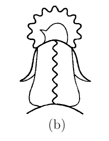
Figure 3: Artistic diagrams of penguin amplitudes; the picture of the (b) diagram was reproduced from Parity by permission of T. Muta & T. Morozumi

Ignoring artistic ambition, penguin diagrams are satisfactory as regards $b$ (& $s$) quarks. However, one should not hide theoretical uncertainties; furthermore, different scenarios exist: $b\Rightarrow s,\,d$ amplitudes are given by local or short-distance operators and have a sizable impact on inclusive rates. For exclusive rates, however, we have less control. On the other hand, we have $c\Longrightarrow u$ amplitudes, which are mostly dominated by long-distance dynamics, where we have less control over inclusive rates and significantly less control over exclusive rates. Based on chiral symmetries, one expects them to primarily affect two-body FS and to have some influence on three-body FS, but hardly beyond. Re-scattering amplitudes include the impact of penguin diagrams, but their landscapes are significantly broader:

• Eqs. (36,37) apply to amplitudes in general, including many-body FS, whether for hadron or quark boundstates (with constitute quarks) in initial states (& between). This is regardless of whether or not we can perform this calculation.

• The manner in which one can connect the hadronic and quark amplitude landscapes depends on various factors. One hopes to be sufficiently removed from the $\bar{c}c$ threshold to produce $\Delta\Gamma(B_{s,d})$ for $B_{s,d}$ primarily through short-distance dynamics; this has also been somewhat suggested for $\Delta\Gamma(D^{0})$, perhaps. When one discusses direct CP asymmetries, one requires both weak & strong phases. Quark amplitudes give weak phases, while penguin diagrams from non-local operators provide the imaginary component that one requires for (strong) re-scattering. However, SCS transitions of charm hadrons are very complex. There is a difference between diagrams one can compute and amplitudes that are measurable because of interference including re-scattering.

• A general statement can be made. Since our control of strong dynamics is quite limited quantitatively (at present), “global” strong phases are very often used to discuss data concerning three- & four-body FS. It is claimed that accurate information can be obtained in this manner. However, this is only the first step.

• Penguin diagrams do not affect DCS decays of $D_{(s)}$ & $\Lambda_{c}^{+}$, while re-scattering does.

• We require the aid of refined tools like dispersion relations to understand the information provided by the data. I will discuss these items below.

We must consider which theoretical tools we can apply and their limits. Obviously, chiral symmetry is an excellent candidate, although some subtle points must be considered. U-spin symmetry is a “popular” candidate. However, I have grave concerns regarding the control of theoretical uncertainties, in particular by ignoring the connections between U- & V-spin symmetries and, even worse, FS with only charged hadrons. I will discuss this problem below.

2.3.2 Connections of U- & V-spin symmetries: spectroscopy vs. weak decays

The global (& broken) $SU(3)_{fl}$ with its three subsymmetries $SU(2)_{I}$, $SU(2)_{U}$, & $SU(2)_{V}$ was introduced first, when “constituent” quarks were primarily seen as mathematical tools to describe the hadron spectroscopies rather than real physical states. They are applicable to spectroscopy and can be used to discuss baryon and meson masses, although the latter are significantly affected by chiral symmetry. When one compares the masses of nucleons, $\Lambda$ and $\Xi$, one can suggest the values of the constituent quark masses, where $m_{u}^{\rm const}\simeq m_{d}^{\rm const}\sim 0.3$ GeV & $m_{s}^{\rm const}\sim 0.5$ GeV [31]. Now, we can compare the masses of charm baryons; i.e., $M(\Lambda_{c}^{+})\simeq 2.29$ GeV vs. $M(\Xi_{c}^{+})\simeq 2.46$ GeV and $M(\Xi_{c}^{0})\simeq 2.47$ GeV vs. $M(\Omega_{c}^{0})\simeq 2.7$ GeV. One obtains differences of $\sim 0.2$ GeV in both cases; therefore, this approach is satisfactory, but this is not an accurate tool. We have a better understanding of this: the mixing of $\langle 0|\bar{u}u|0\rangle$, $\langle 0|\bar{d}d|0\rangle$ between $\langle 0|\bar{s}s|0\rangle$ with scalar resonances are not OZI suppressed [32]. It makes sense to use U-spin symmetry when considering the spectroscopy of charm & beauty hadrons. However, these situations are more complex when one combines strong & weak dynamics.

Re-scattering has an important impact on weak amplitudes in general and on CP asymmetries in particular (see Eqs. (36 - 38)) [28, 29, 30]. We cannot ignore the correlations of U-spin with V-spin symmetries. In other words, one cannot focus on two-body FS or even more with only charged particles in weak transitions. Simple situations appear in very low-energy collisions of $K^{-}\pi^{+}\Leftrightarrow\bar{K}^{0}\pi^{0}$ using $SU(2)_{I}$ symmetry and even $K^{-}\pi^{+}\Leftrightarrow\bar{K}^{0}\eta$. However, at somewhat higher energies one must discuss re-scattering, primarily regarding $K\pi\to K2\pi,\,K3\pi$, and even $\pi K\to 3K,\,3K\pi$, etc., where obvious differences between the initial and final states exist. This also changes $\pi^{+}\pi^{-}\Leftrightarrow\pi^{0}\pi^{0}$ at very low energies. However, the situation changes significantly at slightly higher energies, with $\pi^{+}\pi^{-}/\pi^{0}\pi^{0}/\pi^{+}\pi^{0}\to 4\pi...$ because of G-parity. Furthermore, this affects $\pi\pi\Leftrightarrow\bar{K}K$ at very low energies, but the landscape is also $\pi\pi\to K\bar{K}\pi,K\bar{K}2\pi,K\bar{K}K\bar{K}$ at somewhat higher energies.

There are very different time scales for weak vs. strong forces. Therefore strong re-scattering has a large impact; it makes the differences between U- & V-spin symmetries very fuzzy. Obviously, U-spin symmetry is broken significantly. The first guess is $(M_{K}^{2}-M^{2}_{\pi})<(M_{K}^{2}+M^{2}_{\pi})$, and more refined solutions are based on the constituent quarks. One can use this approach for models to predict exclusive decays, but with large theoretical uncertainties; the problem lies in treating the FSI quantitatively. In particular, we have the tools to probe Dalitz plots with like dispersion relations. The only problems we must face are the requirements for more data and more time to analyze these findings and to check them against correlations with other transitions. I will return to this topic and discuss it in some detail below.

In the world of quarks, one describes primarily inclusive transitions. “Current” quarks with $m_{u}<m_{d}<<m_{s}$ are based on theory. I-, U- , & V-spin symmetries consider $u\leftrightarrow d$, $d\leftrightarrow s$, & $u\leftrightarrow s$, respectively. These three symmetries are obviously broken on different levels, and these violations are connected in the SM. The operators producing inclusive FS depend on their CKM parameters and the current quark masses involved there. However, the real scale for inclusive decays is given by the impact of QCD, i.e., $\bar{\Lambda}\sim 1$ GeV . Thus, the violations of U- & V-spin symmetries are small, and tiny for the I-spin case. We can deal with inclusive rates of beauty and, perhaps, charm hadrons using effective operators in the world of quarks.

The connections between inclusive and exclusive hadronic rates are not obvious, particularly as regards quantitative techniques. The violations of I-, U-, & V-spin symmetries in the measurable world of hadrons are expected to be scaled by the differences in pion and kaon masses, which are not small compared to $\bar{\Lambda}$ (or $[m^{2}_{K}-m^{2}_{\pi}]/[m^{2}_{K}+m^{2}_{\pi}]$). This is even more crucial in terms of direct CP violation and the impact of strong re-scattering on amplitudes.

Returning to the history of this field, Lipkin suggested that U-spin violations in $B$ decays are of the order of 10–20 % [33] in CKM-favored cases, and may be larger in suppressed cases. One reason for this is that suppressed decays in the world of hadrons consist of larger numbers of states in the FS, where strong FSI with opposite signs have significant impact. Furthermore, the worlds of hadrons (or constitute quarks) are controlled by FSI because of non-perturbative QCD; they have the strongest impact on exclusive cases. For good reasons, it has been stated that violation of U-spin symmetry is approximately ${\cal O}(10\%)$ in inclusive decays. In the sum of exclusive decays, large ratios that fluctuate more significantly can be seen, and I will discuss well-known examples of this below. My central point is that we cannot discuss U-spin symmetry (& its violations) singly; instead, we must discuss connections with V-spin symmetry.

2.4 Expansions

Usually, we cannot truly solve the challenges we face in the QFT landscapes. Many of the best theoretical tools we have are based on certain expansions, where some systematic uncertainties exist . I am not saying that we cannot use models; however, this is the first step being taken in the 21st century and the research direction should be changed, based on improved data and more careful thinking. Models have no systematic limits.

I will mention a special case, namely, QCD. First, there is no competition from any other local gauge theory. It is not trivial at all to combine truly strong forces in long distances with asymptotic freedom at short distances using this approach. Further, QCD is crucial to combine self-interactions of three and four gluons with their color quarks, and it is much easier to draw diagrams with gluon-quark couplings. However, one then overlooks the crucial point of non-abelian gauge theories.

2.4.1 Heavy quark theory

The lack of full calculational control of strong forces limits our understanding of the information given by the data. We require other tools, such as chiral theory, to consider non-perturbative dynamics in special settings. We have heavy-quark symmetry (HQS). The non-relativistic dynamics of a spin-$\frac{1}{2}$ particle with charge $g$ is described by the Pauli Hamiltonian

$${\cal H}_{\rm Pauli}=-gA_{0}+\frac{(i\vec{\partial}-g\vec{A})^{2}}{2m}+\frac{g\vec{\sigma}\cdot\vec{B}}{2m},$$ (40)

where $A_{0}$ & $\vec{A}$ denote the scalar & vector potentials and the magnetic field is $\vec{B}$. In the heavy mass limit, only the first term survives, such that

$${\cal H}_{\rm Pauli}\to-gA_{0}\;\;{\rm as}\;\;m\to\infty\;,$$ (41)

i.e., an infinite heavy “electron” is static. It does not propagate, instead it interacts only via the “Coulomb” potential and its spin dynamics become decoupled.

This is also the case for an infinite heavy quark. Its mass is separate from its dynamics (although not its kinematics), and it is the source of a static color Coulomb field that is independent of the heavy-quark spin. That is the statement made by the HQS. There are several direct consequences of the heavy-light system spectrum, i.e., mesons = $[Q\bar{q}]$ and baryons = $[Qq_{1}q_{2}]$. First, in the limit of $m_{Q}\to\infty$, the spin of the heavy quark $Q$ decouples, and the spectra of the heavy-flavor hadrons are described in terms of the spin and orbital degrees of freedom of the light quarks alone. Therefore, to leading order accuracy, one obtains no hyperfine splitting and

$$M_{D}\simeq M_{D^{*}}\;,\;M_{B}\simeq M_{B^{*}}.$$ (42)

Simple scaling laws concerning the approach to the asymptote apply, where

$$M_{B^{*}}-M_{B} \sim \frac{m_{c}}{m_{b}}(M_{D^{*}}-M_{D}),$$ (43)

$$M_{B}-M_{D} \sim m_{b}-m_{c}.$$ (44)

It is obvious already from the spectroscopy results that beauty hadrons are heavy flavor; however, charm hadrons also primarily act as heavy-flavor particles.

For the heavy quark expansion (HQE), one requires dimensionless parameters to define the landscape, i.e., of the order of the ratio $\bar{\Lambda}/m_{Q}$, where $\bar{\Lambda}$ defines the short- vs. long-distance dynamics in heavy-flavor decays in QCD. $\bar{\Lambda}$ is usually also applied in LQCD analyses with ${\cal O}(1)$ GeV (or more). This depends on the case to which it is applied. Furthermore, subtle points should be made regarding the definition of quark masses: one uses the “running” mass $m_{Q}(\mu)$, defined at a scale of $\mu$ to shield it against strong infrared dynamics. One must use “well-defined” masses for decays, and not pole masses. However, we require additional tools.

2.4.2 Operator product expansion

Operator product expansion (OPE) (à la Wilson [34] ) provides a powerful theoretical tool of wide applicability.

• One defines a field theory ${\cal L}(\Lambda_{\rm UV})$ at a high ultraviolet scale $\Lambda_{\rm UV}$, which is significantly higher than $M_{W}$, $m_{Q}$, etc.

• One renormalizes the ${\cal L}$ from the cutoff $\Lambda_{\rm UV}$ down to the physical scale $\Lambda_{\rm phys}$ for application. In doing so, one integrates out the heavy degrees of freedom. That is, with like $M_{W}$ one arrives at an effective low-energy field theory using OPE, where

  $${\cal L}(\Lambda_{\rm UV})\to{\cal L}(\Lambda_{\rm phys})=\sum_{i}c_{i}(\Lambda_{\rm phys},\Lambda_{\rm UV},M_{W},...){\cal O}_{i}(\Lambda_{\rm phys}).$$ (45)

  The local operators ${\cal O}_{i}(\Lambda_{\rm phys})$ contain the active dynamical fields; i.e., those with frequencies below ${\cal O}_{i}(\Lambda_{\rm phys})$.

• Their coefficients $c_{i}(\Lambda_{\rm phys},\Lambda_{\rm UV},M_{W},...)$ provide the gateway for heavy degrees of freedom with frequencies above ${\cal O}_{i}(\Lambda_{\rm phys})$ to enter. They are shaped by short-distance dynamics and are usually computed perturbatively.

• Lowering the value of ${\cal O}_{i}(\Lambda_{\rm phys})$ changes the “shape” of the Lagrangian, such that ${\cal O}_{i}(\Lambda^{(1)}_{\rm phys})\neq{\cal O}_{i}(\Lambda^{(2)}_{\rm phys})$ for $\Lambda^{(1)}_{\rm phys}\neq\Lambda^{(2)}_{\rm phys}$. Integrating out heavier fields will induce higher-dimensional operators to emerge in the Lagrangian.

• As a matter of principle, observables cannot depend on the choice of $\Lambda_{\rm phys}$. They provide a demarcation line only, with

  $${\rm short\;distance}\;\;<\;\;1/\Lambda_{\rm phys}\;\;<\;\;{\rm long\;distance}.$$ (46)

  In practice, the value of $\Lambda_{\rm phys}$ must be chosen judiciously, because of the present limitations of our computational powers. It is reasonable to pick $\Lambda_{\rm phys}=\bar{\Lambda}\sim 1$ GeV, for application to charm transitions in particular.

We require additional & subtle steps for inclusive weak decays. One describes the decays into sufficiently inclusive final states in the weak interactions, using the imaginary part of the forward scattering operator up to second order accuracy and invoking the optical theorem. Thus,

$$T(Q\to Q)={\rm Im}\int d^{4}x\;i\{{\cal L}(x){\cal L}(0)\}_{t}\;,$$ (47)

with the subscript $t$ denoting the time-ordered product and ${\cal L}_{W}$ the relevant weak Lagrangian. $T(Q\to Q)$ represent, in general, a non-local operator. The space-time separation $x$ is given by the inverse of the energy release. If the latter is large compared to typical hadronic scales, the product is dominated by short-distance dynamics and one can apply an OPE. This yields an infinite series of local operators of increasing dimensions.

We take the $H_{Q}$ expectation values of the operator $T$ normalized by $2M_{H_{Q}}$, such that

$$\frac{\langle H_{Q}|{\rm Im}\,T(Q\to Q)|H_{Q}\rangle}{2M_{H_{Q}}} \propto$$ (48)

$$\propto\Gamma(H_{Q}\to f) = \frac{G_{F}^{2}m_{Q}^{5}(\omega)}{192\pi^{3}}|V_{\rm CKM}|^{2}\cdot$$ (49)

$$\cdot[c_{3}^{(f)}(\omega)\frac{\langle H_{Q}|\bar{Q}Q|H_{Q}\rangle_{(\omega)}}{2M_{H_{Q}}} + \frac{c_{5}^{(f)}(\omega)}{m_{Q}^{2}}\frac{\langle H_{Q}|\bar{Q}\frac{i}{2}\sigma\cdot GQ|H_{Q}\rangle_{(\omega)}}{2M_{H_{Q}}}+$$ (50)

$$+ \sum_{i}\frac{c_{6,i}^{(f)}(\omega)}{m_{Q}^{3}}\frac{\langle H_{Q}|(\bar{Q}\Gamma_{i}q)(\bar{q}\Gamma_{i}Q|H_{Q}\rangle_{(\omega)}}{2M_{H_{Q}}}+{\cal O}(1/m_{Q}^{4})].$$ (51)

One uses $\Lambda_{\rm phys}\ll\omega\ll m_{Q}$ for expansion to deal with the impact of perturbative & non-perturbative QCD. Short-distance dynamics shape the number of coefficients $c_{i}^{(f)}$. In practice, they are evaluated in perturbative QCD; they also provide the portals for ND entering naturally. Non-perturbative contributions enter through the expectation values of operators with dimensions of five & higher, i.e., $\bar{Q}\frac{i}{2}\sigma\cdot GQ$, $(\bar{Q}\Gamma_{i}q)(\bar{q}\Gamma_{i}Q)$, etc. Expanding the expectation value of the leading operator $\bar{Q}Q$ of dimension three, we obtain

$$\frac{1}{2M_{H_{Q}}}\langle H_{Q}|\bar{Q}Q|H_{Q}\rangle_{(\omega)} = 1-\frac{\mu^{2}_{\pi}(\omega)}{2m_{Q}^{2}}+\frac{\mu_{G}(\omega)}{2m_{Q}^{2}}+{\cal O}(1/m_{Q}^{3}),$$ (52)

$$\mu^{2}_{\pi}(\omega) = \frac{1}{2M_{H_{Q}}}\langle H_{Q}|\bar{Q}\vec{\pi}^{2}Q|H_{Q}\rangle_{(\omega)},$$ (53)

$$\mu^{2}_{G}(\omega) = \frac{1}{2M_{H_{Q}}}\langle H_{Q}|\bar{Q}\frac{i}{2}\sigma\cdot GQ|H_{Q}\rangle_{(\omega)}.$$ (54)

Observables cannot depend on the value of $\omega$. A crucial difference exists between amplitudes as, in real quantum field theories (QFT), it is not trivial to connect short- & long-distance dynamics. However, we do have the tools to accomplish this, as it is possible to discuss uncertainties only inside models of strong forces.

Inclusive transitions can be described in the $\bar{\Lambda}/m_{Q}$ expansion. We have learned that inclusive transitions begin only at the second order in general, for subtle reasons [35], which are related to lifetimes and semi-leptonic decays in particular. There are five points to note:

• For heavy flavor hadrons, the leading source of inclusive transitions is parton models in smart ways.

• Non-perturbative dynamics enter to the second order of $\bar{\Lambda}/m_{Q}$ only (also in smart ways).

• For the landscape of $H_{Q}$ transitions, we have the same list of operators: $\bar{Q}Q$, $\bar{Q}\frac{i}{2}\sigma\cdot GQ$, $(\bar{Q}\Gamma_{i}q)(\bar{q}\Gamma_{i}Q)$, etc., for the widths and distributions. However, their impact is very different due to subtle effects [36]. This is effective for the widths of beauty and charm hadrons, but not for charm hadron distributions.

• HQE functions significantly better than previously expected (again in smart ways).

• There is a large difference between inclusive and exclusive transitions. We expect this difference, but it is barely within our control.

The above makes sense for beauty decays, but what of $\bar{\Lambda}/m_{c}$? Obviously, it depends on the heavy quark mass. Note that one cannot use “pole mass” because of “old renormalon” uncertainties [37]. One must use a very effective definition, called “kinetic” mass [38, 37], where

$$\frac{dm_{Q}^{\rm kin}(\omega)}{d\omega}=-\frac{16\alpha_{S}(\omega)}{3\pi}-\frac{4\alpha_{S}}{3\pi}\frac{\omega}{m_{Q}}+...,$$ (55)

with a scale of $\sim 1$ GeV; this functions very well, including at least third & fourth order results. We require a little luck for application to charm hadrons; in poetic terms, we can accomplish it with “undue incantation”. Actually, the connection with lattice QCD studies gives us novel information concerning underlying fundamental dynamics, which is being tested now and will continue to be examined in the future.

The leading non-perturbative corrections arise at ${\cal O}(1/m_{Q}^{2})$ and differentiate between baryons on one side and mesons on the other; the latter have practically the same values. In ${\cal O}(1/m_{Q}^{3})$, the landscapes also differentiate between mesons with dimension six operators. One describes Pauli interferences (PI) that are negative for mesons, but not for baryons in general. Weak annihilation/exchanges (WA) have a sizable impact on baryon amplitudes. We have acquired information even from the ${\cal O}(1/m_{Q}^{4})$ contribution and have made some estimates concerning the ${\cal O}(1/m_{Q}^{5})$ case. One must have realistic expectations regarding charm decays.

2.5 Sum rules and dispersion relations

Other less “famous” theoretical tools exist. They are also important and will be even more so in the future, when we will be forced to focus on accuracy.

2.5.1 Sum rules

“Sum rules” are ubiquitous tools in many branches of physics, involving sums or integrals over observables such as rates & their moments, etc. A celebrated case is the SVZ QCD sum rules named after Shifman, Vainshtein, & Zakharov [39], which allow low-energy hadronic quantities to be expressed through basic QCD parameters. An OPE is obtained, and non-perturbative dynamics are then parametrized through condensates $\langle 0|\bar{q}q|)\rangle$, $\langle 0|GG|0\rangle$, etc. They are zero in perturbative QCD; however, they are treated as free parameters, the values of which are fitted from certain observables. This approach also indicates that the duality between the worlds of the hadrons & quarks (& gluons) is not always local, i.e., we must treat “smeared” hadronic observables. The first real example is the description of $e^{+}e^{-}\to\gamma^{*}\to$ hadrons in the energy range $E_{c.m.}\sim 3.6-5$ GeV, including narrow resonances.

One can also apply “light-cone sum rules” [40], “small velocity (SV)” [41], and “spin sum rules” [42]. Certain examples exist to which the OPE is applicable:

$$\mu^{2}_{G}(\omega) \leq \mu_{\pi}^{2}(\omega),$$ (56)

$$\mu^{2}_{G}(1\,{\rm GeV}) \simeq \frac{3}{2}[M^{2}_{B^{*}}-M^{2}_{B}]\simeq 0.35\pm 0.03\;({\rm GeV})^{2},$$ (57)

$$\mu_{\pi}^{2}(1\;{\rm GeV}) \simeq 0.45\pm 0.1\;{\rm(GeV)^{2}}.$$ (58)

The OPE is applicable through ${\cal O}(1/m_{Q}^{3},1/m_{Q}^{4})$ (and more [43]) for beauty decays. This approach is also surprisingly applicable to charm transitions, through ${\cal O}(1/m_{c}^{3})$.

2.5.2 Dispersion relations

Dispersion relations [44, 32] are encountered in many branches of physics and in quite different contexts; they are based on the general validity of central statements in QFT. We can relate the values of a two-point function $\Pi(q^{2})$ in a QFT at different complex values of $q^{2}$ to each other through an integral representation. In particular, one can evaluate $\Pi(q^{2})$ for large Euclidean values with the help of an OPE, and then relate the coefficients $I_{n}^{\rm OPE}$ of local operators $O_{n}$ to observables such as $\sigma(e^{+}e^{-}\to{\rm hadrons})$ & their moments in the physical, i.e., Minkowskian domain. This is achieved by taking an integral over the discontinuity around the real axis, such that

$$I_{n}^{\rm OPE}\simeq\frac{1}{\pi}\int_{0}^{\infty}ds\frac{s}{(s+q^{2})^{n+1}}\cdot\sigma(s)\;.$$ (59)

The integral over the asymptotic arcs vanishes.

Those results are based on physical singularities, poles, & cuts only on the real axis of $q^{2}$. This is the basis of the derivation of the celebrated QCD sum rules [39]. Such dispersion relations are used to calculate transition rates in the HQE, and to derive new classes of sum rules such as those given in [41].

2.6 Probing three-body FS

The usual Breit-Wigner parametrization does not describe the impact of broad resonances such as $\sigma/f_{0}(500)$ & $\kappa/K^{*}_{0}(800)$ [44, 32] on both charm (& beauty) hadronic FS well, for various reasons. The interference of narrow and broad resonances cannot be described as being simply “inside” and “outside” the centers of the narrow resonances. Instead, they must be described in a more subtle manner, i.e., in relation to fractional asymmetries, significance, etc. [45, 46]. Again, this depends on the situation. However, comparing results provides us with information about non-perturbative QCD at least. We have the tools to probe the two-dimensional Dalitz plots, with a long history in strong dynamics in particular. One requires larger amounts of data and more extensive experimental work, but “rewards” are also available, specifically, information about the existence of ND and its features. One can use model insensitive analyses as the second step. Ultimately, these technologies must agree following thought & discussion; at minimum, they will provide us with information concerning strong forces.

We require a third step at minimum. FSI by strong forces cannot be calculated from first principles at present. Yet, one can relate these factors using non-trivial theoretical tools incorporating chiral symmetry and refined dispersion relations [44, 32], which are based on data concerning low-energy pion and kaon collisions. The crucial strength in this approach is that we cannot depend on the best fitted data, but rather on correlations with other transitions based on tested theories.

2.7 Four-body FS with different roads to ND

When we measure four-body FS, we must engage with the three-dimensional world, i.e., complex situations. Then, one must be both realistic & clever. In this scenario, FSI have even more impact as regards changing the worlds of quarks vs. hadrons. The landscapes of four hadrons in the FS are very different for several reasons, some are which are obvious, while others are more subtle. Therefore, one must both consider and attempt different approaches to probing CP asymmetries in four-body FS. Furthermore, our goal is to show the impact of SM vs. ND.

A comparison between T-odd moments of $H_{Q}\to h_{1}h_{2}h_{3}h_{4}$ vs. $\bar{H}_{Q}\to\bar{h}_{1}\bar{h}_{2}\bar{h}_{3}\bar{h}_{4}$ in a center-of-mass frame was suggested, with $\langle{\rm A}_{\rm T\,odd}\rangle=\langle\vec{p}_{1}\cdot(\vec{p}_{2}\times\vec{p}_{3})\rangle$ for $H_{Q}$ decays vs. $\langle{\rm\bar{A}}_{\rm T\,odd}\rangle=\langle\vec{\bar{p}_{1}}\cdot(\vec{\bar{p}_{2}}\times\vec{\bar{p}_{3}})\rangle$ for $\bar{H}_{Q}$ decays, leading to CP asymmetry [47]. Then, $\langle A_{\rm CPV}\rangle=\frac{1}{2}[{\langle\rm A}_{\rm T\,odd}\rangle-\langle\bar{\rm A}_{\rm T\,odd}\rangle]$. Later, this approach was discussed in more detail for beauty mesons & baryons [48], and was in fact suggested for special situations such as $B\to VV$ [49] at an earlier stage. This is an intelligent approach to measuring asymmetries independent of production asymmetries, and has been used with real data [50, 51, 52] in the case of charm mesons. The definitions $C_{T}\equiv\vec{p}_{1}\cdot(\vec{p}_{2}\times\vec{p}_{3})$ and $\bar{C}_{T}\equiv\vec{\bar{p}_{1}}\cdot(\vec{\bar{p}_{2}}\times\vec{\bar{p}_{3}})$ lead to T-odd observables, where

$$A_{T}\equiv\frac{\Gamma_{H_{Q}}(C_{T}>0)-\Gamma_{H_{Q}}(C_{T}<0)}{\Gamma_{H_{Q}}(C_{T}>0)+\Gamma_{H_{Q}}(C_{T}<0)}\;,\;\bar{A}_{T}\equiv\frac{\Gamma_{\bar{H}_{Q}}(\bar{C}_{T}<0)-\Gamma_{\bar{H}_{Q}}(\bar{C}_{T}>0)}{\Gamma_{\bar{H}_{Q}}(\bar{C}_{T}<0)+\Gamma_{\bar{H}_{Q}}(\bar{C}_{T}>0)}.$$ (60)

FSI can produce $A_{T}$, $\bar{A}_{T}$ $\neq 0$ without CPV; yet, with non-zero difference, one establishes CP asymmetry

$$a_{CPV}^{T-odd}\equiv\frac{1}{2}(A_{T}-\bar{A}_{T})\;.$$ (61)

With more data & additional thought, we may develop some ideas concerning a “better” value for $d>0$ that does not depend on experimental findings only.

$$A_{T}(d)\equiv\frac{\Gamma_{H_{Q}}(C_{T}>d)-\Gamma_{H_{Q}}(C_{T}<-d)}{\Gamma_{H_{Q}}(C_{T}>d)+\Gamma_{H_{Q}}(C_{T}<-d)}\;,\;\bar{A}_{T}(d)\equiv\frac{\Gamma_{\bar{H}_{Q}}(\bar{C}_{T}<-d)-\Gamma_{\bar{H}_{Q}}(\bar{C}_{T}>d)}{\Gamma_{\bar{H}_{Q}}(\bar{C}_{T}<-d)+\Gamma_{\bar{H}_{Q}}(\bar{C}_{T}>d)}.$$ (62)

However, we cannot stop there. We require one-dimensional observables, although we also require additional data, subtle analyses, and thought. For example, one can measure the angle between two planes [30, 53, 54], where

$$\frac{d\Gamma}{d\phi}(H_{Q}\to h_{1}h_{2}h_{3}h_{4}) = \Gamma_{1}{\rm cos^{2}}\phi+\Gamma_{2}{\rm sin^{2}}\phi+\Gamma_{3}{\rm cos}\phi{\rm sin}\phi,$$ (63)

$$\frac{d\Gamma}{d\phi}(\bar{H}_{Q}\to\bar{h}_{1}\bar{h}_{2}\bar{h}_{3}\bar{h}_{4}) = \bar{\Gamma}_{1}{\rm cos^{2}}\phi+\bar{\Gamma}_{2}{\rm sin^{2}}\phi-\bar{\Gamma}_{3}{\rm cos}\phi{\rm sin}\phi.$$ (64)

Integrated rates give $\Gamma_{1}+\Gamma_{2}$ vs. $\bar{\Gamma}_{1}+\bar{\Gamma}_{2}$, where

$$\Gamma(H_{Q}\to h_{1}h_{2}h_{3}h_{4})=\frac{\pi}{2}(\Gamma_{1}+\Gamma_{2})\;\;\;{\rm vs.}\;\;\;\Gamma(\bar{H}_{Q}\to\bar{h}_{1}\bar{h}_{2}\bar{h}_{3}\bar{h}_{4})=\frac{\pi}{2}(\bar{\Gamma}_{1}+\bar{\Gamma}_{2})\;.$$ (65)

$\Gamma_{3}$ & $\bar{\Gamma}_{3}$ can be compared with published $\langle A_{\rm T\,odd}\rangle$ & $\langle\bar{A}_{\rm T\,odd}\rangle$, as discussed above [30]; this shows the already sizable impact of re-scattering. The moments of integrated forward-backward asymmetry

$$\langle A_{\rm FB}\rangle=\frac{\Gamma_{3}-\bar{\Gamma}_{3}}{\pi(\Gamma_{1}+\Gamma_{2}+\bar{\Gamma}_{1}+\bar{\Gamma}_{2})},$$ (66)

provide information about CPV. This can be tested & compared as used by [50, 51, 52], and as shown in Sect.4.2.1 below.

In the future, we should probe semi-regional asymmetries. One could also disentangle $\Gamma_{1}$ vs. $\bar{\Gamma}_{1}$ and $\Gamma_{2}$ vs. $\bar{\Gamma}_{2}$ by tracking the distribution in the angle $\phi$; $\Gamma_{1}\neq\bar{\Gamma}_{1}$ and/or $\Gamma_{2}\neq\bar{\Gamma}_{2}$ represent direct CPV in the partial width.

If there is a production asymmetry, it gives global $\Gamma_{1}=c\bar{\Gamma}_{1}$, $\Gamma_{s}=c\bar{\Gamma}_{2}$, and $\Gamma_{3}=-c\bar{\Gamma}_{3}$ with global $c\neq 1$. Furthermore, one can apply these observables to different definitions of those planes (as discussed below) and their correlations. This will help us to understand these underlying forces.

There are subtle methods of defining $\phi$. We have learned from the history surrounding $K_{L}\to\pi^{+}\pi^{-}\gamma^{*}\to\pi^{+}\pi^{-}e^{+}e^{-}$, where Seghal [55] predicted CPV of approximately 14 % based on $\epsilon_{K}\simeq 0.002$. Unit vectors aid in discussing this scenario in more detail, where

$$\vec{n}_{\pi}=\frac{\vec{p}_{+}\times\vec{p}_{-}}{|\vec{p}_{+}\times\vec{p}_{-}|}\;,\;\vec{n}_{l}=\frac{\vec{k}_{+}\times\vec{k}_{-}}{|\vec{k}_{+}\times\vec{k}_{-}|}\;,\;\vec{z}=\frac{\vec{p}_{+}+\vec{p}_{-}}{|\vec{p}_{+}+\vec{p}_{-}|},\\$$ (67)

$${\rm sin}\phi=(\vec{n}_{\pi}\times\vec{n}_{l})\cdot\vec{z}\;[CP=-,T=-] {\rm cos}\phi=\vec{n}_{\pi}\cdot\vec{n}_{l}\;[CP=+,T=+],$$ , (68)

$$\frac{d\Gamma}{d\phi} \sim 1-(Z_{3}\,{\rm cos}2\phi+Z_{1}\,{\rm sin}2\phi).$$ (69)

Then, one measures asymmetry in the moments

$${\cal A}_{\phi}=\frac{(\int_{0}^{\pi/2}-\int_{\pi/2}^{\pi}+\int_{\pi}^{3\pi/2}-\int_{3\pi/2}^{2\pi})\frac{d\Gamma}{\phi}}{(\int_{0}^{\pi/2}+\int_{\pi/2}^{\pi}+\int_{\pi}^{3\pi/2}+\int_{3\pi/2}^{2\pi})\frac{d\Gamma}{\phi}}.$$ (70)

There is an obvious reason for probing the angle between the two $\pi^{+}\pi^{-}$ & $e^{+}e^{-}$ planes only, which is based on $K_{L}\to\pi^{+}\pi^{-}\gamma^{*}$ or $K^{0}\to\pi^{+}\pi^{-}\gamma^{*}$ vs. $\bar{K}^{0}\to\pi^{+}\pi^{-}\gamma^{*}$.

However, these situations are more complex, as

$$\frac{d}{d\phi}\Gamma(H_{Q}\to h_{1}h_{2}h_{3}h_{4}) = |c_{Q}|^{2}-[b_{Q}\,(2{\rm cos}^{2}\phi-1)+2a_{Q}\,{\rm sin}\phi\,{\rm cos}\phi],$$ (71)

$$\frac{d}{d\phi}\Gamma(\bar{H}_{Q}\to\bar{h}_{1}\bar{h}_{2}\bar{h}_{3}\bar{h}_{4}) = |\bar{c}_{Q}|^{2}-[\bar{b}_{Q}\,(2{\rm cos}^{2}\phi-1)-2\bar{a}_{Q}\,{\rm sin}\phi\,{\rm cos}\phi],$$ (72)

$$\Gamma(H_{Q}\to h_{1}h_{2}h_{3}h_{4})=|c_{Q}|^{2}\;\;\; {\rm vs.} \;\;\;\Gamma(\bar{H}_{Q}\to\bar{h}_{1}\bar{h}_{2}\bar{h}_{3}\bar{h}_{4})=|\bar{c}_{Q}|^{2},$$ (73)

$$\langle A_{\rm CPV}^{Q}\rangle = \frac{2(a_{Q}-\bar{a}_{Q})}{|c_{Q}|^{2}+|\bar{c}_{Q}|^{2}}\;,$$ (74)

i.e., the $b_{Q}$ & $\bar{b}_{Q}$ terms have no impact. Furthermore, one wishes to probe semi-regional asymmetries, to which $b_{Q}$ and $\bar{b}_{Q}$ contribute, with

$$A_{\rm CPV}^{Q}|_{e}^{f}=\frac{\int_{e}^{f}d\phi\frac{d\Gamma}{d\phi}-\int_{e}^{f}d\phi\frac{d\bar{\Gamma}}{d\phi}}{\int_{e}^{f}d\phi\frac{d\Gamma}{d\phi}+\int_{e}^{f}d\phi\frac{d\bar{\Gamma}}{d\phi}}\;.$$ (75)

Again, one should not choose which approach gives the best fitting result, but should instead follow a deeper reasoning.

These examples are correct as regards the general theoretical bases. However, some are more successful as regards experimental uncertainties, cuts, and/or probing the impact of ND. Also, the true underlying dynamics do not produce the best fitting of the data. Furthermore, it is crucial to use CPT invariance as a tool for correlations with other transitions.

2.8 A very short summary

It is important to learn about theoretical tools, and particularly their correlations with each other. OPE, HQE, sum rules, dispersion relations, and LQCD are important now, and will be in the future when more consideration & deliberation is given to the connection between charm & beauty hadrons. These connections depend on where and how. Charm transitions show us the meaning of “charming a cobra,” as regards the manner in which theorists can use them in their calculations. At least charm quarks are mostly on the “right side”.

3 Leptonic, semi-leptonic, & rare charm decays

A rich landscape for learning about fundamental dynamics is provided by (semi)leptonic decays of charm hadrons, but I will focus on two items. These relate to a possible sign of ND and the development of an improved understanding of strong spectroscopy.

3.1 Leptonic decays of $D^{+}$ and $D_{s}^{+}$

The landscapes of leptonic decays of $D^{+}_{q}\to l^{+}\nu(+\gamma^{\prime}s)$ with $q=d,s$ and $l=\tau,\mu,e$ are less complex. The SM predictions depend on two parameters in the amplitudes, namely, $|V_{cq}|$ (due to weak forces) and $f_{D_{q}}$ (due to non-perturbative QCD). The amplitudes are given with $W^{+}$ exchanges by

$${\cal T}(D^{+}_{q}\to l^{+}\nu) = \frac{G_{F}}{\sqrt{2}}\langle 0|A^{\mu}|D_{q}\rangle[\bar{l}\gamma_{\mu}(1-\gamma_{5})\nu_{l}]$$ (76)

$$\langle 0|A^{\mu}|D_{q}(p)\rangle = if_{D_{q}}p^{\mu}\;,\;A^{\mu}=\bar{c}\gamma^{\mu}(1-\gamma_{5})q,$$ (77)

$$\Gamma(D^{+}_{q}\to l^{+}\nu_{l}) = \frac{G_{F}^{2}}{8\pi}|f_{D_{q}}|^{2}|V_{cq}|^{2}m^{2}_{l}\left(1-\frac{m_{l}^{2}}{M_{D_{q}}^{2}}\right)^{2}M_{D_{q}}$$ (78)

The SM prediction shows the impact of chiral symmetry on the amplitude with $m_{l}$ :

$${\rm BR}(D^{+}\to\tau^{+}\nu_{l}) = 1.0\cdot 10^{-3}\cdot(f_{D}/220\,{\rm MeV})^{2},$$ (79)

$${\rm BR}(D^{+}\to\mu^{+}\nu_{l}) = 4.6\cdot 10^{-4}\cdot(f_{D}/220\,{\rm MeV})^{2},$$ (80)

$${\rm BR}(D^{+}_{s}\to\tau^{+}\nu_{l}) = 4.5\cdot 10^{-2}\cdot(f_{D_{s}}/250\,{\rm MeV})^{2},$$ (81)

$${\rm BR}(D^{+}_{s}\to\mu^{+}\nu_{l}) = 5.0\cdot 10^{-3}\cdot(f_{D_{s}}/250\,{\rm MeV})^{2}.$$ (82)

It is a well-known fact that $f_{D}$ & $f_{D_{s}}$ provide us with very good tests of our quantitative control over non-perturbative QCD, through LQCD and, to an even greater extent, the $f_{D}/f_{D_{s}}$ ratio.

The data are consistent with these predictions, but they leave sizable space for ND, in particular in relation to charged Higgs exchanges, where

$${\rm BR}(D^{+}\to\tau^{+}\nu)\leq 1.2\cdot 10^{-3} {\rm BR}(D^{+}\to\mu^{+}\nu)=(3.82\pm 0.33)\cdot 10^{-4}$$ , (83)

$${\rm BR}(D^{+}_{s}\to\tau^{+}\nu)=(5.54\pm 0.24)\cdot 10^{-2} {\rm BR}(D^{+}_{s}\to\mu^{+}\nu)=(5.56\pm 0.25)\cdot 10^{-3}$$ , (84)

Could this possibly constitute an indirect gateway for “Dark Matter”?

3.2 Exclusive semi-leptonic decays of charm mesons

There are several excellent reasons for measuring exclusive semi-leptonic $D^{+}_{(s)}$ decays with accuracy. Here, I will comment on only one item, i.e., the spectroscopy of neutral mesons, its connections with weak dynamics, and testing these data with radiative decays as discussed in detail in Ref.[56] (& the long list of references). In quark models, we describe wave functions of the $I=0$ neutral $\eta$ and $\eta^{\prime}$ as $|\bar{q}_{i}q_{i}\rangle$ states including mixing between $|\eta_{8}\rangle=\frac{1}{\sqrt{6}}|\bar{u}u+\bar{d}d-2\bar{s}s\rangle$ and $|\eta_{0}\rangle=\frac{1}{\sqrt{3}}|\bar{u}u+\bar{d}d+\bar{s}s\rangle$. With non-perturbative QCD we must discuss the impact of another $I=0$ neutral state, such as $|gg\rangle$ with “constituent” gluons.

The $|\eta\rangle$ & $|\eta^{\prime}\rangle$ states act as initial & final states and also in between. This increases the complexity of light meson spectroscopy , with

$$|\eta^{\prime}\rangle = X_{\eta^{\prime}}|\eta_{0}\rangle+Y_{\eta^{\prime}}|\eta_{8}\rangle+Z_{\eta^{\prime}}|gg\rangle,$$ (85)

$$|\eta\rangle = X_{\eta}|\eta_{0}\rangle+Y_{\eta}|\eta_{8}\rangle+Z_{\eta}|gg\rangle.$$ (86)

Gluonic components change the information we can obtain from $D^{+}_{(s)}\to l^{+}\nu\eta$, $l^{+}\nu\eta^{\prime}$ (with $l=e,\mu$) providing data concerning non-perturbative QCD. One can continue with $B^{+}\to l^{+}\nu\eta$, $l^{+}\nu\eta^{\prime}$, where $l$ includes $\tau$. Furthermore, we have a non-zero chance of finding the sign of ND, in particular as regards $B^{+}\to\tau^{+}\nu\eta$, $\tau^{+}\nu\eta^{\prime}$. Even more ambitious researchers can use these tools to probe exclusive cases such as $D^{+}\to\pi^{+}\eta/\eta^{\prime}$, $B^{+}\to\pi\eta/\eta^{\prime}$, etc. This is not only a theoretical consideration of the connections between strong spectra and exclusive weak decays. We have tested these connections with electromagnetic dynamics, and accurately treated: $\psi^{\prime},\psi,\phi\to\gamma\eta^{\prime}$ vs. $\gamma\eta$; $\rho,\omega\to\gamma\eta$; $\eta^{\prime}\to\gamma\omega,\gamma\rho$; $\eta^{\prime}\to 2\gamma$ vs. $\eta\to 2\gamma$; $\gamma\gamma\to\eta$ vs. $\gamma\gamma\to\eta^{\prime}$; $\psi\to\rho/\omega/\phi+\eta$ vs. $\psi\to\rho/\omega/\phi+\eta^{\prime}$, etc. However, following these discussions and analyses of the obtained data, we have not yet reached the final conclusions.

3.3 Rare decays

Rare decays of beauty (& strange) hadrons provide us with a deeper understanding of fundamental dynamics. However, the scenarios are very different for charm transitions: long-distance strong forces are very important (or more), over which we have little control. First, one can discuss very rare decays:

$${\rm BR}(D^{0}\to 2\gamma)|_{\rm exp} \leq 2.2\cdot 10^{-6},$$ (87)

$${\rm BR}(D^{0}\to\mu^{+}\mu^{-})|_{\rm exp} \leq 6.2\cdot 10^{-9}.$$ (88)

Guesstimates using the second-order GIM effect, helicity suppression, & $\frac{f_{D}}{m_{c}}\ll 1$ yield

$${\rm BR}(D^{0}\to\mu^{+}\mu^{-})\sim{\cal O}\left({\rm BR}(D^{+}\to\mu^{+}\nu)\cdot\frac{\alpha_{S}}{\pi}\cdot\frac{m_{s}^{2}}{M_{W}^{2}}\right)\sim{\cal O}(10^{-12}).$$ (89)

A more detailed treatment is provided by the SM [57, 58], with

$${\rm BR}(D^{0}\to 2\gamma) \sim (1-3.5)\cdot 10^{-8},$$ (90)

$${\rm BR}(D^{0}\to\mu^{+}\mu^{-}) \sim 2.7\cdot 10^{-5}\cdot{\rm BR}(D^{0}\to 2\gamma)\sim(0.3-1)\cdot 10^{-12}.$$ (91)

Theoretical tools for refined analyses of the SM based on OPE and including long-distance dynamics with quark condensates exist. However, this would be considered as an academic exercise in view of the very tiny rates.

On the positive side, one can search for manifestations of ND [58, 15] in a wide range, where

$${\rm BR}(D^{0}\to\mu^{+}\mu^{-})|_{\rm ND}\sim 10^{-11}/10^{-10}/8\cdot 10^{-8}/3.5\cdot 10^{-6},$$ (92)

with superheavy $b^{\prime}$ quark/“warped extra dimension”/multi-Higgs sector/supersymmetry (SUSY) with $R$ parity breaking .

I have referred very indirectly to the “strong CP challenge” regarding the ABJ anomaly. The effective Lagrangian for the strong forces is expressed as ${\cal L}_{\rm eff}={\cal L}_{\rm QCD}+\frac{\theta g_{S}^{2}}{32\pi^{2}}G\cdot\tilde{G}$. Limits given by the data indicate that “un-natural” $\theta<10^{-9}$ . To make this “natural”, it has been suggested that Peccei-Quinn symmetry should be introduced [59]. This implies the existence of “axions”, which have been elusive to date. Regardless, “familons” can be their flavor-nondiagonal partners. We have not found axions in $K^{+}\to\pi^{+}f^{0}$, $B^{+}\to\pi^{+}/K^{+}f^{0}$, or $B_{d}\to K_{S}f^{0}$; however, no real limits have been established in $D^{+}\to\pi^{+}/K^{+}f^{0}$ as of yet.

Less rare decays include inclusive $D_{(s)}\to\gamma X_{q}$, $D_{(s)}\to l^{+}l^{-}X_{q}$, & exclusive $D_{(s)}\to\gamma K^{*}/\rho/\omega/\phi$, $D_{(s)}\to l^{+}l^{-}K^{*}/\rho/\omega/\phi$ or $\Lambda_{c}^{+}\to\gamma p$,$l^{+}l^{-}P$, etc. The main problem is that long-distance strong forces can produce rates like present limits, with $D\to\gamma K^{*}/\rho/\omega$, $l^{+}l^{-}K^{*}/\rho/\omega$ like $D^{0}\to\rho\rho\to l^{+}l^{-}\rho$, etc. SM provides order-of-magnitude predictions, with typical numbers being [60]

$${\rm BR}(D^{0}\to\gamma\bar{K}^{*0})=(6-36)\cdot 10^{-5}\;\; \;\;{\rm BR}(D^{0}\to\gamma\rho^{0})=(0.1-1)\cdot 10^{-5},$$ , (93)

$${\rm BR}(D^{0}\to\gamma\omega)=(0.1-0.9)\cdot 10^{-5}\;\; \;\;{\rm BR}(D^{0}\to\gamma\phi)=(0.1-3.4)\cdot 10^{-5}.$$ , (94)

Present data yield

$${\rm BR}(D^{0}\to\gamma\bar{K}^{*0})=(3.27\pm 0.34)\cdot 10^{-4} {\rm BR}(D^{0}\to\gamma\rho^{0})\leq 2.4\cdot 10^{-4},$$ , (95)

$${\rm BR}(D^{0}\to\gamma\omega)\leq 2.4\cdot 10^{-4} {\rm BR}(D^{0}\to\gamma\phi)=(2.70\pm 0.35)\cdot 10^{-5}.$$ , (96)

These numbers indicate that there is little reason for celebration regarding achievements on both the theoretical and experimental sides of this research field. Future data may provide us with lessons about non-perturbative QCD. To be realistic, rates cannot indicate the existence of ND. We must measure regional asymmetries such as forward-backward and/or CP asymmetries. This is the only opportunity to probe the impact of ND, since long-distance dynamics cannot produce these results [15]. Therefore, we require extremely large data sets of $D_{q}\to l^{+}l^{-}K^{*}/\rho/\omega/\phi$ or $\Lambda^{+}_{c}\to l^{+}l^{-}p$, etc.

4 Non-leptonic decays & CP asymmetries

There are several classes of charm (& beauty) hadron transitions. I will focus on inclusive decays (lifetimes & semi-leptonic branching ratios) and CP asymmetries.

• Inclusive decays test our control over non-perturbative QCD; there is no other candidate for strong forces in local QFT.

• CP asymmetries are related to weak dynamics, in particular regarding the connection of $SU(2)_{L}\times U(1)$ with $SU(3)_{C}$. This topic is complex for several reasons; for example, one must understand the dynamics between different exclusive FS and, therefore, the quantitative impact of re-scattering.

  On the positive side, the DCS landscapes are less complex because, in the world of quarks, there is only one operator $c\to u\bar{s}d$. Furthermore, the SM produces almost no “background” for CP asymmetries, which aids in our search for theimpact of ND. Of course, significantly more data is required to probe this case.

  On the other hand, this case is more complex as regards SCS: there are two (refined) tree operators plus penguin diagrams and the SM gives small, but not zero, asymmetries. Furthermore, the data in relation to two-body FS are closer to expectation.

  Again, the ability to draw diagrams does not mean we understand the dynamics.

One uses bound states of (anti-)quarks for $D^{0}=[c\bar{u}]$, $D^{+}=[c\bar{d}]$, and $D^{+}_{s}=[c\bar{s}]$ or, for charm baryons, $\Lambda^{+}_{c}=[c(ud)_{I=0})]$, $\Xi_{c}^{+}=[csu]$, $\Xi_{c}^{0}=[csd]$, and $\Omega_{c}^{0}=[css]$, which decay weakly. $\Sigma^{0,+,++}_{c}=[cdd],[c(ud)_{I=1})]$,and $[cuu]$, which decays strongly. One can compare the masses of $\Lambda_{c}^{+}$ vs. $\Xi_{c}^{+}$ and $\Omega_{c}^{0}$ vs. $\Xi_{c}^{0}$ under U-spin symmetry [31]. Hence, one can see its violation in the differences between the “constitute” quarks: $m_{s}^{\rm const}-m_{d}^{\rm const}\sim 0.2$ GeV for real strong forces.

4.1 Lifetimes and semi-leptonic decays of charm hadrons

Equations (47)–(54) based on OPE & HQE apply to Lagrangians in general; likewise for semi-leptonic decays, where one has ${\cal L}\propto l_{\mu\nu}W^{\mu\nu}$ with $l_{\mu\nu}$ describing leptonic forces and $W^{\mu\nu}$ the hadronic component. We have the tools to discuss total & semi-leptonic widths for charm hadrons, but not for a discussion of the energy distributions. A comparison between data and our expectations does not yield surprising results, but this does not mean that we can truly predict those numbers quantitatively.

4.1.1 Inclusive meson decays

Careful HQE analysis reveals that the WA contributions are helicity suppressed and/or because they are non-factorizable. On the other hand, PI through $1/m_{c}^{3}$ occur in Cabibbo-favored $D^{+}$ decays; with $f_{D}\propto 1/\sqrt{m_{c}}$ we obtain $f_{D}^{2}/m_{c}^{2}\propto 1/m_{c}^{3}$ and, thus, semi-quantitatively [13]

$$\Gamma(D^{0})\simeq\Gamma(D_{s}^{+}) \simeq \Gamma_{\rm spect}(D),$$ (97)

$$\Gamma(D^{+})=\Gamma_{\rm spect}(D)+\Delta\Gamma_{PI}(D^{+})\; \;\frac{\tau(D^{+})}{\tau(D^{0})}\sim 1+(f_{D}/200\,{\rm MeV})^{2}\sim 2.4$$ , (98)

to be compared with the data [19]:

$$\frac{\tau(D^{+})}{\tau(D^{0})}=2.54\pm 0.01.$$ (99)

The closeness of the value provided by the simple HQE to the data is amazing. This can also be expressed in terms of

$${\rm BR}(D^{+}\to e^{+}\nu X)=(16.07\pm 0.30)\% {\rm BR}(D^{0}\to e^{+}\nu X)=(6.49\pm 0.11)\%,$$ , (100)

$$\frac{{\rm BR}_{\rm SL}(D^{+})}{{\rm BR}_{\rm SL}(D^{0})}=2.50\pm 0.27\;\; vs. \;\;\frac{\tau(D^{+})}{\tau(D^{0})}=2.54\pm 0.01.$$ (101)

Still, this is not the end of the road, as

$$\frac{\tau(D_{s}^{+})}{\tau(D^{0})}\sim 1.0-1.07\;\;\;{\rm without\;WA}\; \;\frac{\tau(D_{s}^{+})}{\tau(D^{0})}\sim 0.9-1.3\;\;\;{\rm with\;WA},$$ , (102)

$$\frac{\tau(D_{s}^{+})}{\tau(D^{0})} = 1.22\pm 0.02,$$ (103)

$${\rm BR}(D^{+}_{s}\to e^{+}\nu X)=(6.5\pm 0.4)\% {\rm BR}(D^{0}\to e^{+}\nu X)=(6.49\pm 0.11)\%,$$ , (104)

$$\frac{{\rm BR}_{\rm SL}(D^{+}_{s})}{{\rm BR}_{\rm SL}(D^{0})} \sim 1.0\pm 0.07\;.$$ (105)

Again, there is no true surprise here. However, this only means that the landscape of non-perturbative QCD is “subtle”. For example, the “constituent” gluons (as discussed above) may have a role in $\eta^{\prime}$ and $\eta$ wave functions.

It is easier to discuss ratios than absolute values. However, such numbers can provide us with additional understanding of the underlying dynamics. A good example is provided by the lifetimes of the charm mesons [19], where

$$\tau(D^{+}) = (1040\pm 7)\cdot 10^{-15}\;{\rm s},$$ (106)

$$\tau(D^{0})=(410.1\pm 1.5)\cdot 10^{-15}\;{\rm s}\; \;\tau(D^{+}_{s})=(500\pm 7)\cdot 10^{-15}\;{\rm s}.$$ , (107)

In the case of parton models, it has been argued that the $\tau(D^{+})$ indicates the real parton tree prediction (and also for BR$(D^{+}\to l\nu X)$), while $\tau(D^{0})$ & $\tau(D^{+}_{s})$ can carry the impact of WA diagrams. However, a refined HQE and $m_{c}^{\rm kin}$ provide a different landscape, in which PI is the leading source of the differences and WA is a non-leading source. After some additional subtle analyses, we can understand why the impact of PI is negative in meson transitions.

More refined and recent analysis is given in [61], yielding

$$\frac{\tau(D^{+})}{\tau(D^{0})}^{\rm HQE2013} = 2.2\pm 0.4|_{\rm hadronic}|^{+0.03}_{-0.07}|_{\rm scale},$$ (108)

$$\frac{\tau(D^{+}_{s})}{\tau(D^{0})}^{\rm HQE2013} = 1.19\pm 0.12|_{\rm hadronic}\pm 0.04|_{\rm scale}.$$ (109)

It is surprising that the application of HQE to charm meson decays is so effective. This approach will allow LQCD to be tested with other correlations in the future.

4.1.2 Inclusive decays of charm baryons & correlations with mesons

HQE gives predictions for charm baryon decays (all with spin $\frac{1}{2}$). At present, one requires quark model matrix elements leading to:

$$\frac{\tau(\Lambda^{+}_{c})}{\tau(\Xi_{c}^{0})}\sim 1.9\;,\;\frac{\tau(\Xi^{+}_{c})}{\tau(\Xi^{0}_{c})}\sim 2.8\;,\;\frac{\tau(\Xi^{+}_{c})}{\tau(\Omega_{c}^{0})}\sim 4\;,\;\frac{\tau(\Xi^{0}_{c})}{\tau(\Omega_{c}^{0})}\sim 1.4\;.$$ (110)

Comparisons with present data yield acceptable results [19]

$$\tau(\Lambda_{c}^{+}=[cud]) = (200\pm 6)\cdot 10^{-15}\;{\rm s},$$ (111)

$$\tau(\Xi_{c}^{+}=[csu])=(442\pm 26))\cdot 10^{-15}\;{\rm s} \tau(\Xi_{c}^{0}=[csd])=(112^{+13}_{-10})\cdot 10^{-15}\;{\rm s},$$ , (112)

$$\tau(\Omega_{c}^{0}=[css]) = (69\pm 12)\cdot 10^{-15}\;{\rm s}.$$ (113)

We understand why the impact of WA on baryon decays is large, and PI can be either negative or positive [13].

One can predict the connection between the worlds of the mesons and baryons. One might be of the view that the scale is given by $\frac{\tau(D^{0})}{\tau(\Lambda^{+}_{c})}\sim 2$; however, one can examine the ratio of the longest and shortest lifetimes of charm hadrons

$$\frac{\tau(D^{+})}{\tau(\Omega_{c}^{0})}\sim 13\;,$$ (114)

noting that the data gives a factor of $\sim$ 14. It is amazing that these values are so close considering the uncertainties in the theoretical predictions. Is this result simply “luck”?

We have data concerning semi-leptonic decays for $\Lambda_{c}$ [19] only, where

$${\rm BR}(\Lambda_{c}\to e^{+}\nu X)=(4.5\pm 1.7)\%.$$ (115)

In my view, this suggests that future data will yield a smaller value, as explained in detail in Ref.[13]. For example, one can refer to p. 82 & Fig. 22 of this reference. These reasons for expecting a smaller value can be summarized as follows:

(a) PI have a large negative impact on charm mesons, although PI has large positive or negative signs for baryons. Furthermore, WA are not suppressed for baryons. Therefore, we are not surprised (from a semi-quantitative perspective) by the data $\frac{\Gamma(\Lambda^{+}_{c})}{\Gamma(D^{0})}\sim 2$. Therefore, I “predict” BR${}_{\rm SL}(\Lambda_{c}^{+}\to e^{+}\nu X)\sim\frac{1}{2}{\rm BR}_{\rm SL}(D^{0}\to e^{+}\nu X)\sim(3.29\pm 0.06)\%$, which is somewhat smaller than $(4.5\pm 1.7)\%$. It is based on the understanding of the SM: (a.1) $\Gamma(\Lambda_{c}^{+}\to e^{+}\nu X_{s})$ $\sim$ $\Gamma(D^{0}\to e^{+}\nu X_{s})$; (a.2) $\Gamma(\Lambda_{c}^{+})$ $\sim$ $2\;\Gamma(D^{0})$. Of course, this is still within one sigma, indicating that additional data & complex analyses are required.

(b) Large differences exist between the lifetimes of the charm baryons, specifically, a factor of $\sim$ 4 between $\tau(\Xi_{c}^{+})$ & $\tau(\Xi_{c}^{0})$, with $\tau(\Lambda_{c}^{+})$ being in the middle. Furthermore, $\tau(\Xi_{c}^{+})/\tau(\Omega_{c}^{0})\sim 6.4$. We know that differences of ${\cal O}(1/m_{c})^{2}$ have already appeared, but not for charm mesons in particular. However it has been determined that ${\cal O}(1/m_{c})^{2}\sim{\cal O}(1/m_{c})^{3}$ is numerical. Of course, we hope to measure these lifetimes more accurately.

(c) There is a good motivation for considering how to overcome difficult challenges in order to measure the semi-leptonic branching ratios of $\Xi_{c}^{0,+}$ and even $\Omega_{c}^{0}$.

In the future, LQCD will be tested on new & important avenues of research.

4.2 CP asymmetries in two-, three-, & four-body FS

The SM gives us basically zero weak phases on DCS transitions because of $V^{*}_{cd}V_{us}$ in $c\to u\bar{s}d$, and very small weak phases in SCS transitions because of $V^{*}_{cd}V_{ud}$, $V^{*}_{cs}V_{us}$, & their interferences. However, the connections between the worlds of the hadrons and quarks (& gluons) are complex. We expect the impact of SM penguin diagrams in the latter. The question is: how much and where? SM penguin diagrams are affected by the difference between $V^{*}_{cd}V_{ud}$ & $V^{*}_{cs}V_{us}$, but primarily depend on long-distance dynamics in charm transitions. This means that they produce re-scattering. Penguin diagrams indicate the direction to take to include FSI in SCS decays semi-quantitatively at best, but do not indicate any direction as regards DCS transitions. Furthermore, the re-scattering amplitude landscape is significantly broader than penguin diagrams; it also produces DCS amplitudes. ND have a significantly greater effect on CP asymmetries than on rates, because of interferences $\propto T^{*}_{\rm SM}T_{\rm ND}$.

To date, neither direct nor indirect CP asymmetries have been found in charm hadrons, where we have probed SCS transitions. The obtained data are closing in on a case where one might expect CPV in the SM. Asymmetries in DCS transitions have not been probed.

Non-leptonic amplitudes of charm hadrons are primarily given by two-, three-, & four-body FS . CP asymmetries in true two-body FS give numbers “only”, while Dalitz plots provide two-dimensional asymmetries and significantly more for four-body FS. Obviously, one first focuses on two-body FS for both experimental & theoretical reasons, and our research community generally adopted this approach in the past. Golden & Grinstein [62] were the first to discuss three-body FS in $D$ decays using non-trivial theoretical tools. Novel and refined tools have appeared, which I will discuss below.

Measuring averaged asymmetries is only the first step. Accurately probing regional asymmetries is crucial. This shows that FSI, including broad resonances such as $\sigma/f_{0}(500)$ & $\kappa/K^{*}_{0}(800)$ in the world of hadrons, change the landscape of the world of quarks significantly. However, predicting this quantitatively poses a veritable challenge.

We must probe data in “model insensitive” ways. There are several roads towards obtaining the necessary information and some examples can be seen in [45, 46]. Comparing the results of these studies reveals both their strong and weak points. However, these cannot be the final steps. The real underlying dynamics do not always provide the best data fits, as evidenced in the long history of this field. We require further thought, redefined tools and, in particular, consideration of correlations with other FS based on CPT invariance. In the future, dispersion relations [32, 44] based on low-energy collisions of two hadrons will be used; their power lies in combining data with experimental & theoretical tools.

Then, one must also probe regional CP asymmetries using different technologies. The ratios of regional asymmetries do not depend on production asymmetries. One obtains more observables to check experimental uncertainties. On the theory side, considerably more work is required, but this allows theoretical uncertainties regarding the impact of non-perturbative QCD and the impact of the existence of ND and its features to be examined. We have seen that FSI have a large impact, on suppressed decays of charm (& beauty) hadrons in particular. Probing three- & four-body FS provides us with an indication of the sizable amount of work required on both the experimental & theoretical sides; however, there will be “prizes” at least for a deeper understanding of strong forces, and even more in the future concerning ND. I will not give a complete review; instead, I will focus on a few cases only.

With many-body FS, one can describe SCS amplitudes by adding pairs of $\bar{q}q$ to $c\to u\bar{s}s$ and $c\to u\bar{d}d$ and penguin $c\to u\bar{q}q$ with $q=u,d,s$. Drawing and looking at diagrams is one approach; however, to calculate their amplitudes even semi-quantitatively is another issue entirely. This is due to non-perturbative QCD. The re-scattering strength depends on $\bar{q}_{i}q_{i}\to\bar{q}_{j}q_{j}$, where $i$ describes flavor rather than color. Likewise, for DCS decays for $c\to du\bar{s}$ without penguin diagrams, one “simply” adds pairs of $\bar{q}q$. Regional CP asymmetries do not depend on production rates; furthermore, they provide us with additional information about the underlying dynamics.

4.2.1 CPV in $D^{0}$ transitions

One can examine diagrams of SCS $D^{0}$ decays in the world of quarks: $[c\bar{u}]\to u\bar{d}d\bar{u}$, $[c\bar{u}]\to u\bar{s}s\bar{u}$, and penguin $[c\bar{u}]\to u\bar{q}q\bar{u}$ with $q=u,d,s$. There are three important points to note:

(1) When one considers these diagrams for two-body FS $[\bar{q}_{i}q_{j}]$, one should also measure $D^{0}\to 2\pi^{0}$, $\pi^{0}\eta$, $\pi^{0}\eta^{\prime}$, etc. This one is obvious;, however, the following two points are more subtle;

(2) Very differently from kaon decays, SCS FS of $D^{0}$ two-body non-leptonic decays do not dominate. Three- & four-body FS constitute the majority of the process. It is easy to add one or two pairs of $\bar{q}q$ to the diagrams. However, this does not mean that we have true control over the FS landscape, and we require the assistance of more theoretical tools. In particular, we cannot focus on two-body FS and probe with U-spin symmetry;

(3) Again, it is easy to draw diagrams; however, this does not mean we understand the dynamics. The cases of $B^{0}$ and $D^{0}$ decays and the impact of penguin diagrams differ significantly.

The landscape is more complex for $D^{0}$ than $D^{+}_{(s)}$, since indirect CPV affects $D^{0}$ transitions only. It depends on $D^{0}-\bar{D}^{0}$ oscillations and, therefore, on their times. So far, we have primarily focused on two-body FS. For SCS, $D^{0}\to K^{+}K^{-}$, $\pi^{+}\pi^{-}$ (&, in the future, $D^{0}\to 2\pi^{0}$ and $\bar{K}^{0}K^{0}$, $\pi^{0}\eta$) and, for DCS, $D^{0}\to K^{+}\pi^{-}$, where one can measure $x_{D}=\Delta M_{D}/\Gamma_{D^{0}}$ & $y_{D}=\Delta\Gamma_{D}/2\Gamma_{D}$ in different transitions. There are four points to consider:

(a) CP asymmetries have two sources here, i.e., $D^{0}-\bar{D}^{0}$ oscillations and FS;

(b) The SM can minimally produce direct CPV in DCS decays;

(c) ND could have an impact on both, i.e., indirect CPV and direct CPV that depend on the FS;

(d) It is crucial to measure the correlations between these sources with accuracy.

From the theoretical perspective, it is best to probe CP asymmetries in DCS, i.e., $D^{0}\to K^{+}\pi^{-}$ vs. $\bar{D}^{0}\to K^{-}\pi^{+}$, using large data, where

$$\frac{{\rm rate}(D^{0}(t)\to K^{+}\pi^{-})}{{\rm rate}(\bar{D}^{0}(t)\to K^{-}\pi^{+})} = \frac{|T(D^{0}\to K^{+}\pi^{-})|^{2}}{|T(\bar{D}^{0}\to K^{-}\pi^{+})|^{2}}\cdot$$ (117)

$$\cdot[1+Y_{K\pi}(t\Gamma_{D})+Z_{K\pi}(t\Gamma_{D})^{2}]\;,$$

$$Y_{K\pi} = \frac{y_{D}}{\tan^{2}\theta_{C}}{\rm Re}\left(\frac{q}{p}\hat{\rho}_{K\pi}\right)+\frac{x_{D}}{\tan^{2}\theta_{C}}{\rm Im}\left(\frac{q}{p}\hat{\rho}_{K\pi}\right),$$ (118)

$$Z_{K\pi} = \left|\frac{q}{p}\right|^{2}\cdot\frac{x_{D}^{2}+y_{D}^{2}}{4\tan^{2}\theta_{C}}\cdot|\hat{\rho}_{K\pi}|^{2},$$ (119)

which can be written as

$$\frac{q}{p}\frac{T(\bar{D}^{0}\to K^{+}\pi^{-})}{T(D^{0}\to K^{+}\pi^{-})}=e^{i\delta_{K\pi}}\frac{1}{{\rm tan}^{2}\theta_{C}}\hat{\rho}_{K\pi}\;.$$ (120)

This leads to the strong phase $\delta_{K\pi}$ depending on the FS with $x_{D}^{2}+y_{D}^{2}=(x_{D}^{\prime})^{2}+(y_{D}^{\prime})^{2}$, where

$$y^{\prime}_{D}=y_{D}\,{\rm cos}\delta_{K\pi}-x_{D}\,{\rm sin}\delta_{K\pi}\>,\;x^{\prime}_{D}=x_{D}\,{\rm cos}\delta_{K\pi}+y_{D}\,{\rm sin}\delta_{K\pi}\;.$$ (121)

The “natural scale” for DCS is $\tan^{2}\theta_{C}$ with $|\hat{\rho}_{K\pi}|\sim{\cal O}(1)$. This also means that the natural scale for indirect CPV is significantly enhanced by $(x_{D},y_{D})/\tan^{2}\theta_{C}$. Again, reward vs. cost must be considered.

SCS decays give BR$(D^{0}\to K^{+}K^{-})\simeq 4\cdot 10^{-3}$ and BR$(D^{0}\to\pi^{+}\pi^{-})\simeq 1.4\cdot 10^{-3}$ on their ratios. This indicates the large impact of re-scattering. The FS of $2\pi$ produces $I=0,2$, while $\bar{K}K$ with $I=0,1$; thus, re-scattering occurs for $I=0$ FS because of strong forces. $D^{0}$ transitions also produce neutral hadrons in the FS, i.e., $\bar{K}^{0}\pi^{0}$, $\bar{K}^{0}K^{0}$, $2\pi^{0}$, & $K^{0}\pi^{0}$ (even ignoring the $\eta$ meson). However, we have little quantitative control (at present).

Obviously, one uses CPT invariance. One applies G parity that connects two, four, & six pions and three & five pions. It has been suggested [63] that U-spin symmetry should be probed using probe amplitudes with $\frac{\sqrt{|A(D^{0}\to K^{+}K^{-})A(D^{0}\to\pi^{+}\pi^{-})|}}{\sqrt{|A(D^{0}\to K^{+}\pi^{-})A(D^{0}\to K^{-}\pi^{+})|}}$ = 1. This is to compare two SCS amplitudes against one Cabibbo-favored & DCS amplitudes in two-body FS for unity. I disagree strongly with this “tool” as regards understanding the underlying dynamics: first, we should not focus on charged pions & kaons and, second, many-body FS should not be ignored. The landscape is complex.

To further clarify this point, I ignore $D^{0}-\bar{D}^{0}$ oscillations . One examines (refined) tree diagrams $[c\bar{u}]\to u\bar{d}d\bar{u}$ and $[c\bar{u}]\to u\bar{s}s\bar{u}$. For the parametrizations shown here, only the second produces a weak phase from $V_{cs}$. However, one requires correlations between both because of the strong FSI. A penguin diagram shows $[c\bar{u}]\Longrightarrow u\bar{u}$, where one adds pairs of $\bar{q}_{i}q_{i}$ and $i$ indicates light-flavor quarks, $u,d,s$. Re-scattering $q_{i}\bar{q}_{i}\to q_{j}\bar{q}_{j}$ with $i\neq j$ is also used to produce $[c\bar{u}]\to u\bar{q}_{i}q_{i}\bar{u}$ in principle, but no more. However, we can continue to obtain $[c\bar{u}]\to u\bar{d}q_{i}\bar{q}_{i}d\bar{u}$, $u\bar{s}q_{i}\bar{q}_{i}s\bar{u}$, $u\bar{q}_{i}q_{i}\bar{q}_{j}q_{j}\bar{u}$, etc., to produce $D^{0}\to\pi^{+}\pi^{-}\pi^{0}$, $3\pi^{0}$, $K^{+}K^{-}\pi^{0}$, $\bar{K}^{0}K^{0}\pi^{0}$, etc., and $D^{0}\to 2\pi^{+}2\pi^{-}$, $K^{+}K^{-}\pi^{+}\pi^{-}$, $4\pi^{0}$, etc. This occurs the majority of the time. Therefore, three- & four-body FS have considerable impact on non-leptonic decays.

Ref.[64] for $D^{0}\to\pi^{+}\pi^{-}\pi^{0}$ seems to ignore re-scattering from $[c\bar{u}]\to u\bar{s}s\bar{u}$; I see no reason at all to justify this. This is another example of why we must consider real re-scattering rather than simply looking at diagrams. We know that strong phases are large in general and depend on the FS. We must connect amplitudes in the world of quarks with those of hadrons using theoretical tools & judgment.

Effective transition amplitudes with re-scattering connect two-body FS of charged & neutral hadrons (see Sect.(2.3.1)), i.e., U- & V-spin symmetries are affected in the world of hadrons. If the U-spin violations are quite small and, therefore, the expansion of U-spin violations makes sense, I would regard this as “luck”, or else we have overlooked some important features of non-perturbative QCD.

For DCS decays, one describes $c\to d\bar{s}u$ amplitude $V^{*}_{cd}V_{us}$ with basically zero weak phases, see Eq.(27). This approach is excellent for finding ND and, perhaps, its features also. Penguin diagrams do not help to describe re-scattering/FSI here.

One can measure $D^{0}\to K_{S}\pi^{+}\pi^{+}$ and probe its Dalitz plot including interference between Cabibbo-favored & DCS amplitudes. This was performed for the $K_{S}\rho^{0}$, $K^{*,-}\pi^{+}$ & $K^{*,+}\pi^{-}$ resonances, which are somewhat narrow. The Particle Data Group (PDG) provides data about averaged CP asymmetries only, with $A_{\rm CP}(D^{0}\to K_{S}\pi^{+}\pi^{-})=(-0.1\pm 0.8)\%$ [19]. We require additional data and more refined analyses incorporating broad resonances with regional asymmetries. These should be compared with $A_{\rm CP}(D^{0}\to K_{S}K^{+}K^{-})$. Likewise, we must apply this approach to $D^{0}\to 3\pi$, $\pi\bar{K}K$. The next steps are to probe regional CP asymmetries in DCS $D^{0}\to K^{+}\pi^{-}\pi^{0}$ and $D^{0}\to 4\pi$, $\bar{K}K\pi\pi$.

Hadronic uncertainties in $c\to u$ decays have been discussed [65], in particular as regards $D^{0}\to\pi^{+}\pi^{-}$, $\rho^{+}\rho^{-}$, $\rho\pi$ . I disagree with some of the statements in this paper. The title $c\to u$ suggests that there is no difficulty in connecting diagrams with operators; furthermore, the authors focus primarily on tree and penguin diagrams in SCS transitions. There are subtle, but important differences between diagrams, local, & non-local operators; we must overcome non-trivial challenges there. Again, the left sides of Eqs. (36,37) describe hadron amplitudes, while the right sides incorporate bound states of $\bar{q}_{i}q_{j}$. It is crucial to measure true three- and four-body FS with accuracy.

LHCb data has given us integrated refined T-odd measurements for $D^{0}\to K^{+}K^{-}\pi^{+}\pi^{-}$ [52], where

$$A_{T} = (-7.18\pm 0.41(\rm stat)\pm 0.13(\rm syst))\%,$$ (122)

$$\bar{A}_{T} = (-7.55\pm 0.41(\rm stat)\pm 0.12(\rm syst))\%,$$ (123)

$$a_{\rm CP}^{T-{\rm odd}} = (0.18\pm 0.29(\rm stat)\pm 0.04(\rm syst))\%.$$ (124)

I wish to emphasize four points:

(a) The values for $A_{T}$ & $\bar{A}_{T}$ are not large, but they are still sizable because of re-scattering at low energies;

(b) Obviously averaged CP asymmetry is consistent with very small SCS decays; however, a semi-regional asymmetry could be sizable;

(c) CPT invariance due to correlations of $D^{0}\to K^{0}\bar{K}^{0}\pi\pi$, $4\pi$, etc., should not be forgotten;

(d) Finally, one must probe CP symmetries in DCS $D^{0}\to K^{+}\pi^{+}\pi^{+}\pi^{0}$, etc.

4.2.2 CP asymmetries in $D^{+}$ & $D^{+}_{s}$ decays

The best locations to find CP asymmetries are $D^{+}\to\pi^{+}\pi^{+}\pi^{-}$, $\pi^{+}K^{+}K^{-}$. The PDG lists only averaged CP asymmetries for SCS [19], with

$$A_{CP}(D^{+}\to\pi^{+}\pi^{+}\pi^{-}) = (-2\pm 4)\,\%,$$ (125)

$$A_{CP}(D^{+}\to\pi^{+}K^{+}K^{-}) = (0.36\pm 0.29)\,\%.$$ (126)

It is very important to probe regional and similar asymmetries for $D^{+}\to\pi^{+}\pi^{+}\pi^{-}\pi^{0}$, $K^{+}K^{-}\pi^{+}\pi^{0}$, etc.

Even averaged CP asymmetries in DCS have not been measured to date. In the future, it will be crucial (but not easy) to probe regional asymmetries in $D^{+}\to K^{+}\pi^{+}\pi^{-}$, $K^{+}K^{+}K^{-}$, & their correlations. There is almost no background from the SM and, therefore, this provides a golden opportunity for establishing ND. This also applies to $D^{+}\to K^{+}\pi^{+}\pi^{-}\pi^{0}$.

For SCS rates, the data provides us with information concerning the asymmetries [19], where

$$A_{CP}(D^{+}_{s}\to K_{S}\pi^{+}) = (1.2\pm 1.0)\%,$$ (127)

$$\langle A_{CP}(D^{+}_{s}\to K^{+}\pi^{+}\pi^{-})\rangle = (4\pm 5)\,\%.$$ (128)

Of course, we do not expect any non-zero values on that level. Obviously, additional data and probing of regional asymmetries are required in the future. Furthermore, we require considerably more data concerning DCS asymmetries, in particular for $D^{+}_{s}\to K^{+}K^{+}\pi^{-}$. This will provide us with a more “exotic” landscape for CP asymmetries.

4.2.3 CP asymmetries in non-leptonic charm baryon decays

Refined tree & penguin diagrams and re-scattering are important, as in the case of mesons, but WA diagrams are not suppressed by chiral symmetry for baryons. Therefore, additional operators must be included.

One example for DCS is that one can compare $\Lambda_{c}^{+}\to pK^{+}\pi^{-}$ and $\bar{\Lambda}_{c}^{-}\to\bar{p}K^{-}\pi^{+}$; this can be calibrated through Cabibbo-favored decays, $\Lambda_{c}^{+}\to pK^{-}\pi^{+}$ and $\bar{\Lambda}_{c}^{-}\to\bar{p}K^{+}\pi^{-}$. Furthermore, for SCS, we can compare $\Lambda_{c}^{+}\to p\pi^{+}\pi^{-}/pK^{+}K^{-}$ and $\bar{\Lambda}_{c}^{-}\to\bar{p}\pi^{+}\pi^{-}/\bar{p}K^{+}K^{-}$, which can be calibrated as indicated above. The landscape is even richer with $\Xi_{c}^{0,+}$ & $\Omega_{c}^{0}$.

5 Dynamics of $\tau$ leptons

One can probe $\tau$ leptons in relation to flavor violation, e.g., $\tau^{-}\to l^{-}\gamma$, $l^{-}\mu^{-}\mu^{+}$, $le^{+}e^{-}$, $l^{-}h$, with $l=e,\mu$ & $h=\pi$, $K$, $\pi\pi$, $K\bar{K}$, etc. [66, 67, 54].

Figure 4: Bounds on Tau Lepton Flavor Branching Ratios from CLEO, BaBar, Belle. Figure taken from HFAG [75]

The crucial challenge is that we require extremely large numbers of $\tau$ decays, although we can control the SM background before we obtain candidates in a complex landscape. When candidates are found, disagreements regarding rates ($\propto|A_{\rm ND}|^{2}$) will begin between theorists “in the field”. However, we have the tools to deal with this in a detailed manner [66, 67]. In fact, this would be a “field day” for the theorists. However, one should not forget the differences between “statistical” and “systematic” uncertainties; the latter are not easily accepted when additional data are available.

The most obvious goal is to extract $|V_{ud}|$ & $|V_{us}|$ from semi-hadronic $\tau$ decays and, through comparison, identify which yields semi-leptonic $D$ decays. However, I discuss CP asymmetries here, which are subtle and depend on interference between SM & ND amplitudes.

5.1 $\tau$ decays

CPT invariance predicts

$$\Gamma(\tau^{-}\to\nu X^{-}_{S=0}) = \Gamma(\tau^{+}\to\bar{\nu}X^{+}_{S=0}),$$ (129)

$$\Gamma(\tau^{-}\to\nu X^{-}_{S=-1}) = \Gamma(\tau^{+}\to\bar{\nu}X^{+}_{S=+1}).$$ (130)

Measuring $X_{S=0}$ with accuracy tests our understanding of non-perturbative QCD forces. It seems we have the optimum opportunity to find CPV in different $X^{-}_{S=-1}=K^{-}$, $K^{-}\pi^{0}$, $K^{0}\pi^{-}$, $K^{-}\pi^{+}\pi^{-}$, etc. Present data concerning CPV in SCS decays $\tau^{+}\to\nu K_{S}\pi^{+}[+\pi^{0\,\prime}{\rm s}]$ indicate a difference of 2.9-$\sigma$ between SM predictions due to the well-known $K^{0}-\bar{K}^{0}$ oscillation, where

$$A_{\rm CP}(\tau^{+}\to\bar{\nu}K_{S}\pi^{+})|_{\rm SM} = +(0.36\pm 0.01)\%,\;\;\;\cite[cite]{[\@@bibref{}{TAUBS}{}{}]}$$ (131)

$$A_{\rm CP}(\tau^{+}\to\bar{\nu}K_{S}\pi^{+}[+\pi^{0\;\prime}{\rm s}])|_{\rm BaBar2012} = -(0.36\pm 0.23\pm 0.11)\%\;\;\cite[cite]{[\@@bibref{}{BABARTAU}{}{}]}\;.$$ (132)

(Note the sign.) A 2.9-$\sigma$ difference is not a significant achievement, however, one must measure CPV in $\tau^{+}\to\nu K^{+}\pi^{0}$, $\nu K^{+}\pi^{+}\pi^{-}$, etc., and consider correlations due to CPT invariance.

The available data concerns measurements of integrated CP asymmetries only. We must probe regional CP asymmetries, and we must wait for Belle II (and the Super Tau-Charm Factory if & when it is completed). If polarized $e^{+}e^{-}$ beams exist [53], that would be wonderful.

One must accurately compare regional data for $\tau^{+}\to\nu\pi^{+}\pi^{0}$, $\nu\pi^{+}\eta$, $\nu\pi^{+}\pi^{+}\pi^{-}$, $\nu\pi^{+}\pi^{0}\pi^{0}$, etc. This is a test of experimental uncertainties and identifying CPV in this case is quite difficult. These items will soon be discussed in detail [67].

One must accurately measure the correlations with DCS $D^{+}\to K^{+}\pi^{+}\pi^{-}$/$K^{+}K^{+}K^{-}$, etc. In general, I would say that these $\tau$ decays provide data that can be used to probe DCS & SCS in $D$ decays that must be calibrated. Furthermore – although unlikely – it might reveal impact towards dark matter.

5.2 Production of $\tau$ lepton pairs to probe their electric dipole moments

The difference between the SM predictions for $(g-2)_{\mu}$ and the data on the 3-$\sigma$ level attracted considerable interest in our community. This was also the case regarding the electric dipole moments (EDMs) of electrons, neutrons, etc. [70]. Furthermore, it has enhanced the interest about the $\tau$ EDM [71, 72, 73, 67]. Transitions of $\tau^{+}\tau^{-}$ between production and decays are subtle. We know the SM has no connection with the huge asymmetry of matter and anti-matter. Thus, it is possible that the source of this asymmetry may be found in EDMs, or in their connection with others. No EDMs for electrons, muons, atoms, nuclei, etc., have been found (yet).

A search was conducted for $d_{\tau}$ in $e^{+}e^{-}\to\tau^{+}\tau^{-}$ measurements [74], where

$$-0.22<{\rm Re}(d_{\tau})<0.45\;[10^{-16}e\cdot{\rm cm}]\;\;,\;\;-0.25<{\rm Im}(d_{\tau})<0.08\;[10^{-16}e\cdot{\rm cm}].$$ (133)

There are some subtle points to note. One can discuss the weak dipole moment through effective $Z^{0}$ couplings [72]. However, at present, certain limits apply [76]

$$|{\rm Re}(d^{W}_{\tau})|<0.5\;[10^{-17}e\cdot{\rm cm}]\;\;,\;\;|{\rm Im}(d^{W}_{\tau})|<1.1\;[10^{-17}e\cdot{\rm cm}].$$ (134)

The probability of finding $\tau$ EDMs is small, but not zero. Therefore, this merits thorough investigation; if this does not appeal to you, you are in the wrong “business”.

6 Connections with beauty hadron decays

Direct CPV $\sim 0.1$ was predicted [28, 29] in $\bar{B}_{d}\to K^{-}\pi^{+}$ in relation to the impact of strong re-scattering (& identified theoretical uncertainties); it was found at a significantly later date. FSI produces not only a complex landscape for many-body FS, but also has a large impact.

6.1 CP asymmetries in $B^{\pm}$ with CPT invariance

The CKM-suppressed weak decays of beauty hadrons produce FS with more hadrons than two-, three-, & four-body FS. Therefore, one expects that CPT invariance is not a “practical” tool as regards beauty decays; however, surprising findings were obtained. Data indicate that CKM-suppressed $B$ decays primarily populate the boundaries of Dalitz plots, while the centers are close to being empty. At the qualitative level, one should not be surprised. CPV is caused by interference; therefore, one expects large regional asymmetries. However, the extent and location of these asymmetries is unclear.

6.1.1 $B^{\pm}\to K^{\pm}\pi^{+}\pi^{-}$ vs. $B^{\pm}\to K^{\pm}K^{+}K^{-}$

LHCb data show sizable CP asymmetries averaged over the FS [16], where

$$\Delta A_{CP}(B^{\pm}\to K^{\pm}\pi^{+}\pi^{-}) = +0.032\pm 0.008_{\rm stat}\pm 0.004_{\rm syst}\pm 0.007_{\psi K^{\pm}},$$ (135)

$$\Delta A_{CP}(B^{\pm}\to K^{\pm}K^{+}K^{-}) = -0.043\pm 0.009_{\rm stat}\pm 0.003_{\rm syst}\pm 0.007_{\psi K^{\pm}},$$ (136)

with 2.8-$\sigma$ & 3.7-$\sigma$ from zero. The sizes of these averaged asymmetries are not surprising; however, this does not mean that they could be predicted. It is very interesting that they have opposite sign as a result of CPT invariance.

LHCb data indicate regional CP asymmetries [16], where

$$A_{CP}(B^{\pm}\to K^{\pm}\pi^{+}\pi^{-})|_{\rm regional} = +0.678\pm 0.078_{\rm stat}\pm 0.032_{\rm syst}\pm 0.007_{\psi K^{\pm}},$$ (137)

$$A_{CP}(B^{\pm}\to K^{\pm}K^{+}K^{-})|_{\rm regional} = -0.226\pm 0.020_{\rm stat}\pm 0.004_{\rm syst}\pm 0.007_{\psi K^{\pm}}\;.$$ (138)

Regional CP asymmetries are defined by the LHCb collaboration. Positive asymmetry is at low $m_{\pi^{+}\pi^{-}}$, directly below $m_{\rho^{0}}$, while negative asymmetry occurs at both low and high $m_{K^{+}K^{-}}$ values. The opposite signs in Eqs.(135,137) and Eqs.(136,138) should be noted. This is an effective approach, but (in my view) this is not the final step. In the future, we must: (a) analyze the data using insensitive techniques [45, 46]; and (b) remember that the true underlying dynamics do not often give the best fitting analyses. There is sizable room for thinking, i.e., superior theoretical tools should be used for strong FSI, such as dispersion relations.

One expects large regional CP asymmetries, but the locations and size are unclear. Thus, researchers focus on small regions in the Dalitz plots while the centers are mostly empty. I am surprised by this; however, this approach does provide us with further highly non-trivial information concerning non-perturbative QCD.

6.1.2 $B^{\pm}\to\pi^{\pm}\pi^{+}\pi^{-}$ vs. $B^{\pm}\to\pi^{\pm}K^{+}K^{-}$

One expects smaller rates of these FS based on “experience” of $\bar{B}_{d}\to K^{-}\pi^{+}$ vs. $\bar{B}_{d}\to\pi^{+}\pi^{-}$ cases. Indeed, this is true for the data given above. However, comparing CP asymmetries reveals the surprising impact of penguin diagrams [17], as

$$\Delta A_{CP}(B^{\pm}\to\pi^{\pm}\pi^{+}\pi^{-}) = +0.117\pm 0.021_{\rm stat}\pm 0.009_{\rm syst}\pm 0.007_{\psi K^{\pm}},$$ (139)

$$\Delta A_{CP}(B^{\pm}\to\pi^{\pm}K^{+}K^{-}) = -0.141\pm 0.040_{\rm stat}\pm 0.018_{\rm syst}\pm 0.007_{\psi K^{\pm}}\;.$$ (140)

That is, one obtains information concerning the amplitudes $T(b\Rightarrow s)$ $\gg$ $T(b\Rightarrow d)$ in the SM. Again CPV appears in small regions in the Dalitz plots, while the centers are mostly empty [17].

$$\Delta A_{CP}(B^{\pm}\to\pi^{\pm}\pi^{+}\pi^{-})|_{\rm regional} = +0.584\pm 0.082_{\rm stat}\pm 0.027_{\rm syst}\pm 0.007_{\psi K^{\pm}},$$ (141)

$$\Delta A_{CP}(B^{\pm}\to\pi^{\pm}K^{+}K^{-})|_{\rm regional} = -0.648\pm 0.070_{\rm stat}\pm 0.013_{\rm syst}\pm 0.007_{\psi K^{\pm}}.$$ (142)

As previously, averaged CP asymmetries require large asymmetries in small regional areas. One should note not only the strengths of these asymmetries, but also their signs. The impact of broad scalar resonances vs. narrow resonances (such as those due to dispersion relations) should also be discussed.

6.2 CP asymmetries in beauty baryons

To date, CP asymmetries have been probed in two-body FS [19], where

$$A_{\rm CP}(\Lambda^{0}_{b}\to p\pi^{-}) = 0.03\pm 0.18,$$ (143)

$$A_{\rm CP}(\Lambda^{0}_{b}\to pK^{-}) = 0.37\pm 0.17.$$ (144)

It seems to me that one “promising” channel in three-body FS remains, i.e., $\Lambda^{0}_{b}\to\Lambda D^{-}\pi^{+}$, where we can probe for regional asymmetries without production asymmetry. In the future one could measure $\Xi_{b}^{0}\to\Lambda\pi^{+}\pi^{-}/\Lambda K^{+}K^{-}$, $\Xi_{b}^{-}\to\Lambda\pi^{-}\pi^{+}\pi^{-}$, $\Lambda\pi^{-}K^{+}K^{-}$, etc.

7 Summary & outlook for the future

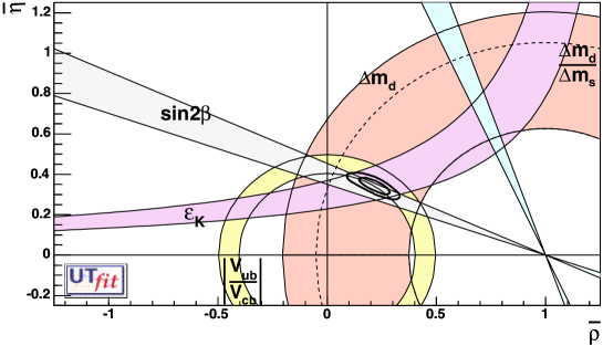
Figure 5: Correlations between other triangles

As I have said in the introduction: my goal was to “paint” a picture of the landscape of heavy-flavor hadrons and charged leptons and discuss correlations between them. Furthermore, charm hadrons and $\tau$ leptons act as gateways from light to heavy flavors.

First, I described this qualitatively:

• We have an even richer experimental landscape in charm & beauty hadrons and $\tau$ leptons for the future, as regards existing experiments at the LHCb (& perhaps the A Toroidal LHC Apparatus (ATLAS) & the Compact Muon Solenoid (CMS)), Beijing Spectrometer (BES) III, and Belle II. Their programs will deepen our understanding of fundamental dynamics. Plans are also in place for construction of the Super Tau-Charm Factory, Super-$Z^{0}$ Factory, etc.;

• It is not sufficient to measure two-body FS, as we must also probe three- & four-body FS. We must transition from the accuracy era to a precision-based period using the optimum tools (such as dispersion relations) that require a connection between theory & experiment;

• Searching for a golden medal is not enough. It is crucial to consider and measure correlations in flavor transitions;

• Using averaged strong phases is the first step. However, it is obvious that we must go beyond that and measure regional phases. The “road” towards three-body FS is obvious (in the world of theorists). For four-body FS, however, the landscape is more “complex”. First, we can probe averaged asymmetries, then moments (& correlations with different definitions), and then semi-regional asymmetries. Of course, appropriate thought should be applied.

Now I summarize the main points of this article semi-quantitatively:

(a) Flavor dynamics in the SM with three families of up- & down-quarks are described by six triangles, as shown in detail above. It is crucial to probe their correlations. There is a well-known example, namely, the “golden” triangle for $B$ transitions, with limits given by $\Delta M_{B_{d}}/\Delta M_{B_{s}}$ & $\epsilon_{K}$ (see Fig.5);

(b) While QCD is the only local QFT that can describe strong forces, it is crucial to understanding non-perturbative dynamics. We learn significantly more about its impact and its interaction with other tools, namely, OPE, HQE, & chiral symmetry. While charm hadrons primarily act as heavy-flavor particles, QCD tells us how they approach the limits of heavy-flavor states. In particular, charm transitions provide an excellent testing ground for our quantitative control of LQCD.

(c) QCD shows the differences between spectroscopy and weak dynamics, but also their connections, which are often subtle. Charm hadrons, including baryons, and $\tau$ particles provide very good testing grounds.

(d) We must transition from accuracy to precision as regards fundamental dynamics. We require not only additional data, but also additional & superior theoretical tools. Therefore, I have given an overview of these tools in Sect.2.

(e) Obviously, I support the probing of CP asymmetries. However, this is for good reasons. We probe interference between SM & ND amplitudes. More importantly, we must measure regional CP asymmetries with accuracy at the minimum [47, 77]. If a researcher does not like difficult challenges, she/he is in the wrong “business”.

Table 1 compares the oscillation parameter landscape for neutral mesons, which is already qualitatively rich. This landscape describes the transitions of the somewhat light-flavor meson $K^{0}$, heavy $B^{0}$ & $B^{0}_{s}$, and somewhat heavy $D^{0}$.

$K^{0}$	$D^{0}$	$B^{0}$	$B^{0}_{s}$
$\Delta M_{K}\simeq\bar{\Gamma}_{K}$	$\Delta M_{D}\ll\bar{\Gamma}_{D}$	$\Delta M_{B^{0}}\sim\bar{\Gamma}_{B^{0}}$	$\Delta M_{B^{0}_{s}}\gg\bar{\Gamma}_{B^{0}_{s}}$
$\Delta\Gamma_{K}\simeq 2\bar{\Gamma}_{K}$	$\Delta\Gamma_{D}\ll\bar{\Gamma}_{D}$	$\Delta\Gamma_{B^{0}}\ll\bar{\Gamma}_{B^{0}}$	$\Delta\Gamma_{B^{0}_{s}}\sim{\cal O}(\bar{\Gamma}_{B^{0}_{s}})$
$\Delta\Gamma_{K}\sim\Delta M_{K}$	$\Delta\Gamma_{D}\sim\Delta M_{D}$	$\Delta\Gamma_{B^{0}}\ll\Delta M_{B^{0}}$	$\Delta\Gamma_{B^{0}_{s}}\ll\Delta M_{B^{0}_{s}}$

As discussed in a long and detailed article [77], one can examine the plots of the mass distributions of $K_{S}$ vs. $K_{L}$ for $B_{d,L}$ vs. $B_{d,H}$ and $B_{s,L}$ vs. $B_{s,H}$ (on p. 1890–1891). The probing of quark flavor dynamics will remain important in the future, but the landscape has changed. In particular, we must transition from accuracy to precision, while also emphasizing correlations [78] .

Figure 6: Ludovisi throne: Goddess can be born with symmetry

Classical Greek art shows the connection between beauty and symmetry; an excellent example from Rome can be seen in Fig.6.

In the early Renaissance, approximately 1455 A.D., Piero della Francesa painted Constantine’s Dream, depicting the dream of Constantine (the Great) the night before his crucial battle on the fringes of Rome in 312 A.D. Here, the connection between different dimensions can be seen (see Fig.7).

Figure 7: Dreams

Piero della Francesa was also known as a mathematician & a geometer.

It is wonderful to dream about SUSY, etc., but we must be protected by data. However, in the long-term, surprising results can be obtained. Allow me to finish with a personal comment: for me, there should be a deeper, but subtle connection between fundamental dynamics and symmetry. The data are ultimately the judges, but research timescales can be long, as evidenced by our experience. I do not like to relinquish “wonderful” ideas at an early stage.

Acknowledgments: This work was supported by the NSF under grant number PHY-1215979. I am grateful to the Mainz Institute for Theoretical Physics (MITP) for its hospitality and its partial support during the completion of this work.

References

- [1] J. Bjorken, S. Glashow, Phys.Lett. 11 (1964) 255; Y. Hara, Phys.Rev. 134 (1964) B701; Z. Maki, Y. Ohuki, Prog.Theor.Phys. 32 (1964) 144.
- [2] S. Glashow, J. Illiopolous & L. Maiani, Phys.Rev. D2 (1970)1285.
- [3] K. Niu, E. Mikumo, Y. Maeda, Prog.Theor.Phys. 46 (1971) 1644.
- [4] L.B. Okun, Weak Interactions of Elementary Particles, Pergamon, 1965. The Russian original had appeared in 1963 – i.e., clearly before the discovery of CP violation.
- [5] A.C. Benvenuti et al., Phys.Rev.Lett. 34 (1975) 419.
- [6] M.K. Gaillard, B. Lee, Phys.Rev. D10 (1974) 897.
- [7] M.K. Gaillard, B. Lee, J. Rosner, Rev.Mod.Phys 47 (1975) 277..
- [8] T. Appelquist, H. D. Politzer, Phys.Rev.Lett. 34 (1975) 43.
- [9] I.I. Bigi et al., Phys.Lett. B181 (1986) 157.
- [10] ”Charm Physics”, edited by Ming-Han Ye & Tao Huang, CCAST (World Lab.), Symposion/Workshop Proceedings, Vol. 2, Gordon & Breach Science Publishers.
- [11] L. Wolfenstein, Phys.Rev.Lett. 13 (1964) 562.
- [12] M. Kobayashi, T. Maskawa, Prog.Theor.Phys. 49 (1973) 652.
- [13] S. Bianco et al., ”A Cicerone for the physics of charm”, Riv.Nuovo Cim.26N7(2003)1 [arXiv:hep-ex/0309021].
- [14] M.A. Shifman, M.B. Voloshin, Sov.Phys.JETP 64 (1986) 698.
- [15] A. Paul et al., Phys.Rev. D82 (2010) 094006 [arXiv:1008.3141]; A. Paul et al. Phys.Rev. D83 (2011) 114006 [arXiv:1101.6053]; A. Paul et al., Phys.Rev. D90 (2014) 0140035[arXiv:1212.4849[hep-ph]].
- [16] LHCb collab., R. Aaij et al., Phys.Rev.Lett. 111 (2013) 101801.
- [17] LHCb collab., R. Aaij et al., Phys.Rev.Lett. 112 (2014) 011801.
- [18] L. Wolfenstein, Phys.Rev.Lett. 51 (1983) 1945.
- [19] PDG, ”Particle Physics Booklet”, Chinese Physics C, Vol. 38, # 9 (Sept. 2014).
- [20] Y.H. Ahn, H-Y. Cheng, S. Oh, Phys.Lett. B703 (2011) 571; arXiv: 1106.0935.
- [21] I.I. Bigi, arXiv:1306.6014 [hep-ph], talk given at FPCP 2013.
- [22] S.L. Adler, Phys.Rev. 177 (1969) 2426; J.S. Bell, R. Jackiw, Nuovo Cimento 60 (1969) 47; W.A. Bardeen, Phys.Rev. 184 (1969) 1848.
- [23] J. Steinberger, Phys.Rev. 76 (1949) 1180.
- [24] I.I. Bigi, M. Shifman, N. Uraltsev, A. Vainshtein, Phys.Rev. D56 (1997) 4017; M. A. Shifman, “Quark-hadron duality,” Boris Ioffe Festschrift ’At the Frontier of Particle Physics / Handbook of QCD’, ed. M. Shifman (World Scientific, Singapore, 2001) [arXiv:hep-ph/0009131]; I.I. Bigi, N.G. Uraltsev, Int.J.Mod.Phys. A16 (2001) 5201-5248 [arXiv:hep-ph/0106346]; I.I. Bigi, Th. Mannel, arXiv:hep-ph/0212021.
- [25] I.I. Bigi, arXiv:1206.4554; it was meant to be part of a published paper in the future.
- [26] G. ’t Hooft, Nucl.Phys. B75 (1974)461; C. Callan, N. Coote, D. Gross, Phys.Rev. D13 (1976)1649; M. Einhorn, S. Nussinov, E. Rabinovici, Phys.Rev. D15 (1977)2282.
- [27] I.I. Bigi, in: Proceedings of Charm Physics, edited by Ming-Han Ye & Tao Huang, QCD161:S12:1987A, ps. 339 - 425 [in particular ps. 370 - 389]; SLAC-PUB-4349.
- [28] I.I. Bigi, V.A. Khoze, N.G. Uraltsev, A.I. Sanda, p. 175-248 in ”CP Violation”, C. Jarlskog (Editor), World Scientific (1988).
- [29] L. Wolfenstein, Phys.Rev. D43 (1991) 151.
- [30] I.I. Bigi, A.I. Sanda, ”CP Violation, Second Edition”, Cambridge Monographs on Particle Physics, Nuclear Physics and Cosmology (Cambridge University Press) 2009.
- [31] H.J. Lipkin, ”Lie Groups for Pedestrians ”, North-Holland Publ. Co., 1965.
- [32] M.R. Pennington, Proceed. of MESON2002, arXiv:hep-ph/0207220; J.R. Pelaez et al., Proceed. of the Hadron 2011 [arXiv:1109.2392]; J.R. Pelaez, arXiv:1301.4431 [hep-ph].
- [33] H. Lipkin, Phys.Lett. B621 (2005) 126; arXiv:hep-ph/0503022.
- [34] K. Wilson, Phys.Rev. 179 ((1969) 1499.
- [35] I.I. Bigi, N.G. Uraltsev, A.I. Vainshtein, Phys.Lett. B293 (1992) 430; Erratum-ibid. B297 (1993) 477.
- [36] I.I. Bigi, M. Shifman, N.G. Uraltsev, A.I. Vainshtein, Phys.Rev.Lett. 71 (1993) 496.
- [37] I.I. Bigi, M. Shifman, N.G. Uraltsev, A.I. Vainshtein, Phys.Rev. D50 (1994) 2234.
- [38] M. Voloshin, Phys.Rev. D46 (1992) 3062; M. Beneke, V. Braun, Nucl.Phys. B426 (1994) 301; N. Uraltsev, Int.J.Mod.Phys. A10 (1995) 515.
- [39] M.A. Shifman, A.I. Vainshtein, V.I. Zakharov, Nucl.Phys. B147 (1979) 385; 448.
- [40] I.I. Balitsky, V.M. Braun, A.V. Kolesnichenko, Nucl.Phys. B147 (1989) 509; V.I. Chernyak, I.R. Zhitnitsky, Nucl.Phys. B345 (1990) 137.
- [41] I. Bigi et al., Phys.Rev. D52 (1995) 196.
- [42] N. Uraltsev, Phys.Lett. B501 (2001) 86.
- [43] S. Turczyk, contrib. to Memorial Book for Kolya Uraltsev to be published in 2015.
- [44] Chr. Hanhart, Proceedings of CHARM 2013, ”Modelling low-mass resonances in multi-body decays” [arXiv:1311.6627]; B. Kubis, ”The role of final-state interactions in Dalitz plot studies” [arXiv:1108.5866]; S. Gardner, U.-G. Meissner, Phys.Rev. D65 (2002) 094004 [arXiv:hep-ph/0112281]; J. Donoghue, lecture given at the International School on Effective Field Theory [arXiv:hep-ph/9607351].
- [45] I. Bediaga et al.; Phys.Rev. D89 (2014) 074024 [arXiv:1401.3310 [hep-ph]]; I. Bediaga et al., Phys.Rev. D80 (2009) 096006 [arXiv:0905.4233]; I. Bediaga et al., Phys.Rev. D86 (2012) 036005 [arXiv:1205.3036].
- [46] M. Williams, Phys. Rev. D 84 (2011) 054015 [arXiv:1105.5338].
- [47] I.I. Bigi, Proceed. of KAON 2001, Pisa, 2001, 417 - 429 [arXiv:hep-ph/0107102].
- [48] A. Datta, D. London, Int.J.Mod. A19 (2004) 2505 [arXiv:hep-ph/0303159]; W. Bensalem, A. Datta, D. London, Phys.Rev. D66 (2002) 094004 [arXiv:hep-ph/0208054]; W. Bensalem, A. Datta, D. London, Phys.Lett. B538 (2002) 309.
- [49] G. Valencia, Phys.Rev. D39 (1989) 3339.
- [50] FOCUS Collab., Link, J.M. et al., Phys.Lett. B622 (2005) 239.
- [51] BaBar Collab., P. del Amo Sanchez et al., Phys. Rev. D81 (2010) 111103 [arXiv:1003.3397].
- [52] LHCb Collab., Roel Aaij et al., JHEP 1410 (2014) 005 [arXiv:1408.1299 [hep-ex]].
- [53] I.I. Bigi; TAU 2012 WS, Nuclear Physics B Proceedings Supplement (2013) 1 - 4 [arXiv:1210.2968; arXiv:1306.6014v2 [hep-ph]]; I.I. Bigi; arXiv:hep-ph/0012161, ”Rio de Janeiro 2000, Heavy quarks at fixed target”.
- [54] I.I. Bigi, Chinese Journal of Physics 45 # 3 (2007) 283 [arXiv:hep-ph/0703132].
- [55] L.M. Seghal, M. Wanninger, Phys.Rev. D46 (1992) 1035; 5209 (E); L.M. Seghal, J. van Leusen, Phys.Rev.Lett. 83 (1999) 4933; L.M. Seghal, J. van Leusen, Phys.Lett. B 489 (2000) 300.
- [56] C. Di Donato, G. Ricciardi, I.I. Bigi, Phys.Rev. D85 (2012) 013016 [arXiv:1105.3557].
- [57] S. Fajfer, P. Singer, J. Zupan, Phys.Rev. D64 (2001) 074008.
- [58] G. Burdman et al., Phys.Rev. D66 (2002) 014009.
- [59] R. Peccei, H. Quinn, Phys.Rev.Lett. 38 (1977) 1440; Phys.Rev. D16 (1977) 1791; R. D. Peccei, arXiv:hep-ph/0607268; C. Jarlskog (ed.), CP Violation, World Scientific, 1994.
- [60] G. Burdman et al., Phys.Rev. D52 (1995) 6383. S. Fajfer, hep-ph/0306263.
- [61] A. Lenz, contrib. to Memorial Book for Kolya Uraltsev to be published in 2015.
- [62] M. Golden, B. Grinstein, Phys. Lett. B 222 (1989) 501; I.I. Bigi, Proceedings of Tau-Charm Factory Workshop, Conf.Proc. C890523 (1989) 169-195.
- [63] M. Gronau, Phys.Lett. B730 (2014) 221; add.-ibid B735 (2014) 282.
- [64] R. Aaij et al., LHCb collab., arXiv:1410.4170v2 [hep-ex].
- [65] A. J. Bevan, B. T. Meadows, Phys. Rev. D 90 (2014) 094028 [arXiv:1310.0050].
- [66] A. Celis, V. Cirigliano, E. Passemar,Phys.Rev. D89 (2014) 095014 [arXiv:1403.5781[hep-ph]].
- [67] E. Passemar, I.I. Bigi, Hai-Bo Li, Cai-dian Lu, ”Higgs Factory as excellent ‘early’ Factory about Beauty, Charm Hadrons & Dynamics”, work in progress.
- [68] I.I. Bigi, A.I. Sanda, Phys. Lett. B 625 (2005) 47; I.I. Bigi, Nucl. Phys. B (Proc. Suppl.) 253–255 (2014) 91.
- [69] R.J. Sobie, Nucl. Phys. B (Proc. Suppl.) 253–255 (2014) 99.
- [70] W. Dekens et al., JHEP 1407 (2014) 069 [arXiv:1404.6082 [hep-ph]].
- [71] W. Bernreuther, O. Nachtmann, P. Overmann, Phys.Rev. D48 (1993) 78.
- [72] A. Pich, ”Precision Tau Physics”, Prog.Part.Nucl.Phys. 75 (2014) 41 [arXiv:1310.7922 [hep-ph]].
- [73] M. Fael, L. Mercolli, E. Passemar, Nucl. Phys.B (Proc. Suppl.)253–255(2014)103.
- [74] Belle Collab., K. Inami et al., Phys.Lett. B551 (2003) 16 [arXiv:hep-ex/0210066].
- [75] http://www.slac.stanford.edu/xorg/hfag/; Y. Amhis et al. [Heavy Flavor Averaging Group Collaboration], [arXiv:1207.1158 [hep-ex]].
- [76] ALEPH Collab., A. Heister et al., ”Search for anomalous weak dipole moments of the tau lepton”, Eur.Phys. J.C 30 (2003) 291 [arXiv:hep-ex/0209066].
- [77] I.I. Bigi, Rep.Prog.Phys. 70 (2007) 1869 - 1936.
- [78] I.I. Bigi, ”Flavour dynamics and CP violation in the SM: A tale in five parts of great successes, little understanding and promise for the future”, Riv.Nuovo Cim.30 (2007)1 - 93 [arXiv:hep-ph/0601167].