Fusion Probability in Dinuclear System

Abstract

Fusion can be described by the time evolution of a dinuclear system with two degrees of freedom, the relative motion and transfer of nucleons. In the presence of the coupling between two collective modes, we solve the Fokker-Planck equation in a locally harmonic approximation. The potential of a dinuclear system has the quasifission barrier and the inner fusion barrier, and the escape rates can be calculated by the Kramers’ model. To estimate the fusion probability, we calculate the quasifission rate and the fusion rate. We investigate the coupling effects on the fusion probability and the cross section of evaporation residue.

I Introduction

Fusion reaction has been greatly investigated, and superheavy elements have been synthesized in experiments. Many theoretical models describe heavy ion reaction and estimate the cross section of evaporation residue. Although much effort has been devoted to understanding fusion, it is still challenging to analyze and to predict data quantitativelyZagrebaev et al. (2001). Especially, the fusion probability is the least understood factor contributing to the cross section. The fusion probability has been studied as diffusion, and it is expected to be a logistic functionAdamian et al. (1997a); Swiatecki et al. (2005); Liu and Bao (2006). However, it might be sensitive to details of dynamics and be important for more quantitative analysis of data. In this work, we investigate the fusion probability by using the Fokker-Planck equation in the dinuclear system concept.

A dinuclear system consists of two colliding nuclei captured in an almost touching configurationVolkov (1978). In this concept, fusion can be understood as the time evolution of a dinuclear system. This description is different from other models in that it retains the individuality of nuclei and considers quasifission. A dinuclear system has two degrees of freedom, the relative motion and transfer of nucleons. To describe the relative motion, the internuclear distance $R$ is used as a collective coordinate. For transfer of nucleons, we define the mass asymmetry parameter

$$\eta=\frac{A_{1}-A_{2}}{A_{1}+A_{2}}\,,$$ (1)

where $A_{1}$ and $A_{2}$ are mass numbers of two nuclei. Each mode of motion is a diffusion process in a potential with an energy barrier. The escape rate over the barrier can be calculated by the Kramers’ model. There has been much research on the Kramers’ model (for a review and references, see Ref.Hanggi et al. (1990)). The extension of the model can be applied to fusion reaction.

The time evolution of a dinuclear system is described by the Fokker-Planck equation. For asymmetric reactions with not too high mass asymmetry, we have the following equationAdeev and Gonchar (1985); Adamian et al. (1997a):

$$\frac{\partial f}{\partial t} = -\mu_{R}p_{R}\frac{\partial f}{\partial R}-\mu_{\eta}p_{\eta}\frac{\partial f}{\partial\eta}-\left(\frac{\partial\mu_{R}}{\partial\eta}\frac{\mu_{\eta}}{\mu_{R}}p_{\eta}+\frac{\partial\mu_{\eta}}{\partial R}\frac{\mu_{R}}{\mu_{\eta}}p_{R}\right)f$$ (2)

$$+\left(\frac{\partial U}{\partial R}-\frac{\partial\mu_{R}}{\partial\eta}\frac{\mu_{\eta}}{\mu_{R}}p_{R}p_{\eta}+\frac{1}{2}\frac{\partial\mu_{\eta}}{\partial R}p_{\eta}^{2}\right)\frac{\partial f}{\partial p_{R}}+\left(\frac{\partial U}{\partial\eta}-\frac{\partial\mu_{\eta}}{\partial R}\frac{\mu_{R}}{\mu_{\eta}}p_{R}p_{\eta}+\frac{1}{2}\frac{\partial\mu_{R}}{\partial\eta}p_{R}^{2}\right)\frac{\partial f}{\partial p_{\eta}}$$

$$+\gamma_{R}\mu_{R}\frac{\partial(p_{R}f)}{\partial p_{R}}+\gamma_{\eta}\mu_{\eta}\frac{\partial(p_{\eta}f)}{\partial p_{\eta}}+D_{R}\frac{\partial^{2}f}{\partial p_{R}^{2}}+D_{\eta}\frac{\partial^{2}f}{\partial p_{\eta}^{2}}\,,$$

where $\mu_{i}$, $\gamma_{i}$, and $D_{i}$ ($i=R,\,\eta$) are the diagonal components of the inverse mass tensor, the friction tensor, and the diffusion tensor, respectively. By the fluctuation-dissipation theorem, $D_{i}=\gamma_{i}T_{i}$, where $T_{i}=(\hbar\omega_{i}/2)\,\mbox{coth}(\hbar\omega_{i}/2T)$ is the effective temperature with the energy of zero oscillations $\hbar\omega_{i}/2$ and the thermodynamic temperature $T=\sqrt{E^{*}/a}$ ($a=A/12\,\mbox{MeV}^{-1}$ is the level density parameter).

The Kramers’ problem described by Eq. (2) is useful in other quantum mechanical systems as well as a dinuclear system. The escape rate in two-dimensional potential has been calculatedLanger (1969); Weidenmuller and Jing-Shang (1984), but we use a different strategy to calculate the diffusion rates of two collective modes. By assuming that two modes are weakly coupled through the inverse mass tensors, we solve the Fokker-Planck equation perturbatively. We then calculate the quasifission rate and the fusion rate to estimate the fusion probability. Although we apply the rates to quasifission and fusion, our results for the diffusion rates can be applied to any escape problem in the presence of friction and diffusion.

In Section II, we review the Kramers’ model to calculate the escape rate. In Section III, we extend the model with two collective modes which are coupled through the inverse mass tensors. For weak coupling, we solve Eq. (2) perturbatively and calculate the diffusion rates of two modes. By applying the escape problem to a dinuclear system, we consider asymmetric fusion reactions in Section IV. We review the dinuclear system concept and estimate the coupling effects on the fusion probability and the cross section of evaporation residue. Finally, we summarize our results in Section V.

II Kramers’ Model

The fusion probability can be estimated by the Kramers’ model. Kramers considered the escape problem as a one-dimensional Brownian motion in a potential with deformation energyKramers (1940). In this section, we review the Kramers’ model, and the extension with two degrees of freedom will be discussed in the next section.

We consider a system initially at a local minimum $x=x_{a}$ (see Fig. 1). For moderate to high friction, the system can be excited enough to overcome the energy barrier at $x=x_{b}$ and go to the lower bound state at $x=x_{c}$. Since the energy barrier is supposed to be higher than the thermal energy ($E_{b}>T$), the escape process is slow. It can be understood as quasistationary diffusion.

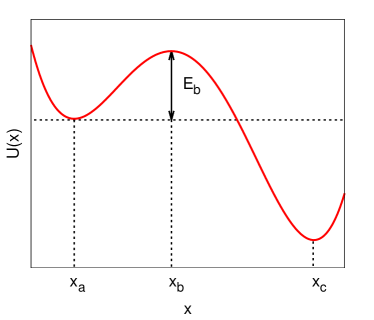
Figure 1: A schematic potential for the Kramers’ model. For moderate to high friction, a system at a local minimum $x=x_{a}$ can escape the energy barrier ($E_{b}>T$) at $x=x_{b}$ to go to the lower bound state at $x=x_{c}$.

The evolution of the system is described by the Fokker-Planck equationKramers (1940)

$$\left[\frac{\partial}{\partial t}+v\frac{\partial}{\partial x}-\mu\frac{dU(x)}{dx}\frac{\partial}{\partial v}\right]f(t,x,v)=\gamma\frac{\partial}{\partial v}\left[vf(t,x,v)+\mu T\frac{\partial f(t,x,v)}{\partial v}\right]\,.$$ (3)

In the diffusion limit, the system is in equilibrium everywhere except near the barrier at $x=x_{b}$. Thus, the dynamics may be evaluated by considering the potential around this point. In a locally harmonic approximation, the potential is given by $U(x)=-\omega_{b}^{2}(x-x_{b})^{2}/2\mu+U(x_{b})$, where $\omega_{b}$ is the angular frequency of the unstable state at the barrier. Around the barrier, there are neither sources nor sinks, and the distribution function satisfies the stationary Fokker-Planck equation.

In the stationary limit, we solve the Fokker-Planck equation by using a Maxwellian distribution

$$f(x,v)=\zeta(x,v)\,\exp\left[-\left(\frac{v^{2}}{2\mu}+U(x)\right)\Big{/}T\right]\,.$$ (4)

With the boundary conditions $\zeta(x_{a},v)=1$ and $\zeta(x_{c},v)=0$, the Kramers’ stationary solution isKramers (1940); Hanggi et al. (1990)

$$\zeta(x,v)=\frac{\omega_{b}^{2}}{\sqrt{2\pi\mu T\gamma\lambda}}\int_{(x-x_{b})-\lambda v/\omega_{b}^{2}}^{\infty}du\,\exp\left[-\frac{\omega_{b}^{4}u^{2}}{2\mu T\gamma\lambda}\right]\,,$$ (5)

where $\lambda=\sqrt{(\gamma/2)^{2}+\omega_{b}^{2}}-\gamma/2$. The stationary diffusion current is calculated by

$$\mathcal{J}(x_{b})=\int_{-\infty}^{\infty}dv\,vf(x_{b},v)\,,$$ (6)

and the number of particles at the initial state is

$$\mathcal{N}(x_{b})=\int_{-\infty}^{x_{b}}dx\int_{-\infty}^{\infty}dv\,f(x,v)\,,$$ (7)

where we use the locally harmonic potential $U(x)=\omega_{a}^{2}(x-x_{a})^{2}/2\mu+U(x_{a})$ around $x=x_{a}$. The escape rate is then given by the flux over populationKramers (1940)

$$\Gamma^{kr}=\frac{\mathcal{J}(x_{b})}{\mathcal{N}(x_{b})}=\frac{\lambda\omega_{a}}{2\pi\omega_{b}}\exp\left[-E_{b}/T\right]\,,$$ (8)

where the energy barrier is $E_{b}=U(x_{b})-U(x_{a})$.

The Kramers’ rate with the parabolic potential might give an upper bound of the escape ratePollak et al. (1990); Talkner (1995). For high friction, there can be recrossing over the energy barrier, and anharmonic corrections of the potential barrier reduce the escape rate. In Ref.Talkner (1995), the leading order effects of anharmonic potentials have been calculated perturbatively. In the next section, we use the same strategy to solve Eq. (2) in a locally harmonic approximation.

III Coupling through Inverse Mass Tensors

The Kramers’ quasistationary rate can be applied to two-dimensional potential of a dinuclear system. In general, the radial mode and the mass asymmetry mode are not separable, and they are coupled with each other. The coupling between two collective modes is weak for almost symmetric reactions, but it grows as the asymmetry increasesAdamian et al. (1995). For simplicity, we consider asymmetric dinuclear systems where the coupling between two modes is still weak. By following Ref.Talkner (1995) in which the Fokker-Planck equation is solved perturbatively, we investigate the coupling effects on the escape rates.

Similar to Eq. (4), we consider a distribution function of the form

$$f(R,\eta,v_{R},v_{\eta})=\zeta(R,\eta,v_{R},v_{\eta})\,\exp\left[-\left(v_{R}^{2}/2\mu_{R}T_{R}+v_{\eta}^{2}/2\mu_{\eta}T_{\eta}+U(R,\eta)/T_{eff}\right)\right]\,.$$ (9)

Around the barriers $(R=R_{b},\,\eta=\eta_{b})$, the two-dimensional potential is assumed to be

$$U(R,\eta)/T_{eff}=-\omega_{R_{b}}^{2}(R-R_{b})^{2}/2\mu_{R}T_{R}+U_{eff}(R_{b})/T_{R}\\ -\omega_{\eta_{b}}^{2}(\eta-\eta_{b})^{2}/2\mu_{\eta}T_{\eta}+U_{eff}(\eta_{b})/T_{\eta}\,,$$ (10)

where $U_{eff}(R_{b})$ and $U_{eff}(\eta_{b})$ are the effectively one-dimensional potentials in each collective coordinate. If there is no coupling through the inverse mass tensors, the escape rate is given by the Kramers’ rate in Eq. (8) for each degree of freedom. In that case, we have the zeroth order equation of motion

$$\mathcal{L}_{0}\,\zeta_{0}(R,\eta,v_{R},v_{\eta})=0\,,$$ (11)

where we have defined

$$\mathcal{L}_{0}=-v_{R}\frac{\partial}{\partial R}+\mu_{R}\frac{\partial U}{\partial R}\frac{\partial}{\partial v_{R}}-\gamma_{R}^{*}v_{R}\frac{\partial}{\partial v_{R}}+\mu_{R}\gamma_{R}^{*}T_{R}\frac{\partial^{2}}{\partial v_{R}^{2}}\\ -v_{\eta}\frac{\partial}{\partial\eta}+\mu_{\eta}\frac{\partial U}{\partial\eta}\frac{\partial}{\partial v_{\eta}}-\gamma_{\eta}^{*}v_{\eta}\frac{\partial}{\partial v_{\eta}}+\mu_{\eta}\gamma_{\eta}^{*}T_{\eta}\frac{\partial^{2}}{\partial v_{\eta}^{2}}\,,$$ (12)

with $\gamma_{i}^{*}=\mu_{i}\gamma_{i}$ ($i=R,\eta$). Since $R$ and $\eta$ modes are separable at the barriers, we have

$$\zeta_{0}(R,\eta,v_{R},v_{\eta})=\zeta_{R}(R,v_{R})\,\zeta_{\eta}(\eta,v_{\eta})\,,$$ (13)

and each factor is given by the Kramers’ stationary solution in Eq. (5):

$$\zeta_{R}(R,v_{R}) = \frac{\omega_{R_{b}}^{2}}{\sqrt{2\pi\mu_{R}T_{R}\gamma_{R}^{*}\lambda_{R}}}\int_{(R-R_{b})-\lambda_{R}v_{R}/\omega_{R_{b}}^{2}}^{\infty}du\,\exp\left[-\frac{\omega_{R_{b}}^{4}u^{2}}{2\mu_{R}T_{R}\gamma_{R}^{*}\lambda_{R}}\right]\,,$$

$$\zeta_{\eta}(\eta,v_{\eta}) = \frac{\omega_{\eta_{b}}^{2}}{\sqrt{2\pi\mu_{\eta}T_{\eta}\gamma_{\eta}^{*}\lambda_{\eta}}}\int_{(\eta-\eta_{b})-\lambda_{\eta}v_{\eta}/\omega_{\eta_{b}}^{2}}^{\infty}du\,\exp\left[-\frac{\omega_{\eta_{b}}^{4}u^{2}}{2\mu_{\eta}T_{\eta}\gamma_{\eta}^{*}\lambda_{\eta}}\right]\,,$$ (14)

where $\lambda_{i}=\sqrt{(\gamma_{i}^{*}/2)^{2}+\omega_{i_{b}}^{2}}-\gamma_{i}^{*}/2$ ($i=R,\eta$).

When the relative motion and the mass asymmetry are coupled by Eq. (2), we define the first order operator

$$\mathcal{L}_{1}=\left(-\frac{\partial\mu_{R}}{\partial\eta}\frac{1}{\mu_{R}}v_{R}v_{\eta}+\frac{1}{2}\frac{\partial\mu_{\eta}}{\partial R}\frac{\mu_{R}}{\mu_{\eta}^{2}}v_{\eta}^{2}\right)\frac{\partial}{\partial v_{R}}\\ +\left(-\frac{\partial\mu_{\eta}}{\partial R}\frac{1}{\mu_{\eta}}v_{R}v_{\eta}+\frac{1}{2}\frac{\partial\mu_{R}}{\partial\eta}\frac{\mu_{\eta}}{\mu_{R}^{2}}v_{R}^{2}\right)\frac{\partial}{\partial v_{\eta}}-\left(\frac{\partial\mu_{\eta}}{\partial R}\frac{1}{\mu_{\eta}}v_{R}+\frac{\partial\mu_{R}}{\partial\eta}\frac{1}{\mu_{R}}v_{\eta}\right)\,.$$ (15)

By expanding the solution in the order of coupling,

$$\zeta(R,\eta,v_{R},v_{\eta})=\zeta_{0}(R,\eta,v_{R},v_{\eta})+\zeta_{1}(R,\eta,v_{R},v_{\eta})+\zeta_{2}(R,\eta,v_{R},v_{\eta})+\cdots\,,$$ (16)

we have the equations of motionTalkner (1995):

$$-\mathcal{L}_{0}\zeta_{1}(R,\eta,v_{R},v_{\eta}) = \mathcal{L}_{1}\zeta_{0}(R,\eta,v_{R},v_{\eta})\,,$$ (17)

$$-\mathcal{L}_{0}\zeta_{2}(R,\eta,v_{R},v_{\eta}) = \mathcal{L}_{1}\zeta_{1}(R,\eta,v_{R},v_{\eta})\,,$$ (18)

and similarly for higher orders. In the following subsections, we will solve the first order equation of motion.

After solving for $\zeta_{1}(R,\eta,v_{R},v_{\eta})$, we need a strategy to calculate the escape rate in the two-dimensional potential. By noting that the zeroth order result should be two independent escape rates, we calculate the diffusion current and the number of particles as follows. For the relative motion, the current at the barrier is

$$\mathcal{J}_{R}(R_{b},\eta_{b})=\int_{-\infty}^{\infty}dv_{R}\int_{-\infty}^{\infty}dv_{\eta}\,v_{R}f(R_{b},\eta_{b},v_{R},v_{\eta})\,,$$ (19)

and the number of particles is defined as

$$\mathcal{N_{R}}(R_{b},\eta_{b})=\int_{-\infty}^{R_{b}}dR\int_{-\infty}^{\infty}dv_{R}\int_{-\infty}^{\infty}dv_{\eta}\,f(R,\eta_{b},v_{R},v_{\eta})\,,$$ (20)

where we have set $\eta=\eta_{b}$ to cancel $\exp[-U_{eff}(\eta_{b})/T_{\eta}]$ when taking the flux over population. Similarly for the mass asymmetry mode, we have

$$\mathcal{J}_{\eta}(R_{b},\eta_{b})=\int_{-\infty}^{\infty}dv_{R}\int_{-\infty}^{\infty}dv_{\eta}\,v_{\eta}f(R_{b},\eta_{b},v_{R},v_{\eta})\,,$$ (21)

and

$$\mathcal{N_{\eta}}(R_{b},\eta_{b})=\int_{-\infty}^{\infty}dv_{R}\int_{-\infty}^{\eta_{b}}d\eta\int_{-\infty}^{\infty}dv_{\eta}\,f(R_{b},\eta,v_{R},v_{\eta})\,.$$ (22)

Then the escape rates of two collective modes are given by the flux over population:

$$\Gamma_{R}=\frac{\mathcal{J}_{R}(R_{b},\eta_{b})}{\mathcal{N}_{R}(R_{b},\eta_{b})}\qquad\mbox{and}\qquad\Gamma_{\eta}=\frac{\mathcal{J}_{\eta}(R_{b},\eta_{b})}{\mathcal{N}_{\eta}(R_{b},\eta_{b})}\,.$$ (23)

Depending on reactions, not every term in Eq. (15) might be important to calculate the diffusion rates. To investigate the effect of each coupling, we solve the first order equation of motion separately. We present details in Section III.1, and only the results are presented in the following subsections.

III.1 $\mathcal{L}_{1}=-\frac{\partial\mu_{R}}{\partial\eta}\frac{1}{\mu_{R}}v_{R}v_{\eta}\frac{\partial}{\partial v_{R}}$

In this subsection, we assume $\mathcal{L}_{1}=-\frac{\partial\mu_{R}}{\partial\eta}\frac{1}{\mu_{R}}v_{R}v_{\eta}\frac{\partial}{\partial v_{R}}$. Since the right hand side of Eq. (17) is

$$\mathcal{L}_{1}\zeta_{0}(R,\eta,v_{R},v_{\eta})=-\frac{\partial\mu_{R}}{\partial\eta}\frac{1}{\mu_{R}}v_{R}v_{\eta}\frac{\partial\zeta_{R}(R,v_{R})}{\partial v_{R}}\,\zeta_{\eta}(\eta,v_{\eta})\,,$$ (24)

we expect the first order solution to be

$$\zeta_{1}(R,\eta,v_{R},v_{\eta})=\frac{\partial\mu_{R}}{\partial\eta}\frac{1}{\mu_{R}}\left[P_{1}(R,\eta,v_{R},v_{\eta})\frac{\partial\zeta_{R}(R,v_{R})}{\partial v_{R}}\zeta_{\eta}(\eta,v_{\eta})\right.\\ \left.+P_{2}(R,\eta,v_{R},v_{\eta})\frac{\partial\zeta_{R}(R,v_{R})}{\partial v_{R}}\frac{\partial\zeta_{\eta}(\eta,v_{\eta})}{\partial v_{\eta}}\right]\,,$$ (25)

where $P_{i}(R,\eta,v_{R},v_{\eta})$ ($i=1,\,2$) is a polynomial of collective coordinates and velocities. By plugging Eq. (25) into Eq. (17), we have

$$\left[v_{R}\frac{\partial}{\partial R}-\omega_{R_{b}}^{2}(R-R_{b})\frac{\partial}{\partial v_{R}}+(2\lambda_{R}+\gamma_{R}^{*})v_{R}\frac{\partial}{\partial v_{R}}-\mu_{R}\gamma_{R}^{*}T_{R}\frac{\partial^{2}}{\partial v_{R}^{2}}+\lambda_{R}\right.\\ \left.+v_{\eta}\frac{\partial}{\partial\eta}+\omega_{\eta_{b}}^{2}(\eta-\eta_{b})\frac{\partial}{\partial v_{\eta}}+\gamma_{\eta}^{*}v_{\eta}\frac{\partial}{\partial v_{\eta}}-\mu_{\eta}\gamma_{\eta}^{*}T_{\eta}\frac{\partial^{2}}{\partial v_{\eta}^{2}}\right]P_{1}(R,\eta,v_{R},v_{\eta})=-v_{R}v_{\eta}\,,$$ (26)

and

$$\left[v_{R}\frac{\partial}{\partial R}-\omega_{R_{b}}^{2}(R-R_{b})\frac{\partial}{\partial v_{R}}+(2\lambda_{R}+\gamma_{R}^{*})v_{R}\frac{\partial}{\partial v_{R}}-\mu_{R}\gamma_{R}^{*}T_{R}\frac{\partial^{2}}{\partial v_{R}^{2}}+\lambda_{R}\right.\\ \left.+v_{\eta}\frac{\partial}{\partial\eta}-\omega_{\eta_{b}}^{2}(\eta-\eta_{b})\frac{\partial}{\partial v_{\eta}}+(2\lambda_{\eta}+\gamma_{\eta}^{*})v_{\eta}\frac{\partial}{\partial v_{\eta}}-\mu_{\eta}\gamma_{\eta}^{*}T_{\eta}\frac{\partial^{2}}{\partial v_{\eta}^{2}}+\lambda_{\eta}\right]P_{2}(R,\eta,v_{R},v_{\eta})\\ =2\mu_{\eta}\gamma_{\eta}^{*}T_{\eta}\frac{\partial P_{1}(R,\eta,v_{R},v_{\eta})}{\partial v_{\eta}}\,.$$ (27)

The polynomials are found to be

$$P_{1}(R,\eta,v_{R},v_{\eta}) = a_{1}(R-R_{b})(\eta-\eta_{b})+a_{2}(R-R_{b})v_{\eta}+a_{3}(\eta-\eta_{b})v_{R}+a_{4}v_{R}v_{\eta}\,,\,\,$$

$$P_{2}(R,\eta,v_{R},v_{\eta}) = a_{5}(R-R_{b})+a_{6}v_{R}\,,$$ (28)

where $a_{i}$ $(i=1,\cdots,6)$ is a constant. It is straightforward to determine the constants:

$$a_{1} = \frac{\omega_{\eta_{b}}^{2}\omega_{R_{b}}^{2}(\gamma_{\eta}^{*}+\gamma_{R}^{*}+4\lambda_{R})a_{4}}{\lambda_{R}(3\lambda_{\eta}^{2}-4\lambda_{R}^{2})+\gamma_{\eta}^{*}[\gamma_{R}^{*}(\lambda_{\eta}-2\lambda_{R})+\lambda_{R}(3\lambda_{\eta}-4\lambda_{R})]+\gamma_{R}^{*}(\lambda_{\eta}^{2}-2\lambda_{R}^{2})}\,,$$

$$a_{2} = \frac{\omega_{R_{b}}^{2}(\gamma_{R}^{*}\lambda_{R}+3\lambda_{R}^{2}+\omega_{\eta_{b}}^{2}+\omega_{R_{b}}^{2})a_{4}}{\gamma_{R}^{*}(2\lambda_{R}^{2}-\lambda_{\eta}^{2})+\lambda_{R}(4\lambda_{R}^{2}-3\lambda_{\eta}^{2})+\gamma_{\eta}^{*}[\gamma_{R}^{*}(2\lambda_{R}-\lambda_{\eta})+\lambda_{R}(4\lambda_{R}-3\lambda_{\eta})]}\,,$$

$$a_{3} = -\frac{\omega_{\eta_{b}}^{2}[\lambda_{\eta}^{2}+\gamma_{\eta}^{*}(\lambda_{\eta}-\lambda_{R})+\gamma_{R}^{*}\lambda_{R}]a_{4}}{\lambda_{R}(3\lambda_{\eta}^{2}-4\lambda_{R}^{2})+\gamma_{\eta}^{*}[\gamma_{R}^{*}(\lambda_{\eta}-2\lambda_{R})+\lambda_{R}(3\lambda_{\eta}-4\lambda_{R})]+\gamma_{R}^{*}(\lambda_{\eta}^{2}-2\lambda_{R}^{2})}\,,$$

$$a_{4} = -\frac{\lambda_{\eta}^{2}\lambda_{R}[\lambda_{R}(3\lambda_{\eta}^{2}-4\lambda_{R}^{2})+\gamma_{\eta}^{*}\{\gamma_{R}^{*}(\lambda_{\eta}-2\lambda_{R})+\lambda_{R}(3\lambda_{\eta}-4\lambda_{R})\}+\gamma_{R}^{*}(\lambda_{\eta}^{2}-2\lambda_{R}^{2})]}{(\lambda_{\eta}-2\lambda_{R})(2\lambda_{R}-\lambda_{\eta}+\gamma_{R}^{*})(2\lambda_{\eta}\lambda_{R}+\omega_{\eta_{b}}^{2})[\lambda_{R}\omega_{\eta_{b}}^{2}+\lambda_{\eta}(\lambda_{R}^{2}+\omega_{R_{b}}^{2})]}\,,$$

$$a_{5} = \frac{2\gamma_{\eta}^{*}\mu_{\eta}T_{\eta}[(\gamma_{R}^{*}+\lambda_{\eta}+3\lambda_{R})a_{2}+\omega_{R_{b}}^{2}a_{4}]}{\lambda_{\eta}^{2}+4\lambda_{\eta}\lambda_{R}+3\lambda_{R}^{2}+\gamma_{R}^{*}(\lambda_{\eta}+\lambda_{R})+\omega_{R_{b}}^{2}}\,,$$

$$a_{6} = \frac{2\gamma_{\eta}^{*}\mu_{\eta}T_{\eta}[-a_{2}+(\lambda_{\eta}+\lambda_{R})a_{4}]}{(\lambda_{\eta}+\lambda_{R})(\gamma_{R}^{*}+\lambda_{\eta}+3\lambda_{R})+\omega_{R_{b}}^{2}}\,.$$ (29)

By using Eqs.(19) and (20), we find the diffusion current and the number of particles for the relative motion to be

$$\mathcal{J}_{R}(R_{b},\eta_{b}) = \sqrt{\frac{\pi\mu_{\eta}T_{\eta}}{2}}\frac{\mu_{R}T_{R}\lambda_{R}}{\omega_{R_{b}}}\left[1+\frac{\partial\mu_{R}}{\partial\eta}\frac{1}{\mu_{R}}\left(a_{4}\mu_{\eta}T_{\eta}+a_{6}\right)\sqrt{\frac{2}{\pi\mu_{\eta}T_{\eta}}}\frac{\gamma_{R}^{*}\lambda_{R}\lambda_{\eta}}{\omega_{R_{b}}^{2}\omega_{\eta_{b}}}\right]$$

$$\qquad\times\bigg{.}\bigg{.}\exp\left[-U_{eff}(R_{b})/T_{R}-U_{eff}(\eta_{b})/T_{\eta}\right]\,,$$

$$\mathcal{N}_{R}(R_{b},\eta_{b}) = \sqrt{2\pi\mu_{\eta}T_{\eta}}\frac{\pi\mu_{R}T_{R}}{\omega_{R_{a}}}\,\exp\left[-U_{eff}(R_{a})/T_{R}-U_{eff}(\eta_{b})/T_{\eta}\right]\,.$$ (30)

Then the flux over population is used to determine the escape rate

$$\Gamma_{R}=\Gamma_{R}^{kr}\left[1+\frac{\partial\mu_{R}}{\partial\eta}\frac{1}{\mu_{R}}\left(a_{4}\mu_{\eta}T_{\eta}+a_{6}\right)\sqrt{\frac{2}{\pi\mu_{\eta}T_{\eta}}}\frac{\gamma_{R}^{*}\lambda_{R}\lambda_{\eta}}{\omega_{R_{b}}^{2}\omega_{\eta_{b}}}\right]\,,$$ (31)

where we have used the Kramers’ escape rate in Eq. (8). Similarly for the mass asymmetry mode, we have

$$\mathcal{J}_{\eta}(R_{b},\eta_{b}) = \sqrt{\frac{\pi\mu_{R}T_{R}}{2}}\frac{\mu_{\eta}T_{\eta}\lambda_{\eta}}{\omega_{\eta_{b}}}\,\exp\left[-U_{eff}(R_{b})/T_{R}-U_{eff}(\eta_{b})/T_{\eta}\right]\,,$$

$$\mathcal{N}_{\eta}(R_{b},\eta_{b}) = \sqrt{2\pi\mu_{R}T_{R}}\frac{\pi\mu_{\eta}T_{\eta}}{\omega_{\eta_{a}}}\,\exp\left[-U_{eff}(R_{b})/T_{R}-U_{eff}(\eta_{a})/T_{\eta}\right]\,,$$ (32)

and the diffusion rate is

$$\Gamma_{\eta}=\Gamma_{\eta}^{kr}\,.$$ (33)

We note that the escape rate of the $R$ mode changes by the coupling, while the $\eta$ mode is not affected. The coupling effects depend on the friction coefficients and the angular frequencies at the barriers.

III.2 $\mathcal{L}_{1}=\frac{1}{2}\frac{\partial\mu_{\eta}}{\partial R}\frac{\mu_{R}}{\mu_{\eta}^{2}}v_{\eta}^{2}\frac{\partial}{\partial v_{R}}$

The first order solution is of the form

$$\zeta_{1}(R,\eta,v_{R},v_{\eta})=\frac{1}{2}\frac{\partial\mu_{\eta}}{\partial R}\frac{\mu_{R}}{\mu_{\eta}^{2}}\left[P_{1}(R,\eta,v_{R},v_{\eta})\frac{\partial\zeta_{R}(R,v_{R})}{\partial v_{R}}\zeta_{\eta}(\eta,v_{\eta})\right.\\ \left.+P_{2}(R,\eta,v_{R},v_{\eta})\frac{\partial\zeta_{R}(R,v_{R})}{\partial v_{R}}\frac{\partial\zeta_{\eta}(\eta,v_{\eta})}{\partial v_{\eta}}\right]\,,$$ (34)

and the polynomials are found to be

$$P_{1}(R,\eta,v_{R},v_{\eta}) = b_{1}+b_{2}(\eta-\eta_{b})^{2}+b_{3}(\eta-\eta_{b})v_{\eta}+b_{4}v_{\eta}^{2}\,,$$

$$P_{2}(R,\eta,v_{R},v_{\eta}) = b_{5}(\eta-\eta_{b})+b_{6}v_{\eta}\,,$$ (35)

where the constants are

$$b_{1} = \frac{2\mu_{\eta}\gamma_{\eta}^{*}T_{\eta}b_{4}}{\lambda_{R}}\,,$$

$$b_{2} = \frac{2\omega_{\eta_{b}}^{4}b_{4}}{(\lambda_{R}^{2}-2\lambda_{\eta}^{2})+\gamma_{\eta}^{*}(\lambda_{R}-2\lambda_{\eta})}\,,$$

$$b_{3} = -\frac{2\lambda_{R}\omega_{\eta_{b}}^{2}b_{4}}{(\lambda_{R}^{2}-2\lambda_{\eta}^{2})+\gamma_{\eta}^{*}(\lambda_{R}-2\lambda_{\eta})}\,,$$

$$b_{4} = \frac{(\lambda_{R}^{2}-2\lambda_{\eta}^{2})+\gamma_{\eta}^{*}(\lambda_{R}-2\lambda_{\eta})}{(\gamma_{\eta}^{*}+\lambda_{R})(\lambda_{R}-2\lambda_{\eta})(2\gamma_{\eta}^{*}+\lambda_{R}+2\lambda_{\eta})}\,,$$

$$b_{5} = \frac{2\mu_{\eta}\gamma_{\eta}^{*}T_{\eta}[(\gamma_{\eta}^{*}+\lambda_{R}+3\lambda_{\eta})b_{3}+2\omega_{\eta_{b}}^{2}b_{4}]}{\lambda_{R}^{2}+4\lambda_{R}\lambda_{\eta}+3\lambda_{\eta}^{2}+\gamma_{\eta}^{*}(\lambda_{R}+\lambda_{\eta})+\omega_{\eta_{b}}^{2}}\,,$$

$$b_{6} = \frac{2\mu_{\eta}\gamma_{\eta}^{*}T_{\eta}[-b_{3}+2(\lambda_{R}+\lambda_{\eta})b_{4}]}{(\lambda_{R}+\lambda_{\eta})(\gamma_{\eta}^{*}+\lambda_{R}+3\lambda_{\eta})+\omega_{\eta_{b}}^{2}}\,.$$ (36)

The escape rates of two collective modes are

$$\Gamma_{R} = \Gamma_{R}^{kr}\,,$$ (37)

$$\Gamma_{\eta} = \Gamma_{\eta}^{kr}\left[1+\frac{\partial\mu_{\eta}}{\partial R}\frac{1}{\mu_{\eta}^{2}}\sqrt{\frac{\mu_{R}}{2\pi T_{R}}}\frac{\lambda_{R}}{\omega_{R_{b}}}\bigg{\{}b_{1}+b_{4}\mu_{\eta}T_{\eta}\left(2+\frac{\gamma_{\eta}^{*}\lambda_{\eta}}{\omega_{\eta_{b}}^{2}}\right)+b_{6}\frac{\gamma_{\eta}^{*}\lambda_{\eta}}{\omega_{\eta_{b}}^{2}}\bigg{\}}\right]\,.$$ (38)

In this case, the diffusion rate of the $\eta$ mode is affected by the coupling.

III.3 $\mathcal{L}_{1}=-\frac{\partial\mu_{\eta}}{\partial R}\frac{1}{\mu_{\eta}}v_{R}v_{\eta}\frac{\partial}{\partial v_{\eta}}$

This case is similar to Section III.1 by interchanging $(R,v_{R})$ and $(\eta,v_{\eta})$. The first order solution has the form

$$\zeta_{1}(R,\eta,v_{R},v_{\eta})=\frac{\partial\mu_{\eta}}{\partial R}\frac{1}{\mu_{\eta}}\left[P_{1}(R,\eta,v_{R},v_{\eta})\zeta_{R}(R,v_{R})\frac{\partial\zeta_{\eta}(\eta,v_{\eta})}{\partial v_{\eta}}\right.\\ \left.+P_{2}(R,\eta,v_{R},v_{\eta})\frac{\partial\zeta_{R}(R,v_{R})}{\partial v_{R}}\frac{\partial\zeta_{\eta}(\eta,v_{\eta})}{\partial v_{\eta}}\right]\,,$$ (39)

where the polynomials are

$$P_{1}(R,\eta,v_{R},v_{\eta}) = c_{1}(R-R_{b})(\eta-\eta_{b})+c_{2}(\eta-\eta_{b})v_{R}+c_{3}(R-R_{b})v_{\eta}+c_{4}v_{R}v_{\eta}\,,$$

$$P_{2}(R,\eta,v_{R},v_{\eta}) = c_{5}(\eta-\eta_{b})+c_{6}v_{\eta}\,.$$ (40)

The constant $c_{i}$ ($i=1,\cdots,6$) is given by Eq. (III.1) except that $(\gamma_{R}^{*},\,\lambda_{R},\,\omega_{R_{b}},\mu_{R},T_{R})$ and $(\gamma_{\eta}^{*},\,\lambda_{\eta},\,\omega_{\eta_{b}},\mu_{\eta},T_{\eta})$ interchange. The escape rates of two collective modes are

$$\Gamma_{R} = \Gamma_{R}^{kr}\,,$$ (41)

$$\Gamma_{\eta} = \Gamma_{\eta}^{kr}\left[1+\frac{\partial\mu_{\eta}}{\partial R}\frac{1}{\mu_{\eta}}\left(c_{4}\mu_{R}T_{R}+c_{6}\right)\sqrt{\frac{2}{\pi\mu_{R}T_{R}}}\frac{\lambda_{R}\lambda_{\eta}\gamma_{\eta}^{*}}{\omega_{R_{b}}\omega_{\eta_{b}}^{2}}\right]\,.$$ (42)

III.4 $\mathcal{L}_{1}=\frac{1}{2}\frac{\partial\mu_{R}}{\partial\eta}\frac{\mu_{\eta}}{\mu_{R}^{2}}v_{R}^{2}\frac{\partial}{\partial v_{\eta}}$

This case is similar to Section III.2 by interchanging $(R,v_{R})$ and $(\eta,v_{\eta})$. The first order solution is of the form

$$\zeta_{1}(R,\eta,v_{R},v_{\eta})=\frac{1}{2}\frac{\partial\mu_{R}}{\partial\eta}\frac{\mu_{\eta}}{\mu_{R}^{2}}\left[P_{1}(R,\eta,v_{R},v_{\eta})\zeta_{R}(R,v_{R})\frac{\partial\zeta_{\eta}(\eta,v_{\eta})}{\partial v_{\eta}}\right.\\ \left.+P_{2}(R,\eta,v_{R},v_{\eta})\frac{\partial\zeta_{R}(R,v_{R})}{\partial v_{R}}\frac{\partial\zeta_{\eta}(\eta,v_{\eta})}{\partial v_{\eta}}\right]\,,$$ (43)

with the polynomials

$$P_{1}(R,\eta,v_{R},v_{\eta}) = d_{1}+d_{2}(R-R_{b})^{2}+d_{3}(R-R_{b})v_{R}+d_{4}v_{R}^{2}\,,$$

$$P_{2}(R,\eta,v_{R},v_{\eta}) = d_{5}(R-R_{b})+d_{6}v_{R}\,.$$ (44)

The constant $d_{i}$ ($i=1,\cdots,6$) is given by Eq. (III.2) except that $(\gamma_{R}^{*},\,\lambda_{R},\,\omega_{R_{b}},\mu_{R},T_{R})$ and $(\gamma_{\eta}^{*},\,\lambda_{\eta},\,\omega_{\eta_{b}},\mu_{\eta},T_{\eta})$ interchange. The escape rates of two collective modes are

$$\Gamma_{R} = \Gamma_{R}^{kr}\left[1+\frac{\partial\mu_{R}}{\partial\eta}\frac{1}{\mu_{R}^{2}}\sqrt{\frac{\mu_{\eta}}{2\pi T_{\eta}}}\frac{\lambda_{\eta}}{\omega_{\eta_{b}}}\bigg{\{}d_{1}+d_{4}\mu_{R}T_{R}\left(2+\frac{\gamma_{R}^{*}\lambda_{R}}{\omega_{R_{b}}^{2}}\right)+d_{6}\frac{\gamma_{R}^{*}\lambda_{R}}{\omega_{R_{b}}^{2}}\bigg{\}}\right]\,,$$ (45)

$$\Gamma_{\eta} = \Gamma_{\eta}^{kr}\,.$$ (46)

III.5 $\mathcal{L}_{1}=-\frac{\partial\mu_{\eta}}{\partial R}\frac{1}{\mu_{\eta}}v_{R}$ or $\mathcal{L}_{1}=-\frac{\partial\mu_{R}}{\partial\eta}\frac{1}{\mu_{R}}v_{\eta}$

We assume $\mathcal{L}_{1}=-\frac{\partial\mu_{\eta}}{\partial R}\frac{1}{\mu_{\eta}}v_{R}$. The first order solution is

$$\zeta_{1}(R,\eta,v_{R},v_{\eta})=\frac{\partial\mu_{\eta}}{\partial R}\frac{1}{\mu_{\eta}}P(R,\eta,v_{R},v_{\eta})\,\zeta_{R}(R,v_{R})\,\zeta_{\eta}(\eta,v_{\eta})\,,$$ (47)

where the polynomial is found to be $P(R,\eta,v_{R},v_{\eta})=-(R-R_{b})+c$. For a constant $c=0$, this coupling does not change the diffusion rates of two modes.

Similarly, the coupling $\mathcal{L}_{1}=-\frac{\partial\mu_{R}}{\partial\eta}\frac{1}{\mu_{R}}v_{\eta}$ does not affect the escape rates.

III.6 Coupling Effects on Escape Rates

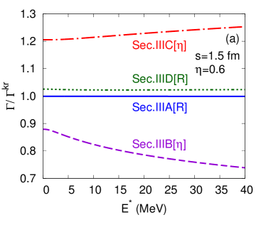
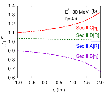
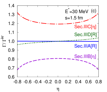
Figure 2: The ratios of the escape rate to the Kramers’ rate (a) as a function of the excitation energy for $s=1.5\,\mbox{fm}$ and $\eta=0.6$, (b) as a function of the distance for $E^{*}=30\,\mbox{MeV}$ and $\eta=0.6$, and (c) as a function of the mass asymmetry parameter for $E^{*}=30\,\mbox{MeV}$ and $s=1.5\,\mbox{fm}$. The blue solid lines are for the quasifission rate of Eq. (31) in Section III.1, the violet dashed lines are for the fusion rate of Eq. (38) in Section III.2, the red dashed-dotted lines are for the fusion rate of Eq. (42) in Section III.3, and the green dotted lines are for the quasifission rate of Eq. (45) in Section III.4. The parameters of $\hbar\omega_{R_{b}}=2\,\mbox{MeV}$, $\hbar\omega_{\eta_{b}}=1\,\mbox{MeV}$, $\hbar\gamma_{R}^{*}=\hbar\gamma_{\eta}^{*}=2\,\mbox{MeV}$, and $A=300$ are used.

As seen in Eqs. (31), (38), (42), and (45), the escape rates are affected by the coupling between two collective modes. The coupling effects generally depend on the friction coefficients $(\gamma_{R}^{*},\gamma_{\eta}^{*})$ and the angular frequencies $(\omega_{R_{b}},\omega_{\eta_{b}})$. In this subsection, we investigate the degree of the coupling effects on the escape rates, by using specific parameters. For a dinuclear system, the diffusion rates of the $R$ and $\eta$ modes are interpreted as the quasifission rate and the fusion rate, respectively (see Section IV).

The inverse mass tensors of a dinuclear system are given byAdamian et al. (1997a, 1995, 2014)

$$\mu_{R} = \frac{4}{Am}\frac{1}{1-\eta^{2}}\left(1-\frac{\nu}{1-\eta^{2}}\right)\qquad\mbox{with}\qquad\nu=\frac{1}{A}(\xi_{0}-\xi_{1}\eta^{2})(1-\xi s)\,,$$

$$\mu_{\eta} = \frac{1}{Am}\frac{\nu}{2\sqrt{2\pi}b^{2}}\,,$$ (48)

where $m$ is the nucleon mass, $s=R-R_{1}-R_{2}$, $\xi_{0}=16$, $\xi_{1}=17.5$, $\xi=0.3\,\mbox{fm}^{-1}$, and $b=1\,\mbox{fm}$. For a dinuclear system with $A=300$, we use the coefficients of $\hbar\omega_{R_{b}}=2\,\mbox{MeV}$, $\hbar\omega_{\eta_{b}}=1\,\mbox{MeV}$, and $\hbar\gamma_{R}^{*}=\hbar\gamma_{\eta}^{*}=2\,\mbox{MeV}$.

In Fig. 2, we present the ratios of the escape rate to the Kramers’ rate. The blue solid lines are for the quasifission rate of Eq. (31) in Section III.1, the violet dashed lines are for the fusion rate of Eq. (38) in Section III.2, the red dashed-dotted lines are for the fusion rate of Eq. (42) in Section III.3, and the green dotted lines are for the quasifission rate of Eq. (45) in Section III.4. Fig. 2 (a) shows the coupling effects depending on the excitation energy for $s=1.5\,\mbox{fm}$ and $\eta=0.6$. For the particular choice of parameters, the fusion rate in Section III.2 decreases by $10\,$-$\,25\%$. On the other hand, the coupling in Section III.3 increases the fusion rate by $20\,$-$\,25\%$. Thus, in the presence of both couplings, there might be cancellation in some of the effects. For the quasifission rate, the coupling effects are relatively low. The coupling in Section III.4 increases the rate by $2.5\%$, and the effect in Section III.1 is less than $1\%$. Fig. 2 (b) shows the coupling effects depending on the distance for $E^{*}=30\,\mbox{MeV}$ and $\eta=0.6$. As the distance increases, the effects on the fusion rate grow due to the increasing mass of the $\eta$ mode. The fusion rates change by $10\,$-$\,30\%$ while the quasifission rates are not affected much. The couplings effects also depend on the mass asymmetry as in Fig. 2 (c). Dinuclear systems with higher mass asymmetry are affected more by the coupling through the inverse mass tensors.

IV Dinuclear System

In this section, we review the dinuclear system concept by following Refs.Adamian et al. (1997a); Antonenko et al. (1995); Adamian et al. (1997b, 1998) and apply the Kramers’ escape problem to a dinuclear system. We discuss the diabatic nucleus-nucleus potential and the driving potential. By the Kramers’ model, quasifission and fusion are described as diffusion in two collective coordinates. The cross section of evaporation residue is determined by estimating the fusion probability and the survival probability. Based on the study in the previous section, we discuss the coupling effects on the fusion probability and the cross section.

IV.1 Diabatic Potential

The diabatic nucleus-nucleus potential consists of the Coulomb potential, the nuclear potential, and the centrifugal potential:

$$V(R,J)=V_{C}(R)+V_{N}(R)+V_{rot}(R,J)\,,$$ (49)

where $J$ is the angular momentum. We consider axially symmetric systems described by $R_{i}(\theta_{i})=R_{0i}\left[1+\beta_{i}Y_{20}(\theta_{i})\right]$, where $\beta_{i}$ is the quadrupole deformation parameter and $R_{0i}=r_{0}A_{i}^{1/3}$ with $r_{0}=1.16\,\mbox{fm}$. Then the Coulomb potential is given byWong (1973)

$$V_{C}(R)=\frac{e^{2}Z_{1}Z_{2}}{R}+\frac{3}{5}\frac{e^{2}Z_{1}Z_{2}}{R^{3}}\sum_{i=1,2}R_{0i}^{2}\beta_{i}Y_{20}(\theta_{i})\,.$$ (50)

The centrifugal potential is

$$V_{rot}(R,J)=\frac{\hbar^{2}J(J+1)}{2\mathcal{I}}\,,$$ (51)

where $\mathcal{I}$ is the moment of inertia.

The nuclear potential in the double folding form is

$$V_{N}(R)=\int d{\bm{r}}_{1}\int d{\bm{r}}_{2}\,\rho_{1}({\bm{r}}_{1})\,\rho_{2}(\bm{R}-{\bm{r}}_{2})\,F({\bm{r}}_{1}-{\bm{r}}_{2})\,,$$ (52)

where $F({\bm{r}}_{1}-{\bm{r}}_{2})$ is the nucleon-nucleon interaction. A well-known ansatz for the density dependent interaction givesMigdal (1967)

$$F({\bm{r}}_{1}-{\bm{r}}_{2})=C_{0}\left[F_{in}\frac{\rho({\bm{r}}_{1})}{\rho_{0}}+F_{ex}\left(1-\frac{\rho({\bm{r}}_{1})}{\rho_{0}}\right)\right]\delta({\bm{r}}_{1}-{\bm{r}}_{2})\,,$$ (53)

where

$$F_{in}=f_{in}+f_{in}^{\prime}\frac{N_{1}-Z_{1}}{A_{1}}\frac{N_{2}-Z_{2}}{A_{2}}\,,$$ (54)

and similarly for $F_{ex}$. The density $\rho({\bm{r}})=\rho_{1}({\bm{r}})+\rho_{2}({\bm{r}})$ is given by the Wood-Saxon form

$$\rho_{i}({\bm{r}})=\frac{\rho_{0}}{1+\exp[(r-R_{i}(\theta_{i}))/a_{0}]}\,.$$ (55)

We use the parameters of $C_{0}=300\,\mbox{MeV}\,\mbox{fm}^{3}$, $f_{in}=0.09$, $f_{in}^{\prime}=0.42$, $f_{ex}=-2.59$, $f_{ex}^{\prime}=0.54$, $\rho_{0}=0.17\,\mbox{fm}^{-3}$, and $a_{0}=0.55\,\mbox{fm}$.

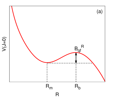
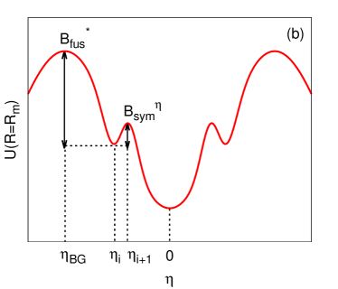
Figure 3: (a) The diabatic nucleus-nucleus potential has an energy barrier, $B_{qf}^{R}=V(R_{b})-V(R_{m})$. (b) The driving potential has the inner fusion barrier, $B_{fus}^{*}=U(\eta_{BG})-U(\eta_{i})$. There is another barrier for symmetrization of a dinuclear system, $B_{sym}^{\eta}=U(\eta_{i+1})-U(\eta_{i})$. The quasifission barrier is defined as $B_{qf}=\mbox{Min}[B_{qf}^{R},B_{sym}^{\eta}]$.

For $J=0$, a schematic nucleus-nucleus potential is shown in Fig. 3 (a). In contrast to the adiabatic potential, the diabatic nucleus-nucleus potential diverges at short distances. It has an energy barrier, $B_{qf}^{R}=V(R_{b})-V(R_{m})$. The potential energy of a dinuclear system is

$$U(R,\eta,J)=B_{1}+B_{2}+V(R,J)\,,$$ (56)

where $B_{i}$ ($i=1,\,2$) is the binding energy including shell effects. A schematic of the driving potential is shown in Fig. 3 (b). It has the inner fusion barrier, $B_{fus}^{*}=U(\eta_{BG})-U(\eta_{i})$, which is the difference between the driving potential at the Businaro-Gallone point $\eta=\eta_{BG}$ and the initial value at $\eta=\eta_{i}$. $B_{sym}^{\eta}=U(\eta_{i+1})-U(\eta_{i})$ is the barrier for symmetrization of a dinuclear system. The quasifission barrier is defined as $B_{qf}=\mbox{Min}[B_{qf}^{R},B_{sym}^{\eta}]$ .

In the dinuclear system concept, fusion reaction can be described as follows. The initial dinuclear system is supposed to be at the bottom of the potential pocket since the system at the minimum survives longest. If the system overcomes the quasifission barrier, it decays. The escape over the barrier can be understood as diffusion in the relative distance. On the other hand, if a dinuclear system overcomes the inner fusion barrier, it undergoes fusion and forms the compound nucleus. Fusion can be understood as diffusion in the mass asymmetry parameter through transfer of nucleons. There is competition between quasifission and fusion. The fusion probability can be estimated by the Kramers’ model. After fusion, the system is highly excited and is likely to fission. However, there is a possibility that a dinuclear system remains as evaporation residue by emitting neutrons. This possibility is defined as the survival probability. In the following subsections, we discuss how to calculate the cross section of evaporation residue by estimating the fusion probability and the survival probability.

IV.2 Evaporation Residue

The cross section of evaporation residue is determined by the effective capture cross section, the fusion probability, and the survival probabilityZubov et al. (2003):

$$\sigma_{ER}(E_{cm})=\sigma_{cap}(E_{cm})\,P_{CN}(E_{cm})\,W_{sur}(E_{cm})\,,$$ (57)

with

$$\sigma_{cap}(E_{cm})=\frac{\pi\hbar^{2}}{2\mu E_{cm}}(J_{max}+1)^{2}\,\mathcal{T}(E_{cm})\,,$$ (58)

where $\mu$ is the reduced mass, $E_{cm}$ is the bombarding energy in the center of mass system, and $\mathcal{T}(E_{cm})$ is the transmission probability.

The fusion probability describes the possibility for a dinuclear system to overcome the inner fusion barrier, competing with quasifission. We apply the Kramers’ escape problem to a dinuclear system with the quasifission barrier, $B_{qf}=U_{eff}(R_{b})-U_{eff}(R_{a})$, and the inner fusion barrier, $B_{fus}^{*}=U_{eff}(\eta_{b})-U_{eff}(\eta_{a})$. Then the fusion probability can be estimated asAdamian et al. (1998, 2004); Antonenko et al. (1995)

$$P_{CN}=\frac{\Gamma_{\eta}}{\Gamma_{R}+\Gamma_{\eta}}\,.$$ (59)

As discussed in Section III, the coupling effects on the escape rates depend on the friction coefficients and the angular frequencies at the barriers. For the particular choice of parameters in Section III.6, the coupling in Section III.2 reduces the fusion rate, so we expect the fusion probability to decrease. On the other hand, the coupling in Section III.3 might increase the fusion probability. The effects on the quasifission rate in Section III.1 and Section III.4 might be ignored, in comparison to the fusion rate.

Although the values of the coefficients are not known, a phenomenological formula for the fusion probability has been obtainedZubov et al. (2003):

$$P_{CN}=\frac{1.25\,\exp\left[-(B_{fus}^{*}-B_{qf})/T_{DNS}\right]}{1+1.25\,\exp\left[-(B_{fus}^{*}-B_{qf})/T_{DNS}\right]}\,,$$ (60)

where the temperature of a dinuclear system is $T_{DNS}=\sqrt{E_{DNS}^{*}/a}$ with the excitation energy, $E_{DNS}^{*}=E_{CN}^{*}-U(\eta_{i})$. Based on the study in Section III, the coupling effects might be included in the coefficient of the exponential term in Eq. (60). Thus, the variation of this coefficient allows us to estimate the degree of the coupling effects.

After fusion, the compound nucleus can remain as evaporation residue by emitting neutrons, not to fission. This possibility is described by the survival probability. The survival probability can be estimated to beCherepanov et al. (1983); Zubov et al. (2002)

$$W_{sur}(E_{CN}^{*})=P_{xn}(E_{CN}^{*})\,\prod_{i=1}^{x}\frac{\Gamma_{n}(E_{CN,i}^{*})}{\Gamma_{f}(E_{CN,i}^{*})+\Gamma_{n}(E_{CN,i}^{*})}\,,$$ (61)

where $P_{xn}(E_{CN}^{*})$ is the probability of emitting $x$ neutrons at the excitation energy $E_{CN}^{*}$, $\Gamma_{f}(E_{CN,i}^{*})$ is the width of fission at the excitation energy $E_{CN,i}^{*}$, and $\Gamma_{n}(E_{CN,i}^{*})$ is the width of neutron emission at $E_{CN,i}^{*}$. Since an emitted neutron carries the average energy of $B_{n}+2T$ ($B_{n}$ is the neutron separation energy), we have $E_{CN,i+1}^{*}=E_{CN,i}^{*}-(B_{n,i}+2T_{i})$, where $E_{CN,1}^{*}=E_{CN}^{*}$.

For $x\geq 2$, the probability of $x$ neutron evaporation is

$$P_{xn}(E_{CN}^{*})=P[x]-P[x+1]\,,$$ (62)

where

$$P[x]\equiv 1-e^{-\Delta_{x}/T}\left(1+\sum_{i=1}^{2x-3}\frac{(\Delta_{x}/T)^{i}}{i!}\right)\qquad\mbox{with}\qquad\Delta_{x}=E_{CN}^{*}-\sum_{i=1}^{x}B_{n,i}\,,$$ (63)

and the effective temperature is $T=\sqrt{E_{CN}^{*}/1.5\,a}$. For $1$n channel, we use

$$P_{1n}(E_{CN}^{*})=\exp\left[-(E_{CN}^{*}-B_{n}-2T)^{2}/2\sigma^{2}\right]\,,$$ (64)

where $T=\sqrt{E_{CN}^{*}/a}$ and $\sigma=2.5\,\mbox{MeV}$. The ratio of the neutron emission width to the fission width is given byVandenbosch and Huizenga (1974); Adamian et al. (1998)

$$\frac{\Gamma_{n}}{\Gamma_{f}}=\frac{4A^{2/3}(E_{CN}^{*}-B_{n})}{k[2\sqrt{a(E_{CN}^{*}-B_{f})}-1]}\exp\left[2\sqrt{a}\left(\sqrt{E_{CN}^{*}-B_{n}}-\sqrt{E_{CN}^{*}-B_{f}}\right)\right]\,.$$ (65)

Here, $k=9.8\,\mbox{MeV}$, and the fission barrier depends on the excitation energy as $B_{f}(E_{CN}^{*})=B_{f}(E_{CN}^{*}=0)\,\exp\left[-E_{CN}^{*}/E_{d}\right]$ with $E_{d}=0.4\,A^{4/3}/a$Schmidt and Morawek (1991).

IV.3 Coupling Effects

In this section, we investigate the degree of the coupling effects on the fusion probability and the cross section for the reaction ${}_{26}^{58}\mbox{Fe}+_{\,\,\,82}^{208}\mbox{Pb}\rightarrow_{\,\,\,\,\,\,\,\,108}^{266-x}\mbox{Hs}+x\mbox{n}$ $(x=1,2)$. We use $\theta_{1}=0$, $\theta_{2}=\pi$, $J_{max}=10$, and $\mathcal{T}(E_{cm})=1$ for estimation. The nuclear data such as the Q value, the fission barrier, and the neutron separation energy is from Refs.Moller et al. (1995, 1997).

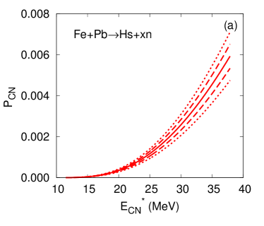
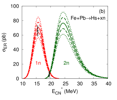
Figure 4: (a) The fusion probability for the reaction ${}_{26}^{58}\mbox{Fe}+_{\,\,\,82}^{208}\mbox{Pb}\rightarrow_{\,\,\,\,\,\,\,\,108}^{266-x}\mbox{Hs}+x\mbox{n}$. The solid line represents the phenomenological formula given by Eq. (60), the dashed lines include $10\%$ coupling effects compared to the phenomenological formula, and the dotted lines include $20\%$ coupling effects. (b) The cross section of the evaporation residue for the reaction ${}_{26}^{58}\mbox{Fe}+_{\,\,\,82}^{208}\mbox{Pb}\rightarrow_{\,\,\,\,\,\,\,\,108}^{266-x}\mbox{Hs}+x\mbox{n}$. The red lines are for the $1\mbox{n}$ channel, and the green lines are for the $2\mbox{n}$ channel. The solid lines are calculated with the fusion probability given by Eq. (60), the dashed lines include $10\%$ coupling effects on the fusion probability, and the dotted lines include $20\%$ coupling effects. The black points represent the experimental data with errorsAdamian et al. (2004).

Fig. 4(a) shows the fusion probability depending on the excitation energy. The solid line is calculated with the phenomenological formula in Eq. (60), the dashed lines include $10\%$ coupling effects compared to the phenomenological formula, and the dotted lines include $20\%$ coupling effects. We mention that $10\,$-$\,20\%$ effects are caused by corrections to both the quasifission rate and the fusion rate. The fusion probability generally grows as the excitation energy increases. The degree of increase depends on the degree of couplings. Fig. 4(b) shows the cross section of evaporation residue calculated by Eq. (57). The red lines are for the $1$n evaporation channel, and the green lines are for the $2$n channel. The solid lines are calculated with the fusion probability given by the phenomenological formula. The dashed and dotted lines are calculated with the fusion probability including $10\%$ and $20\%$ coupling effects, respectively. As the excitation energy increases, the cross section initially grows and then decreases due to the survival probability. At the maximum of the cross section, the coupling effect is largest. The black points show the experimental data with errorsAdamian et al. (2004). The cross section calculated with the phenomenological fusion probability agrees with the experimental data within the errors. However, the coupling effects might produce uncertainties on the cross section. We note that the magnitude of the error is comparable to $10\,$-$\,20\%$ coupling effects at the maximum of the cross section.

We should mention that there are other factors contributing to the uncertainties of the cross section, in addition to the coupling effects between two collective modes of a dinuclear system. Especially, the degree of the survival probability highly depends on calculation methods and parameter values. However, in Fig. 4 we present the degree of the coupling effects for a reaction in which the calculated cross section agrees with the experimental data.

V Summary and Discussions

In this work, we considered the Kramers’ escape problem with two collective modes and calculated the diffusion rates in the weak coupling limit. Due to the coupling through the inverse mass tensors, the rates have corrections depending on the friction coefficients and the angular frequencies at the barriers. Our results are given by Eqs.(31), (38), (42), and (45). They can be generally applied to any escape problem in a quantum mechanical system with friction and diffusion.

We have applied the escape problem to a dinuclear system to estimate the fusion probability. For the coefficients of $\hbar\omega_{R_{b}}=2\,\mbox{MeV}$, $\hbar\omega_{\eta_{b}}=1\,\mbox{MeV}$, and $\hbar\gamma_{R}^{*}=\hbar\gamma_{\eta}^{*}=2\,\mbox{MeV}$, we present the coupling effects on the diffusion rates in Fig. 2. The fusion rate changes up to $30\%$ while the quasifission rate is barely affected by comparison. Since the fusion probability is determined by the diffusion rates of two collective modes, the couplings affect the fusion probability and the cross section of evaporation residue. Fig. 4 shows $10\,$-$\,20\%$ coupling effects for the reaction ${}_{26}^{58}\mbox{Fe}+_{\,\,\,82}^{208}\mbox{Pb}\rightarrow_{\,\,\,\,\,\,\,\,108}^{266-x}\mbox{Hs}+x\mbox{n}$ ($x=1,2$). The effects depend on the excitation energy, and they are the largest at the maximum of the cross section. While the calculated cross section agrees with data, the experimental uncertainties are comparable to $10\,$-$\,20\%$ coupling effects at the maximum of the cross section.

We should mention that there are other uncertainties in estimating the cross section of evaporation residue. Some of the effects might be greater than the coupling effects on the fusion probability. Especially, the survival probability highly depends on the calculation methods and parameter values. However, the purpose of this work is to investigate the coupling effects on the fusion probability for more quantitative analysis of data. We calculated the leading order corrections to the quasifission rate and the fusion rate. The effects of each coupling might be important to understand fusion depending on reactions. Since we do not have complete understanding of fusion dynamics nor nuclear data in details, we need a phenomenological strategy to compare the analytical results with experiments.

We focused on asymmetric dinuclear systems in the presence of the coupling through the inverse mass tensors. We need many assumptions to obtain Eq. (2), but the general description of a dinuclear system involves other effects. First, we ignored $\partial\mu_{R}/\partial R$ and $\partial\mu_{\eta}/\partial\eta$ which might be important in some reactions. Second, we have non-diagonal components of the inverse mass tensor, the friction tensor, and the diffusion tensor as well as the diagonal components of the kinetic energy. By including those terms, the coupling between the relative motion and the mass asymmetry might be related to the neck dynamics. Third, we used a locally harmonic approximation, but the diabatic potential might need anharmonic corrections. Finally, the Fokker-Planck equation can be extended to include the second derivatives with respect to collective coordinates (and with respect to a collective coordinate and the corresponding conjugate momentum)Palchikov et al. (2002). In principle, all the above effects can be calculated in a similar way used in this work. We hope to discuss the general analysis in future presentations.

ACKNOWLEDGMENTS

We would like to thank G. G. Adamian and N. V. Antonenko for useful discussions and for providing their numerical code to calculate the diabatic potential. This work is supported by the Rare Isotope Science Project of Institute for Basic Science funded by Ministry of Science, ICT and Future Planning and National Research Foundation of Korea (2013M7A1A1075766).

References

- Zagrebaev et al. (2001) V. I. Zagrebaev, Y. Aritomo, M. G. Itkis, Y. T. Oganessian, and M. Ohta, Phys. Rev. C. 65, 014607 (2001).
- Adamian et al. (1997a) G. G. Adamian, N. V. Antonenko, and W. Scheid, Nucl. Phys. A 618, 176 (1997a).
- Swiatecki et al. (2005) W. J. Swiatecki, K. Siwek-Wilczynska, and J Wilczynski, Phys. Rev. C. 71, 014602 (2005).
- Liu and Bao (2006) Z. H. Liu and J. D. Bao, Phys. Rev. C. 74, 057602 (2006).
- Volkov (1978) V. V. Volkov, Phys. Rept. 44, 93 (1978).
- Hanggi et al. (1990) P. Hanggi, P. Talkner, and M. Borkovec, Rev. Mod. Phys. 62, 251 (1990).
- Adeev and Gonchar (1985) G. D. Adeev and I. I. Gonchar, Z. Phys. A 320, 451 (1985).
- Langer (1969) J. S. Langer, Ann. Phys. 54, 258 (1969).
- Weidenmuller and Jing-Shang (1984) H. A. Weidenmuller and Z. Jing-Shang, J. Stat. Phys. 34, 191 (1984).
- Kramers (1940) H. A. Kramers, Physica VII, no 4, 284 (1940).
- Pollak et al. (1990) E. Pollak, S. C. Tucker, and B. J. Berne, Phys. Rev. Lett. 65, 1399 (1990).
- Talkner (1995) P. Talkner, New Trends in Kramers’ Reaction Rate Theory, P. Talkner and P. Hanggi, eds., Dordrecht , 47 (1995).
- Adamian et al. (1995) G. G. Adamian, N. V. Antonenko, and R. V. Jolos, Nucl. Phys. A 584, 205 (1995).
- Adamian et al. (2014) G. G. Adamian, N. V. Antonenko, and A. S. Zubov, Phys. Part. Nucl. 45, 848 (2014).
- Antonenko et al. (1995) N. V. Antonenko, E. A. Cherepanov, A. K. Nasirov, V. P. Permjakov, and V. V. Volkov, Phys. Rev. C. 51, 2635 (1995).
- Adamian et al. (1997b) G. G. Adamian, N. V. Antonenko, W. Scheid, and V. V. Volkov, Nucl. Phys. A 627, 361 (1997b).
- Adamian et al. (1998) G. G. Adamian, N. V. Antonenko, W. Scheid, and V. V. Volkov, Nucl. Phys. A 633, 409 (1998).
- Wong (1973) C. Y. Wong, Phys. Rev. Lett. 31, 766 (1973).
- Migdal (1967) A. B. Migdal, “Theory of finite fermi systems and application to atomic nuclei,” (1967).
- Zubov et al. (2003) A. S. Zubov, G. G. Adamian, N. V. Antonenko, S. P. Ivanova, and W. Scheid, Phys. Rev. C. 68, 014616 (2003).
- Adamian et al. (2004) G. G. Adamian, N. V. Antonenko, A. Diaz-Torres, and W. Scheid, Acta. Phys. Hung. A 19/1-2, 87 (2004).
- Cherepanov et al. (1983) E. A. Cherepanov, A. S. Iljinov, and M. V. Mebel, J. Phys. G. 9, 931 (1983).
- Zubov et al. (2002) A. S. Zubov, G. G. Adamian, N. V. Antonenko, S. P. Ivanova, and W. Scheid, Phys. Rev. C. 65, 024308 (2002).
- Vandenbosch and Huizenga (1974) R. Vandenbosch and J. R. Huizenga, “Nuclear fission,” (1974).
- Schmidt and Morawek (1991) K. H. Schmidt and W. Morawek, Rep. Prog. Phys. 54, 949 (1991).
- Moller et al. (1995) P. Moller, J. R. Nix, W. D. Myers, and W. J. Swiatecki, At. Data. Nucl. Data. Tables. 59, 185 (1995).
- Moller et al. (1997) P. Moller, J. R. Nix, and K. L. Kratz, At. Data. Nucl. Data. Tables. 66, 131 (1997).
- Palchikov et al. (2002) Y. V. Palchikov, G. G. Adamian, N. V. Antonenko, and W. Scheid, Physica A 316, 297 (2002).