Complete Photoionization Experiments via Ultrafast Coherent Control with Polarization Multiplexing II:
Numerics & Analysis Methodologies

Abstract

The feasibility of complete photoionization experiments, in which the full set of photoionization matrix elements are determined, using multiphoton ionization schemes with polarization-shaped pulses has recently been demonstrated [Hockett et. al., Phys. Rev. Lett. 112, 223001 (2014)]. Here we extend on our previous work to discuss further details of the numerics and analysis methodology utilised, and compare the results directly to new tomographic photoelectron measurements, which provide a more sensitive test of the validity of the results. In so doing we discuss in detail the physics of the photoionziation process, and suggest various avenues and prospects for this coherent multiplexing methodology.

I Introduction

The aim of “complete” photoionization studies is the determination of the amplitudes and phases of the ionization matrix elements, which constitute a fundamental description of an ionization event Reid2003 ; Cherepkov2005 . The matrix elements define the coupling of the initial state to the final compound state, comprised of an ion and free electron. In the dipole limit, this matrix element can be very generally defined as $\langle\psi^{e};\,\Psi^{+}|\hat{\boldsymbol{\mu}}.\mathbf{E}|\Psi\rangle$. Here $\Psi$ is the initial wavefunction of the system, $\Psi^{+}$ the photoion, $\psi^{e}$ the photoelectron, $\hat{\boldsymbol{\mu}}$ the dipole operator and $\mathbf{E}$ the electric field. By expressing the continuum wavefunction $\psi^{e}$ as a set of partial-waves, corresponding to different continuum angular momentum states, the ionization matrix element can be decomposed into various geometric and radial components, and the set of amplitudes and phases of these components constitutes a complete description of the ionization event. In order to determine these matrix elements from experimental data, an observable sensitive to the relative phases of the partial-waves is required, and such an interferometric observable is found in the photoelectron angular distributions (PADs), which are angular interference patterns dependent on the composition of $\psi^{e}$.

A range of experiments have been performed in order to provide such complete descriptions of photoionization for a number of atomic and molecular systems. The key concern in such experiments is the level of detail required in order to undertake the relatively complex analysis procedure. Typically the angular (or geometric) part of the matrix elements can be calculated analytically Dill1976 , leaving only the energy-dependent radial (or dynamical) components to be determined from the experimental data. The determination of these components involves fitting experimental data with the specific ionization formalism for the ionization event under study. Since, in general, there may be many partial-waves and the composition of $\psi^{e}$ is not usually known a priori, a large experimental dataset is required for this procedure. In order to obtain a sufficient dataset, experimental data is obtained for a range of geometric parameters, for example by varying the polarization state and polarization geometry Lambropoulos1973 ; berry1976 ; Duong1978 ; Hansen1980 ; Chien1983 or, for molecules, the rotational state or axis distribution Reid1991 ; Reid1992 ; Suzuki2006 ; Hockett2009 ; Suzuki2012 , or via molecular frame measurements Gessner2002 ; Lebech2003 ; Yagishita2005 . Since the dynamical parameters are invariant to these geometric changes, a dataset of sufficient information content to determine these parameters may be obtained in this way.

Recently, we demonstrated a new type of measurement and analysis methodology for complete experiments Hockett2014 . This method can be considered as time-domain polarization-multiplexing. In this case, a multiphoton ionization scheme with a moderately intense, ultrafast laser pulse was employed to ionize potassium atoms. The resulting light-matter interaction can be understood as an intra-pulse two-step processes, in which electronic population transfer is driven by the laser field (i.e. Rabi oscillations), and the excited state population created can subsequently be ionized via 2-photon absorption. In this case, the population dynamics and the ionization dynamics are dependent on the properties of the laser pulse, as well as the physical properties of the system which ultimately determine the matrix elements. In this scheme, changing the polarization of the pulse corresponds to changing the geometric parameters of the ionization, as described above. In the simplest case a single or pure polarization state is employed, and the geometric parameters are time-invariant. More generally, via the use of a polarization-shaped pulse, the geometric parameters can be changed in a time-dependent manner. Since the dynamics and ionization all occur within a single laser pulse, the process is fully-coherent, and the final, time-integrated, photoelectron measurement can be considered as a time-domain multiplexed measurement of the set of (instantaneous) polarization states explored by the shaped-pulse.

Here we discuss further details of the work presented in ref. Hockett2014 , with a focus on extending the details of the theory presented therein, in particular the numerical details of the fitting procedure and a discussion of the benefits and limitations of this approach. We further present detailed comparison of our results with new maximum information photoelectron measurements, utilizing a tomographic procedure for the measurement of 3D photoelectron distributions and detailed analysis, allowing for a quantitative comparison of the predicted PADs and experimental PADs as a function of polarization geometry (further details of the maximum information measurements can be found in ref. Hockett2015b ). Finally, the possibilities of extending this treatment to different classes of ionization is explored, with a particular emphasis on molecular ionization problems.

II Intrapulse dynamics & multiphoton ionization with polarization-shaped pulses

Here we detail the various steps involved in the treatment of the 3-photon scheme detailed above. For completeness we include all aspects of our treatment.

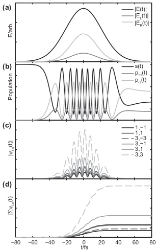
Figure 1: Time-dependent dynamics for an elliptically polarized laser pulse. (a) Laser field envelope for an elliptically polarized pulse, defined by $\phi_{y}=0.5$ rad (eqn. 5). (b) Bound state populations (eqn. 6). (c) Instantaneous continuum populations $d_{l_{f},m_{f}}(k,t)$ (eqn. 17) and (d) cumulative continuum population (eqn. 18).

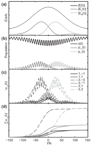
Figure 2: Time-dependent dynamics for a polarization-shaped laser pulse. (a) Laser field envelope for an elliptically polarized pulse, defined by $\phi_{y}=-\pi$ rad for the blue half of the pulse (eqn. 5). (b) Bound state populations (eqn. 6). (c) Instantaneous continuum populations $d_{l_{f},m_{f}}(k,t)$ (eqn. 17) and (d) cumulative continuum population (eqn. 18).

II.1 Electric field

The electric field as a function of time is described as:

$$E(t)=E_{0}e^{-(t/\tau)^{2}}e^{i\omega t}$$ (1)

where $E_{0}$ is the field strength, the pulse envelope is Gaussian with temporal width parameter $\tau$ and $\omega$ is the carrier (angular) frequency. Using the notation of ref. dielsandrudolph the spectral content of the pulse is given by:

$$\tilde{E}(\Omega)=\mathcal{F}\{E(t)\}$$ (2)

where $\mathcal{F}$ represents a Fourier Transform.

Polarization shaped pulses are described as in ref. Wollenhaupt2009a , by assuming initially identical and in-phase $(x,y)$ field components, then applying a spectral phase shift. Hence, a field described by two Cartesian components with independent spectral phases (but identical spectral content) can be defined as:

$$\left(\begin{array}[]{c}\tilde{E_{x}}(\Omega)\\ \tilde{E_{y}}(\Omega)\end{array}\right)=\tilde{E}(\Omega)\left(\begin{array}[]{c}e^{i\phi_{x}(\Omega)}\\ e^{i\phi_{y}(\Omega)}\end{array}\right)$$ (3)

resulting in the time-domain components:

$$\left(\begin{array}[]{c}E_{x}(t)\\ E_{y}(t)\end{array}\right)=\mathcal{F}^{-1}\left\{\tilde{E}(\Omega)\left(\begin{array}[]{c}e^{i\phi_{x}(\Omega)}\\ e^{i\phi_{y}(\Omega)}\end{array}\right)\right\}$$ (4)

The field can also be expressed in terms of a spherical basis, i.e. left and right circularly polarized components:

$$\left(\begin{array}[]{c}E_{L}(t)\\ E_{R}(t)\end{array}\right)=\frac{1}{\sqrt{2}}\left(\begin{array}[]{c}E_{x}(t)-iE_{y}(t)\\ E_{x}(t)+iE_{y}(t)\end{array}\right)$$ (5)

This final form was used in the calculations herein, since it physically describes the instantaneous pulse angular momentum, in terms of the projection of the photon momentum onto the propagation axis, where $L$ equates to $m=+1$ and $R$ to $m=-1$ states. This form can therefore be directly interpreted in terms of the allowed $\Delta m$ of both bound-bound and bound-free transitions - this is discussed further below. Note that this form implies that the light propagates along the $z$-axis, and the lab. frame angular momentum $m$ is defined relative to this propagation axis.

II.2 Non-perturbative laser-atom interaction

The strong laser field drives Rabi oscillations in the atom, coupling electronic states $|n,l,m\rangle$. In the case of potassium atoms, as detailed in ref. Wollenhaupt2009a , the initial population is in the 4$s$ state and the laser frequency is near resonant with the $|4,0,0\rangle\rightarrow|4,1,m\rangle$ transition, hence single photon absorption populates the 4$p$ manifold, while a strong laser field will drive Rabi cycling between the $4s$ and $4p$ states. The allowed values of $m$ depend on the polarization state of the light.

The population dynamics during the laser pulse, described in the spherical basis of eqn. 5, are given by the time-dependent Schrödinger equation:

$$\frac{d}{dt}\left(\begin{array}[]{c}s(t)\\ p_{+1}(t)\\ p_{-1}(t)\end{array}\right)=i\left(\begin{array}[]{ccc}0&\frac{1}{2}\Omega_{L}^{*}(t)&\frac{1}{2}\Omega_{R}^{*}(t)\\ \frac{1}{2}\Omega_{L}(t)&\delta_{+1}&0\\ \frac{1}{2}\Omega_{R}(t)&0&\delta_{-1}\end{array}\right)\left(\begin{array}[]{c}s(t)\\ p_{+1}(t)\\ p_{-1}(t)\end{array}\right)$$ (6)

where $s(t)$, $p_{+1}(t)$ and $p_{-1}(t)$ are the state vector components for the $|4,0,0\rangle$ and $|4,1,\pm 1\rangle$ states, $\Omega_{L/R}(t)=\mu_{L/R}E_{L/R}(t)$ where $\mu_{L/R}$ are the transition amplitudes, and $\delta_{\pm 1}$ represent the detuning of the laser from the resonant frequency of the transition. Here it is clear that the $L$ and $R$ components of the electric field drive transitions with $\Delta m=+1$ and $\Delta m=-1$ respectively; this is simply the consequence of the conservation of angular momentum since the light carries $l=1$ unit of angular momentum, with lab. frame projection $m=1$ for $E_{L}$ and $m=-1$ for $E_{R}$. In this sense the (instantaneous) helicity of the electric field is directly imprinted on the atomic ensemble.

Here $\hbar$ and $E_{0}$ are both set to unity for simplicity; $\mu_{L/R}$ is also set to unity, i.e. equal probability of transitions to both $|4,1,m\rangle$ states, and $\delta_{\pm 1}=0.05$ rad/fs. For determination of PADs these simplifications are acceptable as only the relative population of $m=\pm 1$ states will affect the angular distribution, and these populations are dependent only on the driving laser field polarization.

II.3 Perturbative two-photon ionization & PADs

In the perturbative regime, the dipole transition amplitude for a transition from a bound state $|n_{i},l_{i},m_{i}\rangle$ to a continuum state $|\mathbf{k};\,l_{f},m_{f}\rangle$ is given by the dipole matrix elements:

$$d_{i\rightarrow f}(k,t) = \langle\mathbf{k};\,l_{f}m_{f}|\hat{\boldsymbol{\mu}}_{if}.E(t)|n_{i}l_{i}m_{i}\rangle$$ (7)

$$\propto R_{l_{i}l_{f}}^{n}(k)E_{q}(t)\langle l_{f}m_{f},1q|l_{i}m_{i}\rangle$$ (8)

where $\boldsymbol{\hat{\mu}}_{if}$ is the dipole operator; $R_{l_{i}l_{f}}^{n}(k)$ is the radial part of the matrix element, which is dependent on the magnitude of the photoelectron wavevector $\mathbf{k}$, the principal quantum number of the initial state $n$ and the electronic orbital angular momentum $l$, but assumed to be independent of $m_{i}$ and $m_{f}$; $\langle l_{f}m_{f},1q|l_{i}m_{i}\rangle$ is a Clebsch-Gordan coefficient which describes the angular momentum coupling for single photon absorption, with $q=\pm 1$ for the $L$ and $R$ components of the laser field respectively. This treatment corresponds to a single active electron picture, in which the final state is a pure continuum state, i.e. the photoion is neglected and there is no angular momentum transfer to core. Spin is also neglected. This treatment is sufficient for the potassium atom case discussed herein; extension to more complex coupling schemes is discussed in sect. V.

Under these assumptions, the angular part of both bound-bound and bound-free transitions are described by matrix elements of the same form. Using these dipole matrix elements, two-photon ionization to a single final state $|l_{f},m_{f}\rangle$, from an initial state $|n_{i},l_{i},m_{i}\rangle$, via a virtual one-photon state $|n_{v},l_{v},m_{v}\rangle$, can then be written as:

$$d_{l_{f}m_{f}}(k,t) = d_{i\rightarrow v}(k,t)d_{v\rightarrow f}(k,t)$$ (9)

$$= \sum_{\begin{array}[]{c}n_{i},l_{i},m_{i}\\ n_{v},l_{v},m_{v}\\ q,q^{\prime}\end{array}}R_{l_{v}l_{f}}^{n_{v}}(k)E_{q^{\prime}}(t)\langle l_{f}m_{f},1q^{\prime}|l_{v}m_{v}\rangle R_{l_{i}l_{v}}^{n_{i}}(k)E_{q}(t)\langle l_{v}m_{v},1q|l_{i}m_{i}\rangle\chi_{n_{i},l_{i},m_{i}}(t)$$ (13)

This form shows the general case, with summation over all initial states $|n_{i},l_{i},m_{i}\rangle$ weighted by their populations $\chi_{n_{i},l_{i},m_{i}}(t)$. Although the bound-free matrix element is labelled with quantum number $n_{v}$, in practice this is unassigned and will correspond to a quasi-continuum of virtual states within the laser bandwidth, so is dropped in the following. In this treatment all energy dependence is contained in the $R(k)$ radial integrals. For the potassium case considered here, a slightly simplified form can be written since only the 4$p$ levels contribute to the ionization, hence $n_{i}=4$, and the time-dependent populations are given by $p_{m_{i}}(t)$ as defined in eqn. 6:

$$d_{l_{f}m_{f}}(k,t) = \sum_{\begin{array}[]{c}l_{i},m_{i}\\ l_{v},m_{v}\\ q,q^{\prime}\end{array}}R_{l_{v}l_{f}}(k)E_{q^{\prime}}(t)\langle l_{f}m_{f},1q^{\prime}|l_{v}m_{v}\rangle R_{l_{i}l_{v}}^{(4)}(k)E_{q}(t)\langle l_{v}m_{v},1q|l_{i}m_{i}\rangle p_{m_{i}}(t)$$ (17)

Integrating over $t$ yields:

$$d_{l_{f}m_{f}}(k)=\int d_{i\rightarrow v}(k,t)d_{v\rightarrow f}(k,t)dt=\int dt\sum_{\begin{array}[]{c}l_{i},m_{i};l_{v},m_{v}\\ q,q^{\prime}\end{array}}R_{l_{v}l_{f}}(k)\langle l_{f}m_{f},1q^{\prime}|l_{v}m_{v}\rangle R_{l_{i}l_{v}}^{(4)}(k)\langle l_{v}m_{v},1q|l_{i}m_{i}\rangle E_{q^{\prime}}(t)E_{q}(t)p_{m_{i}}(t)$$ (18)

The observed photoelectron yield as a function of angle, the PAD, for a small energy range $dk$ over which we assume the $R(k)$ are constant, is then given by the coherent square over all final (photoelectron) states:

$$I(\theta,\phi;\,k) =\int dk \sum_{\begin{array}[]{c}l_{f},m_{f}\\ l_{f}^{{}^{\prime}},m_{f}^{{}^{\prime}}\end{array}}d_{l_{f}m_{f}}(k)Y_{l_{f}m_{f}}(\theta,\phi)d_{l_{f}^{{}^{\prime}}m_{f}^{{}^{\prime}}}^{*}(k)Y_{l_{f}^{{}^{\prime}}m_{f}^{{}^{\prime}}}^{*}(\theta,\phi)$$ (21)

This treatment is very similar to that given in ref. Wollenhaupt2009a , with the Clebsch-Gordan coefficients equivalent to the $\alpha_{l,m;l^{\prime},m^{\prime}}$ parameters and the $d_{l_{f}m_{f}}$ similar to the $c_{l,m}$. The main difference is that all $|l_{f},m_{f}\rangle$ are accounted for, hence the explicit inclusion of the radial elements $R_{ll}(k)$. The radial matrix elements defined here are assumed to be complex, and include both the scattering phase $e^{-i\eta_{l}}$ and the geometric phase factor $i^{l}$ which usually appear in the definition of the photoelectron wavefunction Park1996 . The amplitudes and phases of these parameters constitute the unknowns which are sought in “complete” photoionization studies and, physically, define the scattering of the outgoing photoelectron from the nascent ion core.

The PAD can also be described by a generic expansion in spherical harmonics with expansion coefficients $\beta_{L,M}$, termed anisotropy parameters, where:

$$I(\theta,\phi;\,k)=\sum_{L,M}\beta_{L,M}(k)Y_{L,M}(\theta,\,\phi)$$ (22)

In general the $\beta_{L,M}(k)$ provide a compact way to express the PADs, and allowed values are constrained by symmetry Yang1948 ; Reid2003 . This expansion can be considered as indicating the information content of a given distribution, and the resultant multipole moments $L,\,M$ are related to the partial wave expansion of eqn. 22 by Reid1991 :

$$\beta_{L,M}=\underset{\begin{array}[]{c}l_{f},m_{f}\\ l_{f}^{{}^{\prime}},m_{f}^{{}^{\prime}}\end{array}}{\sum}\sqrt{\frac{(2l_{f}+1)(2l^{\prime}_{f}+1)(2L+1)}{4\pi}}\left(\begin{array}[]{ccc}l_{f}&l^{\prime}_{f}&L\\ 0&0&0\end{array}\right)\left(\begin{array}[]{ccc}l_{f}&l^{\prime}_{f}&L\\ m_{f}&-m^{\prime}_{f}&M\end{array}\right)d_{l_{f}m_{f}}(k)d_{l_{f}^{{}^{\prime}}m_{f}^{{}^{\prime}}}^{*}(k)$$ (23)

Further exploration of the information content of PADs for the case of tomographic 3D photoelectron measurements can be found in ref. Hockett2015b .

II.4 Pure and shaped laser pulse dynamics

In order to illustrate the theory detailed above, figures 1 and 2 give the details of two example calculations, for an elliptically polarized pulse and a fully polarization-shaped pulse respectively. In both cases the panels illustrate, from top to bottom, the envelope of the laser field and $L$, $R$ components, as defined by eqn. 5; the population dynamics driven by the laser field, in terms of the state vector components $s(t)$, $p_{+1}(t)$ and $p_{-1}(t)$ defined in eqn. 6; the instantaneous continuum populations, as defined by eqn. 17 and making use of the previously determined photoionization matrix elements $R_{ll}$ (see ref. Hockett2014 and sect. III); the cumulative continuum populations, as defined by eqn. 17.

Both examples provide insight into the dynamics of the ionization process, and it is clear how the $L$ and $R$ components of the laser field drive both the bound-state population dynamics, and the instantaneous continuum contributions. Since, in this model, the two steps are decoupled, and the ionization is assumed to be perturbative, there is no depletion in the bound state populations. The ionization step does, however, follow the bound state dynamics since the instantaneous population defines which continuum states can be accessed, and their relative weighting. Thus, the instantaneous continuum dynamics follow the bound-state dynamics. Furthermore, since there are no continuum electron dynamics in this model (i.e. no laser-continuum coupling, or electron-ion recombination), the final continuum is simply the sum over the instantaneous continuum contributions (eqn. 18) and builds up coherently over the pulse envelope. The resultant PAD, eqn. 21, thus depends both on the final continuum populations, as well as the accumulated phase for each $|l_{f},m_{f}\rangle$ state.

In the case of a “pure” polarization state (fig. 1), in this example an elliptically polarized light field defined by $\phi_{y}=0.5$ rad., there is essentially no dynamic contribution to the final result since the relative continuum contribution is time-independent. In the language used previously, the geometric contribution to the ionization is time-invariant. However, in the case of a polarization-shaped pulse (fig. 2), where the relative $L$ and $R$ components do vary significantly over the pulse, the intra-pulse dynamics play a key role in defining the final continuum wavefunction. It is this dependence that makes the final PAD particularly sensitive to the pulse shape, as well as the ionization matrix elements. While the two cases are formally identical, there is clearly no polarization multiplexing in the pure case, since the polarization state is time-invariant. In the polarization-shaped case, the information content is greatly increased since the final result arises from coherent addition over all instantaneous polarization states, thus contains additional information relative to a pure case. (Further examples of polarization-shaped pulses and resultant PADs can be found in ref. Hockett2014 .)

III Photoelectron image generation & fitting

In this section we outline salient details of the numerics used in applying the above theory to the generation of photoelectron momentum distributions which can be compared with experimental data. In the context of complete photoionization experiments, the use of these momentum distributions to generate 2D photoelectron images and fit experimental data is described.

III.1 Photoelectron momentum distributions

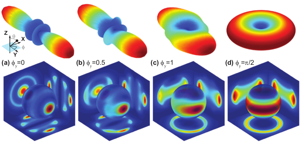
Figure 3: Illustration of computed PADs and 2D photoelectron images as a function of pulse polarization defined by $\phi_{y}$, propagating in the $z$-direction. The top row shows PADs in polar form, $I(\theta,\,\phi;\,k)$, the bottom row shows the same distributions projected onto a velocity iso-sphere (single $k$), and 2D image plane projections $I_{2D}(\theta_{2D},\,k)$ assuming a Gaussian energy spectrum.

The theory detailed above provides a definition of the photoelectron yield as a function of time, energy and angle, most compactly defined by the $\beta_{L,M}(k)$ parameters, but ultimately depending on the underlying laser and target properties. The generation of theoretical, time-integrated, photoelectron momentum distributions from these parameters simply involves the population of a 3D grid $(\theta,\phi,k)$ with the relevant basis set expansion in spherical harmonics as a function of energy, as defined in eqn. 21 (the radial aspect of this expansion is discussed below).

The volumetric data defined in this way is equivalent to the experimental data recorded in a 3D imaging experiment, examples of such experiments are direct 3D imaging via techniques with high temporal and spatial resolution (for instance refs. Continetti2001 ; Reid2012 ; Hockett2013 and references therein), or indirect methods based on tomography in which 3D distributions are reconstructed from a set of 2D projections Wollenhaupt2009 ; Smeenk2009 ; Hockett2010 (see also ref. Hockett2015b ). For comparison with 2D imaging data, further integration along a spatial dimension is additionally required in order to project the volumetric data onto a 2D plane. We note that in both imaging experiments and the numerics applied here, this summation is treated incoherently. Physically, this corresponds to a loss of photoelectron coherence before or at the detector, effectively long after the coherent quantum mechanical scattering event which determines the momentum distribution (PADs and energy spectrum) Wollenhaupt2002 ; Wollenhaupt2013 . Since the range of the initial scattering event is microscopic, while photoelectron propagation and detection is macroscopic and often involves the application of external fields and, ultimately, discrete particle counting, this is a physically reasonable assumption.

In the results shown in paper I we additionally assumed that the radial dependence of the ionization matrix elements over the span of the main spectral feature (~200 meV) was negligible, and that the details of the radial distribution could be simplified to a Gaussian energy spread with no phase contribution. This allowed for the momentum data generation and fitting to be simplified, and the radial distribution given by a Gaussian (defined in energy-space):

$$G(k)=\frac{I_{0}}{\sqrt{2\pi\gamma}}e^{-(E(k)-E(k_{0}))^{2}/2\gamma^{2}}$$ (24)

where $I_{0}$ is the intensity, $\gamma$ the width, $E(k)$ and $E(k_{0})$ define the radial coordinate and the peak centre in energy-space. The final 3D momentum distribution is then defined by:

$$I(\theta,\phi,k)=G(k)\sum_{L,M}\beta_{L,M}^{k}Y_{L,M}(\theta,\phi)$$ (25)

Where the $\beta_{L,M}^{k}$ include the superscript to denote that these parameters are generally dependent on $k$, as in eqn. 22, but are here taken to be constant over the range of $k$ spanned by the Gaussian envelope $G(k)$. Finally, it is of note that more generally the Gaussian assumed here should be replaced by an accurate energy spectrum, this point is discussed in sect. V.

The 2D images obtained by integration of the volumetric distribution function are then given as:

$$I_{2D}(\theta_{2D},k)=\intop_{u}I(\theta,\phi,k)\mathrm{d}u$$ (26)

where $u$ defines the domain of integration (with integration over the Cartesian $X$, $Y$ or $Z$ directions for the corresponding $(y,z)$, $(x,z)$ or $(x,y)$ image planes respectively), and $\theta_{2D}$ is defined in the image plane.

Figure 3 illustrates the computed PADs, obtained using the matrix elements of ref. Hockett2014 , for four polarization states of the electric field. The top row shows the PADs in spherical polar form, as defined by eqn. 22, while the bottom row shows the same PADs projected onto spherical surfaces. This is how the distributions appear in velocity space, as the angle-dependent photoelectron flux for each $k$. The 2D projections show the same angular distributions, combined with a Gaussian energy spectrum as per eqn. 25, and projected onto 2D Cartesian planes. These image planes simulate velocity map imaging data, and illustrate how the experimental results will depend on both the native details of the PAD and the details of the projection geometry. In this case, the laser propagates along the $Z$-axis, and the polarization is defined in the $(X,Y)$ plane, so experimental images will correspond to the image planes $(x,z)$ or $(y,z)$ (since images cannot be obtained in the propagation direction in a standard VMI experiment), and the precise details will further depend on the rotation of the distribution about the $Z$-axis. (Further details of 2D and 3D imaging, geometry considerations and information content, can be found in ref. Hockett2015b .)

III.2 Fitting methodology

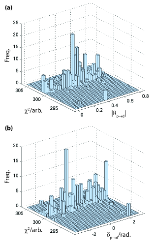
Figure 4: Example of fit statistics for $R_{p\rightarrow d}$, (a) magnitude, (b) phase.

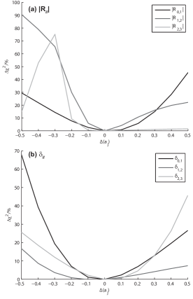
Figure 5: 1D cuts through the $\chi^{2}$ hypersurface for (a) magnitudes and (b) phases of the $R_{i\rightarrow f}$ matrix elements. Cuts are made by varying each parameter by $\Delta a_{j}$, here given as a fractional variation from the best fit value (i.e. test value $a^{\prime}_{j}=a_{j}+(a_{j}\times\Delta a_{j})$, and $a^{\prime}_{j}=a_{j}$ for $\Delta a_{j}=0$), and the resulting change in $\chi^{2}$ is given as a percentage relative to the best fit value.

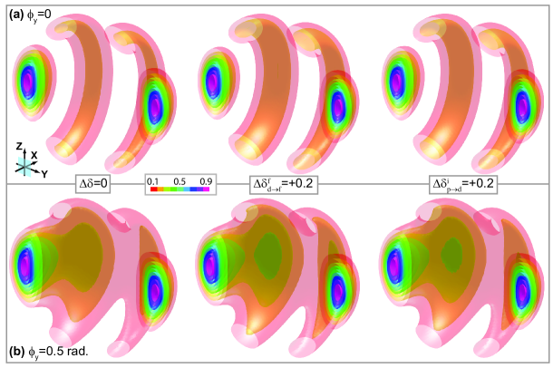
Figure 6: Calculated 3D distributions $I(\theta,\phi,k)$ (first column) and sensitivity to changes in the phases $\delta_{d\rightarrow f}^{f}$ and $\delta_{p\rightarrow d}^{i}$ for (a) linear polarization and (b) elliptical polarization $\phi_{y}=0.5$ rad.

As discussed above, within the framework developed herein the radial matrix elements are the only unknown quantities. With a sufficient experimental dataset one can therefore hope to obtain these matrix elements via a fit to the data. In this case the results of such a fit have already been presented in ref. Hockett2014 , and validated via good agreement with both the original 2D imaging data, and additional 3D data obtained via tomographic imaging experiments. We discuss here further details of the fitting methodology applied, since in general it is necessary to approach this complicated problem carefully. In particular, we applied statistical analysis methodologies which were previously developed for energy-domain photoionization experiments Hockett2009 ; hockettThesis .

In our procedure, the data from 2D measurements was compared with the calculated 2D images, as illustrated in figure 3 and obtained as detailed above. The calculated images were then optimized via a fitting routine, with the radial matrix elements and image generation parameters as the free parameters for fitting. The criteria for the best fit was simply the minimization of the sum of least squares:

$$\chi^{2}=\sum_{\theta_{2D},k}(I_{2D}(\theta_{2D},k)-I_{Expt.}(\theta_{2D},k))^{2}$$ (27)

where $I_{2D}$ is the calculated distribution defined in eqn. 26, and $I_{Expt.}$ the 2D experimental data. This methodology is completely general, and only relies on the underlying theoretical framework correctly describing the physics inherent to the problem. However, the size of the $\chi^{2}$ hyperspace may be very large since it has dimensions equal to the number of free fitting parameters. The practical outcome of this is that the possibility of local minima in the hyperspace is significant, and the parameters obtained via such a procedure must be carefully evaluated and tested to confirm their veracity and robustness.

In this particular case, the full calculation required 12 parameters, consisting of the amplitudes and phases of the 5 radial matrix elements $R_{ll}$ and 2 image generation parameters (Gaussian centre and FWHM) . Since absolute phases cannot be determined, one phase is chosen to be a reference and set to zero, leaving 11 free fit parameters. Furthermore, the image generation parameters do not have a large influence on the final results, which are primarily sensitive to the angular coordinate, and could therefore be bounded quite tightly after some initial by eye optimization, thereby reducing the search-space of physical relevance to, effectively, 9 dimensions. In the fitting procedure the $R_{ll}$ were expressed in magnitude and phase form, $R_{ll}=|R_{ll}|e^{i\delta_{ll}}$, where $0\leq R_{ll}\leq 1$, $-\pi\leq\delta_{ll}\leq\pi$, and $R_{l_{1}\rightarrow l_{2}}=R_{l_{2}\rightarrow l_{1}}^{*}$. Fitting was implemented with a standard fitting algorithm, Matlab’s lsqcurvefit, based on a Trust-Region-Reflective least-squares method. The dataset for fitting consisted of four experimental images, each corresponding to a different pure polarization state of the light, similar to the states shown in figure 6. The laser pulse was modelled with $\tau=30$ fs and four polarization states given by $\phi_{y}=0$ (linear polarization, ellipticity $\varepsilon=0$), $\phi_{y}=\pi/8,\,\pi/4$ (elliptical polarization states, with ellipticities $\varepsilon\sim$0.2, 0.4) and $\phi_{y}=\pi/2$ (circular polarization, $\varepsilon=1$). The ellipticities given here are defined as the ratio of the minor to major axes of the polarization ellipse, hence $\varepsilon=0$ for linearly polarized light and $\varepsilon=1$ for pure circularly polarized light. Because the elliptical polarization states may be slightly different from those obtained experimentally (via the use of a quarter-wave plate, see ref. Hockett2014 and refs. therein for further experimental details) the subsequent fitting was weighted towards the linear and circular polarization results by an additional factor of two in $\chi^{2}$.

In order to carefully test for local minima the hyperspace was repeatedly sampled using a Monte-Carlo approach, in which the fitting was repeated $N$-times with the seed values for the fitting parameters randomized on each iteration. Statistical analysis of the fitted parameters derived from such repeated fits can be employed to probe the behaviour of the fitting algorithm, and also to gain information on how well the experimental data defines each fitted parameter. Although it is non-trivial to visualize the full $\chi^{2}$ hypersurface, aspects can be probed by plotting histograms and correlation plots of the fitted parameters. A large scatter in the value of a given fit parameter over a range of fits to the same data suggests a poorly defined parameter; a consistent result meanwhile shows that a particular parameter is well defined by the dataset. The experimental data can show different sensitivities to different parameters depending on the type of ionizing transitions present, because different transitions will (according to the magnitude of the geometrical parameters and symmetry constraints) be more sensitive to certain partial-waves. Additionally, the presence of multiple-minima in the fit may be revealed by the presence of more than one feature in the histogram, reflecting more than one “best” fit result, while correlations appearing between supposedly uncorrelated parameters can indicate emergent behaviours in the high-dimensional space or - more prosaically - issues with the fitting methodology or coding.

In this case we performed 300 fits, and the lowest $\chi^{2}$ was obtained on 4 of these fits, which we take to be the absolute minimum. The radial matrix elements ultimately found, as reported in ref. Hockett2014 , are given in table 1 for reference, and discussed further below. Figure 4 gives an illustrative example of the fitting statistics, in this case showing correlation histograms between $\chi^{2}$ and the (a) magnitude and (b) phase of $R_{p\rightarrow d}$. The plot shows the 40 fit results within 5% of the lowest $\chi^{2}$. Interestingly, in this case many of the fits are bunched, with $\chi^{2}\sim 300$ (arb. units). This most likely reflects the presence of local minima as defined above, but may also be related to the convergence criteria set on the fitting algorithm which, in this case, was set to a limited number of iterations in order to cap the computational time per fit and ensure a large seed-space for the search; in effect the large seed-space becomes part of the fitting criteria. Depending on the seed values, the overall convergence of the fit may be fast or slow, and the possibility of finding the global minima will vary depending on the start position in the 11-dimensional parameter-space, as well as the topography of this space and the details of the fitting algorithm. From the histograms of the bunched results, it is apparent that $|R_{p\rightarrow d}|$ is somewhat well-defined at the larger $\chi^{2}$, with values mostly close to the best result, while the phase appears much less well-defined at this level. At lower $\chi^{2}$, the parameter-space is much sparser, with only a few parameter sets found, but they appear to converge on a single parameter set. These observations illustrate the difficulty in assessing best fit results without careful analysis: in this case sampling of only a few fit results would potentially lead to a parameter set quite different from the global optimal found. Here statistical analysis, as well as further validation of the results against additional experimental data (see sect. IV), both serve to provide confidence that the absolute best fit, hence physically correct, results have been obtained.

Transition			$|R_{l_{1}l_{2}}|$	$|R_{l_{1}l_{2}}|^{2}$/%	$\delta_{l_{1}l_{2}}$/rad.
	$l_{1}$	$l_{2}$
$i\rightarrow v$	p	s	0.34 (3)	12 (4)	0 *
	p	d	0.94 (8)	88 (11)	-1.62 (4)
$v\rightarrow f$	s	p	0.85 (8)	72 (12)	-0.19 (3)
	d	p	0.14 (2)	2 (2)	-2.08 (8)
	d	f	0.51 (9)	26 (13)	0.24 (7)

Table 1: Fitted values for the relative transition matrix element magnitudes, $|R_{ll}|$, and phases, $\delta_{ll}$. The square of the magnitudes is expressed as a percentage of the total transition amplitude, normalized to unity for each step. Uncertainties in the last digit are given in parentheses. * reference phase, set to zero during fitting.

III.3 Robustness, uncertainties & validation

As well as statistically evaluating fit results, the behaviour of $\chi^{2}$ can also be more directly probed. In essence, this amounts to removing the black-box nature of the fitting algorithm by explicitly looking at the gradient and curvature of $\chi^{2}$ as a function of the fitting parameters, rather than looking at only the final fitted results. Additionally, the curvature with respect to a given parameter can be used to provide uncertainty estimates on the fitted parameters bevington :

$$\sigma_{j}^{2}=2\left(\frac{\partial^{2}\chi^{2}}{\partial a_{j}^{2}}\right)^{-1}$$ (28)

where $\sigma_{j}$ is the uncertainty in parameter $a_{j}$. Equation 28 relates the response of $\chi^{2}$ to a given parameter; the sharper the response the better $a_{j}$ is defined by the data and hence the smaller the uncertainty. In practice this procedure equates to varying each fitted parameter by $\Delta a_{j}$, and evaluating $\chi^{2}$ for this new parameter set, in order to map out 1D cuts through the $\chi^{2}$ hypersurface. Uncertainties estimated in this manner were given in ref. Hockett2014 , and are provided again in table 1. It is also of note that a similar, but not identical, procedure can be performed by refitting all other $(n-1)$ parameters as a function of a test parameter $a_{j}$ Gessner2002 . This procedure will also provide 1D cuts through the hypersurface, but along the $n$-dimensional topography of the minimum. The drawback of this alternative procedure is the necessity of performing many additional fits, which may be computationally expensive; for this reason it was not explored in this work.

Figure 5 shows 1D cuts through the $\chi^{2}$ hyperspace as defined above, for the magnitudes and phases of $R_{i\rightarrow f}$. In this case it is clear that the sensitivity of $\chi^{2}$ is good in most cases, with 10 % changes in $a_{j}$ (i.e. $\Delta a_{j}=\pm 0.1$) typically leading to clear changes in $\chi^{2}$; this is also reflected in the relatively small uncertainties $\sigma_{j}^{2}$ given in table 1. In this case, a notable exception is $|R_{2\rightarrow 3}|$, which is much less sensitive to $\Delta a_{j}$ for increases in magnitude. This is the magnitude of the $f$-wave channel, which dominates the ionization overall; consequently the final PAD is not very sensitive to small increases in the magnitude of this matrix element, although does remain very sensitive to decreases in magnitude, and its relative phase. In general $\chi^{2}$ is somewhat less sensitive to the phases than the magnitudes, although the response is still significant. It is also of note that the 1D cuts are not symmetric about $\Delta a_{j}$, reflecting the complicated topography of the $\chi^{2}$ hypersurface, and the fact that it is dependent on the relative, rather than absolute, values of the matrix elements.

A final, valuable test of the determined matrix elements is their predictive power, and the possibility of testing such predections against additional experimental results not used in the original extraction procedure. A consideration of the sensitivity of the determined matrix elements in these terms is a useful way of evaluating the results. In previous, energy domain, studies the (rotational) energy spectrum could be used to provide the additional, independent data against which the extracted matrix elements could be further verified Hockett2009 , and the possibility of using different polarization geometries combined with tomographically reconstructed PADs was also explored Hockett2010 . As noted above, and discussed briefly in ref. Hockett2014 , comparison of the current results with 3D photoelectron data obtained via tomography was also employed in this case. The comparison with the experimental data is discussed in sect. IV.2, while the sensitivity of the computed 3D distributions to changes in the matrix elements $\Delta a_{j}$ is discussed here. Figure 6 provides some examples of this sensitivity for the variation of two different phases by 20 %, and for two different polarizations. Although the sensitivity of the 3D distributions to these phases is inherent in the small uncertainties determined above, as well as the ability to successfully use a fitting methodology, it is nonetheless instructive to visualize the sensitivity in this way. Here it is clear that, while both cases exhibit a sensitivity to the phase adjustments, the changes in the linearly polarized case are less significant. In this case, the width of the central bands increases slightly and, although this change still correlates with a change in the $\beta_{L,M}^{k}$, the magnitude of this change means that it will only be revealed by careful quantitative analysis, and may not be obvious in a qualitative comparison. This conclusion becomes even stronger for 2D images of this distribution. In the elliptically polarized case the phase changes are manifested in an increase in flux and spread of the equatorial lobes of the distribution, and are much more pronounced as compared to the linearly polarized case. While the sensitivity observed here merely confirms the earlier analysis, the investigation of the predicted distributions in this phenomenological manner provides additional insight into the fitting process, in particular the magnitude of changes which might be expected in a given case and, hence, suggests possibilities for future experimental work, particularly in the more complex case of shaped pulses, as discussed in ref. Hockett2014 .

Overall the methodology outlined here might be viewed as a pragmatic approach to complete experiments. Utilizing a combination of fitting, Monte-Carlo sampling, direct exploration of the $\chi^{2}$ hyperspace and further validation of the results based on their predictive power, a careful validation of their robustness and validity can be made for the case at hand. This is distinct from a more formal treatment, such as that discussed in Schmidtke et. al. Schmidtke2000 , wherein the fundamental limits of a fitting approach are derived. In the current work a comparison with the definitions given in that work have not been made, but the pragmatic methodology herein indicates that the extraction of the matrix elements is, in this case, reliable. An extension of this methodology, combined with a formal treatment, to investigate the additional possibilities in the polarization-multiplexed case remains for future work.

IV Comparisons with tomographic data

Here we focus on a detailed comparison of the results of ref. Hockett2014 with additional experiments which provided full 3D data. These results, obtained using photoelectron tomography techniques (see ref. Hockett2015b for details), provide both a highly detailed volumetric data and a set of measurements at a different laser intensity. The former characteristic allows for a qualitative visual comparison of 3D distributions, which reveal details of the distributions which may be obscured in the 2D images, and the possibility of a full retrieval of the $\beta_{LM}(k)$ from the data, which is not possible for non-cylindrically symmetric 2D images and allows for a more quantitative comparison of experiment and theory. The use of different intensities ($\sim 10^{13}$ Wcm^-2 for the tomographic data, as compared to $\sim 10^{12}$ Wcm^-2 for the 2D data) provides further evidence for the lack of any significant strong-field effects to the angular distributions in this case, and the veracity of our ionization model.

IV.1 Qualitative comparison

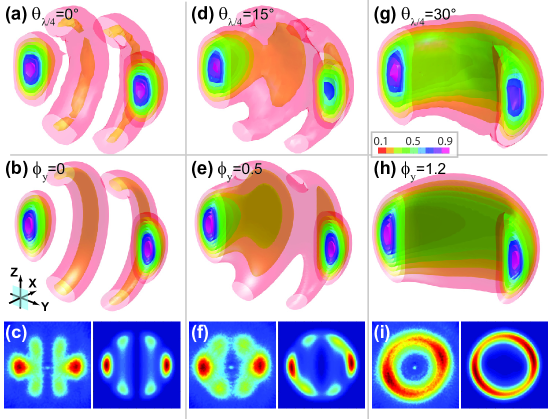
Figure 7: Comparison of calculated & experimental tomographic results. Panels show (top) experimental and (middle) calculated 3D distributions plotted as intensity iso-surfaces. The experimental data is plotted with a radial mask to show only the main part of the radial distribution. (Bottom) Experimental and calculated 2D projected images in the plane of polarization $(X,Y)$. In this case no radial mask is included in the experimental results, and the images show an extended energy range relative to the computational results (the broader spectrum is due to the presence of Autler-Townes splitting in this case, see main text for details). Columns show the results for different laser polarization states, defined by a quarter-wave plate rotation angle ($\theta_{\lambda/4}$) in the experimental data, and spectral phase $\phi_{y}$ in the calculations. The states correspond to ellipticities $\varepsilon\backsimeq$0, 0.3 and 0.6 (see ref. Hockett2015b for further details).

A qualitative comparison of data for the three different polarization states measured is presented in figure 7. In this figure the full 3D distributions are shown as nested iso-surface plots, and 2D images in the polarization plane are also shown. In this case, the experimental data has an additional high-energy feature in the radial distribution, arising from Autler-Townes splitting which becomes significant at higher intensities (see refs. Wollenhaupt2005b ; Wollenhaupt2009a , and ref. Hockett2015b ). In this analysis only the main feature is of interest, and the tomographic distributions shown include a radial mask in order to remove the additional contributions and facilitate comparison over the main spectral feature. For the 2D images (bottom row of fig. 7) no radial mask is employed and, consequently, the experimental results show a broadening of the spectrum in the 2D images. Full details of the experimental data and tomographic reconstruction procedure, as well as the energy spectra, are discussed in ref. Hockett2015b . It is also of note that the data shown in panels (a) and (d) of figure 7 are the same as shown in figure 3 of ref. Hockett2014 .

It is clear from figure 7 that the experimental data and the calculations agree in overall form, with the trend in the shape of the PADs with polarization well-reproduced by theory. This general behaviour is not surprising, since this sensitivity was inherent in the concept of obtaining the photoionization matrix elements via a fitting procedure from the 2D images recorded with different polarizations, but does indicate that the additional details observable in the tomographic data do not contradict the fit results, even at higher intensities which do affect the energy spectrum.

The 2D images appear to show less satisfactory agreement but, since these $(X,Y)$ plane projections include summation over the $Z$-axis, this is perhaps unsurprising. In particular, the apparent increase in intensity of the band structures in panel (c), relative to the computational results, is due to the additional (and incoherent) contribution from photoelectrons at different energies, due to the projection of the broader spectrum onto the 2D plane, and which are not present in the computational results. The most significant differences are seen in panel (f), where the asymmetry in the $(X,Y)$ plane - the helicity of the distribution - is reduced relative to the computational results. This is likely due to a slight difference of the polarization ellipse relative to the calculations, as well as the summation over the broader spectrum (as mentioned above) which may wash-out fine details in the projection image. For the results approaching circular polarization, panel (i), the agreement is better. In this case the contributions from the higher-energy AT feature are reduced (see ref. Hockett2015b ), and the polarization state of the light may be slightly better matched to that assumed in the calculation.

Overall these results indicate reasonably good agreement between the previously determined matrix elements and the tomographic data, but also indicate the problematic aspects of a qualitative comparison for these complex distributions. In general such comparisons are worthwhile, but subject to perceptual bias which may be highly dependent on the type of data visualization used. Naturally a quantitative comparison is preferable, and is explored in the following section.

IV.2 Quantitative comparison

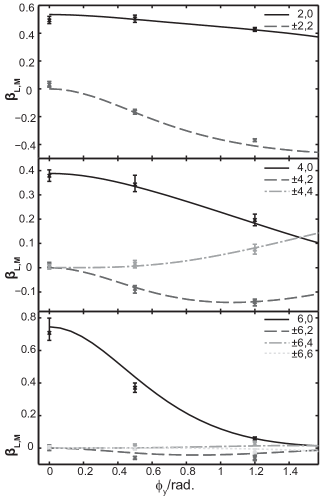
Figure 8: Comparison of calculated $\beta_{LM}^{k}$ (lines) and experimental results (crosses with error bars) as a function of polarization state. Panels show $L=2,\,4,\,6$, and line-styles and shade denote $M$. The error bars on the experimental results show the spread of $\beta_{L,M}(k)$ obtained over the FWHM of the main spectral feature.

To make a more careful comparison of the volumetric results, $\beta_{L,M}(k)$ were extracted from the data (see ref. Hockett2015b for details). The $\beta_{L,M}(k)$ over the main feature can then be directly compared with the predicted $\beta_{L,M}^{k}$ based on the fitted matrix elements. Since the fit results assume that the matrix elements are approximately constant over the feature, the experimental $\beta_{L,M}(k)$ were averaged over the FWHM of the main spectral feature to yield an energy-averaged value. These values are plotted in figure 8 along with the calculation results. The range of the experimental $\beta_{L,M}(k)$ are indicated by the error bars on the plot, indicating the spread of values over the spectrum.

The agreement between the calculation and experimental results is generally very good, if not exact. The dominant terms, with $L=2,\,4,\,6$ and $M=0$, show excellent agreement and, aside from $\beta_{6,0}$ at $\phi_{y}=0$, the experimental results also show only a small spread of values. For the $M\neq 0$ terms, which generally have smaller magnitudes than the $M=0$ terms except at large $\phi_{y}$, the agreement is generally good, but less so for the $|M|=2$ terms. Here the trends with polarization are in agreement, but the exact values are shifted slightly from the calculations. As noted above, these small discrepancies may be due to slight differences in the laser polarization and frame rotations used in the calculations as compared with the experiment.

Additionally, the experimental data indicated a significant energy-dependence of the PADs away from the main spectral feature, small contributions from higher-order terms ($L>6$) and symmetry breaking were also present. These effects are not accounted for by the net 3-photon model, and indicate the presence of additional complexities to the light-matter interaction. These additional effects are, at this time, not well-understood beyond the clear requirement for $\pm m$-state symmetry breaking, and for higher angular momentum states to be accessed. These observations are discussed further in ref. Hockett2015b , and it is of note that the ability to resolve these additional effects via the quantitative analysis of 3D photoelectron data is a significant outcome.

Despite these additional, but intriguing, complexities, the major channels observed over the FWHM of the main spectral feature are seen to agree very well with the previous analysis, based on 2D data recorded at lower intensities, overall providing a strong test of the accuracy of the ionization matrix elements determined in that case. The possibility of gaining a detailed understanding of the additional effects observed in the 3D data, starting from the current 3-photon model, and associated ionization matrix elements, remains an interesting proposition for future work. In the following section we explore some extensions to our treatment which may facilitate such understanding.

V Assumptions, extensions & physical considerations

In the above treatment, as applied in ref. Hockett2014 , some simplifications have been made for the specific case at hand, in order to facilitate the determination of the $R_{ll}(k)$ as detailed above (sect. III). Here, in order to generalize this treatment further, we consider more carefully the assumptions made and explore other extensions to the theory.

V.1 Atoms

The intra-pulse dynamics above implicitly assume that only the outermost electrons play a role in the intra-pulse dynamics, and that lower-lying bound states can be neglected. Furthermore, it assumes that the 4$p$ manifold is the only unpopulated state which plays a role at the 1-photon level. This is expected in this case because the 4$s\rightarrow$4$p$ transition carries significant oscillator strength, and is near resonant with the laser pulse. However, in general it is possible that other states will play a role, particularly as the laser is tuned further from the 4$s\rightarrow$4$p$ line. This would result in a more complex TDSE (eqn. 6), with additional states appearing, and also necessitate a more careful treatment of the transition dipoles $\mu_{L/R}$ to allow for variation in the transition amplitudes to different $|n,l\rangle$-manifolds. The treatment of the 2-photon ionization would, similarly, increase in complexity with the addition of further initial/source $|n,l\rangle$-manifolds, but would otherwise remain identical.

In the case of atomic ionization with a structureless continuum, the photoelectron energy spectrum can be treated somewhat directly as determined from the power spectral density of the laser pulse Wollenhaupt2002 ; Wollenhaupt2005 ; Wollenhaupt2009a . Such treatment effectively introduces an additional time-dependent phase into eqn. 8. In ref. Wollenhaupt2009a this phase is defined as $e^{i\delta\omega_{e}t}$, with $\delta\omega_{e}=\omega_{e}+\omega_{IP}-\omega_{p}-2\omega_{0}$, where the angular frequencies are related to the electron energy ($\hbar\omega_{e}$), the ionization potential ($\hbar\omega_{IP}$), the ionizing 4$p$ state ($\hbar\omega_{p}$) and the photon energy ($\hbar\omega_{0}$). This phase will thus oscillate rapidly at the resultant difference frequency of these terms (effectively the difference between the total final state energy and the incident/input energy), and directly gives rise to a photoelectron energy spectrum dependent on the pulse properties, including its temporal duration and structure Wollenhaupt2006 . This dependence can be considered interferometrically, in the sense that the resultant (time-integrated) energy spectrum is the coherent temporal sum, hence contains interferences between all instantaneous momentum distributions; this is exactly analogous to the PADs considered as the coherent temporal sum of the instantaneous angular distributions (at a given energy). In the case of pulses intense enough to create significant Autler-Townes splitting in the photoelectron energy spectrum, this treatment could allow for a description of the changes in the PADs and symmetry breaking, as discussed in sect. IV.2 and correlated with the Autler-Townes doublet in the spectrum. This consideration is discussed further in ref. Hockett2015b .

In the most general case, where multiple, non-degenerate ionization pathways may be present, interferences may arise between ionizing transitions with very different angular structures. In the energy domain this effect has been investigated by Elliott and co-workers in experiments utilizing fundamental and second-harmonic light to create final-state interferences between different intermediates Yin1992 ; Yin1995 ; Wang2001 . Control over the relative phase of the two colours allowed for control over the resultant interferences Yin1995 . A similar concept was also employed to measure the phase of a bound-state Fiss2000 . Practically, this most general effect could be included in our formalism by the inclusion of sets of ionization matrix elements correlated with the distinct sets of ionization pathways, where each set has a characteristic partial wave distribution (amplitudes and phases) and energy-dependent phase factor, and would result in the inclusion of interferences dependent on both geometric and energetic phase factors. Conceptually, this effect is inherent in the PADs arising from polarization shaped pulses, where the different ionization pathways correspond to different intermediate angular momentum states, but in this case all levels are degenerate and the relevant phase shifts are purely geometric.

V.2 Molecules

In the case of molecular ionization the situation is more complex. In this case, the partitioning of the incident photon angular momentum to molecular rotations, as well as the outgoing photoelectron, requires a more involved treatment of the geometric terms, even in a single active electron picture. Furthermore, one might expect that the continuum also contains structure due to population of different vibrational modes of the ion, although it is also possible that these states have little effect on the $R(k)$ integrals over a small energy range. This assumption formally means a separation of the ionization matrix element into electronic, vibrational (Franck-Condon) and rotational terms is possible, and that these terms are thus uncoupled. Effectively the electronic terms define the $R(k)$, and the Franck-Condon factors an overall transition intensity envelope - but one that does not affect the partial wave character of the continuum. In some cases this approximation has been tested, and found to hold, but in other cases - particularly when considering highly excited vibrational modes - one might expect this assumption to fail Lucchese2010 ; Lopez-Dominguez2012 .

In previous work we have investigated molecular ionization via vibrational and rotational state-resolved energy-domain experiments Hockett2007 ; Hockett2009 ; Hockett2010 ; Hockett2010a . This work demonstrates the feasibility of performing such experiments, and illustrates the types of angular momentum coupling schemes required. Although the current work, incorporating intra-pulse dynamics and polarization shaped pulses, has not yet been extended to molecular cases, such an extension seems feasible based on these earlier studies, at least from the perspective of treating the ionization matrix elements, and including the larger number of continuum $l$-waves required for molecular scattering problems.

The intra-pulse dynamics in the molecular case may, however, be significantly more challenging. Clearly there are many more degrees of freedom to account for, and the potential for both nuclear and electronic wavepacket motion during the pulse, as well as the possibility of dumping a lot of angular momentum into forming a rotational wavepacket during a strongly-coupled initial step (although the evolution of this wavepacket will ultimately be on a much slower timescale). The incorporation of such coupled rovibronic dynamics is, in practice, quite difficult due to the high-dimensionality of the problem. It is certainly not sufficient to perform a simple TDSE of coupled electronic states as employed herein, although the coupling of more complex wavepacket calculations with the ionization treatment herein would be feasible. A conceptually similar, although fully ab initio, coupling of complex vibronic wavepackets with a full photoionization calculation has recently been presented for the triatomic molecule CS₂ Wang2014 ; prior to this ab initio treatment a simpler dynamical model was combined with the relevant angular momentum coupling and gave good agreement with experimental results, although the treatment was only semi-quantitative and stopped short of extraction of the ionization matrix elements Hockett2011 . For diatomics it is probable that a conceptual middle-ground is found, in which the required low-dimensionality wavepacket can be modelled via a simple TDSE treatment with enough accuracy to be of use. For polyatomics, the complexity of the wavepacket will be the deciding factor, depending directly on the number and type of states and couplings involved in a given case. In the most complex cases the problem may be best treated by fully ab initio calculations including photoionization, the results of which can be compared directly with experimental data at a high level, but in simpler wavepackets (few level and/or weakly coupled) a basic TDSE approach may be of sufficient accuracy to be useful for complete experiments.

In sum, based on experience of similar problems in molecular ionization in both the energy and time domains, it seems feasible that this time-domain multiplexing concept, employing multi-photon ionization schemes, and with the inclusion of intra-pulse dynamics, can also be applied successfully to (at least some) molecular photoionization problems.

V.3 Other regimes

Other regimes are also of general interest in photoionization studies Reid2003 , in particular the strong-field (non-perturbative) regime. Very generally, the treatment presented herein could be extended to this regime, and the issues associated closely follow the discussion above. In the non-perturbative case the intra-pulse dynamics become more complicated, since a single-active electron picture is no longer likely to be valid, and a static picture of the bound state energy-level structure also breaks down. Similarly, the scattering dynamics of the outgoing electron will also be time-dependent, since the scattering must now incorporate the laser-induced part of the potential, not just the (static) atomic or molecular potential.

In theory it is feasible to allow for these effects into the treatment presented herein, since it is already time-dependent and, as discussed for the atomic and molecular cases above, additional dynamical effects could be readily incorporated providing the numerics are tractable and accurate. However, the main issue in terms of determining the ionization matrix elements would be the large size of the set of matrix elements to be determined in a fully time-dependent treatment and the concomitant complexity of the fitting procedure if a set of ionization matrix elements were required for each time-step. In such cases it may be possible to posit an effective functional dependence of the ionization dynamics on the laser field to mitigate this somewhat, but one would have to more carefully consider exactly what kind of measurement would allow for a unique set of (fitted) matrix elements to be extracted from the (necessarily) time-integrated photoelectron image.

Another regime is that of high-order light-matter couplings beyond the dipole approximation. In this case the ionization matrix elements contain higher-order angular momentum couplings, hence a more complex angular-momentum coupling scheme and a larger set of matrix elements must be determined, similar to the considerations for the molecular case. As for that case, there is no fundamental reason why such cases could not be treated within the theoretical framework presented here, although the feasibility of the fitting procedure would have to be assessed for any given case based on the size of the problem.

Another interesting extension is to ionization time delays, since the the Wigner delay time is given by the energy-derivative of the scattering phase Wigner1955 ; DeCarvalho2002 . Measurements of this phase, based on the concept of interfering photoelectron wavepackets created with different energies, have recently been demonstrated Klunder2011 ; Dahlstrom2012 and are very similar to to concepts herein. In such measurements, above-threshold ionization creates electron wavepackets at different energies (i.e. multiple spectral features in the photoelectron spectrum), and further photo-absorption from a probe laser field can be used to interfere neighbouring wavepackets. This procedure results in side-band generation in the photoelectron spectrum, and the phase of the oscillation of these side-bands with respect to the probe field timing provides information on the relative phase of the photoelectron wavepackets - this is know as the RABBITT technique Muller2002 ; Dahlstrom2012 (this concept is somewhat analogous to the two-pulse photoelectron interferometry of ref. Wollenhaupt2002 ). The difference between this concept and traditional “complete” photoionization experiments is that the total photoionization phase is measured over a broad energy spectrum in RABBITT measurements, as opposed to the measurement of the phases of the partial-waves at a single energy as discussed herein. By extending our technique to a broad energy range, e.g. via observation of multiple ATI features or the use of a broader bandwidth probe pulse, we would be able to obtain the partial-wave phases as a function of energy and, thus, determine the Wigner delay. Furthermore, by obtaining the phases for all partial-waves, the angle-dependence of the Wigner delay in molecular ionization could also be investigated Hockett2015c .

V.4 Maximum information measurements & multiplexing

In all cases discussed above, the main consideration is the feasibility of performing complete experiments for more complex, dynamical ionization schemes. Such applications will, naturally, be challenging, and require both a detailed theoretical understanding of the dynamics at hand and high-information experimental measurements. The majority of this work has focussed on assessing the results obtained for pure polarization states, in which there is no additional information gained from the coherent time-domain integration over the laser pulse, but for more complex cases the additional information content of polarization-multiplex measurements may be vital. Specifically, multiplexing provides additional time-domain interferences in the PADs (see eqn. 18), with the result that time-integrated polarization-multiplexed measurements contain the information of multiple pure-state measurements.

One particularly powerful aspect of using shaped pulses is the possibility of tailor-made pulses for metrology, designed to create or amplify specific interfering channels of interest. Conceptually this is identical to the use of shaped pulses for control Wollenhaupt2005 ; Wollenhaupt2009a , however the pulses would be designed for the purposes of obtaining detailed information on specific ionization channels, rather than for the purposes of creating a specific photoelectron distribution. The examples shown in figure 1 and 2 indicate how this concept operates: there are different continuum populations created in the two cases, the time-domain structure is more complex in the shaped pulse case and, most generally, the pulse shape can be chosen to select certain ionization channels (within the constraints imposed by the dynamics of the ionizing system). As well as polarization-shaping, the coherent time-domain treatment may also provide a way to probe additional intereferences due to effects such as intensity-dependent ionization phases. The presence of such effects at higher intensities has been determined from the behaviour of the PADs over the Autler-Townes structure of the photoelectron spectrum, as mentioned above (sect. IV.2), but remains to be understood in detail.

In all these cases, the PADs will usually be non-cyclindrically symmetric, so use of “maximum information measurements” utilizing 3D measurements and detailed analysis will also be required. The power of this approach has been touched on here, and is further explored in ref. Hockett2015b ; recent work has also considered 3D photoelectron measurements in the context of photoelectron circular dichroism Lux2015 .

VI Summary & conclusions

In this work the validity of a fitting approach to complete photoionization experiments in the multiphoton regime, incorporating intra-pulse dynamics, as initially reported in ref. Hockett2014 , has been explored. The details of the fitting procedure, based on statistical sampling of the $\chi^{2}$ hyperspace and further testing and validation of the results, were outlined as a pragmatic fitting methodology. The results presented in ref. Hockett2014 were discussed in detail, and compared both qualitatively and quantitatively with full 3D experimental photoelectron distributions. Finally, extension of this treatment to more complex ionization processes was discussed in general terms.

This analysis indicated the validity of the results already presented, as well as insight into the practicalities of a pragmatic fitting approach. Although this approach has yet to be tested beyond the use of pure polarization states, the use of polarization shaped pulses clearly offers an enhanced photoelectron metrology, with the possibility of controlling the information content via the pulse shape, as discussed in sect. II (see also ref. Hockett2014 ). The use of full 3D experimental measurements is another powerful aid to maximum information metrology, as indicated herein by comparison of the computational results with tomographically reconstructed experimental distributions (see also ref. Hockett2015b ). In general, we anticipate that the combination of these tools represents a powerful methodology for complete photoionization studies, or other research making use of ionization measurements.

Acknowledgement: Financial support by the State Initiative for the Development of Scientific and Economic Excellence (LOEWE) in the LOEWE-Focus ELCH is gratefully acknowledged.

References

- [1] Katharine L. Reid. Photoelectron angular distributions. Annual Review of Physical Chemistry, 54(1):397–424, 2003.
- [2] N.A. Cherepkov. Complete experiments in photoionization of atoms and molecules. Journal of Electron Spectroscopy and Related Phenomena, 144-147:1197 – 1201, 2005.
- [3] D Dill. Fixed-molecule photoelectron angular distributions. The Journal of Chemical Physics, 65(3):1130 – 1133, 1976.
- [4] P Lambropoulos. Using polarization effects in multiphoton ionization to measure ratios of bound-free matrix elements. Journal of Physics B: Atomic and Molecular Physics, 6(11):L319–L321, November 1973.
- [5] J. A. Duncanson, M. P. Strand, A. Lindgård, and R. S. Berry. Angular distributions of electrons from resonant two-photon ionization of sodium. Physical Review Letters, 37(15):987–990, Oct 1976.
- [6] H T Duong, J Pinard, and J L Vialle. Experimental separation and study of the two partial photoionisation cross sections 3p,s and 3p,d from the 3p state of sodium. Journal of Physics B: Atomic and Molecular Physics, 11(5):797–803, March 1978.
- [7] John Hansen, John Duncanson, Ring-Ling Chien, and R. S. Berry. Angular distributions of photoelectrons from resonant two-photon ionization of sodium through the 3p 0^{2}P_{3/2} intermediate state. Physical Review A, 21(1):222–233, January 1980.
- [8] Ring-ling Chien, Oliver Mullins, and R. Berry. Angular distributions and quantum beats of photoelectrons from resonant two-photon ionization of lithium. Physical Review A, 28(4):2078–2084, October 1983.
- [9] David J. Leahy, Katharine L. Reid, and Richard N. Zare. Complete description of two-photon (1+1[script ’]) ionization of no deduced from rotationally resolved photoelectron angular distributions. The Journal of Chemical Physics, 95(3):1757–1767, 1991.
- [10] Katharine L. Reid, David J. Leahy, and Richard N. Zare. Complete description of molecular photoionization from circular dichroism of rotationally resolved photoelectron angular distributions. Physical Review Letters, 68(24):3527–3530, Jun 1992.
- [11] Toshinori Suzuki. Femtosecond time-resolved photoelectron imaging. Annual review of physical chemistry, 57:555–92, January 2006.
- [12] Paul Hockett, Michael Staniforth, Katharine L. Reid, and Dave Townsend. Rotationally resolved photoelectron angular distributions from a nonlinear polyatomic molecule. Physical Review Letters, 102(25):253002, Jun 2009.
- [13] Yoshi-Ichi Suzuki, Ying Tang, and Toshinori Suzuki. Time-energy mapping of photoelectron angular distribution: application to photoionization stereodynamics of nitric oxide. Physical chemistry chemical physics : PCCP, 14(20):7309–20, May 2012.
- [14] O. Geßner, Y. Hikosaka, B. Zimmermann, A. Hempelmann, R. R. Lucchese, J. H. D. Eland, P.-M. Guyon, and U. Becker. inner valence photoionization dynamics of no derived from photoelectron-photoion angular correlations. Physical Review Letters, 88(19):193002, Apr 2002.
- [15] M. Lebech, J. C. Houver, A. Lafosse, D. Dowek, C. Alcaraz, L. Nahon, and R. R. Lucchese. Complete description of linear molecule photoionization achieved by vector correlations using the light of a single circular polarization. The Journal of Chemical Physics, 118(21):9653–9663, 2003.
- [16] Akira Yagishita, Kouichi Hosaka, and Jun-Ichi Adachi. Photoelectron angular distributions from fixed-in-space molecules. Journal of Electron Spectroscopy and Related Phenomena, 142(3):295 – 312, 2005.
- [17] P. Hockett, M. Wollenhaupt, C. Lux, and T. Baumert. Complete Photoionization Experiments via Ultrafast Coherent Control with Polarization Multiplexing. Physical Review Letters, 112(22):223001, June 2014.
- [18] Paul Hockett, Christian Lux, Matthias Wollenhaupt, and Thomas Baumert. Maximum information photoelectron metrology. In preparation, 2015.
- [19] Jean-Claude Diels and Wolfgang Rudolph. Ultrashort Laser Pulse Phenomena. Academic Press, Oxford, UK, second edition edition, 2006.
- [20] M. Wollenhaupt, M. Krug, J. Köhler, T. Bayer, C. Sarpe-Tudoran, and T. Baumert. Photoelectron angular distributions from strong-field coherent electronic excitation. Applied Physics B, 95(2):245–259, February 2009.
- [21] For completeness we note that in the presence of resonances at the 1-photon level, the bound-bound transitions would look identical within a single active electron model, apart from taking on specific, well-defined values of . In the case where several resonant states, e.g. high-lying Rydbergs, were within the laser bandwidth the dependence of the magnitudes and phases on would be significant. Pertinent examples of this type of effect in a multi-photon ionization scheme can be found in refs. [56, 57].
- [22] Hongkun Park and Richard N. Zare. Molecular-orbital decomposition of the ionization continuum for a diatomic molecule by angle- and energy-resolved photoelectron spectroscopy. I. Formalism. The Journal of Chemical Physics, 104(12):4554, 1996.
- [23] C. Yang. On the Angular Distribution in Nuclear Reactions and Coincidence Measurements. Physical Review, 74(7):764–772, October 1948.
- [24] R E Continetti. Coincidence spectroscopy. Annual review of physical chemistry, 52:165–92, January 2001.
- [25] Katharine L. Reid. Photoelectron angular distributions: developments in applications to isolated molecular systems. Molecular Physics, 110(3):131–147, February 2012.
- [26] Paul Hockett, Enrico Ripani, Andrew Rytwinski, and Albert Stolow. Probing ultrafast dynamics with time-resolved multi-dimensional coincidence imaging: butadiene. Journal of Modern Optics, 60(17):1409–1425, October 2013.
- [27] M. Wollenhaupt, M. Krug, J. Köhler, T. Bayer, C. Sarpe-Tudoran, and T. Baumert. Three-dimensional tomographic reconstruction of ultrashort free electron wave packets. Applied Physics B, 95(4):647–651, April 2009.
- [28] C Smeenk, L Arissian, a Staudte, D M Villeneuve, and P B Corkum. Momentum space tomographic imaging of photoelectrons. Journal of Physics B: Atomic, Molecular and Optical Physics, 42(18):185402, September 2009.
- [29] Paul Hockett, Michael Staniforth, and Katharine L. Reid. Photoelectron angular distributions from rotationally state-selected NH 3 (B 1 E"): dependence on ion rotational state and polarization geometry. Molecular Physics, 108(7-9):1045–1054, April 2010.
- [30] M. Wollenhaupt, a. Assion, D. Liese, Ch. Sarpe-Tudoran, T. Baumert, S. Zamith, M. Bouchene, B. Girard, a. Flettner, U. Weichmann, and G. Gerber. Interferences of Ultrashort Free Electron Wave Packets. Physical Review Letters, 89(17):1–4, October 2002.
- [31] Matthias Wollenhaupt, Christian Lux, Marc Krug, and Thomas Baumert. Tomographic reconstruction of designer free-electron wave packets. Chemphyschem : a European journal of chemical physics and physical chemistry, 14(7):1341–9, May 2013.
- [32] Paul Hockett. Photoionization Dynamics of Polyatomic Molecules. PhD thesis, University of Nottingham, 2009.
- [33] In this case parameters to allow for rotation of the image in the detector plane were not included, but in general could also be included.
- [34] Philip R. Bevington and D. Keith Robinson. Data Reduction and Error Analysis for the Physical Sciences. McGraw-Hill, New York, 2nd edition, 1992.
- [35] B Schmidtke, M Drescher, N a Cherepkov, and U Heinzmann. On the impossibility to perform a complete valence-shell photoionization experiment with closed-shell atoms. Journal of Physics B: Atomic, Molecular and Optical Physics, 33(13):2451–2465, July 2000.
- [36] M Wollenhaupt, A Präkelt, C Sarpe-Tudoran, D Liese, and T Baumert. Strong field quantum control by selective population of dressed states. Journal of Optics B: Quantum and Semiclassical Optics, 7(10):S270–S276, October 2005.
- [37] M Wollenhaupt, V Engel, and T Baumert. Femtosecond laser photoelectron spectroscopy on atoms and small molecules: prototype studies in quantum control. Annual review of physical chemistry, 56:25–56, January 2005.
- [38] M. Wollenhaupt, A. Präkelt, C. Sarpe-Tudoran, D. Liese, T. Bayer, and T. Baumert. Femtosecond strong-field quantum control with sinusoidally phase-modulated pulses. Physical Review A - Atomic, Molecular, and Optical Physics, 73(6):063409, June 2006.
- [39] Yi-Yian Yin, Ce Chen, D. S. Elliott, and A. V. Smith. Asymmetric photoelectron angular distributions from interfering photoionization processes. Physical Review Letters, 69(16):2353–2356, Oct 1992.
- [40] Yi-Yian Yin, D. S. Elliott, R. Shehadeh, and E. R. Grant. Two-pathway coherent control of photoelectron angular distributions in molecular no. Chemical Physics Letters, 241(5-6):591 – 596, 1995.
- [41] Zheng-Min Wang and D. S. Elliott. Determination of the phase difference between even and odd continuum wave functions in atoms through quantum interference measurements. Physical Review Letters, 87(17):173001, Oct 2001.
- [42] Ja Fiss, a Khachatrian, K Truhins, L Zhu, Rj Gordon, and T Seideman. Direct observation of a breit-wigner phase of a wave function. Physical review letters, 85(10):2096–9, September 2000.
- [43] Robert R. Lucchese, Raffaele Montuoro, Konstantinos Kotsis, Motomichi Tashiro, Masahiro Ehara, John D. Bozek, Aloke Das, April Landry, Jeff Rathbone, and E.D. Poliakoff. The effect of vibrational motion on the dynamics of shape resonant photoionization of BF 3 leading to the state of. Molecular Physics, 108(7-9):1055–1067, April 2010.
- [44] J.a. López-Domínguez, David Hardy, Aloke Das, E.D. Poliakoff, Alex Aguilar, and Robert R. Lucchese. Mechanisms of Franck-Condon breakdown over a broad energy range in the valence photoionization of N2 and CO. Journal of Electron Spectroscopy and Related Phenomena, 185(8-9):211–218, September 2012.
- [45] Paul Hockett and Katharine L Reid. Complete determination of the photoionization dynamics of a polyatomic molecule. II. Determination of radial dipole matrix elements and phases from experimental photoelectron angular distributions from A1Au acetylene. The Journal of chemical physics, 127(15):154308, October 2007.
- [46] Paul Hockett, Michael Staniforth, and Katharine L Reid. Photoionization dynamics of ammonia (B(1)E”): dependence on ionizing photon energy and initial vibrational level. The journal of physical chemistry. A, 114(42):11330–6, October 2010.
- [47] Kwanghsi Wang, Vincent McKoy, Paul Hockett, and Michael S. Schuurman. Time-Resolved Photoelectron Spectra of CS2: Dynamics at Conical Intersections. Physical Review Letters, 112(11):113007, March 2014.
- [48] Paul Hockett, Christer Z. Bisgaard, Owen J. Clarkin, and Albert Stolow. Time-resolved imaging of purely valence-electron dynamics during a chemical reaction. Nature Physics, 7(8):612–615, April 2011.
- [49] Eugene Wigner. Lower Limit for the Energy Derivative of the Scattering Phase Shift. Physical Review, 98(1):145–147, April 1955.
- [50] C.A.A. de Carvalho and H.M. Nussenzveig. Time delay. Physics Reports, 364(2):83–174, June 2002.
- [51] K. Klünder, J. M. Dahlström, M. Gisselbrecht, T. Fordell, M. Swoboda, D. Guénot, P. Johnsson, J. Caillat, J. Mauritsson, A. Maquet, R. Taïeb, and A. L’Huillier. Probing Single-Photon Ionization on the Attosecond Time Scale. Physical Review Letters, 106(14):1–4, April 2011.
- [52] J M Dahlström, A L’Huillier, and A Maquet. Introduction to attosecond delays in photoionization. Journal of Physics B: Atomic, Molecular and Optical Physics, 45(18):183001, September 2012.
- [53] H. G. Muller. Reconstruction of attosecond harmonic beating by interference of two-photon transitions. Applied Physics B: Lasers and Optics, 74:17–21, 2002.
- [54] Paul Hockett, Eugene Frumker, David M Villeneuve, and Paul B Corkum. Time delay in molecular photoionization. In preparation, 2015.
- [55] Christian Lux, Matthias Wollenhaupt, Cristian Sarpe, and Thomas Baumert. Photoelectron Circular Dichroism of Bicyclic Ketones from Multiphoton Ionization with Femtosecond Laser Pulses. ChemPhysChem, 16(1):115–137, January 2015.
- [56] M Krug, T Bayer, M Wollenhaupt, C Sarpe-Tudoran, T Baumert, S S Ivanov, and N V Vitanov. Coherent strong-field control of multiple states by a single chirped femtosecond laser pulse. New Journal of Physics, 11(10):105051, October 2009.
- [57] Iain Wilkinson, Andrey E Boguslavskiy, Jochen Mikosch, Julien B Bertrand, Hans Jakob Wörner, David M Villeneuve, Michael Spanner, Serguei Patchkovskii, and Albert Stolow. Excited state dynamics in SO2. I. Bound state relaxation studied by time-resolved photoelectron-photoion coincidence spectroscopy. The Journal of chemical physics, 140(20):204301, May 2014.