Nonlinear mechanisms to Rogue events in the process of interaction between optical filaments

Abstract

We investigate two types of nonlinear interaction between collinear femtosecond laser pulses with power slightly above the critical for self-focusing $P_{cr}$. In the first case we study energy exchange between filaments. The model describes this process through degenerate four-photon parametric mixing (FPPM) scheme and requests initial phase difference between the waves. When there are no initial phase difference between the pulses, the FPPM process does not work. In this case it is obtained the second type of interaction as merging between two, three or four filaments in a single filament with higher power. It is found that in the second case the interflow between the filaments has potential of interaction due to cross-phase modulation (CPM).

I Introduction

When two, three, four or higher number of filaments propagate in parallel and close trajectories, interflow and observation of extreme events are reported TZ ; KOZ ; CHEK ; SKUP ; WAH . These mergers, with appearing of a strong filament, were called Rogue events during the filamentation process. The coupling between two filaments was experimentally observed for first time in TZ . The conditions for optimal coupling were obtained later from Kosareva et al. KOZ and the optimum is for filaments with power near to critical for self-focusing and small diameter of the spot $r_{0}<3mm$. As it was reported recently in GAETA , depending on the relative phase and the incidence angle, the filament can experience fusion, repulsion, energy redistribution and spirial motion. The experiments in xenon gas were performed with several gigawatts input peak power SKUP to obtain parallel filament strings with numbers $N<12$. The laser pulse breaks up from spatially homogeneous beam profile into several highly localized filament strings each with pulse power slightly above the critical for self-focusing $P_{cr}$ BERGE ; BOYD . This is the reason to look for nonlinear optical mechanisms leading to exchange of energy or mergers during the process of multifilament propagation. The three dimensional localization appears similar to the soliton interaction in one-dimensional system as optical fibers, and based on clamping effects due to CPM MEN1 ; MEN2 ; KOV1 ; KOV2 and FPPM KOV2 . The nonlinear interaction process in fibers strongly depends on the initial phase difference between the pulses.

In this paper we propose a nonlinear vector model, where in details is investigated the role of CPM and degenerate FPPM processes in respect to the relative movements of laser filaments. We investigate numerically the interaction between optical pulses in the cases when: 1) the initial phase difference between pulses is not equal to zero $\Delta\varphi\neq 0$ and 2) the initial optical pulses admit equal phases $\Delta\varphi=0$. Thus, by properly selected initial conditions, we take into account the FPPM process as addition to the CPM influence. The proposed nonlinear vector model is investigated numerically on the base of the split-step Fourier method. We introduce by the moment formalism nonlinear acceleration and potentials between the weight centrums of the pulses.

II Theory: Nonlinear Polarization and basic system of equations

As it was pointed in KOL1 ; KOL2 ; KOVBOOK , the filamentation process can be described more correctly by using the generalized nonlinear operator

$$\vec{P}^{nl}=n_{2}\left(\vec{E}\cdot\vec{E}\right)\vec{E},$$ (1)

which includes additional processes associated with third harmonic generation. We substitute into the nonlinear operator (1) two-component electrical vector $\vec{E}=(E_{x},E_{y},0)$ at one carrying frequency $\omega_{0}$

$$\vec{E}=\frac{\left(A_{x}\exp\left[i(\omega_{0}t-k_{0}z)\right]+c.c.\right)}{2}\vec{x}+\frac{\left(A_{y}\exp\left[i(\omega_{0}t-k_{0}z)\right]+c.c.\right)}{2}\vec{y},$$ (2)

where $A_{x}=A_{x}(x,y,z,t),A_{y}=A_{y}(x,y,z,t)$ are the amplitude functions and $k_{0}$ is the carrying wave number of the laser source.

The nonlinear polarization (1) generates the following components

$$\vec{P}^{nl}_{x}=\tilde{n}_{2}\left[\frac{1}{3}\left(A_{x}^{2}+A_{y}^{2}\right)A_{x}\exp\left[2i(\omega_{0}t-k_{0}z)\right]+\left(|A_{x}|^{2}+\frac{2}{3}|A_{y}|^{2}\right)A_{x}+\frac{1}{3}A_{x}^{*}A_{y}^{2}\right]\exp\left[i(\omega_{0}t-k_{0}z)\right]+c.c.$$

(3)

$$\vec{P}^{nl}_{y}=\tilde{n}_{2}\left[\frac{1}{3}\left(A_{x}^{2}+A_{y}^{2}\right)A_{y}\exp\left[2i(\omega_{0}t-k_{0}z)\right]+\left(|A_{y}|^{2}+\frac{2}{3}|A_{x}|^{2}\right)A_{y}+\frac{1}{3}A_{y}^{*}A_{x}^{2}\right]\exp\left[i(\omega_{0}t-k_{0}z)\right]+c.c.,$$

where $\tilde{n}_{2}=\frac{3}{8}n_{2}$. The operator $n_{2}\left(\vec{E}\cdot\vec{E}\right)\vec{E}$ generalizes the case of Marker and Terhune’s operator, and includes to the self-action terms, CPM terms, FPPM terms and also additional terms associated with Third-Harmonic Generation (THG).

The initial laser pulses $\left(t_{0}\geq 50fs\right)$ possess a relatively narrow-band spectrum $\left(\Delta k_{z}\ll k_{0}\right)$ ($\Delta k_{z}$ is the spectral pulse width). During the filamentation process the initial self-focusing broadens significantly the pulse spectrum. The broad-band spectrum $\left(\Delta k_{z}\sim k_{0}\right)$ is one of the basic characteristics of the stable filament. The dynamics of broad-band pulses can be presented properly within different non-paraxial models such as UPPE KOL1 ; KOL2 or non-paraxial envelope equations KOVBOOK . Another standard restriction in the filamentation theory is the use of one-component scalar approximation of the electrical field $\vec{E}$. This approximation though, is in contradiction with recent experimental results, where rotation of the polarization vector is observed KOSA ; ZIG . For this reason, in the present paper we use the non-paraxial vector model up to second order of dispersion, in which the nonlinear effects are described by the nonlinear polarization components (II). The system of non-paraxial equations of the amplitude functions $A_{x},A_{y}$ of the two-component electrical field (2) has the form

$$-2i\frac{k_{0}}{v_{gr}}\frac{\partial A_{x}}{\partial t}=\Delta_{\bot}A_{x}-\frac{\beta+1}{v_{gr}}\left(\frac{\partial^{2}A_{x}}{\partial t^{2}}-2v_{gr}\frac{\partial^{2}A_{x}}{\partial t\partial z}\right)-\beta\frac{\partial^{2}A_{x}}{\partial z^{2}}$$

$$+k^{2}_{0}\tilde{n}_{2}\left[\frac{1}{3}\left(A^{2}_{x}+A^{2}_{y}\right)A_{x}\exp\left(2ik_{0}\left(z-\left(v_{ph}-v_{gr}\right)t\right)\right)+\left(|A_{x}|^{2}+\frac{2}{3}|A_{y}|^{2}\right)A_{x}+\frac{1}{3}A^{*}_{x}A^{2}_{y}\right]$$

(4)

$$-2i\frac{k_{0}}{v_{gr}}\frac{\partial A_{y}}{\partial t}=\Delta_{\bot}A_{y}-\frac{\beta+1}{v_{gr}}\left(\frac{\partial^{2}A_{y}}{\partial t^{2}}-2v_{gr}\frac{\partial^{2}A_{y}}{\partial t\partial z}\right)-\beta\frac{\partial^{2}A_{y}}{\partial z^{2}}$$

$$+k^{2}_{0}\tilde{n}_{2}\left[\frac{1}{3}\left(A^{2}_{x}+A^{2}_{y}\right)A_{y}\exp\left(2ik_{0}\left(z-\left(v_{ph}-v_{gr}\right)t\right)\right)+\left(|A_{y}|^{2}+\frac{2}{3}|A_{x}|^{2}\right)A_{y}+\frac{1}{3}A^{*}_{y}A^{2}_{x}\right],$$

where $v_{gr}$ and $v_{ph}$ are the group and phase velocities correspondingly, $\beta=k_{0}v_{gr}^{2}k^{\prime\prime}$ and $k^{\prime\prime}$ is the group velocity dispersion.

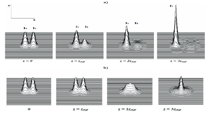
Figure 1: (1a) Energy exchange between two collinear filaments $\vec{A}_{1}$ and $\vec{A}_{2}$ with power slightly above the critical $P_{cr}$ ($\gamma=1.5$). The pulses are separated initially at distance $2a=3.4$ and the evolution is governed by the system of equations (II). In the initial conditions (III) the phase difference $\varphi=\pi/4$ correspond to maximal energy exchange. Due to degenerated FPPM process one of the filaments is amplified while the other filament enters in linear mode and vanishes. (1b) Fusion between the same pulses when they are with equal initial phases, i. e. $\Delta\varphi=0$. The similar picture is seen when the FPPM terms are excluded from the equations (II) and only interaction due to CPM is investigated. With $z_{diff}$ is denoted the diffraction length $z_{diff}=k_{0}r_{0}^{2}$.

This model describes the ionization-free filamentation regime, where the pulse intensities are close to the critical one for self-focusing. The first nonlinear term in (II) corresponds to coherent GHz generation KOVBOOK . The system (II) is written in Galilean frame $\left(z^{\prime}=z-vt;t^{\prime}=t\right)$. In all coordinate systems - laboratory, moving in time, and Galilean, the group velocity adds an additional phase (carrier-envelope phase) in the third harmonic terms and transforms them to GHz ones. This can be seen directly for the system (II) written in Galilean frame, which determines the choice of coordinates. The last nonlinear term in (II) describes degenerate four-photon parametric mixing. To satisfy the Manley-Rowe relations of the truncated equations with a generalized nonlinear polarization of the type $\vec{P}^{nl}=n_{2}\left(\vec{E}\cdot\vec{E}\right)\vec{E}$, some restrictions on the components of the electrical field are imposed. The condition is simple - the possible initial components $A_{x}$ and $A_{y}$ should be complex-conjugated fields. The conservation laws give us additional information on the behavior of the vector amplitude function: only components of the vector amplitude field $\vec{A}=(A_{x},A_{y},0)$, which present rotation of the vector $\vec{A}$ in the plane $(x,y)$, satisfy the MR conditions. That is why in our numerical experiments, as well as in our analytical investigations, we will use complex-conjugated components only.

The system of equations (II) written in dimensionless form becomes

$$-2i\alpha\delta^{2}\frac{\partial A_{x}}{\partial t}=\Delta_{\bot}A_{x}-\delta^{2}\left(\beta+1\right)\left(\frac{\partial^{2}A_{x}}{\partial t^{2}}-\frac{\partial^{2}A_{x}}{\partial t\partial z}\right)-\delta^{2}\beta\frac{\partial^{2}A_{x}}{\partial z^{2}}$$

$$+\gamma\left[\frac{1}{3}\left(A^{2}_{x}+A^{2}_{y}\right)A_{x}\exp\left(2i\alpha\left(z-\Delta\tilde{v}_{nl}t\right)\right)+\left(|A_{x}|^{2}+\frac{2}{3}|A_{y}|^{2}\right)A_{x}+\frac{1}{3}A^{*}_{x}A^{2}_{y}\right]$$

(5)

$$-2i\alpha\delta^{2}\frac{\partial A_{y}}{\partial t}=\Delta_{\bot}A_{y}-\delta^{2}\left(\beta+1\right)\left(\frac{\partial^{2}A_{y}}{\partial t^{2}}-\frac{\partial^{2}A_{y}}{\partial t\partial z}\right)-\delta^{2}\beta\frac{\partial^{2}A_{y}}{\partial z^{2}}$$

$$+\gamma\left[\frac{1}{3}\left(A^{2}_{x}+A^{2}_{y}\right)A_{y}\exp\left(2i\alpha\left(z-\Delta\tilde{v}_{nl}t\right)\right)+\left(|A_{y}|^{2}+\frac{2}{3}|A_{x}|^{2}\right)A_{y}+\frac{1}{3}A^{*}_{y}A^{2}_{x}\right],$$

where $x=x/r_{0}$, $y=y/r_{0}$, $z=z/r_{0}$ are the dimensionless coordinates, $r_{0}$ is the pulse waist, $z_{0}=v_{gr}t_{0}$ is the spatial pulse length, $\alpha=k_{0}z_{0}$, $\delta=r_{0}/z_{0}$, $\gamma=k^{2}_{0}r^{2}_{0}\tilde{n}_{2}|A_{0}|^{2}/2$ is the nonlinear coefficient and $\Delta\tilde{v}_{nl}=\left(v_{ph}-v_{gr}\right)/v_{gr}$ is the normalized group-phase velocity difference.

III Numerical simulations

In the experiments on multi-filamentation two basic trends are observed. The first one is that the number of filaments is reduced significantly as a function of the distance KILO . The second trend is observed recently in TZ ; KOZ ; CHEK ; SKUP ; WAH as mergers between two, tree or four filaments in one (Rogue) wave. We think that the both processes are connected and they are results of different types of nonlinear interaction. Therefore we investigated in details interaction of two filaments. By control of the initial phase difference between the pulses it is possible to include or exclude the process of FPPM in the nonlinear interaction. When the initial phase difference between the pulses is not equal to zero, the process of FPPM starts to work and an intensive exchange of energy is observed DAN . When the initial phase difference of the pulses is equal to zero the process of FPPM practically does not work and the nonlinear interaction is due the CPM process.

The numerical results are presented for initial conditions: $120fs$ Gaussian bullets with waist and spatial length $r_{0}=z_{0}=72\mu m$ and power slightly above $P_{cr}$. In this case $\alpha=90\pi$, $\delta=1$, $\Delta\tilde{v}_{nl}=0.00023$ and $\gamma\in 1.5-3$. The phase difference between the $A_{x}$ and $A_{y}$ components is initially $\pi/2$ in order to satisfy the conservation laws. We investigate two collinear laser pulses as two vector fields $\vec{A}_{1}$ and $\vec{A}_{2}$ at small distance $a$ between them. Each of the pulses admits $\vec{x}$ and $\vec{y}$ components: $\vec{A}_{j}=A_{j,x}\vec{x}+A_{j,y}\vec{y},j=1,2$. The initial conditions for numerical solution of the system of equations (II) have the form

$$A_{x}=A_{1,x}+A_{2,x}=\frac{A^{0}_{1}}{\sqrt{2}}\exp\left(-\frac{(x+a)^{2}+y^{2}+z^{2}}{2}\right)$$

$$+\frac{A^{0}_{2}}{\sqrt{2}}\exp\left(-\frac{(x-a)^{2}+y^{2}+z^{2}}{2}\right)\exp\left(i\Delta\varphi\right)$$

(6)

$$A_{y}=A_{1,y}+A_{2,y}=\Biggr{\{}\frac{A^{0}_{1}}{\sqrt{2}}\exp\left(-\frac{(x+a)^{2}+y^{2}+z^{2}}{2}\right)$$

$$+\frac{A^{0}_{2}}{\sqrt{2}}\exp\left(-\frac{(x-a)^{2}+y^{2}+z^{2}}{2}\right)\exp\left(i\Delta\varphi\right)\Biggr{\}}\exp\left(i\frac{\pi}{2}\right),$$

where $A_{x}$ and $A_{y}$ are composed of the $x$- and $y$-components of the two optical pulses propagating along different parallel trajectories. The phase difference between the $A_{x}$ and $A_{y}$ components is initially $\pi/2$ in order to satisfy the conservation laws, while the phase difference between the pulses is denoted by $\Delta\varphi$. By varying the phase difference $\Delta\varphi$ we include (and exclude, when $\Delta\varphi=0$) the FPPM process. The interaction of optical pulses $\vec{A}_{1}$ and $\vec{A}_{2}$ for $\gamma=1.5$, $\Delta v=1.5$, $2a=3.4$ and $\Delta\varphi=\pi/4$ is shown on Fig. 1a. It is observed that the amplified pulse self-focuses and gets enough power to continue its propagation, while the other pulse gives out energy, enters into linear mode and vanishes. In this way the number of filaments can be reduced by non-linear parametric processes in $\chi^{(3)}$ media. In the following numerical experiment (Fig. 1b) we exclude the FPPM process by using initial phase difference $\Delta\varphi=0$. To verify this result we also exclude the parametric step from the the system of equations (II) and increase the intensity by factor $1/4$ to keep on the critical power. The pulses start to attract each other without energy exchange and as result a merging and self-focusing are observed. In the both numerical experiments (with $\Delta\varphi=0$ or when the parametric step is excluded from the program) the results are similar - there is no energy exchange and the fusing between the filaments is clearly seen. Similar potential type of interaction by CPM was reported in optical fibers KOV1 ; KOV2 . In the following section of this paper we calculate the nonlinear acceleration and potential between the weight centers of optical pulses. In the general case of few optical filaments usually there are random phase differences between the waves. On Fig. 2 the interaction between three pulses is presented. Two of them are with equal initial phases, while the third one admits phase difference $\Delta\varphi=\pi/4$ in respect to others. Similar dependance on the initial phase difference is observed: fusion between the pulses with equal phases, while the third one exchanges energy by FPPM process.

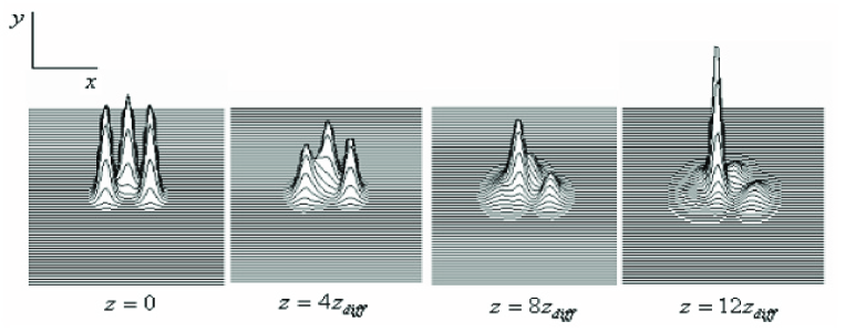
Figure 2: Interaction between three collinear filaments $\vec{A}_{1}$, $\vec{A}_{2}$ and $\vec{A}_{3}$ governed by the system of equations (II). Two of the pulses are with equal initial phases, while the third admits phase difference $\Delta\varphi=\pi/4$ in respect to others. Fusing between the pulses with equal phases is seen, while the third one exchanges energy by FPPM process.

IV Moment formalism and potentials

To obtain analytical expressions of the influence of CPM on the relative moving of optical pulses we exclude the FPPM process and GHz generation from the system of equations (II). The basic system in this case is transformed to $(3+1)D$ of Manakov type

$$-2ik_{0}\left[\frac{1}{v_{gr}}\frac{\partial A_{x}}{\partial t}+\frac{\partial A_{x}}{\partial z}\right]=\Delta A_{x}-\frac{1+k_{0}v_{gr}^{2}k^{{}^{\prime\prime}}}{v_{gr}^{2}}\frac{\partial^{2}A_{x}}{\partial t^{2}}+k^{2}_{0}\tilde{n}_{2}\left(|A_{x}|^{2}+\frac{2}{3}|A_{y}|^{2}\right)A_{x}$$

(7)

$$-2ik_{0}\left[\frac{1}{v_{gr}}\frac{\partial A_{y}}{\partial t}+\frac{\partial A_{y}}{\partial z}\right]=\Delta A_{y}-\frac{1+k_{0}v_{gr}^{2}k^{{}^{\prime\prime}}}{v_{gr}^{2}}\frac{\partial^{2}A_{y}}{\partial t^{2}}+k^{2}_{0}\tilde{n}_{2}\left(|A_{y}|^{2}+\frac{2}{3}|A_{x}|^{2}\right)A_{y}.$$

The scalar case of nonlinear interaction is investigated in KOV2 . In this paper we will preform similar analysis applied to collinear laser pulses presented as vector fields $\vec{A}_{1}$ and $\vec{A}_{2}$. We decompose as in the previous section the vectors $\vec{A}_{1}$ and $\vec{A}_{2}$ in $(x,y)$ plane

$$\vec{A}_{j}=A_{j,x}\vec{x}+A_{j,y}\vec{y};\,\,j=1,2.$$ (8)

Thus, the components $A_{x}$ and $A_{y}$ in (IV) become

$$A_{x}=A_{1,x}+A_{2,x};\,\,A_{y}=A_{1,y}+A_{2,y}.$$ (9)

Let us introduce the integral of energy of $A_{x}$ and $A_{y}$

$$p_{j}=\int\int\int|A_{j}\left(x,y,z,t\right)|^{2}\,dU=const;\,\,j=x,y$$ (10)

where $dU=dxdydz$ and also the integrals of center of weight in $x$ direction of $A_{x}$ and $A_{y}$ are

$$\left\langle X_{j}\right\rangle=\frac{1}{p_{j}}\int\int\int x|A_{j}\left(x,y,z,t\right)|^{2}\,dU;\,\,j=x,y,$$ (11)

Only the second derivative $\frac{\partial^{2}}{\partial x^{2}}$ in the system (IV) is non-commutative operator in regard to $x$ translation. The other differential operators commute with $x$ and therefore the velocity in $x$ direction of the center of weight can be written as

$$\left\langle\dot{X_{j}}\right\rangle=\frac{iv_{gr}}{2k_{0}p_{j}}\int\int\int\left[A_{j}^{*}\left(x,y,z,t\right)\frac{\partial A_{j}\left(x,y,z,t\right)}{\partial x}-A_{j}\left(x,y,z,t\right)\frac{\partial A_{j}^{*}\left(x,y,z,t\right)}{\partial x}\right]\,dU;\,\,j=x,y.$$ (12)

The acceleration in $x$ direction of the center of weight can be expressed by the following convolution integral

$$\left\langle\ddot{X_{j}}(\Delta x,t)\right\rangle=\frac{v_{gr}k_{0}\tilde{n}_{2}}{3p_{j}}\int\int\int\left[|A_{j}\left(x+\Delta x,y,z,t\right)|^{2}\frac{\partial}{\partial x}|A_{k}\left(x,y,z,t\right)|^{2}\right]\,dU;\,\,j=x,y,$$ (13)

where $k\neq j$. In the similar way we obtain the expressions of the accelerations in $y$ and $z$ directions. The total acceleration of the components $A_{x}$ and $A_{y}$ can be presented by the following vector sums

$$\left\langle\ddot{X_{j}}(\Delta x,t)\right\rangle\vec{x}+\left\langle\ddot{Y_{j}}(\Delta y,t)\right\rangle\vec{y}+\left\langle\ddot{Z_{j}}(\Delta z,t)\right\rangle\vec{z}=$$

$$\frac{v_{gr}k_{0}\tilde{n}_{2}}{3p_{i}}\int\int\int\left[|A_{j}\left(x+\Delta x,y+\Delta y,z+\Delta z,t\right)|^{2}\nabla|A_{k}\left(x,y,z,t\right)|^{2}\right]\,dU;\,\,j=x,y,$$ (14)

where with $\nabla=\partial/\partial x+\partial/\partial y+\partial/\partial z$ is denoted the gradient operator of the scalar field $|A_{k}\left(x,y,z,t\right)|^{2}$ and the expression under the integral is

$$|A_{j}\left(x+\Delta x,y+\Delta y,z+\Delta z,t\right)|^{2}\nabla|A_{k}\left(x,y,z,t\right)|^{2}=|A_{j}\left(x+\Delta x,y,z,t\right)|^{2}\frac{\partial(|A_{k}\left(x,y,z,t\right)|^{2})}{\partial x}+$$

$$|A_{j}\left(x,y+\Delta y,z,t\right)|^{2}\frac{\partial(|A_{k}\left(x,y,z,t\right)|^{2})}{\partial y}+|A_{j}\left(x,y,z+\Delta z,t\right)|^{2}\frac{\partial(|A_{k}\left(x,y,z,t\right)|^{2})}{\partial z};\,\,j=x,y.$$ (15)

Here we investigate the simplest case of two spherically-symmetric pulses, located at arbitrary distance $\Delta x$ in $x$ direction. Then, since $\Delta y=\Delta z=0$, the convolution integrals in $y$ and $z$ planes are equal to zero. Therefore we calculate the acceleration in $x$ direction (13) only. Substituting the decomposition (9) in (13) we obtain

$$\left\langle\ddot{a}(\Delta x,t)\right\rangle_{\vec{A}_{1}}=C_{1}\int\int\int\Bigg{[}|A_{x_{1}}\left(x+\Delta x,y,z,t\right)|^{2}\frac{\partial}{\partial x}|A_{y_{2}}\left(x,y,z,t\right)|^{2}+$$

$$+|A_{y_{1}}\left(x+\Delta x,y,z,t\right)|^{2}\frac{\partial}{\partial x}|A_{x_{2}}\left(x,y,z,t\right)|^{2}\Bigg{]}\,dU,$$ (16)

$$\left\langle\ddot{a}(\Delta x,t)\right\rangle_{\vec{A}_{2}}=C_{1}\int\int\int\Bigg{[}|A_{x_{2}}\left(x-\Delta x,y,z,t\right)|^{2}\frac{\partial}{\partial x}|A_{y_{1}}\left(x,y,z,t\right)|^{2}+$$

$$+|A_{y_{2}}\left(x-\Delta x,y,z,t\right)|^{2}\frac{\partial}{\partial x}|A_{x_{1}}\left(x,y,z,t\right)|^{2}\Bigg{]}\,dU,$$ (17)

where by $\left\langle\ddot{a}(\Delta x,t)\right\rangle_{\vec{A}_{1}}$ and $\left\langle\ddot{a}(\Delta x,t)\right\rangle_{\vec{A}_{2}}$ are denoted the accelerations of the pulses (not of the components) with condition $\left\langle\ddot{a}(\Delta x,t)\right\rangle_{\vec{A}_{1}}+\left\langle\ddot{a}(\Delta x,t)\right\rangle_{\vec{A}_{2}}=0$ and $C_{1}=\frac{(p_{x}+p_{y})v_{gr}k_{0}\tilde{n}_{2}}{3p};\,\,p=p_{x}p_{y}$. In the case of spherically-symmetric functions and circular polarization $(A_{x_{i}}=A_{y_{i}})$ the acceleration of the center weights can be presented in spherical coordinates

$$\left\langle\ddot{a}(\Delta r,t)\right\rangle_{\vec{A}_{1}}=2C_{1}\int\int\int\left[|A_{1}\left(r+\Delta r,t\right)|^{2}\frac{\partial}{\partial r}|A_{2}\left(r,t\right)|^{2}r^{2}\sin\theta\right]\,dr\,d\theta\,d\varphi,$$

(18)

$$\left\langle\ddot{a}(\Delta r,t)\right\rangle_{\vec{A}_{2}}=2C_{1}\int\int\int\left[|A_{2}\left(r+\Delta r,t\right)|^{2}\frac{\partial}{\partial r}|A_{1}\left(r,t\right)|^{2}r^{2}\sin\theta\right]\,dr\,d\theta\,d\varphi.$$

where $\Delta r$ is the distance between the centers of weight of the pulses. Since the acceleration depends on $\Delta r$ (IV) we can introduce the nonlinear potential

$$V\left(\Delta r,t\right)=V\left(0,t\right)-\int_{0}^{\Delta r}\left\langle\ddot{a_{i}}(\Delta r,t)\right\rangle\,\left(d\Delta r\right).$$ (19)

Let us suppose that the pulses do not change their shape and spectrum during the propagation process – as it can be seen on Fig.$1b)$ this assumption is correct, when the pulses are at a sufficient distance from each other. At close distances the acceleration and potential depend significantly on time. We use trial functions with two shapes $1)$ Gaussian profile (as in the numerical experiments above)

$$A=A_{1}=A_{2}=A_{0}\exp\left(-\frac{x^{2}+y^{2}+z^{2}}{2}\right)=A_{0}\exp\left(-\frac{r^{2}}{2}\right),$$ (20)

and $2)$ Lorentz profile (such form have the filaments in the faraway zone of propagation)

$$A=A_{1}=A_{2}=\frac{2A_{0}}{1+r^{2}}.$$ (21)

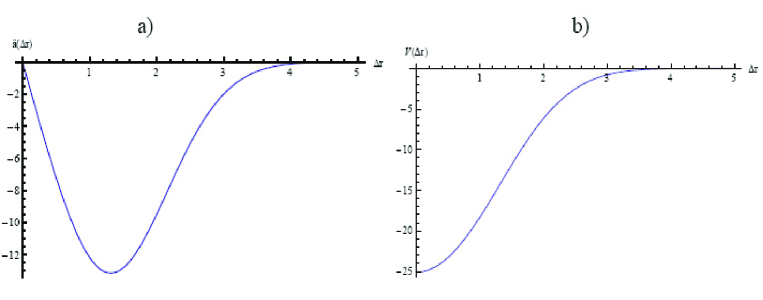
Figure 3: Graphics of the nonlinear acceleration $\ddot{a}(\Delta r)$ (IV) and potential $V(\Delta r)$ (19) between the centers of weight in cases of Gaussian pulses (20) for normalized constant $2\pi^{2}C_{1}A_{0}^{4}=1$.

On Fig. 3 the graphics of the nonlinear acceleration $\ddot{a}(\Delta r)$ (IV) and potential $V(\Delta r)$ (19) between the centers of weight in the cases of Gaussian pulses (20) for normalized constant $2\pi^{2}C_{1}A_{0}^{4}=1$ are presented. The same quantities for Lorentz pulses (21) are plotted on Fig. 4. The formulae of the exact solutions of the convolution integral (IV) and the potentials (19) for the both cases are

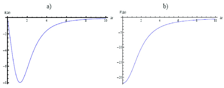
Figure 4: Graphics of the nonlinear acceleration $\ddot{a}(\Delta r)$ (IV) and potential $V(\Delta r)$ (19) between the centers of weight in cases of Lorentz pulses (21). The potential of Lorentz pulses is approximately twice wider than the potential of Gaussian ones.

$$\left\langle\ddot{a_{i}}^{Gaus}(\Delta r)\right\rangle=-2\sqrt{2\pi}\Delta r\left(3+\Delta r^{2}\right)\exp\left(-\Delta r/2\right);\,\,V^{Gaus}\left(\Delta r\right)=2\sqrt{2\pi}\left(5+\Delta r^{2}\right)\exp\left(-\Delta r/2\right).$$ (22)

$$\left\langle\ddot{a_{i}}^{Lorentz}(\Delta r)\right\rangle=-\frac{32\pi\Delta r\left(24+22\Delta r^{2}+\Delta r^{4}\right)}{\left(4+\Delta r^{2}\right)^{4}};\,\,V^{Lorentz}\left(\Delta r\right)=\frac{16\pi\Delta r\left(28+15\Delta r^{2}+\Delta r^{4}\right)}{\left(4+\Delta r^{2}\right)^{3}}).$$ (23)

It is important to be pointed that the potential of Lorentz pulses is approximately twice wider than the potential of Gaussian pulses. As a result, the Lorentz type filaments can interact at twice longer distance than the standard Gaussian type filaments. In the general case, the acceleration and the potential are not stationary and as it can be seen from the expressions (IV) and (19) depend in addition on the time. That is why the spatial forms and the spectrums of the pulses at short distances are modulated significantly. The numerical experiments demonstrate, that if the pulses are separated along $x$ direction, the forms and the $k_{x}$ spectrums of the both pulses become asymmetric.

V Conclusions

We have developed a vector model to describe the processes of reduction of number of the filaments as well as the observation of mergers and Rogue events during multi-filament propagation. It is known, that in air $P=P_{cr}$ corresponds to intensity of the laser field of the order of $I\sim 10^{12}$ $W/cm^{2}$. The main role at these intensities play the nonlinear $\chi^{(3)}$ effects. The results from the numerical analysis give confidence for claiming, that the investigated above processes are result of nonlinear interactions due to FPPM and CPM mechanisms. Finally, by using the method of moments, the merging between spherically-symmetric, circular polarized filaments is presented as potential interaction.

VI Acknowledgements

This work was supported in part by Bulgarian Science Fund under grant DFNI–I-02/9.

VII List of Figure Captions

Fig.1 (1a) Energy exchange between two collinear filaments $\vec{A}_{1}$ and $\vec{A}_{2}$ with power slightly above the critical $P_{cr}$ ($\gamma=1.5$). The pulses are separated initially at distance $2a=3.4$ and the evolution is governed by the system of equations (II). In the initial conditions (III) the phase difference $\varphi=\pi/4$ correspond to maximal energy exchange. Due to degenerated FPPM process one of the filaments is amplified while the other filament enters in linear mode and vanishes. (1b) Fusion between the same pulses when they are with equal initial phases, i. e. $\Delta\varphi=0$. The similar picture is seen when the FPPM terms are excluded from the equations (II) and only interaction due to CPM is investigated. With $z_{diff}$ is denoted the diffraction length $z_{diff}=k_{0}r_{0}^{2}$.

Fig.2 Interaction between three collinear filaments $\vec{A}_{1}$, $\vec{A}_{2}$ and $\vec{A}_{3}$ governed by the system of equations (II). Two of the pulses are with equal initial phases, while the third admits phase difference $\Delta\varphi=\pi/4$ in respect to others. Fusing between the pulses with equal phases is seen, while the third one exchanges energy by FPPM process.

Fig. 3 Graphics of the nonlinear acceleration $\ddot{a}(\Delta r)$ (IV) and potential $V(\Delta r)$ (19) between the centers of weight in cases of Gaussian pulses (20) for normalized constant $2\pi^{2}C_{1}A_{0}^{4}=1$.

Fig. 4 Graphics of the nonlinear acceleration $\ddot{a}(\Delta r)$ (IV) and potential $V(\Delta r)$ (19) between the centers of weight in cases of Lorentz pulses (21). The potential of Lorentz pulses is approximately twice wider than the potential of Gaussian ones.

References

- (1) S. Tzortzakis, L. Bergé, A. Couairon, M. Franco, B. Prade, A. Mysyrowicz, A., ”Break-up and fusion of self-guided femtosecond light pulses in air.” Phys. Rev. Lett. 86, pp. 5470–5473 (2001).
- (2) O. G. Kosareva, N. A. Panov, N. Aközbek, V. P. Kandidov, Q. Luo, S. A. Hosseini, W. Liu, J.-F. Gravel, G. Roy, S. L. Chin, ”Controlling a bunch of multiple filaments by means of a beam diameter.” Appl. Phys. B 82 (1), pp. 111–122 (2006).
- (3) Bonggu Shim et al., ”Controlled interactions of femtosecond light filaments in air”, Phys. Rev. A 81, 061803 (R) (2010).
- (4) S. V. Chekalin and V. P. Kandidov, ”From self- focusing light beams to femtosecond laser pulse filamentation”, Uspekhi Fizicheskikh Nauk, 183 , pp. 133 - 152 (2013).
- (5) S. Birkholz, E. T. J. Nibbering, C. Breé, S. Skupin, A. Demircan, G. Genty, and G. Steinmeyer, ”Spatiotemporal Rogue Events in Optical Multiple Filamentation”, Phys. Rev. Lett., 111, 243903 (2013).
- (6) J. Wahlstrand, N. Jhajj, E. W. Rosenthal, R. Birnbaum, S. Zahedpour, and H. M. Milchberg, ”Long-lived High Power Optical Waveguides in Air,” in Research in Optical Sciences , OSA Technical Digest (online) (Optical Society of America, 2014), paper HTh2B.4.
- (7) L. Bergé et al., ”Multiple Filamentation of Terawatt Laser Pulses in Air”, Phys. Rev. Lett. 92, 225002 (2004).
- (8) R. W. Boyd, Nonlinear Optics (Academic Press, San Diego, 1992), 2nd ed.
- (9) C. R. Menyuk, ”Stability of solitons in birefringent optical fibers. I: Equal propagation amplitudes,” Opt. Lett., 12, pp. 614–616 (1987);
- (10) C. R. Menyuk, ”Stability of solitons in birefringent optical fibers. II. Arbitrary amplitudes,” J. Opt. Soc. Am. B, 5, pp. 392–402 (1988).
- (11) V. V. Afanasiev, L. M. Kovachev and V. N. Serkin, ”Interaction of pulses on different frequencies”, Letters in JTP, 16, pp. 10–14 (1990).
- (12) L. M. Kovachev, ”Influence of cross-phase modulation and four-photon parametric mixing on the relative motion of optical pulses”, Optical and Quantum Electronics,23, pp. 1091-1102 (1991).
- (13) M. Kolesik, J. V. Moloney, ”Perturbative and non-perturbative aspects of optical filamentation in bulk dielectric media”, Optics Express, 16, 2971(2008);
- (14) M. Kolesik, E. M. Wright, A. Becker, J. V. Moloney, ”Simulation of third-harmonic and supercontinuum generation for femtosecond pulses in air” Appl. Phys. B, 85, pp. 531-538 (2006).
- (15) L. Kovachev and K. Kovachev, 2011, ”Linear and nonlinear femtosecond optics in isotropic media. Ionization-free filamentataion”, Laser Systems for Applications, Part 3, Chapter 11, InTech.
- (16) O. Kosareva et al., ”Polarization rotation due to femtosecond filamentation in an atomic gas”, Opt. Lett., 35, pp. 2904-2906 (2010).
- (17) A. H. Sheinfux, E. Schleifer, J. Papeer, G. Gibich, B. Ilan, and A. Zigler, Applied Physics Letters, ”Measuring the stability of polarization orientation in high intensity laser filaments in air”, 101, 201105 (2012).
- (18) M. Durand et al., ”Kilometer range filamentation”, Optics Express, 21, 26836 (2013).
- (19) Daniela A. Georgieva and Lubomir M. Kovachev, ”Energy transfer between two filaments and degenerate four-photon parametric processes”, Laser Physics 25, 035402 (2015).