A second order expansion of the separatrix map for trigonometric perturbations of a priori unstable systems

Abstract

In this paper we study a so-called separatrix map introduced by Zaslavskii-Filonenko [ZF68] and studied by Treschev and Piftankin [Tre98, Tre02, Pif06, PT07]. We derive a second order expansion of this map for trigonometric perturbations. In [CK15, GK15], and [KZZ15], applying the results of the present paper, we describe a class of nearly integrable deterministic systems with stochastic diffusive behavior.

1 Introduction

The main goal of this paper is to derive a second order expansion of a so-called separatrix map for a class of nearly integrable systems. In nearly integrable Hamiltonian systems with one and a half degree of freedom this map was introduced by Zaslavskii and Filonenko in [ZF68]. Shilnikov [Šil65], using a very similar geometric idea, studied it in a neighborhood of homoclinic orbits without restriction to Hamiltonian structure or closeness to integrability. Treschev and Piftankin estimated the error terms in the traditional version of the separatrix map and studied the multidimensional situation [Tre98, Tre02, Pif06].

It is becoming clear that the separatrix map is a powerful tool to analyze the dynamics in a neighbourhood of homoclinic orbits to a normally hyperbolic invariant manifold and instabilites of Hamiltonian systems (see the survey [PT07] and the papers by Treschev [Tre04, Tre12]). For this reason in [KZZ15], using results of this paper, we perform an indepth analysis of the phenomenon of global instabilities in nearly integrable Hamiltonian systems. Usually this phenomenon, discovered by Arnold [Arn64], is called Arnold diffusion.

The purpose of this paper is to have detailed studies of the multidimensional separatrix map, proposed in [Tre02], and to compute higher order expansion of this map with smaller remainder terms.

The main motivation for this work is to study certain stochastic diffusive behavior for nearly integrable deterministic systems. Such stochastic behavior was conjectured by Chirikov [Chi79] in the 1970s.

Recall a basic fact from probability theory, which is a non-homogenenous version of Donsker’s theorem (see e.g. [Eth05]). Let $\eta\in\mathbb{R}$, $\sigma(\eta)>0$ and $b(\eta)$ be two smooth functions of one variable. Fix $\delta>0,\ \eta_{0}\in\mathbb{R}$ and consider a sequence

$$\eta_{n+1}=\eta_{n}+\sigma(\eta_{n})\delta\,\omega_{n}+b(\eta_{n})\delta^{2},$$

where $\omega_{n}$’s are independent random variables taking values $1$ or $-1$ with equal probabilities. Then for each $s>0$ and $n_{\delta}=[s\delta^{-2}]$ as $\delta\to 0$ the distribution of $\eta_{n_{\delta}}$ converges weakly to the distribution of the Ito diffusion process starting at $\eta_{0}$ with the drift $b(\eta)$ and the variance $\sigma^{2}(\eta)$.

In the framework that we study in this paper, $\eta$ is an action variable of some Hamiltonian system. To study long time evolution of $\eta_{t}$ we consider a separatrix map and study a discrete version $\eta_{t_{n}},\ n>1$. Then the variance $\sigma(\eta)$ of the discrete version is given by an associated Melnikov function and was computed by Zaslavski (see (8) for a more precise claim). However, to analyze $\eta_{t}$ as a diffusion process we also need to compute the drift function $b(\eta)$. This is the main purpose of our paper.

In Appendix A we apply our analysis to the so-called generalized Arnold example and compute analogs of the drift $b(\eta)$ and the variance $\sigma(\eta)$. In [KZZ15] we combine these results with results from [CK15] (see also [GK15]) and construct a class of probability measures for a class of trigonometric perturbations of the generalized Arnold example. It turns out that the distributions of a certain action component under the associated Hamiltonian flow with respect to these measures weakly converge to a stochastic diffusion process on the line.

More precisely, in [KZZ15] for an open class of trigonometric perturbations for a time one map of a generalized Arnold example, which is a $4$-dimensional symplectic map $\mathcal{F}$, we construct a normally hyperbolic invariant lamination $\Lambda$. Leaves of this lamination are diffeomorphic to $2$-dimension cylinders $\mathbb{A}=\mathbb{T}\times\mathbb{R}$. We find a coordinate change such that the restriction of $F=\mathcal{F}|_{\Lambda}$ to this lamination is a skew-product of the form

$$F:\mathbb{A}\times\{0,1\}^{\mathbb{Z}},\qquad F(x,\omega)=(f_{\omega}(x),\sigma\omega),$$

where $\omega\in\{0,1\}^{\mathbb{Z}}$, $\sigma$ is the shift, and $f_{\omega}(x)$ is an exact area-preserving map of the $2$-dimensional cylinder $\mathbb{A}$. Loosely speaking, using the results of the present paper, we obtain a second order expansion of $f_{\omega}$’s in the perturbation parameter.

In [CK15] and [GK15] we analyze a class of skew products, which includes the aforementioned system $F(x,\omega)$, and prove weak convergence to a stochastic diffusion process on the line.

We emphasize that the previously known results on Arnold diffusion for the generalized Arnold example or, more generally, for a priori chaotic systems, or a priori unstable systems, or a priori stable systems, establish the existence of “special diffusing” orbits (see [Ber08, BKZ11, BT99, BK05, CY04, CY09, CZ13, Che13, DdlLS00, DdlLS06, DH09, DdlLS13, FGKP11, GT08, GdlL06, GK14, Kal03, KMV04, KL08a, KL08b, KS12, KZ12, KLS14, MS02, Mat91a, Mat91b, Mat93, Mat96, Mat03, Mat08, Moe96, Pif06, Tre04, Tre12]). In [KZZ15], [CK15], and [GK15], using the analysis of the present paper, we study deterministic evolution of a class of probability measures under the deperministic Hamiltonian flow and obtain that the distributions of a certain action component weakly converge to a stochastic diffusion process.

1.1 The separatrix map for the Arnold example

Since the definition and formulas of the separatrix map are rather involved, we start by considering a simple case: the generalized Arnold example. Later, in Section 1.2, we consider more general models. In this section we consider Hamiltonians of the form $H_{0}+\varepsilon H_{1}$ with

$$\begin{split}H_{0}(I,p,q)\ \ \ \ &=\ \dfrac{I^{2}}{2}+\dfrac{p^{2}}{2}+(\cos q-1),\\ H_{1}(I,\varphi,p,q,t)&=\ P(I,p,e^{iq},e^{i\varphi},e^{it}),\end{split}$$ (1)

where the unperturbed $H_{0}$ defines the product of the rotor and the pendulum and $P(I,p,e^{iq},e^{i\varphi},e^{it})$ is a real valued trigonometric polynomial in $\varphi$ and $t$. For the classical Arnold example $P=(1-\cos q)(\cos\varphi+\cos t)$.

In this section, we describe and provide “simple” formulas for the separatrix map for such models. The rigorous definition is provided in Section 2 and more accurate formulas for model (1) are derived in Appendix A.

The Hamiltonian of the pendulum $\frac{p^{2}}{2}+(\cos q-1)$ has a saddle at $(p,q)=(0,0)$ whose stable and unstable invariant manifolds coincide forming a figure eight (see left picture in Figure 1). In the full phase space, the saddle corresponds to the normally hyperbolic invariant manifold $(p,q)=(0,0)$, $I\in[I_{-},I_{+}]$, $\varphi\in\mathbb{T}$. The union of the figure eights for every value of $I\in[I_{-},I_{+}]$ form the stable and unstable manifolds of the normally hyperbolic cylinder. Consider a neighborhood of such set. It can be defined by

$$\left|\frac{p^{2}}{2}+(\cos q-1)\right|<c,\quad I\in[I_{-},I_{+}],\varphi\in\mathbb{T}$$

for some small $c>0$.

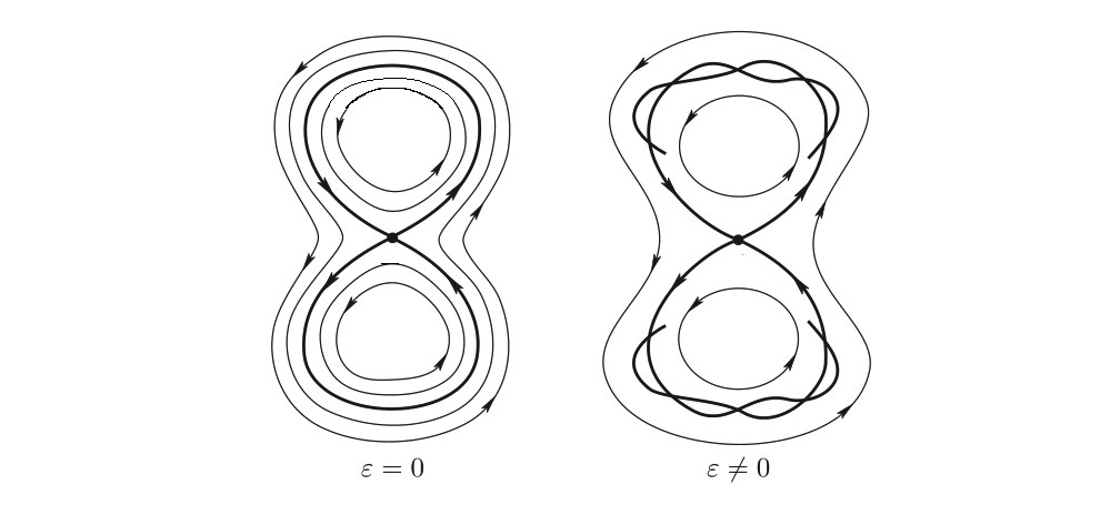
Figure 1: The figure $8$.

When one adds the perturbation $H_{1}$, typically, the invariant manifolds of the cylinder split. The goal of the separatrix map is to understand the dynamics in the neighborhood of the perturbed invariant manifolds, which now intersect transversally.

Now we describe the separatrix map. A more rigorous definition of the separatrix map is done in Section 2. Consider the time one map $T_{\varepsilon}$ associated to the flow of the Hamiltonian $H_{\varepsilon}$. We define two fundamental domains, as shown in Figure 2, as domains such that the image of any point in them under $T_{\varepsilon}$ does not belong to them and some iterate of any point near an unstable manifold intersects one of these domains. For any point in the fundamental domains one can keep iterating $T_{\varepsilon}$. If some iterate of such point enters again into one of the fundamental domains, we call this point the image of the initial point by the separatrix map. Note that some points may not have any of the further iterates in the fundamental domains, e.g. those belonging to stable invariant manifolds. Then, for these points, we say that the separatrix map is not defined. Sometimes, a map of this kind is also called an induced map or a return map.

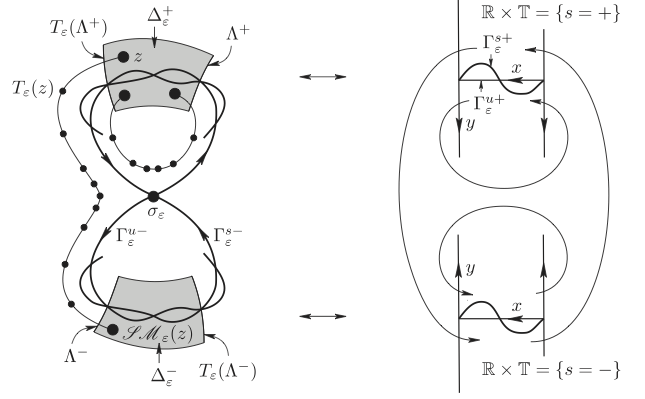
Figure 2: The fundamental domain

To give formulas for the separatrix map, we consider the Fourier expansion of the Hamiltonian $H_{1}(I,\varphi,0,0,t)$,

$$H_{1}(I,\varphi,0,0,t)=\sum_{|k|\leq N}H_{1}^{k}(I)e^{2\pi ik\cdot(\varphi,t)},$$

where $N>0$ is the degree of the trigonometric polynomial.

Let $\psi:\mathbb{R}\longrightarrow[0,1]$ be a $\mathcal{C}^{\infty}$ function such that $\psi(r)=0$ for any $|r|\geq 1$ and $\psi(r)=1$ for any $|r|\leq 1/2$. We define

$$\begin{split}\overline{\bf H}_{1}(I,\varphi,t)&=\sum_{|k|\leq N}\psi\left(\frac{k\cdot(I,1)}{\beta}\right)H_{1}^{k}(I)e^{2\pi ik\cdot(\varphi,t)}\\ {\bf H}_{1}(I,\varphi)&=\overline{\bf H}_{1}(I,\varphi,0),\end{split}$$

for some fixed $\beta>0$ independent of $\varepsilon$ small enough so that for every $I\in[I_{-},I_{+}]$ only one harmonic does not vanish (we do not have overlapping of resonant zones).

We consider a certain system of coordinates $(\eta,\xi,h,\tau,\sigma)$ in the fundamental domain (it is explained more precisely in Theorem 2.1). The last variable $\sigma\in\{-,+\}$ denotes the two connected components of the fundamental domain. We define the function

$$w_{0}(\eta^{*},h^{*},\xi^{*})=h^{*}-\frac{(\eta^{*})^{2}}{2}-\varepsilon{\bf H}_{1}(\eta^{*},\xi^{*}).$$

Then, in such coordinates, the separatrix map is defined for points such that $|w_{0}|\sim\varepsilon$ and has the following (implicit) form

$$\eta^{*}= \,\eta +\varepsilon\partial_{\xi}\Theta^{\sigma}(\eta,\xi,\tau)+\varepsilon B^{\eta,\sigma}(\eta,\xi,w_{0},\tau)+\mathcal{O}(\varepsilon^{5/3})$$

$$\xi^{*}= \,\xi +\qquad\qquad\qquad\qquad\eta\log\left|\kappa^{\sigma}w_{0}\right|+\mathcal{O}(\varepsilon\log\varepsilon)$$

$$h^{*}= \,h +\varepsilon\partial_{\tau}\Theta^{\sigma}(\eta,\xi,\tau)+\mathcal{O}(\varepsilon^{5/3})$$

$$\tau^{*}= \,\tau +\qquad\qquad\qquad\qquad\log\left|\kappa^{\sigma}w_{0}\right|+\mathcal{O}(\varepsilon\log\varepsilon)$$

$$\sigma^{*}= \,\sigma\ \mathrm{sgn}\ w_{0}$$

where $\kappa^{\sigma}>0$ are certain constants (see Section 2.1 and Appendix A),

$$B^{\eta,\sigma}(\eta,\xi,w_{0},\tau)=\frac{1}{\eta}\left({\bf\bar{H}}_{1}(\eta,\xi)-{\bf\bar{H}}_{1}(\eta,\xi+\eta\log\left|\kappa^{\sigma}w_{0}\right|)\right)$$

and $\Theta^{\sigma}$ are the Melnikov potentials, which are defined as

$$\Theta^{\sigma}(\eta,\xi,\tau)=\int_{-\infty}^{+\infty}\left(H_{1}\left(\Gamma^{\sigma}(\eta,\xi,\tau+t),t-\tau\right)-H_{1}\left(\eta,\varphi+\eta t,0,0,t-\tau\right)\right)\,dt,$$

where $\Gamma^{\sigma}$ are the time parameterization of the pendulum separatrices, that is

$$\Gamma^{\sigma}(\eta,\xi,\tau)=\left(\eta,\xi+\eta\tau,4\arctan(e^{\sigma\tau}),\frac{2\sigma}{\cosh\tau}\right).$$

Now we consider a more general set up, proposed by Treschev.

1.2 The set up

Consider a Hamiltonian system

$$H_{\varepsilon}(I,\varphi,p,q,t)=H_{0}(I,p,q)+\varepsilon H_{1}(I,\varphi,p,q,t),$$ (2)

where $I\in\mathbb{R}^{n}$ are actions, $\varphi\in\mathbb{T}^{n}$ are angles and $(p,q)$ belong to an open domain $D\subset\mathbb{R}^{2}$. Even if not written explicitly, the Hamiltonian $H_{1}$ may depend on the parameter $\varepsilon$. Fix a bounded open set $\mathcal{D}\subset\mathbb{R}^{n}$.

We assume that for every fixed $I\in\mathcal{D}$, the Hamiltonian $H_{0}(I,p,q)$ has a saddle at $(p,q)=(0,0)$ with two separatrix loops (see Fig. 1). In [Tre02] it is assumed the following hypotheses.

• The function $H$ is $\mathcal{C}^{5}$-smooth in all arguments while $H_{0}$ is real-analytic in $p,q$, and $\mathcal{C}^{5}$-smooth in $I$.

We consider the alternative assumption.

• The function $H_{0}$ is $\mathcal{C}^{r}$ and $H$ is $\mathcal{C}^{s}$-smooth in all arguments for $s\geq 6$ and $r\geq 8s+2$.

That is, we admit lower regularity on $H_{0}$. On $H_{1}$ we assume one degree more of regularity than in [Tre02]. It is needed to have better estimates of the separatrix map.

• For all points $I^{0}\in\mathcal{D}$, the function $H(I^{0},p,q)$ has a non-degenerate saddle point at $(p,q)=(p^{0},q^{0})$ smoothly depending on $I$. For all $I^{0}\in\mathcal{D}$, $(p^{0},q^{0})$ belongs to a connected component of the set

  $$\{(p,q):\,H_{0}(I^{0},p,q)=H_{0}(I^{0},p^{0},q^{0})\}.$$

  Moreover, $(p^{0},q^{0})$ is the unique critical point of $H_{0}(I^{0},p,q)$ in this component.

Remark 1.1.

Using Prop.1, [Tre02], if one assumes that the saddle is at a certain point $(p,q)=(p^{0},q^{0})$ which depends smoothly on $I$, then, one can perform a symplectic change of coordinates so that the critical point is at $(p,q)=(0,0)$ for all $I\in\mathcal{D}$. After such a coordinate change $\mathcal{C}^{r}$ in H1 is replaced by $\mathcal{C}^{r-2}$.

We denote the loops of the “eight” given by Hypothesis H2 by $\gamma^{\pm}(I^{0})$. These loops have the natural orientation generated by the flow of the system (see Fig. 1). We can define an orientation in $D$ by the coordinate system $(p,q)$.

• For all $I^{0}\in\mathcal{D}$, the natural orientation of $\gamma^{\pm}(I^{0})$ coincides with the orientation of the domain, i. e. the motion of the separatrices is counterclockwise.

In [Tre02], Treschev defines the separatrix map for Hamiltonians satisfying these hypotheses and obtains a formula for this map with certain remainder terms. The goal of this paper is to refine Treschev formulas in several aspects.

Note that the formulas for the separatrix map present certain differences in what are called a non-resonant and a resonant regime (see below). Treschev provides global formulas for the separatrix map. Here we separate the two regimes and give more precise formulas. The refinements we do are the following.

• For the non-resonant regime we compute the separatrix map up to 2nd order in $\varepsilon$.

• For the resonant regime we give formulas in slow-fast variables and we improve the size of the remainders.

We obtain formulas for general Hamiltonians, but also pay attention to the particular case of the generalized Arnold example (1). The results for such model are presented in Appendix A.

Acknowledgement The authors thank Dmitry Treschev for helpful discussions and remarks on the preliminary version of the paper. The authors also acknowledge many useful discussion with Ke Zhang. The first author is partially supported by the Spanish MINECO-FEDER Grant MTM2012-31714 and the Catalan Grant 2014SGR504. The second author acknowledges NSF for partial support grant DMS-5237860.

2 The separatrix map: Treschev’s results

We devote this section to define the separatrix map and state the results obtained in [Tre02].

We want to define a separatrix map for points whose $(p,q)$-components are “near” the unperturbed separatrices (see the shaded region on Fig. 3 below). For the unperturbed system there is a normally hyperbolic invariant cylinder $\Lambda=\{p=q=0\}$ and for each $I^{0}\in\mathcal{D}$ we have invariant tori

$$\Lambda(I^{0}):=\{I=I^{0},p=q=0\}=\Lambda\cap\{I=I^{0}\}.$$

These tori are (partially) hyperbolic, i.e there are expanding and contracting directions dominating the other ones. There exist two asymptotic manifolds,

$$\begin{split}\widehat{\Gamma}^{\pm}(I^{0})&\subset\{(I^{0},\varphi,p,q,t):\ \varphi,t\in\mathbb{T},\ H_{0}(I^{0},p,q)=0\}\\ \widehat{\Gamma}^{\pm}(I^{0})&=\{I^{0}\}\times\mathbb{T}\times\gamma^{\pm}(I_{0})\times\mathbb{T},\end{split}$$

where $\gamma^{\pm}(I_{0})$ are the two separatrices in the $(p,q)$ plane. The manifolds $\widehat{\Gamma}^{\pm}(I^{0})$ consist of unperturbed solutions that approach $\Lambda(I^{0})$.

Assume that $\mathcal{D}$ is an open connected domain with compact closure $\overline{\mathcal{D}}$. In what follows, we consider the dynamics of the non-perturbed system in a neighbourhood of the unstable and stable manifolds of the cylinder $\Lambda$:

$$\widehat{\Gamma}=\cup_{I\in\overline{\mathcal{D}}}\left(\widehat{\Gamma}^{+}(I)\cup\widehat{\Gamma}^{-}(I)\right).$$

This neighbourhood contains the most interesting part of the perturbed dynamics. It is convenient to pass to the time one map $T_{\varepsilon}$: for any point $(I,\varphi,p,q)$

$$T_{\varepsilon}:(I,\varphi,p,q)\longrightarrow(I(1),\varphi(1),p(1),q(1)),$$

where $(I(t),\varphi(t),p(t),q(t))$ is the solution of the Hamiltonian system given by $H_{\varepsilon}$ with initial conditions $(I(0),\varphi(0),p(0),q(0))=(I,\varphi,p,q)$. The map $T_{0}$ has $1$-dimensional hyperbolic tori $L(I)=\pi(\Lambda(I))$, where the map $\pi:(I,\varphi,p,q,t)\to(I,\varphi,p,q)$ is the natural projection. Let $\Sigma^{\pm}(I)=\pi(\widehat{\Gamma}^{\pm}(I))$ be the invariant manifolds (see Fig. 3). We define the separatrix map $\mathcal{SM}_{\varepsilon}$ corresponding to $T_{\varepsilon}$ in a neighbourhood of the set

$$\Sigma=\cup_{I\in\overline{\mathcal{D}}}\left(\Sigma^{+}(I)\cup\Sigma^{-}(I)\right)=\pi(\widehat{\Gamma}).$$

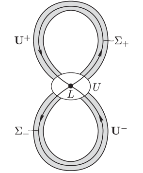
Figure 3: Neighbourhoods about the figure $8$.

Let $U$ be a small neighbourhood of the set $\cup_{I\in\overline{\mathcal{D}}}L(I)$ and let $\bf U$ be a neighbourhood of $\Sigma$ (see Figure 3, where $\Sigma$ is pictured in the case $n=0$). If $\bf U$ is sufficiently small, then ${\bf U}\setminus U$ consists of two connected components $\bf U^{+}$ and $\bf U^{-}$, and, thus, $\Sigma^{\pm}\subset\bf U^{\pm}\cup U$.

Consider a point $z\in\bf U^{+}\cup\bf U^{-}$. Let $k_{1}=k_{1}(z)$ be the minimal positive integer such that $T^{k_{1}}_{\varepsilon}(z)\not\in\bf U^{+}\cup\bf U^{-}$ and let $k_{2}=k_{2}(z)$ be the minimal positive integer such that $k_{2}>k_{1}$ and $T^{k_{2}}_{\varepsilon}(z)\in\bf U^{+}\cup\bf U^{-}$. The trajectory $T^{k}_{\varepsilon}(z)$ leaves $\bf U^{+}\cup\bf U^{-}$ at $k=k_{1}$, and it returns to $\bf U^{+}\cup\bf U^{-}$ at $k=k_{2}$. A point $z$ is said to be good if $k_{2}<+\infty$ and $T^{k_{1}}_{\varepsilon}(z),\dots,T^{k_{2}-1}_{\varepsilon}(z)\in U$. Setting

$${\bf U}_{\varepsilon}=\{z\in{\bf U^{+}}\cup{\bf U^{-}}:\ z\text{ is good}\}$$

we obtain maps

$$\mathcal{SM}_{\varepsilon}(\cdot,k_{2}(\cdot)+k):\ {\bf U}_{\varepsilon}\to\bf U^{+}\cup\bf U^{-},$$

$$\mathcal{SM}_{\varepsilon}(z,k_{2}(z)+k)=T^{k_{2}(z)+k}_{\varepsilon}(z).$$

Here $k\in\{0,1,\dots\}$ is a parameter, and it is assumed that

$$T^{k_{2}(z)+1}_{\varepsilon}(z),\dots,T^{k_{2}(z)+k}_{\varepsilon}(z)\in\bf U^{+}\cup\bf U^{-}.$$

In [PT07] it is set $t_{+}=k_{2}(z)+k$. Since neither $\bf U^{+}$ nor $\bf U^{-}$ serves as a fundamental domain, there is a considerable freedom for $k$. We would like to avoid this freedom. By analogy with the pendulum case (see Fig. 2) we let $\Lambda^{+}$ and $\Lambda^{-}$ be hyperplanes in $\mathbb{A}\times\mathbb{A}\times\mathbb{T}\ni(I,\varphi,p,q,t)$ whose projection onto the $(p,q)$-component are curves going from one of the connected components of the boundary of $|H_{0}|<c$ to another and transversal to the upper and lower separatrix loops. We denote by $\Delta^{\pm}$ the subdomain of $U_{c}$ between the curves $\Lambda^{\pm}$ and $T_{\varepsilon}(\Lambda^{\pm})$ (see Fig. 2). We choose such $k$ above that $T^{k_{2}(z)+k}_{\varepsilon}(z)\in\Delta^{+}\cup\Delta^{-}$.

To provide formulas for the separatrix map we need to set up some notation. We define

$$E(I)=H_{0}(I,0,0),\quad\nu(I)=\partial_{I}E(I):\mathcal{D}\longrightarrow\mathbb{R}^{n}.$$ (3)

The Hamiltonian $H_{1}(I,\varphi,0,0,t)$ has the Fourier expansion

$$H_{1}(I,\varphi,0,0,t)=\sum_{k\in\mathbb{Z}^{n+1}}H_{1}^{k}(I)e^{2\pi ik\cdot(\varphi,t)}.$$

Let $\psi:\mathbb{R}\longrightarrow[0,1]$ be a $\mathcal{C}^{\infty}$ function such that $\psi(r)=0$ for any $|r|\geq 1$ and $\psi(r)=1$ for any $|r|\leq 1/2$. We define

$$\begin{split}\overline{\bf H}_{1}(I,\varphi,t)&=\sum_{k\in\mathbb{Z}^{n+1}}\psi\left(\frac{k\cdot(\nu(I),1)}{\beta}\right)H_{1}^{k}(I)e^{2\pi ik\cdot(\varphi,t)}\\ {\bf H}_{1}(I,\varphi)&=\overline{\bf H}_{1}(I,\varphi,0),\end{split}$$ (4)

for some constant $\beta>0$.

To obtain quantitative estimates, we follow [Tre02] and use skew norms, defined as follows. Let $K\subset\mathbb{R}^{m}$ be a compact set and $j\in\mathbb{N}$. Then, for functions $f\in\mathcal{C}^{j}(\overline{\mathcal{D}}\times K)$ we define

$$\|f(I,z)\|_{j}^{(b)}=\max_{0\leq l^{\prime}+l^{\prime\prime}\leq j}b^{l^{\prime}}\left|\frac{\partial^{l^{\prime}+l^{\prime\prime}}f}{\partial^{l^{\prime}_{1}}{I_{1}}\cdots\partial^{l^{\prime}_{n}}{I_{n}}\partial^{l^{\prime\prime}_{1}}{z_{1}}\cdots\partial^{l^{\prime\prime}_{m}}{z_{m}}}\right|,$$

where $l^{\prime\prime}=l_{1}^{\prime\prime}+\dots+l_{m}^{\prime\prime}$. It is assumed that $f$ can take values in $\mathbb{R}^{s}$, where $s$ is an arbitrary positive integer. The norms $\|\cdot\|^{(b)}_{r}$ are anisotropic, and the variables $r$ play a special role in these norms because the additional factor $b$ corresponds to the derivatives with respect to $r$. Obviously, $\|\cdot\|^{(1)}_{r}$ is the usual $\mathcal{C}^{r}$-norm. This norm is similar to the skew-symmetric norm introduced in [KZ12], Section 7.2.

For a function $f\in\mathcal{C}^{r}(\bar{\mathcal{D}}\times\bf K)$ and $g\in\mathcal{C}^{0}(\bar{\mathcal{D}}\times\bf K)$ we say that

$$f=\mathcal{O}^{(b)}_{0}(g)\ \textup{ if }\ \|f\|_{r}^{(b)}\leq C\,|g|^{k},$$

where $C$ does not depend on $b$. For brevity we write

$$\|\cdot\|_{r}^{*}=\|\cdot\|_{r}^{(\varepsilon^{\delta})},\ \ \ \mathcal{O}^{(b)}=\mathcal{O}^{(b)}_{1},\ \ \ \mathcal{O}^{*}_{k}=\mathcal{O}^{(\varepsilon^{\delta})}_{k}.$$ (5)

First, we state the result obtained in [Tre02]. He sets $b=\varepsilon^{1/4}$.

Theorem 2.1 ([Tre02]).

Let conditions [H1-H3] hold. Then, there exist $\mathcal{C}^{2}$ smooth functions

$$\lambda,\kappa^{\pm},\mu^{\pm}:\overline{\mathcal{D}}\rightarrow\mathbb{R},\qquad\Theta^{\pm}:\overline{\mathcal{D}}\times\mathbb{T}^{n+1}\rightarrow\mathbb{R},$$

and canonical coordinates $(\eta,\xi,h,\tau)$ such that the following conditions hold.

• $\omega=d\eta\wedge d\xi+dh\wedge d\tau$.

• $\eta=I+\mathcal{O}^{(\varepsilon^{1/4})}(\varepsilon^{3/4},H_{0}-E(I)),\ \xi+\nu(\eta)\tau=\varphi+f,\ h=H_{0}+\mathcal{O}^{(\varepsilon^{1/4})}(\varepsilon^{3/4},H_{0}-E(I)),$ where $f$ denotes a function depending only on $(I,p,q,\varepsilon)$ satisfying $f(I,0,0,0)=0$.

• Define

  $$w_{0}^{\sigma}=h^{*}-E(\eta^{*})-\varepsilon{\bf H}_{1}(\eta^{*},\xi+\nu(\eta^{*})\tau+\mu^{\sigma}(\eta^{*})).$$ (6)

  For any $\sigma=\{+,-\}$ and $(\eta^{*},\xi,h^{*},\tau)$ such that

  $$\begin{split}c^{-1}\varepsilon^{5/4}|\log\varepsilon|<|w_{0}^{\sigma}|\leq c\varepsilon^{7/8}\quad\\ |\tau|<c^{-1}\quad c<|w_{0}^{\sigma}|\,e^{\lambda(\eta^{*})\overline{t}}<c^{-1},\end{split}$$ (7)

  the separatrix map $(\eta^{*},\xi^{*},h^{*},\tau^{*})=\mathcal{SM}(\eta,\xi,h,\tau)$ is defined implicitly as follows

  $$\eta^{*}= \eta- \varepsilon\partial_{\xi}\Theta^{\sigma}(\eta^{*},\xi,\tau)\ -\frac{\partial_{\xi}w_{0}^{\sigma}}{\lambda}\log\left|\frac{\kappa^{\sigma}w_{0}^{\sigma}}{\lambda}\right|+{\bf O}_{2}$$ (8)

  $$\xi^{*}= \xi+\mu^{\sigma}+ \varepsilon\partial_{\eta^{*}}\Theta^{\sigma}(\eta^{*},\xi,\tau)+\frac{\partial_{\eta^{*}}w_{0}^{\sigma}}{\lambda}\log\left|\frac{\kappa^{\sigma}w_{0}^{\sigma}}{\lambda}\right|+{\bf O}_{1}$$

  $$h^{*}= h- \varepsilon\partial_{\tau}\Theta^{\sigma}(\eta^{*},\xi,\tau)\ -\frac{\partial_{\tau}w_{0}^{\sigma}}{\lambda}\log\left|\frac{\kappa^{\sigma}w_{0}^{\sigma}}{\lambda}\right|+{\bf O}_{2}$$

  $$\tau^{*}= \tau+\overline{t}+ \frac{\partial_{h^{*}}w_{0}^{\sigma}}{\lambda}\log\left|\frac{\kappa^{\sigma}w_{0}^{\sigma}}{\lambda}\right|+{\bf O}_{1}$$

  $$\sigma^{*}= \sigma\ \mathrm{sgn}w_{0}^{\sigma},$$

  where $\lambda$, $\kappa^{\pm}$ and $\mu^{\pm}$ are functions of $\eta^{*}$, $\overline{t}$ is an integer such that

  $$\left|\tau+\overline{t}+\frac{\partial_{h^{*}}w_{0}^{\sigma}}{\lambda}\log\left|\frac{\kappa^{\sigma}w_{0}^{\sigma}}{\lambda}\right|\right|<c^{-1}$$ (9)

  and ${\bf O}_{1}=\mathcal{O}^{(\varepsilon^{1/4})}(\varepsilon^{7/8})\log^{2}\varepsilon$, ${\bf O}_{2}=\mathcal{O}^{(\varepsilon^{1/4})}(\varepsilon^{5/4})\log^{2}\varepsilon$.

Remark 2.2.

Recall that the Hamiltonian $H_{\varepsilon}$ has a normally hyperbolic invariant cylinder $\Lambda_{\varepsilon}$ close to $\Lambda_{0}=\{p=q=0\}$. Dynamics of $H_{\varepsilon}$ restricted to $\Lambda_{\varepsilon}$ is often called inner dynamics. Dynamics of orbits belonging to the intersection of $W^{s}(\Lambda_{\varepsilon})$ and $W^{u}(\Lambda_{\varepsilon})$ is called outer dynamics and thoroughly studied in [DdlLS06, DdlLS08].

It is helpful to have Figure 2 in mind.

An heuristic explanation of the separatrix map is the following: every orbit starting in the fundamental region $\Delta$ and sufficiently close to the stable manifold $W^{s}(\Lambda_{\varepsilon})$ has three regimes:

— approaching the cylinder $\Lambda_{\varepsilon}$;

— evolution near $\Lambda_{\varepsilon}$

— departing away from $\Lambda_{\varepsilon}$ and reaching the fundamental domain.

In each of these three regimes we have:

— Straightening invariant manifolds trivialized the first regime.

— The Hamiltonians $w_{0}^{\sigma}$ approximate the evolution in the 2nd regime.

— The splitting potentials $\Theta^{\sigma}$ describe the third regime with an error.

It is reasonable to refer to the regime 2) as inner dynamics, since orbits near the cylinder $\Lambda_{\varepsilon}$ can be shadowed by orbits inside of the cylinder.

It is reasonable to call outer dynamics to the regime 1)+3). The outer dynamics to the leading order is well described by the splitting potentials $\Theta^{\sigma}$.

Look now at the formula (7). The separatrix map has contribution from the $w_{0}^{\sigma}$, which is the inner dynamics, and from $\Theta^{\sigma}$, which are the splitting potentials.

2.1 Formulas for auxuliary functions $\lambda,\kappa^{\pm},\mu^{\pm}$ and $\Theta^{\sigma}$

The functions $\lambda>0$, $\kappa^{\pm}>0$ and $\mu^{\pm}\in\mathbb{R}$ are defined by the unperturbed Hamiltonian $H_{0}$ as follows. Hypothesis H2 implies that both eigenvalues of the matrix

$$\Lambda(I)=\begin{pmatrix}-\partial_{pq}H_{0}(I,0,0)&-\partial_{qq}H_{0}(I,0,0)\\ \ \ \ \partial_{pp}H_{0}(I,0,0)\ &\partial_{pq}H_{0}(I,0,0)\end{pmatrix}$$ (10)

are real and the trace of this matrix is equal to 0 for all $I$. We denote by $\lambda(I)$ the positive eigenvalue of this matrix.

We denote by $\gamma^{\pm}(I,\cdot):\mathbb{R}\longrightarrow\mathbb{R}^{2}$ the time parameterization of the upper and lower separatrices of $H_{0}$ in the level of energy $H_{0}(I,p,q)=H_{0}(I,0,0)$. We denote by $a_{\pm}(I)$ the left eigenvectors of the matrix $\Lambda(I)$, that is, $a_{+}\Lambda=\lambda a_{+}$ and $a_{-}\Lambda=-\lambda a_{-}$, such that the $2\times 2$ matrix with $a_{\pm}$ as columns has determinant equal to one.

Then, we define

$$\mu^{\pm}(I) =\int_{-\infty}^{+\infty}(-\nu(I)+\partial_{I}H_{0}(I,\gamma^{\pm}(I,t)))\,dt$$ (11)

$$(\kappa^{\pm})^{-1}(I) =\lim_{t\longrightarrow+\infty}\left[\langle a_{+}(I),\gamma^{\pm}(I,-t)\rangle\langle a_{-}(I),\gamma^{\pm}(I,t)\rangle e^{2\lambda(I)t}\right].$$ (12)

To define the functions $\Theta^{\sigma}$, we have to introduce some notation. We define the differential operator

$$\partial=\nu(I)\partial_{\varphi}+\partial_{\tau}.$$ (13)

Fix $\beta>0$. The inverse operator $\partial^{-1}$ is defined on the “resonant” space

$$\mathrm{Res}=\left\{f:\overline{\mathcal{D}}\times\mathbb{T}^{n+1}:f^{k,k_{0}}=0\ \ \text{ if }\ \ |\langle k,\nu(I)\rangle+k_{0}|\leq\beta/2\right\},$$

where $f^{k,k_{0}}$ are the Fourier coefficients of $f$. Then, for $f\in\mathrm{Res}$, we have that $\partial^{-1}f$ is well defined and satisfies

$$\partial^{-1}f=\mathcal{O}^{*}(\beta^{-1}f).$$

As we have already mentioned, Treschev in [Tre02] chooses $\beta=\varepsilon^{1/4}$.

We define

$$\vartheta^{\sigma}(I,\varphi,\tau)=-\partial^{-1}\left[H_{1}(I,\varphi,0,0,\tau)-\overline{\bf H}_{1}(I,\varphi,\tau)\right].$$ (14)

where $\overline{\bf H}_{1}$ is the Hamiltonian defined in (4).

Any solution of the unperturbed system lying on $\widehat{\Gamma}^{\pm}(I)$ can be written as

$$(I,\varphi,p,q)(t)=\Gamma^{\sigma}(I,\varphi,\tau+t)$$

with

$$\Gamma^{\sigma}(I,\varphi,\tau)=(I,\varphi+\nu(I)\tau+\chi^{\pm}(I,\tau),\gamma^{\pm}(I,\tau))$$

where $\chi^{\pm}(I,\tau)$ are solutions of

$$\dot{\chi}^{\pm}(I,t)=-\nu(I)+\partial_{I}H_{0}(I,\gamma^{\pm}(I,t)),\qquad\lim_{t\longrightarrow-\infty}\chi^{\pm}(I,t)=0.$$

By the definition of $\mu^{\sigma}$ in (11),

$$\mu^{\pm}(I)=\lim_{t\longrightarrow+\infty}\chi^{\pm}(I,t).$$

We define

$$H_{\pm}^{\sigma}(I,\varphi,\tau,t) =$$

$$H_{1} (\Gamma^{\sigma}(I,\varphi,t),t-\tau)-H_{1}(I,\varphi+\nu t+\chi^{\sigma}(I,\pm\infty),0,0,t-\tau).$$

Note that $H_{\pm}^{\sigma}(I,\varphi,\tau,t)$ tend to zero exponentially as $t\longrightarrow\pm\infty$.

Then,

$$\begin{split}\Theta^{\sigma}(I,\varphi,\tau)=&\vartheta^{\sigma}(I,\varphi,-\tau)-\vartheta^{\sigma}(I,\varphi+\mu^{\sigma},-\tau)\\ &-\int_{-\infty}^{0}H^{\sigma}_{-}(I,\varphi,\tau,t)\,dt-\int^{+\infty}_{0}H_{+}^{\sigma}(I,\varphi,\tau,t)\,dt.\end{split}$$ (15)

In [Tre02] these functions are called splitting potentials. The integral term is the classical Melnikov potential (also often called the Poincaré function, see for instance [DG00]).

As we have explained the purpose of this paper is to refine the formulas given in Theorem 2.1.

3 The finite harmonics setting

To get more precise formulas for the separatrix map in the finite harmonics setting, we consider different regions where it is defined. These regions overlap each other.

First fix some notation. Take a function $f:\mathbb{T}^{n}\times\mathbb{R}^{n}\times\mathbb{R}^{2}\times\mathbb{T}\longrightarrow\mathbb{R}$ with Fourier series

$$f=\sum_{k\in\mathbb{Z}^{n+1}}\,f^{k}(I,p,q)e^{2\pi ik\cdot(\varphi,t)}.$$

Define $\mathcal{N}$ as

$$\mathcal{N}(f)=\{k\in\mathbb{Z}^{n+1}:f^{k}\neq 0\}$$

and

$$\mathcal{N}^{(2)}(f)=\{k\in\mathbb{Z}^{n+1}:k=k_{1}+k_{2},k_{1},k_{2}\in\mathcal{N}(f)\}.$$

Consider the non-resonant region, which stays away from the resonances created by the harmonics in $\mathcal{N}(H_{1})\cup\mathcal{N}^{(2)}(H_{1})$.

Define

$$\mathrm{NR}_{\beta}=\left\{I:\forall k\in\mathcal{N}(H_{1})\cup\mathcal{N}^{(2)}(H_{1}),\,\,|k\cdot(\nu(I),1)|\geq\beta\right\},$$ (16)

for a fixed parameter $\beta$. The complement of the non-resonant zone is build up by the different resonant zones associated to the harmonics in $\mathcal{N}(H_{1})\cup\mathcal{N}^{(2)}(H_{1})$. Fix $k\in\mathcal{N}(H_{1})\cup\mathcal{N}^{(2)}(H_{1})$, then we define the resonant zone

$$\mathrm{Res}^{k}_{\beta}=\left\{I:|k\cdot(\nu(I),1)|\leq\beta\right\}.$$ (17)

The parameter $\beta$ in both regions will be chosen differently, so that the different zones overlap.

We abuse notation and we redefine the norms in (5) as

$$\|\cdot\|_{r}^{*}=\|\cdot\|_{r}^{(\beta)},\ \ \ \mathcal{O}^{(b)}=\mathcal{O}^{(b)}_{1},\ \ \ \mathcal{O}^{*}_{k}=\mathcal{O}^{(\beta)}_{k}.$$

for fixed $\beta>0$. Now we can give formulas for the separatrix map in both regions.

3.1 The separatrix map in the non-resonant regime

The main result of this section is Theorem 3.1 which gives refined formulas for the separatrix map in the non-resonant zone (see (16)). To state it we need to define an auxiliary function $w$. This $w$ is a slight modification of the functions $w_{0}^{\sigma}$ given in (6).

Consider a function $g(\eta,r)$. It is obtained in Section 4.1 by applying Moser’s normal form to $H_{0}$. This function $g$ satisfies $g(\eta,r)=\lambda(\eta)r+\mathcal{O}(r^{2})$, where $\lambda$ is the positive eigenvalue of the matrix (10). Therefore, $g$ is invertible with respect to the second variable for small $r$. Somewhat abusing notation, call $g_{r}^{-1}$ the inverse of $g$ with respect to the second variable . Then, we define the function $w$ by

$$w(\eta^{*},h^{*})=g_{r}^{-1}(\eta^{*},h^{*}-E(\eta^{*})).$$ (18)

Note that in the nonresonant regime, $w$ does not depend on whether we are close to one of the unperturbed homoclinic loops or the other, as happened in Theorem 2.1.

Theorem 3.1.

Fix $\beta>0$ and $1\geq a>0$. Let conditions [H1^′,H2,H3] hold for some $s\geq 6$, $r\geq 8s+2$. Then for $\varepsilon$ sufficiently small there exist $c>0$ independent of $\varepsilon$ and a $\mathcal{C}^{s-4}$ canonical coordinates $(\eta,\xi,h,\tau)$ such that in the non-resonant zone $\mathrm{NR}_{\beta}$ the following conditions hold:

• the canonical form $\omega=d\eta\wedge d\xi+dh\wedge d\tau$;

• $\eta=I+\mathcal{O}^{*}_{1}(\varepsilon)+\mathcal{O}^{*}_{2}(H_{0}-E(I)),\,\xi+\nu(\eta)\tau=\varphi+f,\,h=H_{0}+\mathcal{O}^{*}_{1}(\varepsilon)+\mathcal{O}^{*}_{2}(H_{0}-E(I)),$ where $f$ denotes a function depending only on $(I,p,q,\varepsilon)$ and such that $f=\mathcal{O}(w+\varepsilon),\ f(I,0,0,0)=0$.

• In these coordinates $\mathcal{SM}_{\varepsilon}$ has the following form. For any $\sigma\in\{-,+\}$ and $(\eta^{*},h^{*})$ such that

  $$c^{-1}\varepsilon^{1+a}<|w(\eta^{*},h^{*})|<c\varepsilon,\qquad|\tau|<c^{-1},\qquad c<|w(\eta^{*},h^{*})|\,e^{\lambda(\eta^{*})\overline{t}}<c^{-1},$$

  the separatrix map $(\eta^{*},\xi^{*},h^{*},\tau^{*})=\mathcal{SM}_{\varepsilon}(\eta,\xi,h,\tau)$ is defined implicitly as follows

  $$\begin{split}\eta^{*}=&\ \eta-\ \ \varepsilon M_{1}^{\sigma,\eta}+\ \ \varepsilon^{2}M_{2}^{\sigma,\eta}+\ \ \mathcal{O}_{3}^{*}(\varepsilon)|\log\varepsilon|\\ \xi^{*}=&\ \xi+\ \partial_{1}\Phi^{\sigma}(\eta,w(\eta^{*},h^{*}))+\partial_{\eta}w(\eta^{*},h^{*})\left[\log|w(\eta^{*},h^{*})|+\partial_{2}\Phi^{\sigma}(\eta^{*},w(\eta^{*},h^{*}))\right]\\ &+\mathcal{O}_{1}^{*}(\varepsilon)\,|\log\varepsilon|\\ h^{*}=&\ h-\ \ \varepsilon M_{1}^{\sigma,h}+\ \ \varepsilon^{2}M_{2}^{\sigma,h}+\ \ \mathcal{O}_{3}^{*}(\varepsilon)\\ \tau^{*}=&\ \tau+\ \qquad\qquad\overline{t}\qquad\quad+\partial_{h}w(\eta^{*},h^{*})\left[\log|w(\eta^{*},h^{*})|+\partial_{2}\Phi^{\sigma}(\eta^{*},w(\eta^{*},h^{*}))\right]\\ &+\mathcal{O}_{1}^{*}(\varepsilon)\,|\log\varepsilon|,\end{split}$$

  where $w$ is the function defined in (18), $M^{*}_{i}$ and $\Phi^{\pm}$ are some $\mathcal{C}^{s-4}$ functions and $\bar{t}$ is an integer satisfying (9). The functions $M_{i}^{*}$ are evaluated at $(\eta^{*},\xi,h^{*},\tau)$.

This theorem is proven in Section 7.

Remark 3.2.

The change of coordinates in the above Theorem is $\varepsilon$-close (in the $\mathcal{C}^{2}$-norm) to the system of coordinates obtained in Theorem 2.1.

The function $M^{*}_{i}$ and $\Phi^{\pm}$ are defined in Lemmas 6.1 and 7.2 respectively,

The functions $\Phi^{\sigma}$ are the generalizations of the functions $\mu^{\sigma}$ and $\kappa^{\sigma}$. Indeed, they satisfy

$$\partial_{\eta}\Phi^{\sigma}(\eta,r)=\mu^{\sigma}(\eta)+\mathcal{O}^{*}_{2}(r)\ \ \text{ and }\ \ e^{\partial_{r}\Phi^{\sigma}(\eta,r)}=\kappa^{\sigma}(\eta)+\mathcal{O}^{*}_{2}(r).$$

Moreover, the functions $M_{i}^{\sigma,i}$ satisfy

$$M_{1}^{\sigma,\eta}=\partial_{\xi}\Theta^{\sigma}+\mathcal{O}^{*}_{2}(w),\qquad M_{1}^{\sigma,h}=\partial_{\tau}\Theta^{\sigma}+\mathcal{O}^{*}_{2}(w),$$

where $\Theta^{\sigma}$ is the splitting potential given in (15) (compare with the formulas in Theorem 2.1). These last formulas are obtained in Lemma 7.3.

Remark 3.3.

We compare this Theorem with Theorem 2.1 and the Remark afterward. Notice that the inner dynamics in non-resonant zones can be made integrable and essentially decoupled from the outer dynamics. This is reflected in the fact that the $\eta$ and the $h$-components have no contribution from $w$ as the inner dynamics is integrable.

The splitting potential contributions and the integrable contributions to rotation of the angular components are essentially the same.

Consider the following useful example:

$$H_{\varepsilon}(I,\varphi,p,q,t)=\frac{I^{2}}{2}+\frac{p^{2}}{2}+(\cos q-1)+\varepsilon H_{1}(I,\varphi,t).$$

Notice that the perturbation does not affect the pendulum. As the result the perturbed system is the product of the pendulum and a perturbed rotor. Notice that $\overline{\bf H}_{1}(I,\varphi,t)=H_{1}(I,\varphi,t)$ and it is non-vanishing. Moreover, the splitting potential $\Theta^{\sigma}$ vanishes. Since $w^{\sigma}_{0}$, defined in (6), measures the trasition time $\bar{t}$ of the separatrix map $\mathcal{SM}_{\varepsilon}$ (see (7)), it has to be independent of angles of the rotor and time. This implies that in (6) after substution of $I,p,q,\varphi$ there is a cancellation of $\varepsilon{\bf H}_{1}$ with $\varepsilon$-terms coming from $(I-\eta)$ and $(H_{0}-h)$. This cancellation is not so easy to see.

3.2 The separatrix map in the resonant zones

To give refined formulas in the resonant zones $\mathrm{Res}_{\beta}^{k}$ (see (17)) we restrict to Hamiltonian systems of two and a half degrees of freedom. Namely, $I$ and $\varphi$ are one dimensional.

We consider the resonance $(\nu(I),1)\cdot(k_{0},k_{1})=0$, $(k_{0},k_{1})\in\mathcal{N}(H_{1})\cup\mathcal{N}^{(2)}(H_{1})\subset\mathbb{Z}^{2}$, where $\nu(I)$ is the frequency map introduced in (3). We assume that it is located at $I=0$. Let $A$ be the variable conjugate to time. Perform a change to slow-fast variables. Namely, consider the following change of coordinates

$$(J,\theta,D,t)=\left(\frac{I}{k_{0}},k_{0}\varphi+k_{1}t,A-\frac{k_{1}}{k_{0}}I,t\right)$$ (19)

which is symplectic. We obtain the following Hamiltonian

$$\widetilde{H}(J,\theta,p,q,t)=\widetilde{H}_{1}\left(k_{0}I,k_{0}^{-1}(\theta-k_{1}t),p,q,t\right).$$

Note that in $\mathrm{Res}_{\beta}^{(k_{0},k_{1})}$ and in slow-fast variables, the Hamiltonian $\overline{{\bf H}}_{1}$ is time independent and thus $\overline{{\bf H}}_{1}={{\bf H}}_{1}$. It is defined as

$$\overline{{\bf H}}_{1}(J,\theta)=\sum_{\ell\in\mathbb{Z}}\widetilde{H}^{\ell}(J)e^{2\pi i\ell\theta}=\sum_{\ell\in\mathbb{Z}}H^{\ell(k_{0},k_{1})}(k_{0}J)e^{2\pi i\ell\theta}.$$

To state the next theorem, we recall the definitions of $\nu$ in (3) and of $\lambda$, $\mu^{\sigma}$, $\kappa^{\sigma}$ and $\Theta^{\sigma}$ in Section 2.1. We also consider a slight modification of the functions $w_{0}^{\sigma}$ in (6),

$$w_{0}=h^{*}-E(\eta^{*})-\varepsilon{\bf H}_{1}(\eta^{*},\xi^{*}).$$ (20)

This definition is implicit since, as shown in Theorem 3.4, $\xi^{*}$ depends itself on $w_{0}$. The function $w_{0}$, as a function of $\eta^{*}$ and $\xi^{*}$ is independent of $\sigma$. It certainly depends on $\sigma$ if considered as a function with respect to the original variables. As happened in Theorem 2.1, and unlike Theorem 3.1, the functions $w_{0}$ depend on the homoclinic loop through the functions $\mu^{\sigma}$ (which appear in the definition of $\xi^{*}$).

We also define the functions

$$\begin{split}B^{\eta,\sigma}(\eta,\xi,w_{0}^{\sigma},&\tau)=-\frac{1}{\nu(\eta)}\left({\bf\bar{H}}_{1}(\eta,\xi+\nu(\eta)\tau)-{\bf\bar{H}}_{1}(\eta,\xi)\right)\\ \frac{1}{\nu(\eta)}&\left({\bf\bar{H}}_{1}(\eta,\xi+\nu(\eta)\tau+\mu^{\sigma}(\eta))-{\bf\bar{H}}_{1}(\eta,\xi+\frac{\nu(\eta)}{\lambda(\eta)}\log\left|\frac{\kappa^{\sigma}w_{0}}{\lambda}\right|+\mu^{\sigma}(\eta))\right),\\ B^{h,\sigma}(\eta,\xi,&\tau)=\ {\bf\bar{H}}_{1}(\eta,\xi+\nu(\eta)\tau+\mu^{\sigma}(\eta))-{\bf\bar{H}}_{1}(\eta,\xi+\nu(\eta)\tau).\end{split}$$ (21)

Theorem 3.4.

Fix $\beta>0$ and $1\geq a>0$. Let conditions [H1^′, H2,H3] hold for some $s\geq 6$, $r\geq 8s+2$. Then for $\varepsilon$ sufficiently small there exist $c>0$ independent of $\varepsilon$ and a $\mathcal{C}^{s-4}$ canonical coordinates $(\eta,\xi,h,\tau)$ such that in the resonant zone $\mathrm{Res}^{k}_{\beta}$ the following conditions hold:

• the canonical form $\omega=d\eta\wedge d\xi+dh\wedge d\tau$;

• $\eta=I+\mathcal{O}^{*}_{1}(\varepsilon,H_{0}-E(I)),\,\xi+\nu(\eta)=\varphi+f,\,h=H_{0}+\mathcal{O}^{*}_{1}(\varepsilon,H_{0}-E(I)),$ where $f$ denotes a $\mathcal{C}^{s-4}$ function depending only on $(I,p,q,\varepsilon)$ and such that $f(I,0,0,0)=0$ and $f=\mathcal{O}(w_{0}+\varepsilon)$.

• In these coordinates $\mathcal{SM}_{\varepsilon}$ has the following form. For any $\sigma\in\{-,+\}$ and $(\eta^{*},h^{*})$ such that

  $$c^{-1}\varepsilon^{1+a}<|w_{0}(\eta^{*},h^{*},\xi^{*})|<c\varepsilon,\quad|\tau|<c^{-1},\quad c<|w_{0}(\eta^{*},h^{*},\xi^{*})|\,e^{\lambda(\eta^{*})\overline{t}}<c^{-1},$$

  the separatrix map $(\eta^{*},\xi^{*},h^{*},\tau^{*})=\mathcal{SM}(\eta,\xi,h,\tau)$ is defined implicitly as follows

  $$\eta^{*}= \eta +\varepsilon\partial_{\xi}\Theta^{\sigma}(\eta,\xi,\tau) +\varepsilon B^{\eta,\sigma}(\eta,\xi,h,\tau) +\mathcal{O}^{*}(\varepsilon^{5/3})$$

  $$\xi^{*}= \xi+\mu^{\sigma} +\frac{\nu}{\lambda}\log\left|\frac{\kappa^{\sigma}w_{0}^{\sigma}}{\lambda}\right| +\varepsilon B^{\xi,\sigma}(\eta,\xi,w_{0},\tau,\overline{t}) +\mathcal{O}^{*}(\varepsilon)$$

  $$h^{*}= h +\varepsilon\partial_{\tau}\Theta^{\sigma}(\eta,\xi,\tau) +\varepsilon B^{h,\sigma}(\eta,\xi,\tau) +\mathcal{O}^{*}(\varepsilon^{5/3})$$

  $$\tau^{*}= \tau+\overline{t} +\frac{1}{\lambda}\log\left|\frac{\kappa^{\sigma}w_{0}^{\sigma}}{\lambda}\right| +\varepsilon B^{\tau,\sigma}(\eta,\xi,w_{0},\tau,\overline{t}) +\mathcal{O}^{*}(\varepsilon)$$

  $$\sigma^{*}= \sigma\ \mathrm{sgn}\,w_{0}^{\sigma}$$

  where

  $$\begin{split}B^{\xi,\sigma}(\eta,\xi,h,\tau,\overline{t})&=f_{1}(\eta,\xi,h,\tau)\tau+f_{2}(\eta,\xi,h,\tau)\log\left|\frac{\kappa^{\sigma}w_{0}}{\lambda}\right|+f_{3}(\eta,\xi,h,\tau,\overline{t})\,\overline{t}\\ B^{\tau,\sigma}(\eta,\xi,h,\tau,\overline{t})&=g_{1}(\eta,\xi,h,\tau)\tau+g_{2}(\eta,\xi,h,\tau)\log\left|\frac{\kappa^{\sigma}w_{0}}{\lambda}\right|+g_{3}(\eta,\xi,h,\tau,\overline{t})\,\overline{t}\end{split}$$

  for certain $\mathcal{C}^{s-4}$ functions $f_{i}$, $g_{i}$ which satisfy $f_{i},g_{i}=\mathcal{O}^{*}(1)$. Therefore, the functions $B^{z,\sigma}$ satisfy

  $$B^{\eta,\sigma},B^{h,\sigma}=\mathcal{O}^{*}(1),\qquad B^{\xi,\sigma},B^{\tau,\sigma}=\mathcal{O}^{*}(\log\varepsilon).$$

Recall that $\nu(0)=0$. Nevertheless, one can easily see that the function $B^{\eta,\sigma}$ is well defined even as $\nu\rightarrow 0$ since it has a well defined limit.

This theorem is proven in Section 8.

Remark 3.5.

Vanishing the splitting potentials $\Theta^{\sigma}$ in the formula of the separatrix map in the resonant zones one has the inner dynamics. Its non-integrability is given by the functions $B^{z,\sigma}$. The splitting potentials $\Theta^{\sigma}$ encode the outer dynamics as in the non-resonant setting (see Remark 2.2).

We compare this Theorem with Theorem 2.1 and the remark afterward. Notice that both the inner and the outer dynamics are nontrivial and $\varepsilon$-coupled due to resonant terms. Since transition time of the separatrix map is $\mathcal{O}(\log\varepsilon)$ this gives a term of order $\mathcal{O}(\varepsilon\log\varepsilon)$ in the action components, which dominates the contribution of the Melnikov function.

Note that in the aforementioned $\varepsilon$-coupling between the inner and the outer dynamics vanishes in the generalized Arnold example and the Melnikov function gives dominant contribution (see Theorem A.2).

3.3 Main steps of the proof and structure of the paper

In this section we sketch the derivation of the separatrix map done by Treschev [Tre02]. At each step we refer to the section where it is done in this paper. Recall that the separatrix map $\mathcal{SM}_{\varepsilon}$ is a return map to a certain fundamental region ${\bf U^{-}\cup U^{+}}$ (see Fig. 3). Its computation consists of six steps:

• Moser’s normal form for the unperturbed pendulum near the separatrices (see the blue and the yellow part on Figure 4, left and Section 4).

• Moser’s normal form for the perturbed pendulum in the colored part of Figure 4, left (see Section 4).

• The transition map from one yellow region to another one in the variables given by Moser’s normal form of the unperturbed system (see Section 5).

• The regions ${\bf U^{+}}$ (resp. ${\bf U^{-}}$) on Figure 4, left are overlapping regions in the original coordinates (see Figure 4, right).

• Compute the gluing maps (Section 6).

• Computation of the composition of the transition map in Moser’s normal form variables with the gluing map (Section 7).

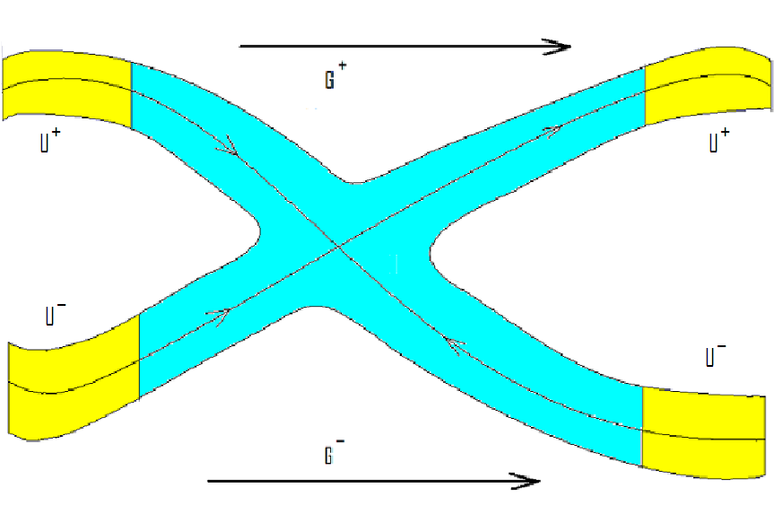
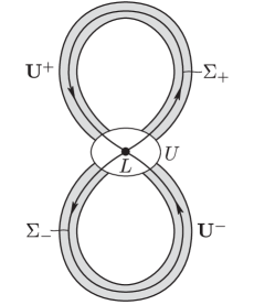
Figure 4: Gluing maps.

4 Normal forms

4.1 Moser normal form close to the torus

We start, as in [Tre02], by performing the classical Moser normal form [Mos56] to the unperturbed Hamiltonian $H_{0}$. To obtain a finitely smooth version of this result we apply a result in [BdlLW96].

Lemma 4.1.

Let $H_{0}$ is $\mathcal{C}^{r}$ satisfying [H1^′] and [H2]. For $I\in\mathcal{D}$ and $(p,q)$ close to $(0,0)$ there exists a system of coordinates $(I,s,x,y)$ such that

• the change $\mathcal{F}_{0}:(I,s,x,y)\longrightarrow(I,\varphi,p,q)$ $\mathcal{C}^{\ell}$ smooth and symplectic with $\ell\geq(r-4)/5$.

• in the variables $H_{0}\circ\mathcal{F}_{0}=\mathcal{H}_{0}(I,xy)$ is $\mathcal{C}^{\ell+1}$ smooth. We write it as

  $$\mathcal{H}_{0}(I,xy)=E(I)+g(I,xy)$$

  where $g(I,xy)=\lambda(I)xy+\mathcal{O}_{2}(xy)$.

Proof.

In Lemma 1,[Tre02] the assumption is that $H_{0}$ is analytic in $p,q$. To relax this assumption we use Theorem 1.1 [BdlLW96]. Recall that by Remark 1.1 we can assume that the saddle is at $(p,q)=(0,0)$ for all $I$ at the expense of loosing two derivatives.

Let $f$ be a $\mathcal{C}^{r-2}$ diffeomorphism with the fixed point at the origin $f(0)=0$. Let $N$ be a symplectic polynomial map such that $N(0)=0$ and the $k$-jet of $f$ and $N$ coincide at $0$, i.e. $D^{j}f(0)=D^{j}N(0),\ j=0,\dots,k$. Let $1\leq\ell<kA-B$ and $r-2>2k+4$ for some integer $\ell$. Then $N$ and $f$ are $\mathcal{C}^{\ell}$ conjugate, i.e. there is a $\mathcal{C}^{\ell}$ diffeomorphism $h$ such that $h^{-1}\circ f\circ h=N$ near the origin, $h(0)=0$.

In our case for each fixed $I$ we have a $2$-dimensional symplectic map $f$ with a saddle fixed point. By the remark after Theorem 1.1 of [BdlLW96], $A=1/4,\ B=1-2A=1/2$. Thus, $1\leq\ell<\frac{k-2}{4}<\frac{r-10}{8}$. ∎

We consider the expansion in $\varepsilon$ of the perturbation of the Hamiltonian (2), namely,

$$H_{1}=H_{11}+\varepsilon H_{12}+\mathcal{O}(\varepsilon^{2})$$

and define

$$\mathcal{H}_{\varepsilon}=\mathcal{H}_{0}+\varepsilon\mathcal{H}_{1}+\varepsilon^{2}\mathcal{H}_{2}+\mathcal{O}(\varepsilon^{3})$$ (22)

with

$$\mathcal{H}_{1}(I,s,x,y,t)=H_{11}\circ(\mathcal{F}_{0}(I,s,x,y),t),\quad\mathcal{H}_{2}(I,s,x,y,t)=H_{12}\circ(\mathcal{F}_{0}(I,s,x,y),t).$$

Since we assume that $r/8-5/4\geq s$ we have that $\mathcal{H}^{0}$ is $\mathcal{C}^{s+1}$, $\mathcal{H}_{1}$ is $\mathcal{C}^{s}$ and $\mathcal{H}_{2}$ is $\mathcal{C}^{s-1}$. Moreover $\mathcal{O}(\varepsilon^{3})=\mathcal{O}_{\mathcal{C}^{s-2}}(\varepsilon^{3})$.

4.2 Normal forms near the separatrices

We extend the Moser normal form to the region where $|xy|$ is small (see the shaded/colored region Fig. 4 on the right/left respectively). This normal form applies to both the non-resonant and resonant regimes. Since we want to make a second order analysis of the separatrix map we need a more precise normal form than in [Tre02]. In this normal form there are two sources of error.

• Expansion in the small parameter $\varepsilon$: we need to perform two steps of normal form instead of one to reduce the size of the remainders.

• Powers of $xy$: Treschev only performs normal form to remove the terms in the perturbation which are independent of the product $xy$. He takes

  $$\varepsilon^{5/4}|\log\varepsilon|\lesssim|xy|\lesssim\varepsilon^{7/8}.$$

  We want to remove terms up to the first order in $xy$. Assume that

  $$\varepsilon^{1+a}\lesssim|xy|\lesssim\varepsilon\qquad\text{with }1\geq a\geq 0.$$ (23)

We perform the change of coordinates by the Lie Method. First, we proceed formally and then we compute the estimates. We consider the expansion of the Hamiltonian $\mathcal{H}$ given in (22) and of a Hamiltonian of the form $\varepsilon W=\varepsilon W_{0}+\varepsilon^{2}W_{1}$. Call $\Phi$ the time-one map associated to the flow of $\varepsilon W$. This change is symplectic. Moreover,

$$\begin{split}\mathcal{H}_{\varepsilon}\circ\Phi=&\mathcal{H}_{\varepsilon}+\varepsilon\{\mathcal{H},W\}+\varepsilon^{2}\{\{\mathcal{H},W\},W\}+\mathcal{O}\left(\varepsilon^{3}\right)\\ =&\mathcal{H}_{0}+\varepsilon\left(\mathcal{H}_{1}+\{\mathcal{H}_{0},W_{0}\}\right)\\ &+\varepsilon^{2}\left(\{\mathcal{H}_{0},W_{1}\}+\{\mathcal{H}_{1},W_{0}\}+\{\{\mathcal{H}_{0},W_{0}\},W_{0}\}+\mathcal{H}_{2}\right)+\mathcal{O}\left(\varepsilon^{3}\right).\end{split}$$

Now we look for suitable $W_{0}$ and $W_{1}$.

First, compute $W_{0}$ and then $W_{1}$. To compute $W_{0}$, split the Hamiltonian $\mathcal{H}_{1}$, defined in (22), in the following way

$$\begin{split}\mathcal{H}_{1}(I,s,x,y,t)=&\,\overline{\bf H}_{1}(I,s,t)+\mathcal{H}^{(1)}(I,s,t)+\mathcal{H}^{(2)}(I,s,y,t)+\mathcal{H}^{(3)}(I,s,x,t)\\ +&xy\left(\overline{\bf H}_{2}(I,s,t)+\mathcal{H}^{(4)}(I,s,t)+\mathcal{H}^{(5)}(I,s,y,t)+\mathcal{H}^{(6)}(I,s,y,t)\right)\\ +&\mathcal{O}^{*}_{2}(xy)\end{split}$$

where

$$\overline{\bf H}_{2}(I,s,t)=\sum_{k\in\mathbb{Z}^{n+1}}\psi\left(\frac{k\cdot(\nu(I),1)}{\beta}\right)\partial_{xy}H_{1}^{k}(I,0,0)e^{2\pi ik\cdot(s,t)},$$ (24)

$\psi$ is the bump function introduced before (4) and

$$\begin{split}\mathcal{H}_{1}^{(1)}(I,s,t)&=\mathcal{H}_{1}(I,s,0,0,t)-\overline{\bf H}_{1}(I,s,t)\\ \mathcal{H}_{1}^{(2)}(I,s,t)&=\mathcal{H}_{1}(I,s,x,0,t)-\mathcal{H}_{1}(I,s,0,0,t)\\ \mathcal{H}_{1}^{(3)}(I,s,t)&=\mathcal{H}_{1}(I,s,0,y,t)-\mathcal{H}_{1}(I,s,0,0,t)\\ \mathcal{H}_{1}^{(4)}(I,s,t)&=\partial_{xy}\mathcal{H}_{1}(I,s,0,0,t)-\overline{\bf H}_{2}(I,s,t)\\ \mathcal{H}_{1}^{(5)}(I,s,t)&=\partial_{xy}\mathcal{H}_{1}(I,s,x,0,t)-\partial_{xy}\mathcal{H}_{1}(I,s,0,0,t)\\ \mathcal{H}_{1}^{(6)}(I,s,t)&=\partial_{xy}\mathcal{H}_{1}(I,s,0,y,t)-\partial_{xy}\mathcal{H}_{1}(I,s,0,0,t),\\ \end{split}$$ (25)

where $\overline{\bf H}_{1}$ is defined in (4). The functions $\overline{\bf H}_{1}$, $\mathcal{H}_{1}^{(j)}$, $j=1,2,3$ are $\mathcal{C}^{s}$ whereas the functions $\mathcal{H}_{1}^{(j)}$, $j=4,5,6$ are $\mathcal{C}^{s-2}$.

The next lemma contains the first step of the normal form. In the next two lemmas we denote by $\{\cdot,\cdot\}_{(x,y)}$, the Poisson bracket with respect to the conjugate variables $(x,y)$.

Lemma 4.2.

There exists a $\mathcal{C}^{s-2}$ smooth solution $W_{0}(I,s,x,y,t)$ of the equation

$$\left(\nu(I)+\partial_{I}g(I,xy)\right)\partial_{s}W_{0}+\partial_{t}W_{0}+\{g(I,xy),W_{0}\}_{(x,y)}+\sum_{j=1}^{3}\mathcal{H}_{1}^{(j)}+xy\sum_{j=4}^{6}\mathcal{H}_{1}^{(j)}=0.$$

The functions $W_{0}$ satisfies

$$W_{0}=\mathcal{O}^{*}(\beta^{-1}),$$

where $\mathcal{O}^{*}$ is defined in (5).

Proof.

We take $W_{0}=\sum_{j=1}^{6}W_{0}^{(j)}$ and solve the equations

$$\begin{split}\left(\nu(I)+\partial_{I}g(I,xy)\right)\partial_{s}W_{0}^{j}+\partial_{t}W_{0}^{j}+\{g(I,xy),W_{0}^{j}\}_{(x,y)}+\mathcal{H}_{1}^{(j)}&=0,\ j=1,2,3\ \\ \left(\nu(I)+\partial_{I}g(I,xy)\right)\partial_{s}W_{0}^{j}+\partial_{t}W_{0}^{j}+\{g(I,xy),W_{0}^{j}\}_{(x,y)}+xy\mathcal{H}_{1}^{(j)}&=0,\ j=4,5,6.\end{split}$$

Each equation is solved as follows. For the first and fourth ones, we just have

$$\begin{split}\left(\nu(I)+\partial_{I}g(I,xy)\right)\partial_{s}W_{0}^{1}+\partial_{t}W_{0}^{1}+\mathcal{H}_{1}^{(1)}&=0\\ \left(\nu(I)+\partial_{I}g(I,xy)\right)\partial_{s}W_{0}^{4}+\partial_{t}W_{0}^{4}+xy\mathcal{H}_{1}^{(4)}&=0.\end{split}$$

Thus, we invert the operator

$$\widetilde{\partial}:=(\nu(I)+\partial_{I}g(I,xy))\partial_{s}+\partial_{t}$$ (26)

by using the Fourier expansion and inverting for each Fourier coefficient. Note that this operator and the operator $\partial$ in (13) satisfy $\widetilde{\partial}-\partial=\mathcal{O}(xy)$. Moreover, recall that $\mathcal{H}_{0}$ is $\mathcal{C}^{s+1}$ and therefore so is $g$. Then, $W_{0}^{1,4}$ are $\mathcal{C}^{s-2}$ and satisfy

$$W_{0}^{1}=\partial^{-1}\mathcal{H}_{1}^{(1)}=\mathcal{O}^{*}(\beta^{-1})\ \text{ and }\ W_{0}^{4}=\mathcal{O}^{*}(xy\beta^{-1}).$$

For the others, we use the characteristics method to obtain

$$\begin{split}W_{0}^{2}&=-\int_{-\infty}^{0}\mathcal{H}_{1}^{(2)}(I,s+(\nu(I)+\partial_{I}g(I,xy))t^{\prime},ye^{\partial_{2}g(I,xy)t^{\prime}},t+t^{\prime})\,dt^{\prime}\\ W_{0}^{3}&=-\int^{+\infty}_{0}\mathcal{H}_{1}^{(3)}(y,s+(\nu(I)+\partial_{I}g(I,xy))t^{\prime},xe^{-\partial_{2}g(I,xy)t^{\prime}},t+t^{\prime})\,dt^{\prime}\\ W_{0}^{5}&=-xy\int_{-\infty}^{0}\mathcal{H}_{1}^{(5)}(I,s+(\nu(I)+\partial_{I}g(I,xy))t^{\prime},ye^{\partial_{2}g(I,xy)t^{\prime}},t+t^{\prime})\,dt^{\prime}\\ W_{0}^{6}&=xy\int^{+\infty}_{0}\mathcal{H}_{1}^{(6)}(I,s+(\nu(I)+\partial_{I}g(I,xy))t^{\prime},xe^{-\partial_{2}g(I,xy)t^{\prime}},t+t^{\prime})\,dt^{\prime}.\end{split}$$

Thus, they are all $\mathcal{C}^{s-2}$. ∎

Now we solve the second order equation. Define

$$\widetilde{\mathcal{H}}_{2}=\{\mathcal{H}_{1},W_{0}\}+\{\{\mathcal{H}_{0},W_{0}\},W_{0}\}+\mathcal{H}_{2},$$

where $\mathcal{H}_{2}$ is Hamiltonian defined in (22). Using the equation for $W_{0}$, given in Lemma 4.2, one has that $\widetilde{\mathcal{H}}_{2}$ is $\mathcal{C}^{s-3}$.

Let $\widetilde{\mathcal{H}}_{2}^{k}(I,0,0),\ k\in\mathbb{Z}^{n+1}$ denote the Fourier coefficients of $\mathcal{H}_{2}$ in $s$ and $t$. We split $\widetilde{\mathcal{H}}_{2}$ in several terms, as done for $\mathcal{H}^{1}$, in the following way

$$\begin{split}\widetilde{\mathcal{H}}_{2}(I,s,x,y,t)=&\,\overline{\bf H}_{3}(I,s,t)+\mathcal{H}_{2}^{(1)}(I,s,t)+\mathcal{H}_{2}^{(2)}(I,s,y,t)+\mathcal{H}_{2}^{(3)}(I,s,x,t)\\ &+\mathcal{O}^{*}(xy)\end{split}$$

with

$$\overline{\bf H}_{3}(I,s,t)=\sum_{k\in\mathbb{Z}^{n+1}}\psi\left(\frac{k\cdot(\nu(I),1)}{\beta}\right)\widetilde{\mathcal{H}}_{2}^{k}(I,0,0)e^{2\pi ik\cdot(s,t)}$$ (27)

and

$$\begin{split}\mathcal{H}_{2}^{(1)}(I,s,t)&=\widetilde{\mathcal{H}}_{2}(I,s,0,0,t)-\overline{\bf H}_{3}(I,s,t)\\ \mathcal{H}_{2}^{(2)}(I,s,t)&=\widetilde{\mathcal{H}}_{2}(I,s,x,0,t)-\widetilde{\mathcal{H}}_{2}(I,s,0,0,t)\\ \mathcal{H}_{2}^{(3)}(I,s,t)&=\widetilde{\mathcal{H}}_{2}(I,s,0,y,t)-\widetilde{\mathcal{H}}_{2}(I,s,0,0,t).\end{split}$$

All these terms are $\mathcal{C}^{s-3}$.

Lemma 4.3.

There exists a $\mathcal{C}^{s-3}$ smooth solution $W_{1}(I,s,x,y,t)$ of the equation

$$\left(\nu(I)+\partial_{I}g(I,xy)\right)\partial_{s}W_{1}+\partial_{t}W_{1}+\{g(I,xy),W_{1}\}_{(x,y)}+\sum_{j=1}^{3}\mathcal{H}_{2}^{(j)}=0.$$

Moreover, $W_{1}=\mathcal{O}^{*}(\beta^{-3})$, where $\mathcal{O}^{*}$ is defined in (5).

Proof.

As in the proof of Lemma 4.2, we take $W_{1}=\sum_{j=1}^{3}W_{1}^{(j)}$ and solve the equations

$$\left(\nu(I)+\partial_{I}g(I,xy)\right)\partial_{s}W_{1}^{j}+\partial_{t}W_{1}^{j}+\{g(I,xy),W_{1}^{j}\}_{(x,y)}+\mathcal{H}_{2}^{(j)}=0,\quad j=1,2,3.$$

Each equation is solved in the same way as the first order in Lemma 4.2. One can see that $\widetilde{\mathcal{H}}_{2}$ satisfies $\widetilde{\mathcal{H}}_{2}=\mathcal{O}^{*}(\beta^{-2})$. This implies that $W_{1}=\mathcal{O}^{*}(\beta^{-3})$ (one can have more precise bounds for each $W_{1}^{j}$). ∎

Denote by

$$\Phi:(\widehat{I},\widehat{s},\widehat{x},\widehat{y},\widehat{t})\ \longmapsto\ (I,s,x,y,t)$$

the time-one map associated to the flow of the Hamiltonian $\varepsilon W=\varepsilon W_{0}+\varepsilon^{2}W_{1}$. This change is $\mathcal{C}^{s-4}$ and symplectic. In the next two lemmas we analyze the change of coordinates and the transformed Hamiltonian.

Lemma 4.4.

The change $\Phi$ is $\mathcal{C}^{s-4}$ and satisfies the equations

$$\begin{split}I=&\,\widehat{I}+\varepsilon M_{1}^{I}+\varepsilon^{2}M_{2}^{I}+\mathcal{O}^{*}\left(\varepsilon^{3}\beta^{-5}\right)\\ =&\,\widehat{I}+\varepsilon\partial_{s}W_{0}+\varepsilon^{2}\left(\partial_{s}W_{1}+\{\partial_{s}W_{0},W_{0}\}\right)+\mathcal{O}^{*}\left(\varepsilon^{3}\beta^{-5}\right)\\ s=&\,\widehat{s}+\varepsilon M_{1}^{s}-\varepsilon^{2}M_{2}^{s}+\mathcal{O}^{*}\left(\varepsilon^{3}\beta^{-6}\right)\\ =&\,\widehat{s}-\varepsilon\partial_{I}W_{0}-\varepsilon^{2}\left(\partial_{I}W_{1}+\{\partial_{I}W_{0},W_{0}\}\right)+\mathcal{O}^{*}\left(\varepsilon^{3}\beta^{-6}\right)\\ x=&\,\widehat{x}+\varepsilon M_{1}^{x}+\varepsilon^{2}M_{2}^{x}+\mathcal{O}^{*}\left(\varepsilon^{3}\beta^{-5}\right)\\ =&\,\widehat{x}+\varepsilon\partial_{y}W_{0}+\varepsilon^{2}\left(\partial_{y}W_{1}+\{\partial_{y}W_{0},W_{0}\}\right)+\mathcal{O}^{*}\left(\varepsilon^{3}\beta^{-5}\right)\\ y=&\,\widehat{y}+\varepsilon M_{1}^{y}+\varepsilon^{2}M_{2}^{y}+\mathcal{O}^{*}\left(\varepsilon^{3}\beta^{-5}\right)\\ =&\,\widehat{y}-\varepsilon\partial_{x}W_{0}-\varepsilon^{2}\left(\partial_{x}W_{1}+\{\partial_{x}W_{0},W_{0}\}\right)-\mathcal{O}^{*}\left(\varepsilon^{3}\beta^{-5}\right)\end{split}$$

Moreover,

$$M_{1}^{z}=\mathcal{O}^{*}(\beta^{-1}),\,\,z=I,x,y\quad\text{ and }M_{1}^{s}=\mathcal{O}^{*}(\beta^{-2})$$

and

$$M_{2}^{z}=\mathcal{O}^{*}(\beta^{-3}),\,\,z=I,x,y\quad\text{ and }M_{2}^{s}=\mathcal{O}^{*}(\beta^{-4}).$$

We also have

$$xy=\widehat{x}\widehat{y}+\varepsilon M_{1}^{r}+\varepsilon^{2}M_{2}^{r}+\mathcal{O}^{*}\left(\varepsilon^{3}\beta^{-5}\right),$$

with

$$M_{1}^{r}=\mathcal{O}^{*}(\beta^{-1}),\quad\text{ and }M_{2}^{r}=\mathcal{O}^{*}(\beta^{-3}).$$

The inverse change is of the same form, that is

$$\begin{split}\widehat{I}=&I-\varepsilon M_{1}^{I}+\varepsilon^{2}\widetilde{M}_{2}^{I}+\mathcal{O}^{*}\left(\varepsilon^{3}\beta^{-5}\right)\\ \widehat{s}=&s-\varepsilon M_{1}^{s}-\varepsilon^{2}\widetilde{M}_{2}^{s}+\mathcal{O}^{*}\left(\varepsilon^{3}\beta^{-6}\right)\\ \widehat{x}=&x-\varepsilon M_{1}^{x}+\varepsilon^{2}\widetilde{M}_{2}^{x}+\mathcal{O}^{*}\left(\varepsilon^{3}\beta^{-5}\right)\\ \widehat{y}=&y-\varepsilon M_{1}^{y}+\varepsilon^{2}\widetilde{M}_{2}^{y}+\mathcal{O}^{*}\left(\varepsilon^{3}\beta^{-5}\right)\\ \end{split}$$

and

$$\widehat{x}\widehat{y}=xy-\varepsilon M_{1}^{r}+\varepsilon^{2}\widetilde{M}_{2}^{r}+\mathcal{O}^{*}(\beta^{-5}\varepsilon^{3}).$$

The terms $\widetilde{M}_{2}^{z}$ satisfy the same estimates as $M_{2}^{z}$.

Proof.

It is enough to recall that

$$\widehat{I}=I+\varepsilon\{I,W\}+\varepsilon^{2}\{\{I,W\},W\}+\ldots.$$

To compute the remainder, one has to estimate

$$\{\{\{z,W_{0}\},W_{0}\},W_{0}\}+\{\{z,W_{0}\},W_{1}\}+\{\{z,W_{1}\},W_{0}\},\qquad z=I,s,x,y.$$

Using the estimates for $W_{0}$ and $W_{1}$, one obtains the bounds for the remainder. ∎

Now we can apply this symplectic change of coordinates to the Hamiltonian $\mathcal{H}_{\varepsilon}$ given by Lemma 4.1.

Lemma 4.5.

The Hamiltonian $\mathcal{H}_{\varepsilon}\circ\Phi$ is $\mathcal{C}^{s-4}$ and is of the following form

$$\begin{split}\mathcal{H}_{\varepsilon}\circ\Phi(\widehat{I},\widehat{s},\widehat{x},\widehat{y},\widehat{t})=&E(\widehat{I}\,)+g(\widehat{I},\widehat{x}\widehat{y})+\varepsilon\overline{\bf H}_{1}(\widehat{I},\widehat{s},\widehat{t}\,)+\varepsilon\widehat{x}\widehat{y}\,\overline{\bf H}_{2}(\widehat{I},\widehat{s},\widehat{t}\,)\\ &+\varepsilon^{2}\,\overline{\bf H}_{3}(\widehat{I},\widehat{s},\widehat{t}\,)+\mathcal{O}^{*}\left(\varepsilon^{3}\beta^{-4}+\varepsilon^{2}\beta^{-2}\widehat{x}\widehat{y}+\varepsilon(\widehat{x}\widehat{y})^{2}\right).\end{split}$$

5 Transition near the singularity dynamics in the normal form

We compute the equation associated to the Hamiltonian given in Lemma 4.5. We drop the hats to simplify notation. Following [Tre02], consider a region for the initial conditions of the form

$$U_{*}=\left\{(I,s,x,y):c_{*}<|x|<c_{*}^{-1},\,c_{0}^{-1}(\varepsilon\beta^{-1}+|xy|)^{2}\log^{2}(xy)\leq|xy|\leq\kappa_{*}\right\}$$ (28)

and a final time $\overline{t}$ with

$$c_{*}\leq|y_{*}|\,e^{\partial_{1}g(I^{*},\rho)\overline{t}}\leq c_{*}^{-1}.$$

Take, as in [Tre02], $c^{*}$ and $c_{0}$ independent of $\varepsilon$ and $\kappa_{*}\sim\varepsilon$.

The Hamiltonian obtained in Lemma 4.5 has different formulas in non-resonant and resonant zones. We first analyze it in the non-resonant zone and later in the resonant one, which are defined in (16) and (17) respectively.

5.1 The non-resonant regime

Recall that we study trigonometric perturbations. In the non-resonant zone (16), analyzing (4), (24), and (27) we have that $\overline{\bf H}_{j}=0$ for $j=1,2,3$. Therefore, we have the Hamiltonian

$$\mathcal{H}_{\varepsilon}\circ\Phi(\widehat{I},\widehat{s},\widehat{x},\widehat{y},\widehat{t})=E(\,\widehat{I}\,)+g(\widehat{I},\widehat{x}\widehat{y})+\mathcal{O}^{*}\left(\varepsilon^{3}\beta^{-4}+\varepsilon^{2}\beta^{-2}\widehat{x}\widehat{y}+\varepsilon(\widehat{x}\widehat{y})^{2}\right),$$ (29)

which is $\mathcal{C}^{s-4}$ and is integrable up to order 3.

Lemma 5.1.

Suppose that for some $(I_{*},s_{*},x_{*},y_{*})\in U_{*}$ (see (28)) and $\overline{t}\in\mathbb{R}$,

$$c_{*}\leq|y_{*}|\,e^{\partial_{2}g(I,\rho)\overline{t}}\leq c_{*}^{-1}.$$

where $\rho=|x_{*}y_{*}|$.

Then,

$$\begin{split}s(\overline{t})&=\ s^{*}+\left(\nu(I^{*})+\partial_{I}g(I^{*},\rho)\right)\overline{t}+\mathcal{O}^{*}\left(\varepsilon^{3}\beta^{-5}+\varepsilon^{2}\beta^{-2}\rho+\varepsilon\rho^{2}\right)\log^{2}\rho\\ I(\overline{t})&=\ I^{*}+\mathcal{O}^{*}\left(\varepsilon^{3}\beta^{-4}+\varepsilon^{2}\beta^{-2}\rho+\varepsilon\rho^{2}\right)|\log\rho|\\ x(\overline{t})&=\ x_{*}e^{-\partial_{2}g(I^{*},\rho)\overline{t}}+\mathcal{O}^{*}\left(\varepsilon^{3}\beta^{-4}+\varepsilon^{2}\beta^{-2}\rho+\varepsilon\rho^{2}\right)\\ y(\overline{t})&=\ y_{*}e^{\,\partial_{2}g(I^{*},\rho)\overline{t}}\left(1+\mathcal{O}^{*}\left(\varepsilon^{3}\beta^{-4}+\varepsilon^{2}\beta^{-2}\rho+\varepsilon\rho^{2}\right)\right)\\ x(\overline{t})y(\overline{t})&=\ x^{*}y^{*}+\mathcal{O}^{*}\left(\varepsilon^{3}\beta^{-4}+\varepsilon^{2}\beta^{-2}\rho+\varepsilon\rho^{2}\right)|\log\rho|.\end{split}$$

Proof.

The proof of this lemma is a direct consequence of the particular form of the equations associated to Hamiltonian (29). Indeed, one can easily see that

$$\frac{d}{dt}(xy)=\mathcal{O}^{*}\left(\varepsilon^{3}\beta^{-4}+\varepsilon^{2}\beta^{-2}\widehat{x}\widehat{y}+\varepsilon(\widehat{x}\widehat{y})^{2}\right).$$

Therefore, one can easily see that

$$|x(\overline{t})y(\overline{t})-x^{*}y^{*}|=\mathcal{O}^{*}\left(\varepsilon^{3}\beta^{-4}+\varepsilon^{2}\beta^{-2}\rho+\varepsilon\rho^{2}\right)|\log\rho|.$$

Taking this into account, we have

$$\dot{I}=\mathcal{O}^{*}\left(\varepsilon^{3}\beta^{-4}+\varepsilon^{2}\beta^{-2}\rho+\varepsilon\rho^{2}\right)$$

which leads to the formula for $I(\overline{t})$. Using that $I$ is almost constant, one can easily deduce the formulas for the other variables. ∎

5.2 The resonant regime

To analyze the resonant regime recall that we focus on the case of two and a half degrees of freedom. Namely, $s\in\mathbb{T}$ and $I\in\mathbb{R}$. We perform a change to slow-fast variables. This leads to a Hamiltonian which is almost a first integral, namely, its time dependent terms are small.

Fix $(k_{0},k_{1})\in\mathbb{Z}^{2}$. Assume that the resonance $(\nu(I),1)\cdot(k_{0},k_{1})=0$, $(k_{0},k_{1})\in\mathcal{N}^{(2)}(H_{1})\subset\mathbb{Z}^{2}$ is located at $I=0$. Call $A$ the variable conjugate to time. Then, the change

$$(J,\theta,D,t)=\left(\frac{I}{k_{0}},k_{0}s+k_{1}t,A-\frac{k_{1}}{k_{0}}I,t\right)$$

is symplectic. Applying this change, one obtains the following Hamiltonian. We drop the hats to simplify notations.

$$\widetilde{\mathcal{H}}(J,\theta,x,y,t)=\widetilde{E}(J)+\widetilde{g}(J,xy)+\varepsilon\widetilde{\mathcal{H}}_{1}(J,\theta,xy)+\mathcal{O}^{*}\left(\varepsilon^{3}\beta^{-4}+\varepsilon^{2}\beta^{-2}xy+\varepsilon(xy)^{2}\right).$$

where

$$\widetilde{E}(J)=E(k_{0}J)+k_{1}J,$$

satisfies

$$\partial_{J}\widetilde{E}(0)=0,\ \ \ \widetilde{g}(J,xy)=g(k_{0}J,xy)$$

and

$$\widetilde{\mathcal{H}}_{1}(J,\theta,xy)=$$

$$\sum_{j=-N}^{N}\left(\overline{\bf H}_{1}^{(jk_{0},jk_{1})}(k_{0}J)+xy\,\overline{\bf H}_{2}^{(jk_{0},jk_{1})}(k_{0}J)+\varepsilon\,\overline{\bf H}_{3}^{(jk_{0},jk_{1})}(k_{0}J)\right)e^{2\pi ij\theta}.$$

We use this system of coordinates to analyze the flow in the resonant zones. Recall that by construction $\widetilde{\nu}(0)=0$. Since we consider $\beta>0$ fixed and in order to avoid cluttering the notation, from now on, we do not keep track of the $\beta$ dependence of each estimate. We also assume $\rho\lesssim\varepsilon$.

Lemma 5.2.

Suppose that for some $(J_{*},\theta_{*},x_{*},y_{*})\in U_{*}$ and $\overline{t}\in\mathbb{R}$,

$$c_{*}\leq|y_{*}|e^{\partial_{2}g(J_{*},\rho)\overline{t}}\leq c_{*}^{-1}.$$

where $\rho=|x_{*}y_{*}|$.

Then,

$$\begin{split}\theta(\overline{t})=&\theta^{*}+\left(\nu(J^{*})+\partial_{1}g(J^{*},\rho)\right)\overline{t}+\varepsilon F_{1}(J^{*},\theta^{*},\overline{t})+\mathcal{O}^{*}\left(\varepsilon^{11/6}\right)\\ J(\overline{t})=&J^{*}+\varepsilon G_{1}(J^{*},\theta^{*},\overline{t})+\mathcal{O}^{*}\left(\varepsilon^{11/6}\right)\\ x(\overline{t})=&x_{*}e^{-\left(\partial_{2}g(J^{*},\rho)\overline{t}+\varepsilon\Phi(J^{*},\theta^{*},\overline{t})\right)}+\mathcal{O}^{*}\left(\varepsilon^{11/6}\right)\\ y(\overline{t})=&y_{*}e^{\partial_{2}g(J^{*},\rho)\overline{t}+\varepsilon\Phi(J^{*},\theta^{*},\overline{t})}\left(1+\mathcal{O}^{*}\left(\varepsilon^{11/6}\right)\right)\\ x(\overline{t})y(\overline{t})=&x^{*}y^{*}+\mathcal{O}^{*}\left(\varepsilon^{5/2}\right),\end{split}$$

where

$$F_{1}(J,\theta,\overline{t}) =-\frac{\nu^{\prime}(J)}{\nu(J)}\sum_{k=-N,k\neq 0}^{N}H_{1}^{k}(J)e^{2\pi i\theta}\left(\overline{t}-\frac{e^{2\pi ik\nu(J)\overline{t}}-1}{2\pi ik\nu(J)}\right)$$ (30)

$$+\partial_{J}H_{1}(J)\overline{t}+\sum_{k=-N,k\neq 0}^{N}\frac{1}{2\pi ik\nu(J)}\partial_{J}H_{1}(J)e^{2\pi ik\theta}\left(e^{2\pi ik\nu(J)\overline{t}}-1\right)$$

$$G_{1}(J,\theta,\overline{t}) =\nu(J)^{-1}\left(\overline{\bf H}_{1}(J,\theta)-\overline{\bf H}_{1}(J,\theta+\nu(J)\overline{t})\right)$$ (31)

and

$$\Phi(J,\theta,\overline{t})=\int_{0}^{\overline{t}}\left(\overline{\bf H}_{2}(J,\theta+\nu(J)t)+\partial_{rJ}g(\rho,J)G_{1}(J,\theta,t)\right)dt.$$

Thus, $G$ has zero average with respect to $\theta$ and $F$ and $G$ satisfy

$$F=\mathcal{O}^{*}(\log\varepsilon)\qquad\text{ and }\qquad G=\mathcal{O}^{*}(1).$$

Proof.

From Lemma 4.5, we have the equations

$$\begin{split}\dot{\theta}=&\ \ \nu(J)+\partial_{J}g(J,xy)+\varepsilon\partial_{J}\overline{\bf H}_{1}(J,\theta)+\varepsilon xy\partial_{J}\overline{\bf H}_{2}(J,\theta)+\varepsilon^{2}\partial_{J}\overline{\bf H}_{3}(J,\theta)\\ &+\mathcal{O}^{*}\left(\varepsilon^{3}\beta^{-4}+\varepsilon^{2}\beta^{-2}xy+\varepsilon(xy)^{2}\right).\\ \dot{J}=&\ -\varepsilon\partial_{\theta}\overline{\bf H}_{1}(J,\theta)-\varepsilon xy\partial_{\theta}\overline{\bf H}_{2}(J,\theta)-\varepsilon^{2}\partial_{\theta}\overline{\bf H}_{3}(J,\theta)\\ &+\mathcal{O}^{*}\left(\varepsilon^{3}\beta^{-4}+\varepsilon^{2}\beta^{-2}xy+\varepsilon(xy)^{2}\right)\\ \dot{y}=&\ \ \partial_{r}g(J,xy)y+\varepsilon y\overline{\bf H}_{2}(J,\theta)+\mathcal{O}_{2}^{*}(\varepsilon\beta^{-1},xy)\\ \dot{x}=&\ -\partial_{r}g(J,xy)x+\varepsilon x\overline{\bf H}_{2}(J,\theta)+\mathcal{O}_{2}^{*}(\varepsilon\beta^{-1},xy).\end{split}$$

We also have

$$\frac{d}{dt}(xy)=\mathcal{O}^{*}\left(\varepsilon^{3}\beta^{-4}+\varepsilon^{2}\beta^{-2}xy+\varepsilon(xy)^{2}\right).$$

Now we compute estimates for this flow. Call $(I^{*},s^{*},q^{*},p^{*})$ to the initial point. Recall that $\rho=x^{*}y^{*}$, that we omit the dependence on $\beta$ and that we assume $\rho\lesssim\varepsilon$. Then,

$$|xy-x^{*}y^{*}|=\mathcal{O}^{*}\left(\varepsilon^{3}\log\varepsilon\right).$$ (32)

This implies that the first orders of $\dot{\theta}$ and $\dot{J}$ are independent of $x$ and $y$, since only depend on $\rho$. Indeed, we have

$$\begin{split}\dot{\theta}=&\nu(J)+\partial_{J}g(\rho,J)+\varepsilon\partial_{J}\overline{\bf H}_{1}(J,\theta)+\mathcal{O}^{*}(\varepsilon^{2})\\ \dot{J}=&-\varepsilon\partial_{\theta}\overline{\bf H}_{1}(J,\theta)+\mathcal{O}^{*}(\varepsilon^{2}).\end{split}$$

These equations can be solved perturbatively in powers of $\varepsilon$. We look formally for solutions of the following form and we take $t^{*}=0$

$$\begin{split}\theta(t)&=\theta^{*}+\nu(J^{*})t+\partial_{J}g(J^{*},\rho)t+\varepsilon F_{1}(J^{*},\theta^{*},t)+\text{h.o.t}\\ J(t)&=J^{*}+\varepsilon G_{1}(J^{*},\theta^{*},t)+\text{h.o.t}\end{split}$$

Plugging these expressions into the equation and recalling that $g(J^{*},\rho)=\partial_{J}g(J^{*},\rho)=\partial_{J}^{2}g(J^{*},\rho)=\mathcal{O}^{*}(\varepsilon)$, we obtain the following equations

$$\begin{split}\dot{F}_{1}=\,&\nu^{\prime}(J^{*})G_{1}+\partial_{J}\overline{\bf H}_{(}J^{*},\theta^{*}+\nu(J^{*})t)\\ \dot{G}_{1}=\,&-\partial_{\theta}\overline{\bf H}_{1}(J^{*},\theta^{*}+\nu(J^{*})t)\end{split}$$

We can first solve the second equation, taking

$$G_{1}(J^{*},\theta^{*},\overline{t})=-\int_{0}^{\overline{t}}\partial_{\theta}\overline{\bf H}_{1}(J^{*},\theta^{*}+\nu(J^{*})t)\,dt,$$

which leads to the formula of $G_{1}$ stated in the lemma.

Plugging the expression of $G_{1}$ into the $F_{1}$ equation , we obtain $F_{1}$,

$$\begin{split}F_{1}(J^{*},\theta^{*},\overline{t})=&-\nu^{\prime}(J^{*})\int_{0}^{\overline{t}}G_{1}(J^{*},\theta^{*},t)\,dt\\ &+\int_{0}^{\overline{t}}\partial_{J}\overline{\bf H}_{1}(J^{*},\theta^{*}+\nu(J^{*})t)\,dt.\end{split}$$

Now, expanding every term in Fourier series and integrating we get the formula for $F_{1}$. From their definition we can deduce that the functions $F_{1}$ and $G_{1}$ satisfy

$$F_{1}=\mathcal{O}^{*}\left(\log\varepsilon\right),\qquad G_{1}=\mathcal{O}^{*}\left(1\right).$$

Analyzing the remainders, one can easily compute the size of the higher order terms in the evolution of $J$ and $\theta$ given in Lemma 5.2.

Now we analyze the flow for the $x$ and $y$ variables. Recall that the conditions on the initial $y_{*}$ and on the time $\overline{t}$ imply

$$\frac{c_{*}^{2}}{\rho}\leq e^{\partial_{2}g(J^{*},\rho)\overline{t}}\leq\frac{1}{\rho c_{*}^{2}}.$$ (33)

Using the almost conservation of $xy$ and the formulas for $\theta(t)$ and $J(t)$, we have

$$\begin{split}\dot{y}=&\left(\partial_{r}g(\rho,J(t))+\varepsilon\overline{\bf H}_{2}(J(t),\theta(t))\right)y+\Theta_{1}(t)\\ \dot{x}=&-\left(\partial_{r}g(\rho,J(t))+\varepsilon\overline{\bf H}_{2}(J,\theta(t))\right)x+\Theta_{2}(t).\end{split}$$

where $\Theta_{i}=\mathcal{O}^{*}(\varepsilon^{2}\log\varepsilon)$.

Thus,

$$\begin{split}x(\overline{t})=&x_{*}e^{-\int_{0}^{\overline{t}}\left(\partial_{r}g(\rho,J(t))+\varepsilon\overline{\bf H}_{2}(J(t),\theta(t),t)\right)\,dt}\\ &+\int_{\sigma}^{\overline{t}}e^{-\int_{\sigma}^{\overline{t}}\left(\partial_{r}g(\rho,J(t))+\varepsilon\overline{\bf H}_{2}(J(t),\theta(t),t)\right)\,dt}\Theta_{1}(\sigma)\,d\sigma.\end{split}$$

Using (33),

$$x(\overline{t})=x_{*}e^{-\int_{0}^{\overline{t}}\left(\partial_{r}g(\rho,J(t))+\varepsilon\overline{\bf H}_{2}(J(t),\theta(t),t)\right)\,dt}+\mathcal{O}^{*}(\varepsilon^{2}\log^{2}\varepsilon).$$

Now we expand $J(t)$ and $\theta(t)$ with the formulas already obtained. Then,

$$x(\overline{t})=x_{*}e^{-\left(\partial_{r}g(\rho,J^{*})\overline{t}+\varepsilon\Phi(J^{*},\theta^{*},\overline{t})\right)}+\mathcal{O}^{*}(\varepsilon^{11/6})$$

with

$$\Phi(J^{*},\theta^{*},\overline{t})=\int_{0}^{\overline{t}}\left(\overline{\bf H}_{2}(J^{*},\theta^{*}+\nu(J^{*})t)+\partial_{rJ}g(\rho,J^{*})G_{1}(J^{*},\theta^{*},t)\right)dt.$$

Using this estimate and (32), we can deduce the following formulas for $y(\overline{t})$,

$$y(\overline{t})=y_{*}e^{\partial_{r}g(\rho,J^{*})\overline{t}+\varepsilon\Phi(J^{*},\theta^{*},\overline{t})}\left(1+\mathcal{O}^{*}(\varepsilon^{11/6})\right).$$

∎

6 The gluing maps

We compute the gluing maps. First in Section 6.1, we consider the unperturbed Hamiltonian $\mathcal{H}_{0}$ given in Lemma 4.1. Then, we consider the full Hamiltonian in the non-resonant setting (Section 6.2) and resonance setting (Section 6.3).

6.1 Unperturbed gluing maps

The unperturbed gluing maps are computed in Section 5 of [Tre02]. Consider the gluing maps

$$\begin{split}\mathcal{S}^{+}:&\{|y|\text{ is small},x>0\}\longrightarrow\{y>0,|x|\text{ is small}\}\\ \mathcal{S}^{-}:&\{|y|\text{ is small},x>0\}\longrightarrow\{y<0,|x|\text{ is small}\}.\end{split}$$ (34)

The gluing maps of the unperturbed system must satisfy the following properties

• are symplectic

• preserve $I$ and $xy$.

Lemma 6.1 ([Tre02]).

Properties (i), (ii) and (34) imply that the gluing maps

$$(I^{\pm},s^{\pm},x^{\pm},y^{\pm})=\mathcal{S}^{\pm}(I,s,x,y)$$

are of the form

$$\begin{split}I^{\pm}&=I\\ s^{\pm}&=s+\partial_{I}\Phi^{\pm}(I,xy)\\ y^{\pm}&=x^{-1}e^{-\partial_{r}\Phi^{\pm}(I,xy)}\\ x^{\pm}&=x^{2}ye^{\partial_{r}\Phi^{\pm}(I,xy)}\end{split}$$

for some functions $\Phi^{\pm}$.

In [Tre02] it is also shown that $\partial_{I}\Phi^{\pm}(I,r)=\mu^{\pm}(I)+\mathcal{O}(r)$ and $e^{\partial_{r}\Phi^{\pm}(I,r)}=\kappa^{\pm}(I)+\mathcal{O}(r)$. Notice that the maps $\mathcal{S}^{\pm}$ are $\mathcal{C}^{s}$.

Moreover, since $\rho=xy$, $x^{\pm}=\mathcal{O}(\rho)$ are always small. One can consider also the inverse change for $(x,y)$. Since $xy=x^{\pm}y^{\pm}$, it is given by

$$\begin{split}y&=y^{\pm}\rho e^{-\partial_{r}\Phi^{\pm}(I,\rho)}\\ x&=(y^{\pm})^{-1}e^{\partial_{r}\Phi^{\pm}(I,\rho)}.\end{split}$$

So, $y$ also is small since $y=\mathcal{O}(\rho)$.

6.2 Gluing maps in non-resonant zones

Now we express these gluing maps in the normal form coordinates $(\widehat{I},\widehat{s},\widehat{x},\widehat{y})$. We use the formulas for the normal form coordinates obtained in Section 4.2.

The gluing maps have the following form. Each term can be expressed in terms of the Hamiltonian $W$ associated to the normal form variables from Section 4.2.

$$\begin{split}\widehat{I}^{\pm}=&\widehat{I}+\varepsilon(M_{1}^{I}\circ\mathcal{S}^{\pm}-M_{1}^{I})+\varepsilon^{2}(M_{2}^{I}\circ\mathcal{S}^{\pm}-\widetilde{M}_{2}^{I})+\mathcal{O}^{*}(\varepsilon^{3}\beta^{-5})\\ \widehat{s}^{\pm}=&\widehat{s}+\partial_{I}\Phi^{\pm}(I+\varepsilon(M_{1}^{I}\circ\mathcal{S}^{\pm}-M_{1}^{I}),\widehat{x}\widehat{y}+\varepsilon(M_{1}^{r}\circ\mathcal{S}^{\pm}-M_{1}^{r}))\\ &+\varepsilon(M_{1}^{s}\circ\mathcal{S}^{\pm}-M_{1}^{s})+\mathcal{O}^{*}(\varepsilon^{2}\beta^{-4})\\ \widehat{y}^{\pm}=&\widehat{x}^{-1}e^{-\partial_{r}\Phi^{\pm}(\widehat{I},\widehat{x}\widehat{y})}+\mathcal{O}^{*}(\varepsilon\beta^{-1})\\ \widehat{x}^{\pm}=&e^{\partial_{r}\Phi^{\pm}(\widehat{I},\widehat{x}\widehat{y})}\widehat{x}\left(\widehat{x}\widehat{y}+\varepsilon(M_{1}^{r}\circ\mathcal{S}^{\pm}-M_{1}^{r})\right)+\mathcal{O}^{*}(\rho^{2}+\rho\varepsilon\beta^{-1}+\varepsilon^{2}\beta^{-3})\end{split}$$

Moreover,

$$\widehat{y}^{\pm}\widehat{x}^{\pm}=\widehat{y}\widehat{x}+\varepsilon(M_{1}^{r}\circ\mathcal{S}^{\pm}-M_{1}^{r})+\varepsilon^{2}(M_{2}^{r}\circ\mathcal{S}^{\pm}-\widetilde{M}_{2}^{r})+\mathcal{O}^{*}(\varepsilon^{3}\beta^{-5}).$$

6.3 Gluing maps in resonances

We consider the slow-fast variables $(\theta,J,x,y)$. In these variables, we have the gluing map

$$(J^{\pm},\theta^{\pm},y^{\pm},x^{\pm})=\mathcal{S}^{\pm}(J,\theta,x,y)$$

with

$$\begin{split}J^{\pm}&=J\\ \theta^{\pm}&=\theta+\partial_{J}\widetilde{\Phi}^{\pm}(J,xy)\\ y^{\pm}&=x^{-1}e^{-\partial_{r}\widetilde{\Phi}^{\pm}(J,xy)}\\ x^{\pm}&=x^{2}ye^{\partial_{r}\widetilde{\Phi}^{\pm}(J,xy)}\\ \end{split}$$

where

$$\widetilde{\Phi}^{\pm}(I,r)=\Phi^{\pm}(k_{0}I,r).$$

From now on, we drop the tilde in $\Phi^{\pm}$ to simplify the notation. We also abuse notation and we consider the normal form change of coordinates given by the generating function $W$ expressed in slow-fast variables (recall that all these changes of coordinates are symplectic).

Now we express the gluing map in the normal form (slow-fast) coordinates. As before, for the first four coordinates we have

$$\begin{split}\widehat{J}\pm=&\widehat{J}+\varepsilon(M_{1}^{J}\circ\mathcal{S}^{\pm}-M_{1}^{J})+\mathcal{O}^{*}(\varepsilon^{2})\\ \widehat{\theta}^{\pm}=&\widehat{\theta}+\partial_{J}\Phi^{\pm}(J+\varepsilon(M_{1}^{J}\circ\mathcal{S}^{\pm}-M_{1}^{J}),\widehat{x}\,\widehat{y}+\varepsilon(M_{1}^{r}\circ\mathcal{S}^{\pm}-M_{1}^{r}))\\ &+\varepsilon(M_{1}^{\theta}\circ\mathcal{S}^{\pm}-M_{1}^{\theta})+\mathcal{O}^{*}(\varepsilon^{2})\\ \widehat{y}^{\pm}=&\widehat{x}^{-1}e^{-\partial_{r}\Phi^{\pm}(J,\widehat{x}\,\widehat{y})}+\mathcal{O}^{*}(\varepsilon)\\ \widehat{x}^{\pm}=&e^{\partial_{r}\Phi^{\pm}(J,\widehat{x}\widehat{y})}\widehat{x}\left(\widehat{x}\widehat{y}+\varepsilon(M_{1}^{r}\circ\mathcal{S}^{\pm}-M_{1}^{r})\right)+\mathcal{O}^{*}(\varepsilon^{2})\end{split}$$

and

$$\widehat{y}^{\pm}\widehat{x}^{\pm}=\widehat{y}\,\widehat{x}+\varepsilon(M_{1}^{r}\circ\mathcal{S}^{\pm}-M_{1}^{r})+\varepsilon^{2}(M_{2}^{r}\circ\mathcal{S}^{\pm}-\widetilde{M}_{2}^{r})+\mathcal{O}_{3}^{*}(\varepsilon).$$

7 The separatrix map in the non-resonant regime

We use the results in Sections 5.1 and 6.2 to look for formulas of the separatrix map in the non-resonant regime (16). First we compose the flow in normal form coordinates and the gluing map. We obtain the separatrix map in the $(I,s,y,x)$ coordinates. Later we look for a good system of coordinates which will transform $(y,x)$ to a certain symplectic flow-box coordinates around the former separatrix.

Consider the flow $g_{\varepsilon}^{\overline{t}}$ analyzed in Lemma 5.1 and the gluing map analyzed in Section 6.2. We have the following

Lemma 7.1.

The composition of the two maps $\mathcal{F}=g_{\varepsilon}^{\overline{t}}\circ G_{\varepsilon}^{\sigma}$ is given by

$$\mathcal{F}(I,s,y,x)=(\mathcal{F}_{I}(I,s,y,x),\mathcal{F}_{s}(I,s,y,x),\mathcal{F}_{y}(I,s,y,x),\mathcal{F}_{x}(I,s,y,x))$$

with

$$\begin{split}\mathcal{F}_{I}=&I+\varepsilon\mathcal{P}_{1}^{I}+\varepsilon^{2}\mathcal{P}_{2}^{I}+\mathcal{O}^{*}(\varepsilon^{3}\beta^{-4}+\varepsilon^{2}\beta^{-2}\rho+\varepsilon\rho^{2})|\log\rho|\\ \mathcal{F}_{s}=&s+\partial_{I}\Phi^{\pm}(I,xy)+(\nu(I)+\partial_{I}g(I,xy))\overline{t}+\varepsilon\mathcal{P}_{1}^{s}+\mathcal{O}^{*}(\varepsilon^{2}\beta^{-4})|\log\rho|\\ \mathcal{F}_{y}=&x^{-1}\exp(-\partial_{r}g(I+\varepsilon\mathcal{P}_{1}^{I},xy+\varepsilon\mathcal{P}_{1}^{r})\overline{t}-\partial_{r}\Phi^{\pm}(I,xy))\times\\ &\left(1+\mathcal{O}_{2}^{*}(\varepsilon,\rho)|\log\rho|\right)+\mathcal{O}_{3}^{*}(\varepsilon,\rho)\\ \mathcal{F}_{x}=&\exp(\partial_{r}g(I+\varepsilon\mathcal{P}_{1}^{I},xy+\varepsilon\mathcal{P}_{1}^{r})\overline{t}+\partial_{r}\Phi^{\pm}(I,xy)))\times\\ &x(xy+\varepsilon\mathcal{P}_{1}^{r})\left(1+\mathcal{O}_{2}(\varepsilon,\rho)|\log\rho|\right),\end{split}$$

where

$$\begin{split}\mathcal{P}^{I}_{1}=&M_{1}^{I}\circ\mathcal{S}^{\pm}-M_{1}^{I}\\ \mathcal{P}^{I}_{2}=&M_{2}^{I}\circ\mathcal{S}^{\pm}-\widetilde{M}_{2}^{I}\end{split}$$

and

$$\begin{split}\mathcal{P}^{s}_{1}&=M_{1}^{s}\circ\mathcal{S}^{\pm}-M_{1}^{s}+\partial_{I}^{2}\Phi^{\pm}(I,xy)\left(M_{1}^{I}\circ\mathcal{S}^{\pm}-M_{1}^{I}\right)+\\ &+\partial^{2}_{r\,I}\Phi^{\pm}(I,xy)\left(M_{1}^{r}\circ\mathcal{S}^{\pm}-M_{1}^{r}\right)+\overline{t}\partial_{I}(\nu(I)+\partial_{I}g(I,xy))\left(M_{1}^{I}\circ\mathcal{S}^{\pm}-M_{1}^{I}\right)\\ &+\overline{t}\,\partial^{2}_{r\,I}g(I,xy)\left(M_{1}^{r}\circ\mathcal{S}^{\pm}-M_{1}^{r}\right)\end{split}$$

Moreover,

$$\mathcal{F}_{x}\mathcal{F}_{y}=xy+\varepsilon\mathcal{P}^{r}_{1}+\varepsilon^{2}\mathcal{P}^{r}_{2}+\mathcal{O}^{*}_{3}\left(\varepsilon\beta^{-1},\rho\right),$$

where

$$\begin{split}\mathcal{P}^{r}_{1}=&M_{1}^{r}\circ\mathcal{S}-M_{1}^{r}\\ \mathcal{P}^{r}_{2}=&M_{2}^{r}\circ\mathcal{S}-\widetilde{M}_{2}^{r}\end{split}$$

Then,

$$\mathcal{P}_{1}^{I},\mathcal{P}_{1}^{r}=\mathcal{O}^{*}(\beta^{-1}),\quad\mathcal{P}^{I}_{2},\mathcal{P}_{2}^{r}=\mathcal{O}^{*}(\beta^{-3}),\quad\text{and}\quad\mathcal{P}_{1}^{s}=\mathcal{O}^{*}(1)|\log\rho|.$$

The proof of this lemma is a direct consequence of the results in Lemma 5.1 and Section 6.2.

We look for a coordinate change near the former separatrix such that formulas for the separatrix map are as simple as possible. In comparison with [Tre02], we want to point out two main differences. First, since we are away from resonances, we have ${\bf\overline{H}}_{j}=0,\ j=1,2,3$. This simplifies the formulas. On the other hand, we want to have a more precise dependence on $xy$ since we are doing a higher order analysis. This second fact implies that we have to slightly modify the change of coordinates.

We look for a symplectic change

$$\left(\begin{split}s\\ I\\ y\\ x\end{split}\right)=\Upsilon\left(\begin{split}\xi\\ \eta\\ \tau\\ h\end{split}\right)$$

The function $I\mapsto g(I,r)$ introduced in Lemma 4.1 is invertible with respect to $r$ in a neighborhood of $r=0$ (recall that $\partial_{r}g(I,0)=\lambda(I)>0$, see Lemma 4.1). We have denoted by $g_{r}^{-1}(I,r)$ the inverse function with respect to the second coordinate $r$. We consider the following generating function.

$$\mathcal{S}(\eta,s,h,y)=\eta s+g_{r}^{-1}(\eta,h-E(\eta))\log|y|.$$ (35)

This generating function induces the following change of coordinates

$$\begin{pmatrix}\xi\\ \eta\\ \tau\\ h\end{pmatrix}=\begin{pmatrix}s-\partial_{r}g_{r}^{-1}(I,g(I,xy))(\nu(I)+\partial_{I}g(I,xy))\log|y|\\ I\\ \frac{\log|y|}{\partial_{r}g(I,xy)}\\ E(I)+g(I,xy)\end{pmatrix}$$

and

$$\begin{pmatrix}s\\ I\\ y\\ x\end{pmatrix}=\Upsilon\begin{pmatrix}\xi\\ \eta\\ \tau\\ h\end{pmatrix}=\begin{pmatrix}\xi+[\nu(\eta)+\partial_{\eta}g^{-1}(\eta,g_{r}^{-1}(h-E(\eta)))]\tau\\ \eta\\ \sigma\,\exp(\frac{\tau}{\partial_{r}g_{r}^{-1}(\eta,h-E(\eta))})\\ g_{r}^{-1}(\eta,h-E(\eta))\,\sigma\,\exp(-\frac{\tau}{\partial_{r}g_{r}^{-1}(\eta,h-E(\eta))})\end{pmatrix}$$ (36)

Note that the $y$ component does not get modified by this change of coordinates and that this change of coordinates does not depend on $\varepsilon$.

We express the separatrix map in these coordinates. We use the change $\Upsilon$ to write down the formulas. From now on we omit the dependence on $\beta$. Recall that $\beta>0$ is a fixed parameter independent of $\varepsilon$. Due to the previous analysis, smoothness of the separatrix map obeys the estimate in Theorem 3.1.

Lemma 7.2.

The separatrix map, has the following form

$$\begin{split}\eta^{*}=&\eta+\varepsilon\mathcal{P}_{1}^{I}\circ\Upsilon+\varepsilon^{2}\mathcal{P}_{2}^{I}\circ\Upsilon+\mathcal{O}_{3}^{*}(\varepsilon,\rho)|\log\rho|\\ \xi^{*}=&\xi+\partial_{I}\Phi^{\pm}(\eta,g_{r}^{-1}(\eta,h-E(\eta)))-\frac{\nu(\eta)+\partial_{I}g(\eta,g_{r}^{-1}(\eta,h-E(\eta)))}{\partial_{r}g(\eta,g_{r}^{-1}(\eta,h-E(\eta))}\log R\\ &+\mathcal{O}_{1}^{*}(\varepsilon+\rho)(|\log\varepsilon|+|\log\rho|)\\ h^{*}=&h+\varepsilon\left(\left[\nu(\eta)+\partial_{I}g(\eta,g_{r}^{-1}(\eta,h-E(\eta)))\right]\mathcal{P}_{1}^{I}\circ\Upsilon\right.\\ &\left.+\partial_{r}g(\eta,g_{r}^{-1}(\eta,h-E(\eta)))\mathcal{P}_{1}^{r}\circ\Upsilon\right)+\varepsilon^{2}\mathcal{P}_{2}^{h}+\mathcal{O}_{3}^{*}(\varepsilon,\rho)\\ \tau^{*}=&\tau+\overline{t}+\frac{1}{\partial_{r}g(\eta,g_{r}^{-1}(\eta,h-E(\eta))}\log R+\mathcal{O}_{1}^{*}(\varepsilon+\rho)(|\log\varepsilon|+|\log\rho|),\end{split}$$

where

$$R=e^{\partial_{r}\Phi^{\pm}(\eta,g_{r}^{-1}(\eta,h-E(\eta))}\left(g_{r}^{-1}(\eta^{*},h^{*}-E(\eta^{*}))+\mathcal{O}_{2}^{*}\right)$$ (37)

and

$$\begin{split}\mathcal{P}_{2}^{h}&=\left(\nu(\eta)+\partial_{I}g(\eta,g_{r}^{-1}(\eta,h-E(\eta)))\right)\mathcal{P}_{2}^{y}\circ\Upsilon\\ &+\partial_{r}g(\eta,g_{r}^{-1}(\eta,h-E(\eta)))\mathcal{P}_{2}^{r}\circ\Upsilon\\ &+\frac{1}{2}\left(\partial_{I}\nu(\eta)+\partial_{I}^{2}g(\eta,g_{r}^{-1}(\eta,h-E(\eta)))\right)\left(\mathcal{P}_{1}^{I}\circ\Upsilon\right)^{2}\\ &+\frac{1}{2}\partial^{2}_{r}g(\eta,g_{r}^{-1}(\eta,h-E(\eta)))\left(\mathcal{P}_{1}^{r}\circ\Upsilon\right)^{2}.\end{split}$$

Proof.

We start with the $\eta$ component. We have that

$$\eta^{*}=y^{*}=y+\varepsilon\mathcal{P}_{1}^{I}+\varepsilon^{2}\mathcal{P}_{2}^{I}+\mathcal{O}_{3}(\varepsilon,\rho)|\log\rho|$$

Then, it is enough to apply the change $\Upsilon$ defined in (36) to obtain the formula for $\eta^{*}$.

For the $h$ component we have,

$$\begin{split}h^{*}&=E(I^{*})+g(I^{*},x^{*}y^{*})\\ &=E(I)+g(I,xy)\\ &+\left(\nu(I)+\partial_{I}g(I,xy)\right)\left(\varepsilon\mathcal{P}_{1}^{I}+\varepsilon^{2}\mathcal{P}_{2}^{I}\right)+\partial_{r}g(I,xy)\left(\varepsilon\mathcal{P}_{1}^{r}+\varepsilon^{2}\mathcal{P}_{2}^{r}\right)\\ &+\frac{\varepsilon^{2}}{2}\left(\partial_{I}\nu(I)+\partial_{I}^{2}g(I,xy)\right)\left(\mathcal{P}_{1}^{I}\right)^{2}+\frac{\varepsilon^{2}}{2}\partial^{2}_{r}g(I,xy)\left(\mathcal{P}_{1}^{r}\right)^{2}+\mathcal{O}_{3}(\varepsilon,\rho)|\log\rho|\end{split}$$

Apply the change $\Upsilon$, one obtains the formula for $h^{*}$.

To compute the $\tau$ component we use the following identity,

$$g_{r}^{-1}(\eta^{*},h^{*}-E(\eta^{*}))=g_{r}^{-1}(\eta,h-E(\eta))+\varepsilon\mathcal{P}_{1}^{r}+\mathcal{O}_{2}^{*}.$$

We also have

$$\begin{split}\tau^{*}=&\frac{\log|y^{*}|}{\partial_{r}g(I^{*},x^{*}y^{*})}\\ =&\frac{\log|y|+\partial_{r}g(I+\varepsilon\mathcal{P}_{1}^{I},xy+\varepsilon\mathcal{P}_{1}^{r})\overline{t}+\log\left(e^{\partial_{r}\Phi^{\pm}(I,xy)}\left(xy+\varepsilon\mathcal{P}_{1}^{r}\right)\right)}{\partial_{r}g(I+\varepsilon\mathcal{P}_{1}^{I},xy+\mathcal{P}_{1}^{r})}+\mathcal{O}_{2}|\log\rho|.\end{split}$$

Then, we obtain

$$\tau^{*}=\tau+\overline{t}+\frac{1}{\partial_{r}g(\eta,g_{r}^{-1}(\eta,h-E(\eta))}\log R+\mathcal{O}_{1}^{*}(\varepsilon+\rho)(|\log\varepsilon|+|\log\rho|),$$

where $R$ is the function introduced in (37).

Proceeding analogously, one can compute the $\xi$ component,

$$\begin{split}\xi^{*}=&\xi+\partial_{I}\Phi^{\pm}(\eta,g_{r}^{-1}(\eta,h-E(\eta)))-\frac{\nu(\eta)+\partial_{I}g(\eta,g_{r}^{-1}(\eta,h-E(\eta)))}{\partial_{r}g(\eta,g_{r}^{-1}(\eta,h-E(\eta))}\log R\\ &+\mathcal{O}_{1}^{*}(\varepsilon+\rho)(|\log\varepsilon|+|\log\rho|).\end{split}$$

Note that $\partial_{I}g(\eta,g^{-1}(\eta,h-E(\eta)))$ satisfes

$$\partial_{I}g(\eta,g_{r}^{-1}(\eta,h-E(\eta)))=\mathcal{O}_{1}^{*}(\varepsilon,\rho).$$

Therefore,

$$\begin{split}\xi^{*}=&\xi+\partial_{I}\Phi^{\pm}(\eta,g_{r}^{-1}(\eta,h-E(\eta)))-\frac{\nu(\eta)}{\partial_{r}g(\eta,g_{r}^{-1}(\eta,h-E(\eta))}\log R\\ &+\mathcal{O}_{1}^{*}(\varepsilon+\rho)(|\log\varepsilon|+|\log\rho|).\end{split}$$

This completes the derivation of the separatrix map in the non-resonant case. ∎

Theorem 3.1 is a direct consequence of this lemma. We define the first orders in the action components in Theorem 3.1 as

$$\begin{split}M_{1}^{\sigma,\eta}&=\mathcal{P}_{1}^{I}\circ\Upsilon\\ M_{1}^{\sigma,h}&=\left[\nu(\eta)+\partial_{I}g(\eta,g_{r}^{-1}(\eta,h-E(\eta)))\right]\mathcal{P}_{1}^{I}\circ\Upsilon+\partial_{r}g(\eta,0)\mathcal{P}_{1}^{r}\circ\Upsilon.\end{split}$$

The second orders can be also easily defined.

We finish this section by identifying the order $\varepsilon$ of the separatrix map in terms of the Melnikov potential. This allows to compare our results with the results in [Tre02].

Lemma 7.3.

The functions $M_{1}^{\sigma,\eta}$ and $M_{1}^{\sigma,h}$ satisfy

$$M_{1}^{\sigma,\eta}=\partial_{\xi}\Theta^{\sigma}+\mathcal{O}(h-E(\eta)),\qquad M_{1}^{\sigma,h}=\partial_{\tau}\Theta^{\sigma}+\mathcal{O}(h-E(\eta))$$

where $\Theta^{\sigma}$ are the splitting potentials defined in (15).

Proof.

We explain how to prove the statement for the $\eta$ component. The other one can be obtained analogously.

In Lemma 5.1 we have seen that

$$M_{1}^{\sigma,1}=\mathcal{P}_{1}^{I}\circ\Upsilon=M_{1}^{I}\circ\mathcal{S}\circ\Upsilon-M_{1}^{I}\circ\Upsilon.$$

We start by analyzing the function $M_{1}^{I}=\partial_{s}W_{0}$ given in Lemma 4.4.

By the definition of the function $W_{0}$ in Lemma 4.2, we have that $W_{0}=W_{00}+\mathcal{O}(xy)$ where $W_{00}$ is defined as follows. Recall that $\partial_{I}g(I,r)=\mathcal{O}(r)$ and $\partial_{r}g(I,r)=\lambda(I)+\mathcal{O}(r)$ with $\lambda(I)>0$. The function $W_{00}$ can be split as

$$W_{00}=W_{00}^{1}+W_{00}^{2}+W_{00}^{3},$$

with

$$\begin{split}W_{00}^{1}&=\partial_{0}^{-1}\mathcal{H}_{1}^{(1)}\\ W_{00}^{2}&=-\int_{-\infty}^{0}\mathcal{H}_{1}^{(2)}(I,s+\nu(I)t^{\prime},ye^{\lambda(I)t^{\prime}},t+t^{\prime})\,dt^{\prime}\\ W_{00}^{3}&=-\int^{+\infty}_{0}\mathcal{H}_{1}^{(3)}(I,s+\nu(I)t^{\prime},xe^{-\lambda(I)t^{\prime}},t+t^{\prime})\,dt^{\prime}\\ \end{split}$$

where $\mathcal{H}^{j}_{1}$ are the Hamiltonians introduced in (25) and

$$\partial^{-1}(f)=\partial^{-1}\left(\sum_{(k,k_{0})\in\mathbb{Z}^{n+1}}f^{k,k_{0}}(I)e^{2\pi i(ks+k_{0}t)}\right)=\qquad\qquad\qquad$$

$$\sum_{(k,k_{0})\in\mathbb{Z}^{n+1}}\frac{f^{k,k_{0}}(I)}{2\pi i\left(k\nu(I)+k_{0}\right)}e^{2\pi i(ks+k_{0}t)},$$

which is well defined in the non-resonant zone. These functions are the first order in $xy$ of the funtions $W_{0}^{j}$, $j=1,2,3$, introduced in the proof of Lemma 4.2.

Therefore, $M_{1}^{I}=\partial_{s}W_{00}^{1}+\partial_{s}W_{00}^{2}+\partial_{s}W_{00}^{3}+\mathcal{O}(xy)$. Now, in Section 6.1 we have seen that $y^{\pm},x=\mathcal{O}(xy)$. Moreover, from the definition of the Hamiltonians $\mathcal{H}^{j}_{1}$ in (25) one has that $\mathcal{H}^{2}_{1}=\mathcal{O}(x)$ and $\mathcal{H}^{3}_{1}=\mathcal{O}(y)$. Thus,

$$M_{1}^{I}\circ\mathcal{S}-M_{1}^{I}=\partial_{s}W_{00}^{1}\circ\mathcal{S}-\partial_{s}W_{00}^{1}-\partial_{s}W_{00}^{2}+\partial_{s}W_{00}^{3}\circ\mathcal{S}+\mathcal{O}(xy).$$

Moreover, as shown in [Tre02] and recalled in Section 6.1, the functions $\Phi^{\pm}$ satisfy $\partial_{I}\Phi^{\pm}(I,r)=\mu^{\pm}(I)+\mathcal{O}(r)$ and $e^{\partial_{r}\Phi^{\pm}(I,r)}=\kappa^{\pm}(I)+\mathcal{O}(r)$. Then, we obtain

$$\begin{split}M_{1}^{I}\circ\mathcal{S}-M_{1}^{I}=\,&\partial_{s}W_{00}^{1}(I,s+\mu^{\sigma}(I),t)-\partial_{s}W_{00}^{1}(I,s,t)\\ &+\partial_{s}W_{00}^{3}(I,s+\mu^{\sigma}(I),y,t)-\partial_{s}W_{00}^{2}(I,s,y,t)+\mathcal{O}(xy)\\ =\,&\partial_{s}W_{00}^{1}(I,s+\mu^{\sigma}(I),t)-\partial_{s}W_{00}^{1}(I,s,t)\\ &+\partial_{s}W_{00}^{3}(I,s+\mu^{\sigma}(I),(\kappa^{\sigma}(I)y)^{-1},t)-\partial_{s}W_{00}^{2}(I,s,y,t)+\mathcal{O}(xy).\end{split}$$

Now it only remains to apply the change of coordinates $\Upsilon$. The change $\Upsilon$ satisfies

$$\Upsilon(\xi,\eta,h,\tau)=(\xi+\nu(\eta)\tau,\eta,\sigma e^{\lambda(\eta)\tau},0)+\mathcal{O}(h-E(\eta)).$$

We apply this change of coordinates to each term. We obtain first

$$\begin{split}\left.\partial_{s}W_{00}^{1}(I,s+\mu^{\sigma}(I),0)-\partial_{s}W_{00}^{1}(I,s,0)\right|_{(I,s,0)=\Upsilon(\eta,\xi,\tau)}=\\ \quad\quad\vartheta(\eta,\xi+\nu(\eta)\tau,0)-\vartheta(\eta,\xi+\nu(\eta)\tau+\mu^{\sigma}(\eta),0),\end{split}$$

where $\vartheta$ is the function introduced in (14).

For the two other terms, it is enough to use to see

$$\begin{split}\left.\partial_{s}W_{00}^{2}(I,s,y,0)\right|_{(I,s,y,0)=\Upsilon(\eta,\xi,\tau)}&=\\ \partial_{s}W_{00}^{2}(\eta,\xi+\nu&(\eta)\tau,\sigma e^{\lambda(\eta)\tau},0)\\ \left.\partial_{s}W_{00}^{3}(I,s,(\kappa(I)y)^{-1},0)\right|_{(I,s,y,0)=\Upsilon(\eta,\xi,\tau)}&=\\ \partial_{s}W_{00}^{3}(\eta,\xi+&\nu(\eta)\tau+\mu^{\sigma}(\eta),\kappa(\eta)^{-1}\sigma e^{-\lambda(\eta)\tau},0).\end{split}$$

Lemma 7.4.

The following identity is satisfied,

$$\begin{split}\vartheta(\eta,\xi+\nu(\eta)\tau,0)-\vartheta(\eta,\xi+\nu(\eta)\tau+\mu^{\sigma}(\eta)\tau,0)&\\ -\partial_{s}W_{00}^{2}(\eta,\xi+\nu(\eta)\tau,\sigma e^{\lambda(\eta)\tau},0)&\\ +\partial_{s}W_{00}^{3}(y,\xi+\nu(\eta)\tau+\mu^{\sigma}(\eta),\kappa(\eta)^{-1}\sigma e^{-\lambda(\eta)\tau},0)&=\\ \vartheta(\eta,\xi,-\tau)&-\vartheta(\eta,\xi+\mu^{\sigma}(\eta),\tau)\\ +\partial_{s}W_{00}^{2}(\eta,\xi,\sigma,-\tau)&+\partial_{s}W_{00}^{3}(y,\xi+\mu^{\sigma}(\eta),\kappa(\eta)^{-1}\sigma,-\tau).\end{split}$$

Proof.

This lemma follows from the definition (14). One can expand both sides into Fourier series and match them. ∎

From this lemma, one can easily deduce the statement of Lemma 7.3. ∎

8 The separatrix map in the neighborhood of resonances

In the resonant regime we only compute the system up to first order. Thus, we follow closely [Tre02]. The main difference is that our resonant region is much larger than in [Tre02]. Indeed, our $\beta$ is fixed indepedent of $\varepsilon$, whereas in [Tre02] he considers $\beta=\varepsilon^{1/4}$. Recall that we are not keeping track of the dependence on $\beta$ and that we have assumed $\rho\lesssim\varepsilon$.

First, we compose the flow in the normal form coordinates and the gluing map. We obtain the separatrix map in the $(J,\theta,x,y,t)$ coordinates.

We denote the composition of the two maps $\mathcal{F}=g_{\varepsilon}^{\overline{t}}\circ G_{\varepsilon}^{\sigma}$ by

$$\mathcal{F}(J,\theta,x,y)=(\mathcal{F}_{J}(J,\theta,x,y),\mathcal{F}_{\theta}(J,\theta,x,y),\mathcal{F}_{x}(J,\theta,x,y),\mathcal{F}_{y}(J,\theta,x,y)).$$

Recall that the map $\mathcal{F}$ is independent of $t$ because we choose the initial time as $t=0$.

For the $J$ component one can easily see that

$$\mathcal{F}_{J}=J+\varepsilon\mathcal{P}^{J}_{1}+\mathcal{O}^{*}(\varepsilon^{11/6}),$$

where

$$\mathcal{P}^{J}_{1}(J,\theta,x,y)=G_{1}(J,\theta+\mu^{\sigma}(J),x,y)+M_{1}^{J}\circ\mathcal{S}(J,\theta,x,y)-M_{1}^{J}(J,\theta,x,y)$$

where the function $G_{1}$ has been introduced in Section 6.3 and the function $M^{I}$ has been used to define the gluing maps in Section 6.3. From Lemma 4.4, Lemma 5.2 and the definition of the gluing map in Section 6.3, we can deduce that $\mathcal{P}^{J}_{1}=\mathcal{O}^{*}(1)$.

For the $\theta$ variable we have

$$\begin{split}\mathcal{F}_{\theta}=&\theta+\partial_{J}\Phi^{\pm}(J,xy)+(\nu(J)+\partial_{J}g(J,xy))\overline{t}\\ &+\varepsilon\mathcal{P}^{\theta}_{1}+\mathcal{O}^{*}(\varepsilon^{11/6})\end{split}$$

where

$$\begin{split}\mathcal{P}^{\theta}_{1}=&F_{1}+M_{1}^{\theta}\circ\mathcal{S}-M_{1}^{\theta}+\partial_{J}^{2}\Phi^{\pm}(J,xy)(M_{1}^{J}\circ\mathcal{S}-M_{1}^{J})\\ +&\overline{t}\left(\partial_{J}\nu(J)+\partial^{2}_{J}g(J,xy))\right)(M_{1}^{J}\circ\mathcal{S}-M_{1}^{I})+\overline{t}\partial^{2}_{Jr}g(J,xy))(M_{1}^{r}\circ\mathcal{S}-M_{1}^{r}).\end{split}$$

Using Lemmas 4.4 and 5.2, one can check that $\mathcal{P}^{\theta}_{1}=\mathcal{O}^{*}(\log\varepsilon)$.

For the $x$ and $y$ components we have,

$$\begin{split}\mathcal{F}_{x}&=y^{-1}\exp(-\left(\partial_{r}g(J+\varepsilon\mathcal{P}_{1}^{J},xy+\varepsilon\mathcal{P}_{1}^{r})\overline{t}+\Phi(J,\theta,\overline{t})+\partial_{r}\Phi^{\pm}(J,xy)\right))\times\\ &\left(1+\mathcal{O}_{2}^{*}(\varepsilon)|\log\varepsilon|\right)+\mathcal{O}_{3}^{*}(\varepsilon)\\ \mathcal{F}_{y}&=\exp(\left(\partial_{r}g(J+\varepsilon\mathcal{P}_{1}^{J},xy+\varepsilon\mathcal{P}_{1}^{r})\overline{t}+\Phi(I,\theta,\overline{t})+\partial_{r}\Phi^{\pm}(J,xy)\right)\times\\ &y(xy+\varepsilon\mathcal{P}_{1}^{r})\left(1+\mathcal{O}_{2}(\varepsilon)|\log\varepsilon|\right)+\mathcal{O}_{3}^{*}(\varepsilon).\end{split}$$

Moreover,

$$\mathcal{F}_{x}\mathcal{F}_{y}=xy+\varepsilon\mathcal{P}_{1}^{r}+\mathcal{O}(\varepsilon^{2})$$

where

$$\mathcal{P}_{1}^{r}=M_{1}^{r}\circ\mathcal{S}-M_{1}^{r},$$

by Lemma 4.4, satisfies $\mathcal{P}_{1}^{r}=\mathcal{O}(\beta^{-1})$.

To have simpler formulas for the separatrix map we consider a change of coordinates slightly different from the ones used in [Tre02] and in Section 7. The reasons are the following. On the one hand, we have to deal with a rather large resonant region since it has width of order one with respect to $\varepsilon$ instead of order $\varepsilon^{1/4}$ as in [Tre02]. On the other hand, we do not need to consider higher orders as in Section 7 since in the resonant regime we just analyze the first order of the separatrix map. As in the single resonant regime, we assume that $|xy|\leq\varepsilon$. We consider the change defined by the generating function

$$\mathcal{S}(J,\xi,x,\tau)=J\xi+E(J)\tau+\sigma xe^{\lambda(J)\tau}+\varepsilon\int_{0}^{\tau}\overline{\bf H}_{1}(J,\xi+\nu(J)s)ds.$$ (38)

Note that in the core of the resonance $\nu(J)\sim 0$ and, therefore,

$$\int_{0}^{\tau}\overline{\bf H}_{1}(J,\xi+\nu(J)s)ds\ \sim\ \tau\overline{\bf H}_{1}(J,\xi)\ \sim\ \tau\overline{\bf H}_{1}(J,\xi+\nu(J)\tau)$$

as in [Tre02]. Nevertheless, the change we consider is better suited for points not extremely close to the double resonance.

Recall that after switching to slow-fast variables, $\overline{\bf H}_{1}$ does not depend on $t$. We have then the following changes

$$\begin{split}\xi=&\theta-\frac{\nu(J)}{\lambda(J)}\log|y|+\lambda^{-1}(J)\lambda^{\prime}(J)xy+\varepsilon\int_{0}^{\tau}{\bf\bar{H}}_{1}(J,\theta+\nu(J)(s-\lambda^{-1}(J)\log|y|))ds\\ &+\varepsilon\tau\nu^{-1}(J)\nu^{\prime}(J)\left({\bf\bar{H}}_{1}(J,\theta)-{\bf\bar{H}}_{1}(J,\theta-\lambda^{-1}(J)\log|y|)\right)+\mathcal{O}^{*}(\varepsilon,xy)\\ \eta=&J+\varepsilon\nu^{-1}(J)\left({\bf\bar{H}}_{1}(J,\theta)-{\bf\bar{H}}_{1}(J,\theta-\nu(J)\lambda^{-1}(J)\log|y|)\right)+\mathcal{O}_{2}^{*}(\varepsilon,xy)\\ \tau=&\frac{\log|y|}{\lambda(J)}+\mathcal{O}^{*}(\varepsilon,xy)\\ h=&E(J)+\lambda(J)xy+\varepsilon{\bf\bar{H}}_{1}(J,\theta)+\mathcal{O}_{2}^{*}(\varepsilon,xy)\end{split}$$

and

$$\begin{pmatrix}\theta\\ J\\ x\\ y\end{pmatrix}=\Upsilon\begin{pmatrix}\xi\\ \eta\\ \tau\\ h\end{pmatrix}$$ (39)

defined as

$$\begin{split}\theta=&\xi+\nu(\eta)\tau+\varepsilon\int_{0}^{\tau}\partial_{J}{\bf\bar{H}}_{1}(\eta,\xi+\nu(\eta)s)ds\\ &+\lambda^{\prime}(\eta)\lambda^{-1}(\eta)\tau\left(h-E(\eta)-{\bf\bar{H}}_{1}(\eta,\xi)\right)+\varepsilon\mathcal{O}^{*}(\varepsilon,h-E)\\ J=&\eta-\varepsilon\nu^{-1}(\eta)\left({\bf\bar{H}}_{1}(\eta,\xi+\nu(\eta)\tau)-{\bf\bar{H}}_{1}(\eta,\xi)\right)+\varepsilon\mathcal{O}^{*}(\varepsilon,h-E)\\ x=&\frac{\sigma}{\lambda(\eta)}e^{-\lambda(\eta)\tau}\left(h-E(\eta)-\varepsilon{\bf\bar{H}}_{1}(\eta,\xi)\right)+\varepsilon\mathcal{O}^{*}(\varepsilon,h-E)\\ y=&\sigma e^{\lambda(\eta)\tau}+\mathcal{O}^{*}(\varepsilon,h-E)\end{split}$$

We call $\Upsilon_{0}$ the first order of this change of coordinates, defined by

$$\begin{pmatrix}\theta\\ J\\ x\\ y\end{pmatrix}=\Upsilon_{0}\begin{pmatrix}\xi\\ \eta\\ \tau\\ h\end{pmatrix}=\begin{pmatrix}\xi+\nu(\eta)\tau\\ \eta\\ \frac{\sigma}{\lambda(\eta)}e^{-\lambda(\eta)\tau}\left(h-E(\eta)\right)\\ \sigma e^{\lambda(\eta)\tau}\end{pmatrix}$$ (40)

Theorem 3.4 can be rephrased as the following lemma.

Lemma 8.1.

Assume that the function $w_{0}$ in (20) satisfies

$$c^{-1}\varepsilon^{1+a}<|w_{0}(\eta^{*},h^{*},\xi^{*})|<c\varepsilon$$

for some $c>0$ and $1\geq a>0$ independent of $\varepsilon$. Then, the separatrix map $\mathcal{SM}_{\varepsilon}$ has the following form

$$\eta^{*}= \eta +\varepsilon\partial_{\xi}\Theta^{\sigma}(\eta,\xi,\tau) +\varepsilon B^{\eta,\sigma}(\eta,\xi,w_{0},\tau) +\mathcal{O}^{*}(\varepsilon^{5/3})$$

$$\xi^{*}= \xi+\mu^{\sigma} +\frac{\nu}{\lambda}\log\left|\frac{\kappa^{\sigma}w_{0}^{\sigma}}{\lambda}\right| +\varepsilon B^{\xi,\sigma}(\eta,\xi,w_{0},\tau,\overline{t}) +\mathcal{O}^{*}(\varepsilon)$$

$$h^{*}= h +\varepsilon\partial_{\tau}\Theta^{\sigma}(\eta,\xi,\tau) +\varepsilon B^{h,\sigma}(\eta,\xi,\tau) +\mathcal{O}^{*}(\varepsilon^{5/3})$$

$$\tau^{*}= \tau+\overline{t} +\frac{1}{\lambda}\log\left|\frac{\kappa^{\sigma}w_{0}^{\sigma}}{\lambda}\right| +\varepsilon B^{\tau,\sigma}(\eta,\xi,w_{0},\tau,\overline{t}) +\mathcal{O}^{*}(\varepsilon)$$

$$\sigma^{*}= \sigma\ \mathrm{sgn}\ w_{0}$$

where $\nu$, $\lambda$, $\mu^{\sigma}$ and $\kappa^{\sigma}$ are functions of $\eta$,

$$\begin{split}B^{\eta,\sigma}(\eta,\xi,w_{0}^{\sigma},&\tau)=-\frac{1}{\nu}\left({\bf\bar{H}}_{1}(\eta,\xi+\nu\tau)-{\bf\bar{H}}_{1}(\eta,\xi)\right)\\ &\frac{1}{\nu}\left({\bf\bar{H}}_{1}(\eta,\xi+\nu\tau+\mu^{\sigma})-{\bf\bar{H}}_{1}(\eta,\xi+\frac{\nu}{\lambda}\log\left|\frac{\kappa^{\sigma}w_{0}}{\lambda}\right|+\mu^{\sigma})\right)\\ B^{h,\sigma}(\eta,\xi,&\tau)=\ {\bf\bar{H}}_{1}(\eta,\xi+\nu\tau+\mu^{\sigma})-{\bf\bar{H}}_{1}(\eta,\xi+\nu\tau),\end{split}$$

and

$$\begin{split}B^{\xi,\sigma}(\eta,\xi,w_{0},\tau,\overline{t})&=f_{1}(\eta,\xi,w_{0},\tau)\tau+f_{2}(\eta,\xi,w_{0},\tau)\log\left|\frac{\kappa^{\sigma}w_{0}}{\lambda}\right|+f_{3}(\eta,\xi,w_{0},\tau,\overline{t})\ \overline{t}\\ B^{\tau,\sigma}(\eta,\xi,w_{0},\tau,\overline{t})&=g_{1}(\eta,\xi,w_{0},\tau)\tau+g_{2}(\eta,\xi,w_{0},\tau)\log\left|\frac{\kappa^{\sigma}w_{0}}{\lambda}\right|+g_{3}(\eta,\xi,w_{0},\tau,\overline{t})\ \overline{t}\end{split}$$

for certain functions $f_{i}$, $g_{i}$ which satisfy $f_{i},g_{i}=\mathcal{O}^{*}(1)$. Therefore, the functions $B^{z,\sigma}$ satisfy

$$B^{\eta,\sigma},B^{h,\sigma}=\mathcal{O}^{*}(1),\qquad B^{\xi,\sigma},B^{\tau,\sigma}=\mathcal{O}^{*}(\log\varepsilon).$$

Recall that $\nu(0)=0$. Nevertheless, one can easily see that the function $B^{\eta,\sigma}$ is well defined even as $\nu\rightarrow 0$ since it has a well defined limit.

Proof.

To prove this lemma, it is enough to compose the change of coordinates given in (39) with the map $\mathcal{F}$ as done in the proof of Lemma 7.2. One has also to take into account how to derive the splitting potentials $\Theta^{\sigma}$ from the definitions of the functions $\mathcal{P}_{1}^{z}$, as explained in Lemma 7.3.

∎

Appendix A The separatrix map of the generalized Arnold example

In this appendix we apply Theorems 3.1 and 3.4 to the generalized Arnold example (1). The Arnold example presents several simplifications and thus the formulas are considerably simpler than in the general case. For these models all the transformations and maps are $\mathcal{C}^{\infty}$. The results presented in this appendix also apply to perturbations of the form

$$H_{1}(I,\varphi,p,q,t):=P(I,p,\exp(iq),\exp(i\varphi),\,\exp(it)),$$

where $P$ is a real trigonometric polynomial of order $N$ in $\varphi$ and $t$, i.e. it has the form:

$$\sum_{|k_{i}|\leq N,i=1,2,3}h_{k_{1},k_{2},k_{3}}(p,q,I)\exp i(k_{1}q+k_{2}\varphi+k_{3}t),$$

for some $N\in\mathbb{Z}_{+}$.

The key point is that the generalized Arnold example has an unperturbed Hamiltonian $H_{0}$ which does not present copuling between the “pendulum variables” and the rotator. We first analyze the non-resonant regime as defined in (16). Thus, we consider the resonant regime for any resonance $k\in\mathcal{N}(H_{1})\cup\mathcal{N}^{(2)}(H_{1})$ as defined in (17).

For the generalized Arnold example, the frequency $\nu(\eta)$ defined in (3) satisfies $\nu(\eta)=\eta$. The matrix $\Lambda$ defined in (10) is just

$$\Lambda=\begin{pmatrix}0&1\\ 1&0\end{pmatrix}$$

therefore its positive eigenvalue $\lambda$ is $\lambda=1$ and is independent of $I$. The function $g$, defined through the Moser normal form in Lemma 4.1, is independent of $I$ and satisfies $g(r)=r+\mathcal{O}_{2}(r)$. Then, the function $w$ in (18) is defined by

$$w=g^{-1}\left(h^{*}-\frac{(\eta^{*})^{2}}{2}\right).$$

Analogously, since the Moser normal form is independent of $I$, so are the functions $\Phi^{\pm}$ involved in the gluing map. Thus, the functions $\mu^{\pm}$ in (11) satisfy $\mu^{\pm}=0$.

We have the following theorem.

Theorem A.1.

Fix $\beta>0$ and $1\geq a>0$. For $\varepsilon$ sufficiently small there exist $c>0$ independent of $\varepsilon$ and a canonical system of coordinates $(\eta,\xi,h,\tau)$ such that in the non-resonant zone $\mathrm{NR}_{\beta}$ we have

$$\eta=I+\mathcal{O}^{*}_{1}\left(\varepsilon,H_{0}-\frac{I^{2}}{2}\right),\quad\xi+\eta\tau=\varphi+f,\quad h=H_{0}+\mathcal{O}^{*}_{1}\left(\varepsilon,H_{0}-\frac{I^{2}}{2}\right),$$

where $f$ denotes a function depending only on $(I,p,q,\varepsilon)$ and such that $f=\mathcal{O}(\varepsilon)$. In these coordinates the separatrix map has the following form. For any $\sigma\in\{-,+\}$ and $(\eta^{*},h^{*})$ such that

$$c^{-1}\varepsilon^{1+a}<|w(\eta^{*},h^{*})|<c\varepsilon,\qquad|\tau|<c^{-1},\qquad c<|w(\eta^{*},h^{*})|\,e^{\overline{t}}<c^{-1},$$

the separatrix map $(\eta^{*},\xi^{*},h^{*},\tau^{*})=\mathcal{SM}(\eta,\xi,h,\tau)$ is defined implicitly as follows

$$\begin{split}\eta^{*}=&\ \eta-\ \ \varepsilon M_{1}^{\sigma,\eta}+\ \ \varepsilon^{2}M_{2}^{\sigma,\eta}+\ \ \mathcal{O}_{3}^{*}(\varepsilon\log\varepsilon)\\ \xi^{*}=&\ \xi+\qquad\qquad\ \ \ \ \ \partial_{\eta}w(\eta^{*},h^{*})\left[\log|w(\eta^{*},h^{*})|+(\Phi^{\sigma})^{\prime}(w(\eta^{*},h^{*}))\right]\\ &+\mathcal{O}_{1}^{*}(\varepsilon\log\varepsilon)\\ h^{*}=&\ h-\ \ \varepsilon M_{1}^{\sigma,\tau}+\ \ \varepsilon^{2}M_{2}^{\sigma,\tau}+\ \ \mathcal{O}_{3}^{*}(\varepsilon)\\ \tau^{*}=&\ \tau+\ \overline{t}+\qquad\qquad\partial_{h}w(\eta^{*},h^{*})\left[\log|w(\eta^{*},h^{*})|+(\Phi^{\sigma})^{\prime}(w(\eta^{*},h^{*}))\right]\\ &+\mathcal{O}_{1}^{*}(\varepsilon\log\varepsilon),\end{split}$$

where $M^{*}_{i}$ and $\Phi^{\sigma}$ are $\mathcal{C}^{\infty}$ functions defined in Lemmas 6.1 and 7.2 respectively, and $\bar{t}$ is an integer satisfying (9). The functions $M_{i}^{*}$ are evaluated at $(\eta^{*},\xi,h^{*},\tau)$ and satisfy

$$M_{1}^{\sigma,1}=\partial_{\xi}\Theta^{\sigma}+\mathcal{O}^{*}_{2}(w),\qquad M_{1}^{\sigma,2}=\partial_{\tau}\Theta^{\sigma}+\mathcal{O}^{*}_{2}(w),$$

where $\Theta^{\sigma}$ is the Melnikov potential defined by

$$\Theta^{\sigma}(\eta,\xi,\tau)=\int_{-\infty}^{+\infty}\left(H_{1}\left(\Gamma^{\sigma}(\eta,\xi,\tau+t),t-\tau\right)-H_{1}\left(\eta,\varphi+\eta t,0,0,t-\tau\right)\right)\,dt$$ (41)

and $\Gamma^{\sigma}$ are the time parameterization of the pendulum separatrices, that is

$$\Gamma^{\sigma}(\eta,\xi,\tau)=\left(\eta,\xi+\eta\tau,4\arctan(e^{\sigma\tau}),\frac{2\sigma}{\cosh\tau}\right).$$

Proof.

This theorem can be easily deduced from Theorem 3.1. First, one needs to recall that the Moser normal form only depends on $x$ and $y$ (this is the reason for the better estimates for the function $f$).

To deduce the formula of the Melnikov potentials $\Theta^{\sigma}$ defined in (15) it is enough to recall that for the generalized Arnold model (1), $\mu^{\sigma}=0$. This implies that the $\vartheta^{\sigma}$ contribution to (15) vanishes and therefore the splitting potential is just given by the Melnikov integral. Since $H_{0}$ is uncoupled we also have $\chi^{\pm}=0$. Then, the Melnikov potential can be just written as one integral. ∎

Now we analyze the resonant regions. We consider the slow-fast variables $(J,\theta)$ defined in Section 3. The function $w_{0}$ defined in (6) just becomes

$$w_{0}(\eta^{*},h^{*},\xi^{*})=h^{*}-\frac{(\eta^{*})^{2}}{2}-\varepsilon{\bf H}_{1}(\eta^{*},\xi^{*}).$$

Theorem A.2.

Fix $\beta>0$, $1\geq a>0$ and $k\in\mathcal{N}(H_{1})\cup\mathcal{N}^{(2)}(H_{1})$. For $\varepsilon$ sufficiently small there exist $c>0$ independent of $\varepsilon$ and canonical coordinates $(\eta,\xi,h,\tau)$ such that in the resonant zone $\mathrm{Res}^{k}_{\beta}$ the following conditions hold:

• the canonical form $\omega=d\eta\wedge d\xi+dh\wedge d\tau$;

• $\eta=I+\mathcal{O}^{*}_{1}(\varepsilon,H_{0}-E(I)),\,\xi+\eta\tau=\varphi+f,\,h=H_{0}+\mathcal{O}^{*}_{1}(\varepsilon,H_{0}-E(I)),$ where $f$ denotes a function depending only on $(I,p,q,\varepsilon)$ and such that $f=\mathcal{O}(\varepsilon)$.

• In these coordinates $\mathcal{SM}_{\varepsilon}$ has the following form. For any $\sigma\in\{-,+\}$ and $(\eta^{*},h^{*})$ such that

  $$c^{-1}\varepsilon^{1+a}<|w_{0}(\eta^{*},h^{*},\xi^{*})|<c\varepsilon,\quad|\tau|<c^{-1},\quad c<|w_{0}(\eta^{*},h^{*},\xi^{*})|\,e^{\overline{t}}<c^{-1},$$

  the separatrix map $(\eta^{*},\xi^{*},h^{*},\tau^{*})=\mathcal{SM}_{\varepsilon}(\eta,\xi,h,\tau)$ is defined implicitly as follows

  $$\eta^{*}= \eta +\varepsilon\partial_{\xi}\Theta^{\sigma}(\eta,\xi,\tau)\quad +\varepsilon B^{\eta,\sigma}(\eta,\xi,w_{0},\tau) +\mathcal{O}^{*}(\varepsilon^{5/3})$$

  $$\xi^{*}= \xi +\eta\log\left|\kappa^{\sigma}w_{0}\right| +\varepsilon B^{\xi,\sigma}(\eta,\xi,w_{0},\tau,\overline{t}) +\mathcal{O}^{*}(\varepsilon)$$

  $$h^{*}= h +\varepsilon\partial_{\tau}\Theta^{\sigma}(\eta,\xi,\tau) \qquad\qquad\quad+\mathcal{O}^{*}(\varepsilon^{5/3})$$

  $$\tau^{*}= \tau+\overline{t} +\log\left|\kappa^{\sigma}w_{0}\right| +\varepsilon B^{\tau,\sigma}(\eta,\xi,\tau,w_{0},\overline{t}) +\mathcal{O}^{*}(\varepsilon)$$

  $$\sigma^{*}= \sigma\ \mathrm{sgn}\ w_{0}$$

  where $\Theta^{\sigma}$ are the Melnikov potentials given in (41). If we define, $z=(\eta,\xi,w_{0},\tau)$ the functions $B^{\eta,\sigma}$, $B^{\tau,\sigma}$ and $B^{\xi,\sigma}$ are defined by

  $$B^{\eta,\sigma}(z)=\frac{1}{\eta}\left({\bf\bar{H}}_{1}(\eta,\xi)-{\bf\bar{H}}_{1}(\eta,\xi+\eta\log\left|\kappa^{\sigma}w_{0}\right|)\right)$$

  and

  $$\begin{split}B^{\tau,\sigma}(z,\bar{t})&=f_{1}(z)\tau+f_{2}(z)\log\left|\kappa^{\sigma}w_{0}\right|+f_{3}(z,\overline{t})\,\overline{t}\\ B^{\xi,\sigma}(z,\bar{t})&=g_{1}(z)\tau+g_{2}(z)\log\left|\kappa^{\sigma}w_{0}\right|+g_{3}(z,\overline{t})\ \overline{t}\end{split}$$

  for certain $\mathcal{C}^{\infty}$ functions $f_{i}$, $g_{i}$ satisfying $f_{i},g_{i}=\mathcal{O}^{*}(1)$.

Proof.

To prove this theorem it is enough to use the results in Theorem 3.4 and take into account that the particular form of $H_{0}$ implies that $\lambda=1$ and $\mu^{\sigma}=0$. Then, one can easily see that $B^{h,\sigma}$ and $B^{\eta,\sigma}$ have the form given in this theorem. Moreover, reasoning as in the proof of Theorem A.1, one can see that the splitting potential is given by formula (41).

∎

References

- [Arn64] V.I. Arnold. Instability of dynamical systems with several degrees of freedom. Sov. Math. Doklady, 5:581–585, 1964.
- [BdlLW96] A. Banyaga, R. de la Llave, and C.E. Wayne. Cohomology equations near hyperbolic points and geometric versions of Sternberg Linearization Theorem. J. of Geometric Analysis, 6(4):613–649, 1996.
- [Ber08] P. Bernard. The dynamics of pseudographs in convex Hamiltonian systems. J. Amer. Math. Soc., 21(3):615–669, 2008.
- [BK05] J. Bourgain and V. Kaloshin. Diffusion for Hamiltonian perturbations of integrable systems in high dimensions. J. Funct. Anal., (229):1–61, 2005.
- [BKZ11] P. Bernard, V. Kaloshin, and K. Zhang. Arnold diffusion in arbitrary degrees of freedom and crumpled 3-dimensional normally hyperbolic invariant cylinders. Preprint available at http://arxiv.org/abs/1112.2773, 2011.
- [BT99] S. Bolotin and D. Treschev. Unbounded growth of energy in nonautonomous Hamiltonian systems. Nonlinearity, 12(2):365–388, 1999.
- [Che13] C.Q. Cheng. Arnold diffusion in nearly integrable hamiltonian systems. 2013.
- [Chi79] B.V. Chirikov. A universal instability of many-dimensional oscillator systems. Phys. Rep., 52(5):264–379, 1979.
- [CK15] O. Castejon and V. Kaloshin. Random iteration of maps of a cylinder and diffusive behavior. Preprint available at http://arxiv.org/abs/1501.03319, 2015.
- [CY04] C.Q. Cheng and J. Yan. Existence of diffusion orbits in a priori unstable Hamiltonian systems. J. Differential Geom., 67(3):457–517, 2004.
- [CY09] C.Q. Cheng and J. Yan. Arnold diffusion in hamiltonian systems: apriori unstable case. J. Differential Geom., 82:229–277, 2009.
- [CZ13] C. Q. Cheng and J. Zhang. Asymptotic trajectories of KAM torus. Preprint available at http://arxiv.org/abs/1312.2102, 2013.
- [DdlLS00] A. Delshams, R. de la Llave, and T.M. Seara. A geometric approach to the existence of orbits with unbounded energy in generic periodic perturbations by a potential of generic geodesic flows of . Comm. Math. Phys., 209(2):353–392, 2000.
- [DdlLS06] A. Delshams, R. de la Llave, and T.M. Seara. A geometric mechanism for diffusion in hamiltonian systems overcoming the large gap problem: heuristics and rigorous verification on a model. Mem. Amer. Math. Soc., 2006.
- [DdlLS08] A. Delshams, R. de la Llave, and T. M. Seara. Geometric properties of the scattering map of a normally hyperbolic invariant manifold. Adv. Math., 217(3):1096–1153, 2008.
- [DdlLS13] A. Delshams, R. de la Llave, and T. M. Seara. Instability of high dimensional hamiltonian systems: Multiple resonances do not impede diffusion. 2013.
- [DG00] A. Delshams and P. Gutiérrez. Splitting potential and the Poincaré-Melnikov method for whiskered tori in Hamiltonian systems. J. Nonlinear Sci., 10(4):433–476, 2000.
- [DH09] A. Delshams and G. Huguet. Geography of resonances and Arnold diffusion in a priori unstable Hamiltonian systems. Nonlinearity, 22(8):1997–2077, 2009.
- [Eth05] T. Ethier, S. Kurtz. Markov processes: Characterization and convergence. 2005.
- [FGKP11] J. Fejoz, M. Guardia, V. Kaloshin, and Roldan. P. Kikrwood gaps and diffusion along mean motion resonance for the restricted planar three body problem. Preprint available at http://arXiv:1109.2892, 2011.
- [GdlL06] M. Gidea and R. de la Llave. Topological methods in the instability problem of Hamiltonian systems. Discrete Contin. Dyn. Syst., 14(2):295–328, 2006.
- [GK14] M. Guardia and V. Kaloshin. Orbits of nearly integrable systems accumulating to KAM tori. Preprint available at http://arxiv.org/abs/1412.7088, 2014.
- [GK15] M. Guardia and V. Kaloshin. Stochastic diffusive behavior through big gaps in a priori unstable systems. In preparation, 2015.
- [GT08] V. Gelfreich and D. Turaev. Unbounded energy growth in Hamiltonian systems with a slowly varying parameter. Comm. Math. Phys., 283(3):769–794, 2008.
- [Kal03] V. Kaloshin. Geometric proofs of mather’s accelerating and connecting theorems. London Mathematical Society, Lecture Notes Series, Cambridge University Press, pages 81–106, 2003.
- [KL08a] V. Kaloshin and M. Levi. An example of Arnold diffusion for near-integrable Hamiltonians. Bull. Amer. Math. Soc. (N.S.), 45(3):409–427, 2008.
- [KL08b] V. Kaloshin and M. Levi. Geometry of Arnold diffusion. SIAM Rev., 50(4):702–720, 2008.
- [KLS14] V. Kaloshin, M. Levi, and M. Saprykina. Arnold diffusion in a pendulum lattice. Comm in Pure and Applied Math, 67(5):748–775, 2014.
- [KMV04] V. Kaloshin, J. Mather, and E. Valdinoci. Instability of totally elliptic points of symplectic maps in dimension 4. Astérisque, 297:79–116, 2004.
- [KS12] V. Kaloshin and M. Saprykina. An example of a nearly integrable Hamiltonian system with a trajectory dense in a set of maximal Hausdorff dimension. Comm. Math. Phys., 315(3):643–697, 2012.
- [KZ12] V. Kaloshin and K. Zhang. A strong form of Arnold diffusion for two and a half degrees of freedom. Preprint available at http://www.terpconnect.umd.edu/~vkaloshi/, 2012.
- [KZZ15] V. Kaloshin, J. Zhang, and K. Zhang. Normally Hyperbolic Invariant Laminations and diffusive behavior for the generalized Arnold example away from resonances. Preprint available at http://www.terpconnect.umd.edu/~vkaloshi/, 2015.
- [Mat91a] J. N. Mather. Action minimizing invariant measures for positive definite Lagrangian systems. Math. Z., 207(2):169–207, 1991.
- [Mat91b] J. N. Mather. Variational construction of orbits of twist diffeomorphisms. J. Amer. Math. Soc., 4(2):207–263, 1991.
- [Mat93] J. N. Mather. Variational construction of connecting orbits. Ann. Inst. Fourier (Grenoble), 43(5):1349–1386, 1993.
- [Mat96] J. N. Mather. Manuscript. Unpublished, 1996.
- [Mat03] J. N. Mather. Arnold diffusion. I. Announcement of results. Sovrem. Mat. Fundam. Napravl., 2:116–130 (electronic), 2003.
- [Mat08] J.N. Mather. Arnold diffusion II. Preprint, 185pp, 2008.
- [Moe96] R. Moeckel. Transition tori in the five-body problem. J. Differential Equations, 129(2):290–314, 1996.
- [Mos56] J. Moser. The analytic invariants of an area-preserving mapping near a hyperbolic fixed point. Comm. Pure Appl. Math., 9:673–692, 1956.
- [MS02] J.P. Marco and D. Sauzin. Stability and instability for Gevrey quasi-convex near-integrable Hamiltonian systems. Publ. Math. Inst. Hautes Études Sci., (96):199–275 (2003), 2002.
- [MS04] J.P. Marco and D. Sauzin. Wandering domains and random walks in gevrey near integrable systems. Ergodic Theory & Dynamical Systems, (24, 5):1619 – 1666, 2004.
- [Pif06] G. Piftankin. Diffusion speed in the Mather problem. Nonlinearity, (19):2617–2644, 2006.
- [PT07] G. N. Piftankin and D. V. Treshchëv. Separatrix maps in Hamiltonian systems. Uspekhi Mat. Nauk, 62(2(374)):3–108, 2007.
- [Sau06] D. Sauzin. Exemples de diffusion d’Arnold avec convergence vers un mouvement brownien. Preprint, 2006.
- [Šil65] L. P. Šil′nikov. A case of the existence of a denumerable set of periodic motions. Dokl. Akad. Nauk SSSR, 160:558–561, 1965.
- [Tre98] D. Treschev. Width of stochastic layers in near-integrable two-dimensional symplectic maps. Phys. D, 116(1-2):21–43, 1998.
- [Tre02] D. Treschev. Multidimensional symplectic separatrix maps. J. Nonlinear Sci., 12(1):27–58, 2002.
- [Tre04] D. Treschev. Evolution of slow variables in a priori unstable hamiltonian systems. Nonlinearity, 17(5):1803–1841, 2004.
- [Tre12] D. Treschev. Arnold diffusion far from strong resonances in multidimensional a priori unstable hamiltonian systems. Nonlinearity, (9):2717–2757, 2012.
- [ZF68] G.M. Zaslavskii and N. N. Filonenko. Stochastic instability of trapped particles and conditions of applicability of the quasi-linear approximation. Soviet Phys. JETP, 27:851–857, 1968.