Anomalous volatility scaling in high frequency financial data

Abstract

Volatility of intra-day stock market indices computed at various time horizons exhibits a scaling behaviour that differs from what would be expected from fractional Brownian motion (fBm). We investigate this anomalous scaling by using empirical mode decomposition (EMD), a method which separates time series into a set of cyclical components at different time-scales. By applying the EMD to fBm, we retrieve a scaling law that relates the variance of the components to a power law of the oscillating period. In contrast, when analysing 22 different stock market indices, we observe deviations from the fBm and Brownian motion scaling behaviour. We discuss and quantify these deviations, associating them to the characteristics of financial markets, with larger deviations corresponding to less developed markets.

1 Introduction

Over the last few years financial markets have witnessed the availability and widespread use of data sampled at high frequencies. The study of these data allows to identify the intra-day structure of financial markets [1, 2]. Data at these frequencies have dynamic properties which are not generated by a single process but by several components that are superimposed on top of each other. These components are not immediately apparent, but once identified, they can be meaningfully categorized as noise, cycles at different time-scales and trends [1].

Since the early work of Mandelbrot [3, 4], it was recognized that different time-scales contribute to the complexity of financial time series in a self-similar (fractal) manner. Empirical properties of financial data at various frequencies have been observed in a number of studies, see for example [5, 6, 7, 8, 9].

According to the random walk hypothesis [10], financial market dynamics can be described by a random walk, a self-similar process with scaling exponent (Hurst exponent) $H=0.5$ [11]. Opposing this theory, Peters [12] introduced the fractal market hypothesis (FMH), which represents financial market dynamics by fractional Brownian motion (fBm), a self-similar process with scaling exponent $0<H<1$. The focus of the FMH is on the interaction of agents with various investment horizons and differing interpretations of information. Based on this theory, heterogeneous markets models have explained some stylised facts (such as volatility clustering, kurtosis, fat tails of returns, power law behaviours) observed in financial markets, see for example [13, 14, 15, 16].

In self-similar uni-scaling process, such as fBm, all time-scales contribute proportionally and there is a specific relation that links statistical properties at different time-scales [17]. However, real financial time series have more complex scaling patterns, with some time-scales contributing disproportionally; these patterns characterize multi-scaling processes whose statistical properties vary at each time-scale [18, 19, 20, 21, 22].

The knowledge of scaling laws in financial data helps us to understand market dynamics [23, 24], that can be interpreted to construct efficient and profitable trading strategies. In this paper, we use empirical mode decomposition (EMD), an algorithm introduced by Huang [25], to decompose intra-day financial time series into a trend and a finite set of simple oscillations. These oscillations, called intrinsic mode functions (IMFs), are associated with the time-scale of cycles latent in the time series. The EMD provides a tool for an exploratory analysis that takes into account both the fine and coarse structure of the data. This decomposition has been widely used in many fields, including the analysis of financial time series [26, 27, 28, 29, 30], river flow fluctuations [31], wind speed [32], heart rate variability [33], etc.

In this paper, we first apply EMD to fBm, uncovering a power law scaling between the period and variance of the IMFs with scaling exponent related to the Hurst exponent. We then apply EMD to 22 different stock market indices whose prices are sampled at 30 second intervals over a time span of 6 months. In this case, we encounter more complex scaling laws than in fBm. The deviations from the fBm behaviour are quantified and interpreted as an anomalous multi-scaling behaviour.

This paper is organized as follows. In section 2, we introduce the EMD. In section 3, we present the variance scaling properties of fBm. In section 4, we present an application to high frequency financial data. We finally conclude in section 5.

2 Empirical mode decomposition

The empirical mode decomposition is a fully data-driven decomposition that can be applied to non-stationary and non-linear data [25]. Differently from the Fourier and the wavelet transform, the EMD does not require any a priori filter function [34]. The purpose of the method is to identify a finite set of oscillations with scale defined by the local maxima and minima of the data itself. Each oscillation is empirically derived from data and is referred as an intrinsic mode function. An IMF must satisfies two criteria:

1. The number of extrema and the number of zero crossings must either be equal or differ at most by one.

2. At any point, the mean value of the envelope defined by the local maxima and the envelope defined by the local minima is zero.

The IMFs are obtained through a process that makes use of local extrema to separate oscillations starting with the highest frequency. Hence, given a time series $x(t)$, $t=1,2,...,T$, the process decomposes it into a finite number of intrinsic mode functions denoted as $IMF_{k}(t)$, $k=1,...,n$ and a residue $r_{n}(t)$. If the decomposed data consist of uniform scales in the frequency space, the EMD acts as a dyadic filter and the total number of IMFs is close to n$=\log_{2}(T)$ [35]. The residue is the non-oscillating drift of the data. At the end of the decomposition process, the original time series can be reconstructed as:

$$x(t)=\sum_{k=1}^{n}IMF_{k}(t)+r_{n}(t).$$ (1)

The EMD comprises the following steps:

1. Initialize the residue to the original time series $r_{0}(t)=x(t)$ and set the IMF index $k=1$.

2. Extract the $k^{th}$ IMF:

   1. initialize $h_{0}(t)=r_{k-1}(t)$ and the iteration counter $i=1$;

   2. find the local maxima and local minima of $h_{i-1}(t)$;

   3. create the upper envelope $E_{u}(t)$ by interpolating between the maxima (lower envelope $E_{l}(t)$ for minima, respectively);

   4. calculate the mean of both envelopes as $m_{i-1}(t)=\frac{E_{u}(t)+E_{l}(t)}{2}$;

   5. subtract the envelope mean from the input time series, obtaining $h_{i}(t)=h_{i-1}(t)-m_{i-1}(t)$;

   6. verify if $h_{i}(t)$ satisfies the IMF’s conditions:

      • if $h_{i}(t)$ does not satisfy the IMF’s conditions, increase $i=i+1$ and repeat the sifting process from step (b);

      • if $h_{i}(t)$ satisfies the IMF’s conditions, set $IMF_{k}(t)=h_{i}$ and define $r_{k}(t)=r_{k-1}(t)-IMF_{k}(t)$.

3. When the residue $r_{k}(t)$ is either a constant, a monotonic slope or contains only one extrema stop the process, otherwise continue the decomposition from step $2$ setting $k=k+1$.

Orthogonality cannot be theoretically guaranteed, but in most cases it is satisfied [25]. Including the residue as the last component and rewriting Equation 1 as $x(t)=\sum\limits_{k=1}^{n+1}C_{k}(t)$, the square of the values of $x(t)$ can be expressed as:

$$x(t)^{2}=\sum_{k=1}^{n+1}C^{2}_{k}(t)+\sum\limits_{\begin{subarray}{c}j=1\\ j\neq k\end{subarray}}^{n+1}\sum\limits_{k=1}^{n+1}C_{k}(t)C_{j}(t).$$ (2)

If the decomposition is orthogonal, the cross terms should be zero. An index of orthogonality (IO) is defined as [25]:

$$IO=\sum_{t=1}^{T}\frac{\sum\limits_{\begin{subarray}{c}j=1\\ j\neq k\end{subarray}}^{n+1}\sum\limits_{k=1}^{n+1}C_{k}(t)C_{j}(t)}{x(t)^{2}}.$$ (3)

3 Self-similar scaling exponent

Self-similarity or scale invariance is an attribute of many laws of nature and is the underlying concept of fractals. Self-similarity is related to the occurrence of similar patterns at different time-scales. In this sense, probabilistic properties of self-similar processes remain invariant when the process is viewed at different time-scales [36, 37, 38].

A stochastic process $X(t)$ is statistically self-similar, with scaling exponent $0<H<1$, if for any real $a>0$ it follows the scaling law:

$$X(at)\overset{d}{=}a^{H}X(t)\quad\quad t\in\mathbb{R},$$ (4)

where the equality ($\overset{d}{=}$) is in probability distribution [38].

An example of self-similar process is fractional Brownian motion (fBm), a stochastic process characterized by a positive scaling exponent $0<H<1$ [39]. When $0<H<\frac{1}{2}$, fBm is said to be anti-persistent with negatively auto-correlated increments. For the case $\frac{1}{2}<H<1$, fBm reflects a persistent behaviour and the increments are positively auto-correlated. When $H=\frac{1}{2}$, fBm is reduce to a process with independent increments known as Brownian motion.

3.1 EMD based scaling exponent

Flandrin et al. [40] empirically showed that when decomposing fractional Gaussian noise (fGn), the differentiation process of fBm [39], the EMD can be used to estimate the scaling exponent $H$, if $H>\frac{1}{2}$. The authors ascertained that the variance progression across IMFs satisfies, $var(IMF^{fGn}_{k})\propto\,\tau_{k}^{2(H-1)}$, where the function $\tau_{k}$ denotes the period of the $k^{th}$-IMF .

In this paper, we follow a similar approach to [40], but instead of applying EMD to fGn, we considered its integrated process, fBm. We empirically showed that a similar scaling law holds for the variance of IMFs:

$$var(IMF^{fBm}_{k})\propto\,\tau_{k}^{2H}.$$ (5)

Therefore, for fBm and fGn, the IMF variance follows a power law scaling behaviour with respect to its particular period of oscillation, and the scaling parameter is related to the Hurst exponent. The EMD estimator of $H$ can be determined by the slope of a linear regression fit on the logarithmic of the variance as a function of the logarithmic of the period,

$$\log\left(var(IMF^{fBm}_{k})\right)=2H\log(\tau_{k})+\log(c_{0}),$$ (6)

where $c_{0}$ is the intercept constant of the linear regression. In the following section we will provide the simulation results supporting equation 6.

3.2 FBm simulation analysis

In order to verify the empirical scaling law of Equation 5, we generated $N=100$ fBm processes for the following values of the scaling exponent $H=0.1,0.2,0.3,0.4,0.5,0.6,0.7,0.8$ and $0.9$. The simulated processes have two different lengths, $T_{1}=10,000$ and $T_{2}=100,000$.

We applied the EMD to each fBm simulation and calculated its respective $H^{*}$ exponent. In Table 1, we report $\left<H^{*}\right>_{fBm}$, the mean over the 100 estimators. We also report the root mean square error (RMSE) of the estimators, $RMSE=\sqrt{\frac{\sum\limits_{i=1}^{N}\left(H_{i}^{*}-H\right)^{2}}{N}}$. We observe that the longer the analysed time series, the better the estimation of $H$ is. For length $T=100,000$, $\left<H^{*}\right>_{fBm}$ is indeed very close to the scaling exponent $H$ (for all values of $H$). In Figure 1, we plot the mean values of the $H^{*}$ exponent as presented in Table 1. The error bars represent the RMSE of the estimator. Let us emphasize that we do not propose the EMD as a way to estimate the Hurst exponent, but as a tool to analyse the interactions between the different time scales present in the data. For comparison, we estimated the Hurst exponent using the generalized exponent approach [19]. In Table 1, we include the mean and the RMSE of this estimator denoted as $H_{G}$.

	10,000				100,000
$H$	$\left<H^{*}\right>$	$RMSE_{H^{*}}$	$\left<H_{G}\right>$	$RMSE_{H_{G}}$	$\left<H^{*}\right>$	$RMSE_{H^{*}}$	$\left<H_{G}\right>$	$RMSE_{H_{G}}$
0.1	0.05	0.06	0.15	0.05	0.11	0.03	0.15	0.05
0.2	0.15	0.07	0.22	0.03	0.21	0.03	0.22	0.03
0.3	0.26	0.06	0.31	0.01	0.31	0.03	0.31	0.01
0.4	0.38	0.05	0.40	0.01	0.41	0.02	0.40	0.01
0.5	0.49	0.05	0.50	0.01	0.51	0.03	0.50	0.01
0.6	0.59	0.04	0.60	0.01	0.60	0.03	0.60	0.01
0.7	0.70	0.04	0.70	0.01	0.69	0.03	0.70	0.01
0.8	0.80	0.04	0.79	0.01	0.78	0.04	0.79	0.02
0.9	0.90	0.05	0.88	0.03	0.87	0.04	0.87	0.03

Table 1: Confirmation that the empirical scaling law of Eq. 3 retrieves the expected scaling exponent for fractional Brownian motion. Mean of the scaling exponent $H^{*}$ over 100 simulations of fBm with parameter $H=0.1,0.2,\dots,0.9$ and length: left $T_{1}=10,000$ and right: $T_{2}=100,000$. For comparison, we included the mean and the RMSE of the generalized Hurst exponent estimator denoted as $H_{G}$.

Figure 1: Demonstration that the empirical scaling law of Eq. 3 retrieves the expected scaling exponent for fractional Brownian motion. Mean of the scaling exponent $H^{*}$ over 100 simulations of fBm with parameter $H=0.1,0.2,\dots,0.9$ and length: left $T_{1}=10,000$ and right: $T_{2}=100,000$. The error bars denote the RMSE of the estimator.

Moreover, to visualize the linear relationship of Equation 6, we explicitly show the relation between $\log(var(IMF^{fBm}_{k}))$ and $\log(\tau_{k})$ for a fBm simulation of scaling exponent $H=0.6$ and length $T_{1}=10,000$ points, see Figure  2 . In this example, the resulting estimator is $H^{*}=0.593$ which accurately approximates the scaling exponent of the simulated process.

Figure 2: Log-log plot of IMF variance as a function of period for a fBm of $H=0.6$ and length $T_{1}=10,000$. The blue line represents the least square fit. The scaling exponent $H^{*}=0.593$ can be recovered from half the slope of the least square fit.

4 Variance scaling in intra-day financial data

We analysed intra-day prices for 22 different stocks market indices. The data set, extracted from Bloomberg, covers a period of 6 months from May $5^{th}$, 2014 to November $5^{th}$, 2014. Prices are recorded at 30 second intervals. We excluded weekends and holidays. The number of working days and the number of points for every trading day depend on the opening hours of each stock exchange. The list of analysed stock market indices is reported in Table 2.

Country	Index	Length
Brazil	BOVESPA	105,000
China	SSE	60,480
France	CAC 40	136,080
Greece	ASE	106,470
Hong Kong	HSI	98,154
Hungary	BUX	122,880
Italy	FTSE MIB	133,056
Japan	NIKKEI 225	75,600
Malaysia	KLSE	115,320
Mexico	IPC	100,620
Netherlands	AEX	130,680
Poland	WIG	64,680
Qatar	DSM	52,080
Russia	RTSI	133,120
Singapore	STI	123,840
South Africa	JSE	117,500
Spain	IBEX	135,527
Turkey	XU 100	91,760
UAE	UAED	60,000
UK	FTSE	130,560
USA	S&P 500	99,840
USA	NASDAQ	100,620

Table 2: Stock market indices including the length of the time series.

We applied EMD to the logarithmic price of each financial time series. For the sake of clarity, in this section we only focus on the decomposition of the S&P 500 index, but a similar analysis has been done for the other stock market indices. For the S&P 500 log-price time series, we extracted 17 IMFs and a residue that describe the local cyclical variability of the original signal and represent it at different time-scales. The original log-price time series and its IMFs are displayed in Figure 3. In this figure, we observe temporary clusters of volatility that characterize some of the components, for example the high volatility at the end of the time series can evidently be seen in components 2,3,4,6 and 7.

The IMF periods, calculated as the total number of data points divided by the total number of zero crossings, are reported in Table 3. These periods are converted into minutes, hours and days. The fastest component has a cycle of 1.6 minutes, contrasting the slowest cycle of 11.6 days. Notice that the first 12 IMFs represent the intra-day activity (6.5 hours of trading), while the remaining IMFs (from $13^{th}$ to $17^{th}$) are associated with the inter-day cycles. The last component is the residue of the EMD.

Figure 3: Top: log-price time series of the S&P 500 index for the period 05/05/2014 to 05/11/2014. Bottom: the 17 IMFs and the residue obtained through EMD of the log-prices.

IMF	Period/min	IMF	Period/hr	IMF	Period/days
1	1.6	9	1.1	14	1.1
2	2.8	10	1.9	15	2.2
3	4.9	11	3.0	16	4.3
4	8.4	12	5.9	17	11.6
5	13.0	13	11.7	18	Residue
6	19.3
7	28.8
8	41.7

Table 3: Period of the IMFs obtained from the S&P 500 index.

The overall trend of the time series is given by the residue, and each component can be seen as an oscillating trend of the previous component on a shorter time-scale. The effectiveness of EMD as a de-trending and smoothing tool is illustrated in Figure 4. In this figure, the original time series (blue line) is compared with a ’trend’ (red line), calculated as the sum of the residue plus the last component.

Figure 4: Log-price time series of the S&P 500 index (blue line). The red line represents the ‘trend’  of the data calculated as the sum of the residue plus the last IMF.

In previous section we discussed that for fBm, the EMD produces a linear relationship between the logarithmic values of variance of the IMFs and its respective period of oscillation (Equation 6). We tested whether this relationship also holds for financial data. In Figure 5, we show the log-log plot of variance as a function of period for the IMFs obtained from the S&P 500 index (red diamonds). The estimated scaling exponent has a value of $H^{*}=0.55$. The goodness of the linear fit was estimated by the coefficient of determination which is $R^{2}=0.992$. We can conclude that this index satisfies the linear relationship of Equation 6 but the scaling exponent, $H^{*}=0.55$, is different from that of Brownian motion, $H=0.5$.

We performed the same analysis for the other stock indices, finding both significant deviations from Brownian motion ($H^{*}\neq 0.5$ ) and deviations from the scaling law of Equation 6.

In Table 4, we report more details about the decomposition for each financial index. We include the number of IMFs and the index of orthogonality as described in Equation 3. We observe small values of the IO, indicating an almost orthogonal decomposition. Furthermore, we report the estimated exponent and the goodness of the linear fit for every stock market index. Although the coefficients of determination are all above 0.94, we shall discuss shortly that significant deviations from linearity (fBm behaviour) are observed, especially in less developed markets.

Figure 5: Log-log plot of IMF variance as a function of period for the EMD of the S&P 500 index. The red line represents the best least square linear fit. The goodness of the linear fit is $R^{2}=0.992.$

Index	# IMFs	IO $\times 10^{4}$	$\boldsymbol{R^{2}}$	$\boldsymbol{H^{*}}$
S&P 500	17	$3.7$	0.992	0.564
BOVESPA	18	$6.3$	0.989	0.561
FTSE MIB	18	$8.6$	0.987	0.571
XU 100	19	$3.5$	0.985	0.563
RTS	20	$11$	0.985	0.581
CAC 40	17	$8.8$	0.984	0.564
UAED	16	$6.3$	0.978	0.616
FTSE	23	$2.9$	0.977	0.529
ASE	15	$29$	0.974	0.587
IBEX	18	$5.7$	0.973	0.531
WIG	16	$8.2$	0.973	0.591
SSE	14	$1.6$	0.971	0.534
DSM	18	$7.6$	0.971	0.618
IPC	18	$0.68$	0.971	0.555
BUX	19	$4.2$	0.970	0.542
HSI	19	$1.0$	0.969	0.554
AEX	21	$13$	0.968	0.558
NASDAQ	20	$5.1$	0.960	0.530
NIKKEI 225	22	$8.4$	0.959	0.544
JSE	19	$2.9$	0.956	0.518
KLSE	22	$0.77$	0.943	0.540
STI	21	$2.6$	0.942	0.522

Table 4: Stock market indices including the number of IMFs obtained when applying EMD to the logarithmic price. The second column report the index of orthogonality ($\times 10^{4}$). Stock market indices are reported in descending order of $R^{2}$, which represents the goodness of the linear fit of Equation 6. Last column reports the estimated exponent $H^{*}$ of the same equation.

Let us now discuss in more detail the deviations of the scaling laws found in stock markets from the scaling expected in Brownian motion (Bm). With this aim, we generated $N=100$ paths of Bm with length $T$ equal to the analysed stock market index (see Table 2). We applied EMD to each simulation and obtained its respective intrinsic oscillations denoted as $IMF_{k}^{Bm_{i}}$, $i=1,2,\ldots,100$, $k=1,2,\ldots,n_{i}$, with $n_{i}$ the number of IMFs for each Bm simulation. In order to compare the variance of the IMFs extracted from the financial index $X$, $var(IMF_{k}^{X})$, against the $var(IMF_{k}^{Bm_{i}})$, we rescaled the latter as:

$$\widehat{var(IMF_{k}^{Bm_{i}})}=c_{i}\;var(IMF_{k}^{Bm_{i}}),$$ (7)

where

$$c_{i}=\frac{\frac{1}{n}\sum\limits_{k=1}^{n}(var(IMF_{k}^{X})/\tau^{X}_{k})}{\frac{1}{n_{i}}\sum\limits_{k=1}^{n_{i}}(var(IMF_{k}^{Bm_{i}})/\tau^{Bm_{i}}_{k})}.$$ (8)

For the rescaled $\widehat{var(IMF_{k}^{Bm_{i}})}$, we estimated the intercept constant $c_{o_{i}}$ of Equation 6, fixing $H=0.5$. In Figure 6, we present all these 100 linear fits as light blue lines. In the same figure, we plotted the variance of the IMFs extracted from the S&P 500 index, same as reported in Figure 5. We observe that the Brownian motion linear fits (blue lines) and the linear fit of the S&P 500 index (red line) are close to each other, suggesting an efficient behaviour in this market.

Figure 6: Log-log plot of variance as a function of period for the S&P 500 IMFs (red diamonds) compared with 100 rescaled Bm linear fits of slope $H^{*}=0.5$ (blue lines).

The goodness of the linear fit between the financial data points (red diamonds) and each of the Brownian motion linear fit (blue lines) was calculated as follow:

$$R^{2}_{Bm_{i}}=1-\frac{\sum\limits_{k=1}^{n}\left[\log\left(var\left(IMF_{k}^{X}\right)\right)-\log\left(c_{i}\;c_{0_{i}}\tau_{k}^{X}\right)\right]^{2}}{\sum\limits_{k=1}^{n}\left[\log\left(var\left(IMF_{k}^{X}\right)\right)-\left<\log\left(var\left(IMF_{k}^{X}\right)\right)\right>\right]^{2}}.$$ (9)

The number of IMFs extracted from the stock index $X$ is denoted by $n$ and $\left<\cdot\right>$ indicates the mean over these $n$ IMF variances. The deviations from Bm were calculated by the mean over the goodness of the linear fits, i.e. we calculated $\left<R_{Bm}^{2}\right>=\frac{1}{n}\sum\limits_{i=1}^{100}R^{2}_{Bm_{i}}$. For the S&P 500 index, we obtained a coefficient equal to $\left<R_{Bm}^{2}\right>=0.979$, demonstrating the similarity between the scaling properties of this financial index and Brownian motion.

4.1 Scaling properties of stock market indices

In previous section, we introduced two measures that quantify the deviations from the scaling behaviour of fractional Brownian motion and Brownian motion. These measures are given by:

1. $R^{2}$, coefficient of determination (square of correlation) between the logarithm of period and logarithm of variance of IMFs obtained from stock market indices.

2. $\left<R_{Bm}^{2}\right>$, mean of the relative squared residuals between the IMF variances obtained from financial data and each of the linear fits for Brownian motion simulations.

In Table 5, we report the values of $\left<R_{Bm}^{2}\right>$ for the 22 stock market indices. For comparison purposes, we repeated the $R^{2}$ values. The last column in this table indicates the ordering of the markets if $R^{2}$ were used as the ranking measure.

Country	Index	$\boldsymbol{\left<R_{Bm}^{2}\right>}$	$\boldsymbol{Rank_{\left<R_{Bm}^{2}\right>}}$	$\boldsymbol{R^{2}}$	$\boldsymbol{Rank_{R^{2}}}$
USA	S&P 500	0.979	1	0.992	1
Brazil	BOVESPA	0.977	2	0.989	2
UK	FTSE	0.973	3	0.977	8
Turkey	XU 100	0.972	4	0.985	4
Italy	FTSE MIB	0.971	5	0.987	3
France	CAC 40	0.970	6	0.984	6
Spain	IBEX	0.969	7	0.973	10
China	SSE	0.967	8	0.971	12
Russia	RTSI	0.964	9	0.985	5
Hungary	BUX	0.963	10	0.970	15
Mexico	IPC	0.960	11	0.971	14
Hong Kong	HSI	0.958	12	0.969	16
USA	NASDAQ	0.954	13	0.960	18
Netherlands	AEX	0.953	14	0.968	17
South Africa	JSE	0.952	15	0.956	20
Japan	NIKKEI 225	0.949	16	0.959	19
Greece	ASE	0.948	17	0.974	9
Poland	WIG	0.947	18	0.973	11
UAE	UAED	0.939	19	0.978	7
Singapore	STI	0.934	20	0.942	22
Malaysia	KLSE	0.933	21	0.943	21
Qatar	DSM	0.928	22	0.971	13

Table 5: Stock market indices ranked in descending order of $\left<R_{Bm}^{2}\right>$. The last column indicates the ordering of the markets with respect to $R^{2}$.

The S&P 500 index is ranked the highest in both scales. Developed markets tend to be at the top of the table with some exceptions that may arise from the specific characteristics of the analysed period of time, May $5^{th}$, 2014 to November $5^{th}$, 2014. In Figure 7, we plot the financial market ranking. The horizontal bars represent the $5^{th}$ and $95^{th}$ percentiles of the $R^{2}_{Bm_{i}}$ distribution. The blue dot inside each bar indicates the mean value $\left<R_{Bm}^{2}\right>$ as reported in Table 5. Despite the fact that some financial stock indices have similar values of $R^{2}_{Bm_{i}}$, we can recognize statistically significant differences between developed and emerging markets, observing a clear tendency for the developed markets to present larger values of $\left<R_{Bm}^{2}\right>$ with narrower distributions.

Figure 7: Percentiles $5^{th}$ and $95^{th}$ of the $R_{Bm_{i}}^{2}$ distribution for the analysed stock market indices. The blue dot inside each bar indicates the value of $\left<R_{Bm}^{2}\right>$ used for the financial market ranking.

In order to visualize the anomalous scaling in some stock markets and to understand the origin of the differences in the results, we compare the cases of the NASDAQ (USA), BOVESPA (Brazil), NIKKEI 225 (Japan) and DSM (Qatar) indices in more detail.

For the NASDAQ index (USA), we obtained 20 IMFs and a residue. In Figure 8, we present the log-price time series (blue line) and the ‘trend’  consisting of the residue plus the last IMF (red line). In Figure 8, we observe that the deviation from the linear relationship of Equation 6 is significant. Thus, the log-log relationship between period and variance is not completely satisfied. The resultant coefficient of determination is $R^{2}=0.960$, ranking this index at the $18^{th}$ position. Moreover, when compared with Bm, we identify that most of the components deviate from the Bm linear fits (blue lines). We also note that the total number of component (21) is considerable larger than what would be expected from a process with uniform scales, i.e., $\log_{2}(100620)$=16.6. The presence of these extra oscillations with reduced variance suggests a more complex structure than Bm. The deviations from Bm model, quantified by the coefficient $\left<R_{Bm}^{2}\right>=0.958$, rank this index at the $13^{th}$ position.

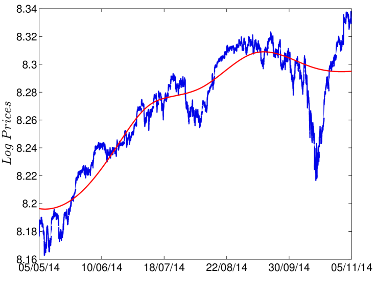
Figure 8: EMD analysis for the NASDAQ index. Captions for figures (a) and (b) are the same as captions for figures (4) and (6) respectively.

The variance scaling properties of the BOVESPA index (Brazil) are presented in Figure 9. For this stock index, the EMD identifies long period cycles with larger variance than what would be expected from Bm, see Figure 9. However, the linear fit between the logarithmic value of IMF variances and periods is in general good with $R^{2}=0.989$. The goodness of the linear fit between the Bm simulations is $\left<R_{Bm}^{2}\right>=0.977$, placing this index at the second position. Such a good ranking for this market may be unexpected, but we must stress that it only reflects the six-month period of observations. From Figure 9, we can see that this was a rather random but calm period.

Figure 9: EMD analysis for the BOVESPA index. Captions for figures (a) and (b) are the same as captions for figures (4) and (6) respectively.

For the NIKKEI 225 index (Japan), we obtained 22 IMFs and a residue. Similar as the NASDAQ index, the number of components is considerable larger than what would be expected from Bm, i.e., $\log_{2}(75600)$=16.2. These many oscillations, specially the high frequency components, generate a non-linear behaviour that deviates from Bm. Given the anomalous scaling behaviour of this stock index, see Figure 10, we obtained $\left<R_{Bm}^{2}\right>=0.949$, ranking it at the $16^{th}$ position.

Figure 10: EMD analysis for the NIKKEI 225 index. Captions for figures (a) and (b) are the same as captions for figures (4) and (6) respectively.

Finally, the DSM stock index (Qatar) is displayed in Figure 11. The log-price time series and its respective ‘trend’ are displayed in Figure 11. In Figure 11, we observe the poor liner fit of Equation 6 that is characterized by a considerable steep slope. We obtained $R^{2}=0.971$, ranking this index at the lowest position. Furthermore, if we compare its IMF variances against the Bm linear fits, we observe that most of the variance values (red diamonds) follow outside the band expected from Bm. The large variance of the low frequency components suggests the presence of important long period cycles. Given its deviations from Bm behaviour, this index is also ranked the lowest with respect to the measure $\left<R_{Bm}^{2}\right>=0.928$.

Figure 11: EMD analysis for the DSM index. Captions for figures (a) and (b) are the same as captions for figures (4) and (6) respectively.

5 Conclusions

We explored the scaling properties of EMD, an algorithm that detrends and separates time series into a set of oscillating components called IMFs which are associated with specific time-scales. We empirically showed that fBm obeys a scaling law that relates linearly the logarithm of the variance and the logarithm of the period of the IMFs. For fBm, we demonstrated that the extracted coefficient of proportionality equals the scaling exponent $H$ multiplied by two. When applied to stock market indices, the EMD reveals instead different scaling laws that can deviate significantly from both Brownian motion and fractional Brownian motion behaviour. In particular, we noted that the EMD of high frequency financial data results in a larger number of IMFs than what would be expected from Brownian motion. These many components, specially with high frequencies, create a curvature that disobeys the linearity in the log-log relation between IMF variance and period found in fBm. This is a direct indication of anomalous scaling that reveals a more complex structure in financial data than in self-similar processes.

In this study, we applied EMD to 22 different stock indices and observed that developed markets (European and North American markets) tend to have scaling properties closer to Brownian motion properties. Conversely, larger deviations from uni-scaling laws are observed in some emerging markets such as Malaysian and Qatari.

These findings are in agreement with the discernible characteristics of developed and emerging markets, the former type being more likely to exhibit an efficient behaviour, see for example [18, 42]. Compared to previous approaches, the EMD method has the advantage to directly quantify the cyclical components with strong deviations, giving a further instrument to understand the origin of market inefficiencies.

References

- [1] M. M. Dacorogna, R. Gençay, U. Müller, R. B. Olsen, O. V. Pictet, An introduction to high frequency finance, Academic Press, San Diego, 2001.
- [2] M. Bartolozzi, C. Mellen, T. Di Matteo, T. Aste, Multi-scale correlations in different futures markets, The European Physical Journal B 58 (2) (2007) 207–220.
- [3] B. Mandelbrot, The Variation of Certain Speculative Prices, The Journal of Business 36 (1963) 394.
- [4] B. Mandelbrot, H. M. Taylor, On the distribution of stock price differences, Operations Research 15 (6) (1967) 1057–1062.
- [5] U. A. Muller, M. M. Dacorogna, R. B. Olsen, O. V. Pictet, M. Schwarz, C. Morgenegg, Statistical study of foreign exchange rates, empirical evidence of a price change scaling law, and intraday analysis, Journal of Banking & Finance 14 (6) (1990) 1189–1208.
- [6] R. Gençay, F. Selçuk, B. Whitcher, Scaling properties of foreign exchange volatility, Physica A: Statistical Mechanics and its Applications 289 (1-2) (2001) 249 – 266.
- [7] R. Cont, Empirical properties of asset returns: stylized facts and statistical issues, Quantitative Finance 1 (2001) 223–236.
- [8] F. Lillo, J. D. Farmer, The long memory of the efficient market, Studies in Nonlinear Dynamics & Econometrics 8 (3) (2004) 1–35.
- [9] J. B. Glattfelder, A. Dupuis, R. B. Olsen, Patterns in high-frequency fx data: discovery of 12 empirical scaling laws, Quantitative Finance 11 (4) (2011) 599–614.
- [10] E. F. Fama, The behavior of stock-market prices, The Journal of Business 38 (1) (1965) 34–105.
- [11] H. E. Hurst, Long-term storage capacity of reservoirs, Trans. Amer. Soc. Civil Eng. 116 (1951) 770–808.
- [12] E. E. Peters, Fractal Market Analysis: Applying Chaos Theory to Investment and Economics, Wiley, New York, 1994.
- [13] B. LeBaron, Agent-based Computational Finance, in: L. Tesfatsion, K. L. Judd (Eds.), Handbook of Computational Economics, Vol. 2 of Handbook of Computational Economics, Elsevier, 2006, Ch. 24, pp. 1187–1233.
- [14] H. P. Boswijk, C. Hommes, S. Manzan, Behavioral heterogeneity in stock prices, Journal of Economic Dynamics and Control 31 (6) (2007) 1938–1970.
- [15] C. Chiarella, R. Dieci, X.-Z. He, Heterogeneity, Market Mechanisms, and Asset Price Dynamics, Handbook of Financial Markets: Dynamics and Evolution, Elsevier, 2009, p. 277–344.
- [16] T. Lux, Stochastic Behavioral Asset Pricing Models and the Stylized Facts, Handbook of Financial Markets: Dynamics and Evolution, Elsevier, 2009, pp. 161–215Hens, T. and K.R. SchenkHoppe.
- [17] W. Feller, An introduction to probability theory and its applications. Vol. II, 2nd Edition, John Wiley & Sons Inc., New York, 1966.
- [18] T. Di Matteo, T. Aste, M. Dacorogna, Scaling behaviors in differently developed markets, Physica A: Statistical Mechanics and its Applications 324 (1) (2003) 183–188.
- [19] T. Di Matteo, Multi-scaling in finance, Quantitative Finance 7 (1) (2007) 21–36.
- [20] A. Chakraborti, I. M. Toke, M. Patriarca, F. Abergel, Econophysics review: I. Empirical facts, Quantitative Finance 11 (7) (2011) 991–1012.
- [21] J. Barunik, T. Aste, T. Di Matteo, R. Liu, Understanding the source of multifractality in financial markets, Physica A: Statistical Mechanics and its Applications 391 (17) (2012) 4234 – 4251.
- [22] T. D. M. R. J. Buonocore, T. Aste, Measuring multiscaling in financial time-series, submitted (2015).
- [23] R. N. Mantegna, H. E. Stanley, Scaling behaviour in the dynamics of an economic index, Nature 376 (6535) (1995) 46–49.
- [24] R. N. Mantegna, H. E. Stanley, An introduction to econophysics: correlations and complexity in finance, Cambridge University press, Cambridge, 2000.
- [25] N. E. Huang, Z. Shen, S. R. Long, M. C. Wu, H. H. Shih, Q. Zheng, N.-C. Yen, C. C. Tung, H. H. Liu, The empirical mode decomposition and the Hilbert spectrum for nonlinear and non-stationary time series analysis, Proceedings of the Royal Society of London. Series A: Mathematical, Physical and Engineering Sciences 454 (1971) (1998) 903–995.
- [26] N. E. Huang, M.-L. Wu, W. Qu, S. R. Long, S. S. P. Shen, Applications of Hilbert-Huang transform to non-stationary financial time series analysis, Appl. Stochastic Models Bus. Ind. 19 (3) (2003) 245–268.
- [27] M.-C. Wu, Phase correlation of foreign exchange time series, Physica A: Statistical Mechanics and its Applications 375 (2) (2007) 633 – 642.
- [28] K. Guhathakurta, I. Mukherjee, A. R. Chowdhury, Empirical mode decomposition analysis of two different financial time series and their comparison, Chaos, Solitons & Fractals 37 (4) (2008) 1214 – 1227.
- [29] X.-Y. Qian, G.-F. Gu, W.-X. Zhou, Modified detrended fluctuation analysis based on empirical mode decomposition for the characterization of anti-persistent processes, Physica A: Statistical Mechanics and its Applications 390 (23) (2011) 4388–4395.
- [30] N. Nava, T. Di Matteo, T. Aste, Time-dependent scaling patterns in high frequency financial data, submitted (2015).
- [31] Y. Huang, F. G. Schmitt, Z. Lu, Y. Liu, Analysis of daily river flow fluctuations using empirical mode decomposition and arbitrary order Hilbert spectral analysis, Journal of Hydrology 373 (1–2) (2009) 103 – 111.
- [32] Z. Guo, W. Zhao, H. Lu, J. Wang, Multi-step forecasting for wind speed using a modified emd-based artificial neural network model, Renewable Energy 37 (1) (2012) 241 – 249.
- [33] R. Balocchi, D. Menicucci, E. Santarcangelo, L. Sebastiani, A. Gemignani, B. Ghelarducci, M. Varanini, Deriving the respiratory sinus arrhythmia from the heartbeat time series using empirical mode decomposition, Chaos, Solitons & Fractals 20 (1) (2004) 171 – 177.
- [34] Z. Peng, P. W. Tse, F. Chu, A comparison study of improved Hilbert–-Huang transform and wavelet transform: Application to fault diagnosis for rolling bearing, Mechanical Systems and Signal Processing 19 (5) (2005) 974 – 988.
- [35] P. Flandrin, G. Rilling, P. Goncalves, Empirical mode decomposition as a filter bank, Signal Processing Letters, IEEE 11 (2) (2004) 112–114.
- [36] B. B. Mandelbrot, The fractal geometry of nature, Freeman, 1982.
- [37] B. Mandelbrot, A. Fisher, L. Calvet, A Multifractal Model of Asset Returns, Cowles Foundation Discussion Papers 1164, Cowles Foundation for Research in Economics, Yale University (1997).
- [38] L. Calvet, A. Fisher, Multifractality in asset returns: Theory and evidence, The Review of Economics and Statistics 84 (3) (2002) 381–406.
- [39] B. B. Mandelbrot, J. W. V. Ness, Fractional Brownian Motions, Fractional Noises and Applications, SIAM Review 10 (4) (1968) pp. 422–437.
- [40] P. Flandrin, P. Gonçalves, Empirical mode decompositions as data-driven wavelet-like expansions, Int. J. of Wavelets, Multiresolution and Information Processing 2 (4) (2004) 477–496.
- [41] C. R. Rao, Linear statistical inference and its applications, Wiley, 1973.
- [42] T. Di Matteo, T. Aste, M. Dacorogna, Long-term memories of developed and emerging markets: Using the scaling analysis to characterize their stage of development, Journal of Banking & Finance 29 (4) (2005) 827 – 851.