Abstract: Motivated by applications in telecommunications, computer science and physics, we consider a discrete-time Markov process with restart. At each step the process either with a positive probability restarts from a given distribution, or with the complementary probability continues according to a Markov transition kernel. The main contribution of the present work is that we obtain an explicit expression for the expectation of the hitting time (to a given target set) of the process with restart. The formula is convenient when considering the problem of optimization of the expected hitting time with respect to the restart probability. We illustrate our results with two examples in uncountable and countable state spaces and with an application to network centrality.

Key-words: Discrete-time Markov Process with Restart, Expected Hitting Time, Network Centrality

Le Temps de Premier Passage dans les Processus de Markov avec Redémarrage et leur Application à la Mesure de Centralité de Réseau

Résumé : Motivé par diverses applications provenant de télécommunications, informatique et de la physique, nous considerons un processus generale de Markov dans l’espace de Borel avec une possibilité de redémarrage. À chaque étape, avec une probabilité le processus redémarre a partir d’une distribution donnée et avec la probabilité complémentaire le processus continue l’évolution selon une noyau de Markov. Nous étudions l’espérance du temps de premier passage à l’ensemble donné. Nous obtenons une formule explicite pour l’espérance du temps de premier passage et démontrons que le processus avec redémarrage est Harris positif récurrent. Ensuite, nous établissons que les assertions suivantes sont équivalentes : (a) le fait d’être limité (par rapport à l’état initiale) de l’espérance du temps de premier passage; (b) la finitude de l’espérance du temps de premier passage pour presque tous les états initiaux par rapport à la probabilité invariante unique; et, (c) l’ensemble cible est de mesure positive par rapport à la probabilité invariante. Enfin, nous illustrons nos résultats théoriques avec deux exemples dans les espaces dénombrables et non dénombrables et avec l’application à la mesure de centralité de réseau.

Mots-clés : Processus de Markov en Temps Discret, L’Espérance du Temps de Premier Passage, La Mesure de Centralité de Réseau

1 Introduction

We give a self-contained study of a discrete-time Markov process with restart. At each step the process either with the positive probability $p$ restarts from a given distribution, or with the complementary probability $1-p$ continues according to a Markov transition kernel. Such processes have many applications in telecommunications, computer science and physics. Let us cite just a few. Both TCP (Transmission Control Protocol) and HTTP (Hypertext Transfer Protocol) can be viewed as protocols restarting from time to time, [16], [20]. The PageRank network centrality [10], in information retrieval, models the behaviour of an Internet user surfing the web and restarting from a new topic from time to time. The sybil attack resistant network centralities based on the hitting times of a random walk with restart have been proposed in [14, 18]. Markov processes with restart are useful for the analysis of replace and restart types protocols in computer reliability, [2], [3], [17]. The restart policy is also used to speedup the Las Vegas type randomized algorithms [1], [19]. Finally, human and animal mobility patterns can be modeled by Markov processes that restart from some locations [12], [24].

The main focus of the present work is the expectation of the hitting time (to a given target set) of the process with restart, for which we obtain simple explicit expressions in terms of the expected discounted hitting time of the original process without restart; see Theorem 2.1. These formula is useful in the optimization of the expected hitting time with respect to the restart probability. In addition, the formulae allow us to either refine, or give simple and self-contained proofs of the stability results for the process with restart in terms of hitting times. Finally, in Section 3, we illustrate the main results with two examples in uncountable and countable state spaces and with an application to network centrality. In particular, we show that the hitting time based network centrality can be more discerning than PageRank.

Let us mention some related work to the present one in the current literature. The continuous-time Markov process with restart was considered in [7]. According to Theorem 2.2 in [7], the continuous-time Markov process with restart is positive Harris recurrent in case the original process is honest. At the same time, the process with restart is not positive Harris recurrent if the original process is not honest (i.e., the transition kernel is substochastic; in case the state space is countable, that means the accumulation of jumps). The objective of [7] does not lie in the expected hitting time, but in the representation of the transition probability function of the (continuous-time) process with restart in terms of the one of the original (continuous-time) process without restart. This is trivial in the present discrete-time setup. Here our focus is on the characterization of the expected hitting time. We also would like to mention the two works [11] and [15], dealing with the control theoretic formulation, where the controller decides (dynamically) whether it is beneficial or not to perform a restart at the current state. That line of research can be considered complementary to ours.

The rest of this paper is organized as follows. The description of the process with restart and the main statements are presented in Section 2, which are illustrated by two examples and network centrality application in Section 3. The paper is finished with a conclusion in Section 4.

2 Main statements

Let us introduce the model formally. As in [21], let $E$ be a nonempty locally compact Borel state space endowed with its Borel $\sigma$-algebra ${\cal B}(E).$ Consider a discrete-time Markov chain $\tilde{X}=\{\tilde{X}_{t},~{}t=0,1,\dots\}$ in the state space $E$ with the transition probability function $\tilde{P}(x,dy)$ being defined by

$$\tilde{P}(x,\Gamma):=p\nu(\Gamma)+(1-p)P(x,\Gamma),$$ (1)

for each $\Gamma\in{\cal B}(E)$, where $p\in(0,1)$ and $P(x,dy)$ is a transition probability function, and $\nu$ is a probability measure on ${\cal B}(E).$ Let $X:=\{X_{t},t=0,1,\dots\}$ denote the Markov chain corresponding to the transition probability $P(x,dy)$. We assume the two processes $X$ and $\tilde{X}$ are defined on the common probability space $(\Omega,\cal F,\mathbb{P})$; if we emphasize that the initial state is $x\in E,$ then $E_{x}$ denotes the corresponding expectation operator, and the notation $P_{x}$ is similarly understood.

The process $\tilde{X}$ is understood as the modified version of the process $X$, and is obtained by restarting (independently of anything else) the process $X$ after each transition with probability $p\in(0,1)$ and the distribution of the state after each restart being given by $\nu;$ whereas if there is no restart after the transition (with probability $1-p$), the distribution of the post-transition state is $P(x,dy)$ (given that the current state is $x$).

The following notation is used throughout this paper. Let $P^{t}(x,dy),~{}t=0,1,\dots,$ be defined iteratively as follows; for each $\Gamma\in{\cal B}(E),$

$$P^{0}(x,\Gamma) := I\{x\in\Gamma\},$$

$$P^{t+1}(x,\Gamma) := \int_{E}P^{t}(x,dy)P(y,\Gamma).$$

The power of other kernels is understood similarly.

Finally, thoughout this paper, the convention $0\cdot+\infty:=0$ is in use.

2.1 Known facts

The materials in this subsection are standard and known from [21]. The purpose here is to give a short and self-contained presentation. The main result of this paper is postponed to the next subsection.

From (1) it is clear that the process $\tilde{X}$ is Harris recurrent with an irreducibility measure $\nu$. (Recall that the process $\tilde{X}$ is $\nu$-irreducible if for each set $\Gamma\in{\cal B}(E)$ satisfying $\nu(\Gamma)>0$, it holds that $P_{x}(\tau_{\Gamma}<\infty)>0$ for each $x\in E,$ where

$$\tau_{\Gamma}:=\inf\{t=1,2,\dots:\tilde{X}_{t}\in\Gamma\}.$$ (2)

As usual, $\inf\emptyset:=\infty.$) If a Harris recurrent process admits an invariant probability, then it is called positive Harris recurrent; in that case the invariant probability is unique. We verify that $\tilde{X}$ is positive Harris recurrent with the unique invariant probability $q$ given in the next statement.

Proposition 2.1

The process $\tilde{X}$ is positive Harris recurrent with the unique invariant probability measure $q(dy)$ given by

$$q(\Gamma)=\int_{E}\sum_{t=0}^{\infty}p(1-p)^{t}P^{t}(y,\Gamma)\nu(dy)$$ (3)

for each $\Gamma\in{\cal B}(E).$

Proof. Clearly, $q(dy)$ is a probability measure, and routine calculations verify

$$q(\Gamma)=\int_{E}q(dx)\tilde{P}(x,\Gamma)$$

for each $\Gamma\in{\cal B}(E)$. $\hfill\Box$

We strengthen the above statement in the next corollary. Observe that the process $\tilde{X}$ is aperiodic in the sense of p.118 of [21], and the state space $E$ is a petite set since $\tilde{P}(x,\cdot)\geq p\nu(\cdot)$ for each $x\in E$. By Theorem 16.0.2 (vi) of [21], we see that the process $\tilde{X}$ is uniformly ergodic (see also related arguments in [22, 23]). However, in the next statement, we give a direct simple proof of this fact, and obtain the rate of convergence in terms of the restart probability. Below, $||\cdot||_{TV}$ stands for the total variation norm of finite signed measures.

Corollary 2.1

The process $\tilde{X}$ is uniformly ergodic with the unique invariant probability measure $q(\cdot)$ given in Proposition 2.1. In particular, we have

$$||\tilde{P}^{n}(x,\cdot)-q(\cdot)||_{TV}\leq 2(1-p)^{n}.$$ (4)

Proof. We first note that

$$\tilde{P}^{n}(x,\Gamma)=\int_{E}\sum_{t=0}^{n-1}p(1-p)^{t}P^{t}(y,\Gamma)\nu(dy)+(1-p)^{n}P^{n}(x,\Gamma),$$

which can be easily shown by induction. Next, using the above expression and Proposition 2.1, we can write

$$||\tilde{P}^{n}(x,\cdot)-q(\cdot)||_{TV}=||-\int_{E}\sum_{t=n}^{\infty}p(1-p)^{t}P^{t}(y,\cdot)\nu(dy)+(1-p)^{n}P^{n}(x,\cdot)||_{TV}$$

$$\leq (1-p)^{n}||-\int_{E}\sum_{t=0}^{\infty}p(1-p)^{t}P^{t+n}(y,\cdot)\nu(dy)+P^{n}(x,\cdot)||_{TV}$$

$$\leq 2(1-p)^{n}.$$

Thus, we have established inequality (4) and hence the uniform ergodicity. $\hfill\Box$

2.2 Hitting times

In this paper we are primarily interested in the expected hitting time of the process $\tilde{X}$ to a given set $H\in{\cal B}(E),$ defined by

$$\eta_{H}:=\inf\{t=0,1,\dots:\tilde{X}_{t}\in H\}.$$

For the future reference, we put

$${}_{H}P^{0}(x,E):=I\{x\in E\setminus H\}.$$

Denote

$$V(x):=E_{x}\left[\eta_{H}\right]$$ (5)

and let

$${}_{H}P(x,\Gamma)=P(x,\Gamma\setminus H)$$

be the taboo transition kernel with respect to the set $H$. Then, one can write

$$V(x)=1+p\int_{E}V(y)\nu(dy)+(1-p)\int_{E}V(y){}_{H}P(x,dy),\quad\forall~{}x\in E\setminus H,$$

$$V(x)=0,\quad\forall~{}x\in H.$$ (6)

Furthermore, it is well known that the function $V(x)$ defined by (5) is the minimal nonnegative (measurable) solution to equation (2.2), and can be obtained by iterations

$$V^{(n+1)}(x)=1+p\int_{E}V^{(n)}(y)\nu(dy)+(1-p)\int_{E}V^{(n)}(y){}_{H}P(x,dy),~{}x\in E\setminus H,\quad n=0,1,...$$

with $V^{(n)}(x)=0$ if $x\in H$ for each $n=0,1,\dots$, and $V^{(0)}(x)\equiv 0$; c.f. e.g., Proposition 9.10 of [9].

One can actually obtain the minimal nonnegative solution to (2.2) in the explicit form.

Theorem 2.1

(a) The minimal nonnegative solution to (2.2) is given by the following explicit form

$$V(x)=V_{1}(x)\sum_{t=0}^{\infty}\left(p\int_{E}V_{1}(y)\nu(dy)\right)^{t},\quad\forall~{}x\in E\setminus H,$$

$$V(x)=0,\quad\forall~{}x\in H,$$ (7)

where the function $V_{1}$ is given by

$$V_{1}(x):=\sum_{t=0}^{\infty}(1-p)^{t}{}_{H}P^{t}(x,E),\quad\forall~{}x\in E\setminus H;$$

$$V_{1}(x):=0,\quad\forall~{}x\in H.$$ (8)

It coincides with the unique bounded solution to the equation

$$V_{1}(x)=1+(1-p)\int_{E}V_{1}(y){}_{H}P(x,dy),\quad\forall~{}x\in E\setminus H;$$

$$V_{1}(x)=0,\quad\forall~{}x\in H.$$ (9)

(b) If $q(H)>0,$ then

$$V(x)=\frac{V_{1}(x)}{1-p\int_{E}V_{1}(y)\nu(dy)}<\infty,\quad\forall~{}x\in E\setminus H,$$

$$V(x)=0,\quad\forall~{}x\in H.$$ (10)

Proof. (a) Observe that the function $V_{1}$ given by (2.1) represents the expected total discounted time before the first hitting of the process $X$ at the set $H$ given the initial state $x$ and the discount factor $1-p.$ It thus follows from the standard result about the discounted dynamic programming with a bounded reward that the function $V_{1}$ is the unique bounded solution to equation (2.1); see e.g., Theorem 8.3.6 of [13].

Now by multiplying both sides of the equation (2.1) by the expression

$$\sum_{t=0}^{\infty}\left(p\int_{E}V_{1}(y)\nu(dy)\right)^{t}$$

for all $x\in E\setminus H,$ it can be directly verified that the function $V$ defined in terms of $V_{1}$ by (2.1) is a nonnegative solution to (2.2). We show that it is indeed the minimal nonnegative solution to (2.2) as follows.

Let $U\geq 0$ be an arbitrarily fixed nonnegative solution to (2.2). It will be shown by induction that

$$U(x)\geq V_{1}(x)\sum_{t=0}^{n}\left(p\int_{E}V_{1}(y)\nu(dy)\right)^{t}~{}\forall~{}n=0,1,\dots,~{}\forall~{}x\in E.$$ (11)

The case when $x\in H$ is trivial.

Let $x\in E\setminus H$ be arbitrarily fixed. It follows from (2.2) that

$$U(x)\geq 1+(1-p)\int_{E}{}_{H}P(x,dy)=\sum_{t=0}^{1}(1-p)^{t}\left(\int_{E}{}_{H}P^{t}(x,dy)\right)\geq 1.$$ (12)

If for some $n\geq 1$

$$U(x)\geq\sum_{t=0}^{n}(1-p)^{t}\left(\int_{E}{}_{H}P^{t}(x,dy)\right),$$ (13)

then by (2.2),

$$U(x) \geq 1+(1-p)\int_{E}U(y){}_{H}P(x,dy)$$

$$\geq 1+(1-p)\int_{E}\left(\sum_{t=0}^{n}(1-p)^{t}\left(\int_{E}{}_{H}P^{t}(y,dz)\right)\right){}_{H}P(x,dy)$$

$$= \sum_{t=0}^{n+1}(1-p)^{t}\left(\int_{E}{}_{H}P^{t}(x,dy)\right),$$

and so (13) holds for all $n\geq 0$ and thus by (2.1)

$$U(x)\geq V_{1}(x).$$

Consequently, (11) holds when $n=0.$

Suppose (11) holds for $n$, and consider the case of $n+1.$ Then from (2.2),

$$U(x) = 1+p\int_{E}U(y)\nu(dy)+(1-p)\int_{E}U(y){}_{H}P(x,dy)$$ (14)

$$\geq \sum_{t=0}^{n+1}\left(p\int_{E}V_{1}(y)\nu(dy)\right)^{t}+(1-p)\int_{E}U(y){}_{H}P(x,dy),$$

where the inequality follows from the inductive supposition. Define the function $W$ on $E$ by

$$W(z)=\frac{U(z)}{\sum_{t=0}^{n+1}\left(p\int_{E}V_{1}(y)\nu(dy)\right)^{t}},\quad\forall~{}z\in E.$$

Then by (14),

$$W(x)\geq 1+(1-p)\int_{E}{}_{H}P(x,dy)=\sum_{t=0}^{1}(1-p)^{t}\left(\int_{E}{}_{H}P^{t}(x,dy)\right);$$

c.f. (12). Now, based on (14), a similar reasoning by induction as to the verification of (13) for all $n\geq 0$ shows that

$$W(x)\geq\sum_{t=0}^{k}(1-p)^{t}\left(\int_{E}{}_{H}P^{t}(x,dy)\right),\quad\forall~{}k=0,1,\dots,$$

and thus $W(x)\geq V_{1}(x)$. This means

$$U(x)\geq V_{1}(x)\sum_{t=0}^{n+1}\left(p\int_{E}V_{1}(y)\nu(dy)\right)^{t}.$$

Thus by induction, (11) holds for all $n\geq 0$, and thus

$$U(x)\geq V(x)$$

by (2.1), as desired.

(b) If $q(H)>0$, then there exists some $T\geq 0$ such that $\int_{E}P^{T}(y,H)\nu(dy)>0$, meaning that there exists some $T^{\prime}\leq T$ such that $\int_{E}{}_{H}P^{T^{\prime}}(x,E)\nu(dx)<1$. Thus,

$$0\leq p\int_{E}\sum_{t=0}^{\infty}(1-p)^{t}{}_{H}P^{t}(y,E)\nu(dy)<1,$$

and so the geometric series $\sum_{t=0}^{\infty}\left(p\int_{E}V_{1}(y)\nu(dy)\right)^{t}$ converges. The statement follows. $\hfill\Box$

The next corollary is immediate.

Corollary 2.2

If $q(H)>0$, then both $V_{1}(x)$ and $V(x)$ are bounded with respect to the state $x\in E$. In particular, we have

$$V_{1}(x)\leq\frac{1}{p}.$$

There is a nice probabilistic interpretation of the decomposition presented in Theorem 2.1. Suppose $q(H)>0,$ which is case (b) in Theorem 2.1. Let us make a change of variable

$$\rho(x)=1-pV_{1}(x)=1-p\sum_{t=0}^{\infty}(1-p)^{t}{}_{H}P^{t}(x,E)=P_{x}[\mbox{hit before restart}].$$

Then, equation (2.1) takes the form

$$V(x)=\frac{1-\rho(x)}{p\int_{E}\rho(y)\nu(dy)}=\frac{P_{x}[\mbox{no hit before restart}]}{pP_{\nu}[\mbox{hit before restart}]}.$$

The expected number of steps in a cycle from one restart to another is $1/p$, and the expected number of cycles until we hit the set $H$ is roughly $1/P_{\nu}[\mbox{hit before restart}]$. Thus, the total expected steps is approximately equal to $1/(pP_{\nu}[\mbox{hit before restart}])$. This is only an approximation since we did not carefully take into account the impact of the first and the last incomplete cycles. It turns out that the factor $P_{x}[\mbox{no hit before restart}]$ gives the necessary correction. Theorem 2.1 can be viewed as a generalization of the results of [5, 14] to the general state space from the finite state space.

We also have the following chain of equivalent statements.

Theorem 2.2

The following statements are equivalent.

(a) $q(H)>0.$

(b) $V(x)=E_{x}[\eta_{H}]<\infty$ for each $x\in E.$

(c) $V(x)=E_{x}[\eta_{H}]<\infty$ for almost all $x\in E$ with respect to $q(dy).$

(d) $\sup_{x\in E}V(x)=\sup_{x\in E}E_{x}[\eta_{H}]<\infty$.

The proof of this theorem follows from the next lemma.

Lemma 2.1

Statements (a) and (c) in Theorem 2.2 are equivalent.

Proof. Statement (a) implies statement (c) by Theorem 2.1(b). It remains to show that statement (c) implies statement (a). To this end, suppose for contradiction that statement (a) does not hold, i.e., $q(H)=0.$ Then it follows from (3) that

$$\int_{E}\sum_{t=0}^{\infty}P^{t}(y,H)\nu(dy)=0.$$

Thus, there exists a measurable subset $\Gamma$ of $E\setminus H$ such that

$$\nu(\Gamma)=1$$ (15)

and

$$P_{x}[\eta_{H}^{X}=\infty]=1~{}\forall~{}x\in\Gamma,$$ (16)

where

$$\eta_{H}^{X}:=\inf\{t=0,1,\dots:X_{t}\in H\}.$$ (17)

Let $x\in\Gamma$ be fixed. Then by (2.1) and (16)

$$V_{1}(x)=E_{x}\left[\sum_{t=0}^{\eta^{X}_{H}-1}(1-p)^{t}\right]=E_{x}\left[\sum_{t=0}^{\infty}(1-p)^{t}\right]=\frac{1}{p}.$$

Since $x\in\Gamma$ is arbitrarily fixed, and $\nu(\Gamma)=1$ by (15), we see from (2.1) and the fact that $V_{1}(y)\geq 1$ if $y\in E\setminus H$ that $V(y)=\infty$ for each $y\in E\setminus H$. Since $q(E\setminus H)=1,$ we see that statement (c) does not hold. $\hfill\Box$

Proof of Theorem 2.2. From Theorem 2.1(b), we see that (a) implies (b), which implies (c). From Lemma 2.1, (c) implies (a). Clearly, (d) implies (b). Finally, (a) implies (d) because $V_{1}(x)$ is bounded; see Corollary 2.2. $\hfill\Box$

Remark 2.1

Corollary 2.1 and Theorem 16.0.2 of [21] immediately give the relation $(a)\Rightarrow(d)\Rightarrow(b)\Rightarrow(c)$ in Theorem 2.2. However, we gave its self-contained proof in the above without referring to the result concerning the general Markov chains in [21].

2.3 Optimization problem

Next let us consider the dependance of $V(x)$ on the restart probability $p$ for each fixed $x\in E$. When we emphasize the dependance on $p$, we explicitly write $V(x,p)$ and $V_{1}(x,p).$ In the above, $p\in(0,1)$ was fixed. Now we formally put

$$V(x,0):=\sum_{t=0}^{\infty}{}_{H}P^{t}(x,E)\in[1,\infty],\forall~{}x\in E\setminus H;$$

$$V(x,0):=0,\forall~{}x\in H,$$

which represents the expected hitting time of the process without restart, and

$$V(x,1):=\frac{1}{\nu(H)}\in[1,\infty],\forall~{}x\in E\setminus H;$$

$$V(x,1):=0,\forall~{}x\in H,$$

which represents the expected hitting time of the process that restarts with full probability at each transition. Here and below, $\frac{c}{0}:=\infty$ for any $c>0.$ As usual, the continuity of $V(x,p)$ at $p=a$ means $\lim_{p\rightarrow a}V(x,p)=V(x,a)\in[-\infty,\infty].$

Theorem 2.3

Suppose

$$\int_{E}\sum_{t=0}^{\infty}P^{t}(y,H)\nu(dy)>0.$$ (18)

Then the function $V(x,p)$ is infinitely many times differentiable in $p\in(0,1)$ and is continuous in $p\in[0,1].$ As a consequence, the problem

Miniminize $$V(x,p) p\in[0,1]$$ with respect to (19)

is solvable.

Remark 2.2

The condition (18) in the above statement is equivalent to $q(H)>0$ for some and then all $p\in(0,1)$ by (3).

Proof of Theorem 2.3. If $x\in H,$ the statement holds trivially since $V(x,p)=0$ for each $p\in[0,1].$ Consider now $x\in E\setminus H.$ One can see that $V_{1}(x,p)$ (as given by (2.1)) and $(1-p\int_{E}V_{1}(y,p)\nu(dy))^{-1}$ are both infinitely many times differentiable in $p\in(0,1).$ It follows from this and (2.1) that $V(x,p)$ is infinitely many times differentiable in $p\in(0,1).$ For the the continuity of $V(x,p)$ at $p=0,$ it holds that

$$1-p\int_{E}V_{1}(y,p)\nu(dy)=1-p\int_{E}E_{y}\left[\sum_{t=0}^{\eta^{X}_{H}-1}(1-p)^{t}\right]\nu(dy)$$

$$=1-\int_{E}E_{y}\left[1-(1-p)^{\eta^{X}_{H}}\right]\nu(dy)=\int_{E}E_{y}\left[(1-p)^{\eta^{X}_{H}}\right]\nu(dy)\rightarrow 1,$$

as $p\rightarrow 0$, by the monotone convergence theorem; recall (17) for the definition of $\eta_{H}^{X}$. It follows from this fact, (2.1), (2.1) and the monotone convergence theorem that

$$\lim_{p\rightarrow 0}V(x,p) = \frac{\lim_{p\rightarrow 0}V_{1}(x,p)}{\lim_{p\rightarrow 0}\left\{1-p\int_{E}V_{1}(y,p)\nu(dy)\right\}}=V(x,0)$$

as desired. The continuity of the function $V(x,p)$ at $p=1$ can be similarly established. The last assertion is a well known fact; see e.g., [9]. $\hfill\Box$

We shall illustrate the optimization problem (19) by two examples in the next section.

3 Numerical examples and application

3.1 Uni-directional random walk on the line

Let $E=\mathbb{R}$, $H=[a,b]$ with $a<b$ being two real numbers. The process $X$ only moves to the right, and the increments of each of the transitions are i.i.d. exponential random variables with the common mean $\frac{1}{\mu}>0$. The restart probability is denoted as $p\in(0,1)$ as usual, and the restart distribution $\nu$ is arbitrary. Below by using Theorem 2.1 we provide the explicit formula for the expected hitting time at $H$ of the restarted process $\tilde{X}$. (Clearly, if the initial state is outside $H$, then the expected hitting time of the process $X$ at the set $H$ is infinite.)

We can give the following informal description of this example. There is a treasure hidden in the interval $[a,b]$ and one tries to find the treasure. Once the searcher checks one point in the interval $[a,b]$, he finds the treasure. The searcher has the means only to stop and to check points between the exponentially distributed steps. This models the cost of checking frequently. It is also natural to restart the search from some base. Intuitively, by restarting too frequently, the searcher spends most of the time near the base and does not explore the area sufficiently. On the other hand, restarting too seldom leads the search to very far locations where the searcher spends most of the time for nothing. Hence, intuitively there should be an optimal value for restarting probability.

One can verify that in this example the unique bounded solution to (2.1) is given by $V_{1}(x)=0$ for each $x\in[a,b]$,

$$V_{1}(x)=\frac{1}{p}$$ (20)

for each $x>b$,

$$V_{1}(x)=\frac{1}{p}-\frac{1-p}{p}\left(1-e^{-\mu(b-a)}\right)e^{-\mu(a-x)p}$$ (21)

for each $x<a.$ In fact, this can be conveniently established using the following probabilistic argument. Recall that $V_{1}(x)$ represents the expected total discounted time up to the hitting of the set $H$ by the process $X$; see (2.1). So for (20) one merely notes that with the initial state $x>b,$ $\eta^{X}_{H}=\infty$, where $\eta^{X}_{H}$ is defined by (17). For (21), one can write for each $x<a$ that

$$V_{1}(x) = E_{x}\left[\sum_{t=0}^{\eta^{X}_{H}-1}(1-p)^{t}\right]=\left.E_{x}\left[E_{x}\left[\sum_{t=0}^{\eta^{X}_{H}-1}(1-p)^{t}\right|\eta_{H}^{X}\right]\right].$$

Now the expected hitting time of the restarted process $\tilde{X}$ to the set $H=[a,b]$ is given by

$$V(x)=\left(\frac{1}{p}-\frac{1-p}{p}\left(1-e^{-\mu(b-a)}\right)e^{-\mu(a-x)p}\right)\sum_{t=0}^{\infty}\left(p\int_{E}V_{1}(y)\nu(dy)\right)^{t},$$

with the initial state $x<a$, and by

$$V(x)=\frac{1}{p}\sum_{t=0}^{\infty}\left(p\int_{E}V_{1}(y)\nu(dy)\right)^{t},$$

with the initial state $x>b$, recall (2.1). If the restart distribution $\nu$ is not concentrated on $(b,\infty)$, then $q(H)>0$, and by Theorem 2.1(b) we have

$$V(x)=\frac{\frac{1}{p}-\frac{1-p}{p}\left(1-e^{-\mu(b-a)}\right)e^{-\mu(a-x)p}}{1-p\int_{E}V_{1}(y)\nu(dy)},$$

with the initial state $x<a$ and by

$$V(x)=\frac{1}{p\left(1-p\int_{E}V_{1}(y)\nu(dy)\right)},$$

for each $x>b$. In particular, if the process restarts from a single point $r<a$, the above expressions can be specified to

$$V(x)=\frac{1-(1-p)(1-e^{-\mu(b-a)})e^{-\mu(a-x)p}}{p(1-p)(1-e^{-\mu(b-a)})e^{-\mu(a-r)p}},$$

for the initial state $x<a$ and to

$$V(x)=\left(\frac{1}{1-e^{-\mu(b-a)}}\right)\left(\frac{1}{p(1-p)e^{-\mu(a-r)p}}\right),$$

for each $x>b$. For the latter case ($x>b$), by standard analysis of derivatives, one can find the optimal value of the restart probability minimizing the expected hitting time of the process with restart in a closed form, as given by

$$p_{opt}=\frac{2}{2+\mu(a-r)+\sqrt{4+\mu^{2}(a-r)^{2}}}.$$

Now we can make several observations: the first somewhat interesting observation is that in the case when the initial state is to the right of the interval $[a,b]$, the value of the optimal restart probability does not depend on the length of the interval but only on the average step size and on the restart position. The second observation is that when $\mu(a-r)$ is small, i.e., when either the average step size is large or the restart position is close to $H$, the optimal restart probability is close to 1/2. Thirdly, when $\mu(a-r)$ is large, the optimal restart probability is small and reads

$$p_{opt}=\frac{1}{1+\mu(a-r)}+\mbox{o}\left(\frac{1}{\mu(a-r)}\right).$$

3.2 Random walk on the one dimensional lattice

Let us consider a symmetric random walk on the one dimensional lattice which aims to hit $H=\{0\}$ with restart at some node $r$. Assume without loss of generality that the restart state $r$ is on the positive half-line, i.e., $r>0$.

From Theorem 2.1 we conclude that it is sufficient to solve the following equations

$$V_{1}(k)=1+\frac{1-p}{2}[V_{1}(k-1)+V_{1}(k+1)],\quad k\neq 0,$$

$$V_{1}(0)=0.$$

Following the standard approach for solution of difference equations, we obtain

$$V_{1}(k)=c\alpha_{1}^{k}+\frac{1}{p},$$

where $\alpha_{1}<1$ is the minimal solution to the characteristic equation

$$\alpha=\frac{1-p}{2}[1+\alpha^{2}],$$

and the constant $c=-\frac{1}{p}$ comes from the condition $V_{1}(0)=0$. Consequently,

$$V(k)=\frac{V_{1}(k)}{1-pV_{1}(r)}=\frac{1-\alpha_{1}^{k}}{p\alpha_{1}^{r}}.$$

An elegant analysis can be done for the limiting case when the initial position $k$ goes large, and hence we now minimize $\lim_{k\rightarrow\infty}V(k)=1/(p\alpha_{1}^{r})$, or equivalently, maximize $p\alpha_{1}^{r}$ with respect to $p\in(0,1).$ This leads to the following equation for the optimal restart probability

$$\frac{p}{\alpha_{1}}\frac{d\alpha_{1}}{dp}=-\frac{1}{r}.$$ (22)

Indeed, we note that

$$\lim_{p\to 0}\frac{p}{\alpha_{1}}\frac{d\alpha_{1}}{dp}=0,~{}\lim_{p\to 1}\frac{p}{\alpha_{1}}\frac{d\alpha_{1}}{dp}=-\infty,$$

and

$$\frac{d}{dp}\left(\frac{p}{\alpha_{1}}\frac{d\alpha_{1}}{dp}\right)=-\frac{1}{\sqrt{1-(1-p)^{2}}}\frac{1-(1-p^{2})(1-p)}{(1-p)^{2}(1-(1-p)^{2})}<0.$$

Thus, the left hand side of (22) is a monotone function decreasing from zero to minus infinity. Consequently, the unique solution of equation (22) is the global minimizer of $1/(p\alpha_{1}^{r})$. The equation (22) can be transformed to the polynomial equation

$$\frac{1}{r^{2}}(1-p)^{2}(2-p)=p$$

Consider the case of large $r$. This is a so-called case of singular perturbation, as the small parameter $1/r^{2}$ is in front of the largest degree term, [4], [8]. It is not difficult to see that for large values of $r$, the equation has one real root that can be expanded as

$$p_{opt}=\frac{c_{1}}{r^{2}}+\frac{c_{2}}{r^{4}}+...$$ (23)

and two complex roots that move to infinity as $r\to\infty$. By substituting the series (23) into the polynomial equation, we can identify the terms $c_{i},i=1,2,...$. Thus, we obtain

$$p_{opt}=\frac{2}{r^{2}}-\frac{10}{r^{4}}+\mbox{o}(r^{-4}).$$

3.3 Application to network centrality

One of the main tasks in network analysis is to determine which nodes are more “central” than the others. Node degree and PageRank [10] are examples of widely used centrality measures. We note that PageRank is a stationary distribution of the random walk with restart and in our setting it is just measure $q$. Both node degree and PageRank are prone to manipulation or so-called “sybil attack”. To mitigate this problem, the authors of [14, 18] proposed hitting time based centrality measures. Here we show that the hitting time based centrality can be more discerning. Let us first consider a simple 6-node network with weighted edges, see Figure 1. The weights are depicted near the edges.

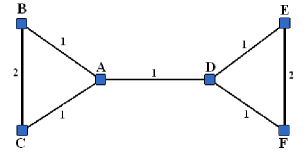
Figure 1: Example of 6-node network with weighted edges.

In Table 1 we give centrality values of the nodes with respect to node degree, PageRank and Expected Hitting Times starting and restarting both from the uniform distribution.

Table 1: Centralities for 6-node network.

Nodes	A	B	C	D	E	F
Node degree	3	3	3	3	3	3
PageRank, $\forall p$	1/6	1/6	1/6	1/6	1/6	1/6
Hitting time, $p=0.15$	6.28	8.28	8.28	6.28	8.28	8.28

The last row in Table 1 lists down the expected hitting times to the target state A, B, and so on. It is intuitively clear that nodes A and D are more central in this network. However, both node degree and PageRank indicate equal importance for the nodes. In contrast, the hitting time based centrality clearly indicates that nodes A and D are more central than the other nodes.

Let us now consider an example of a real social network. The example was taken from online social network VKontakte and represents a principal component of the interest group about Game Theory [6]. The example has 71 nodes and 116 weighted edges, see Figure 2 (taken from [6]). The edge weight is equal to the number of common friends. Only the edges with a weight more than two have been kept.

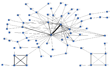
Figure 2: Example of a social network.

In Table 2 we provide top-10 lists of nodes according to node degree, PageRank and the expected hitting time.

Table 2: Top-10 lists for the social network example.

Node degree	1	8	4	20	6	56	7	28	44	32
PageRank, $p=0.15$	1	8	56	28	44	4	32	20	63	6
Hitting time, $p=0.15$	1	8	56	28	63	22	13	33	69	4

We observe that the top-10 list by PageRank has 9 nodes from the top-10 list by node degree. The top-10 list by the expected hitting time has only 5 nodes from the top-10 list by node degree. Note that nodes 22 and 13, which intuitively look quite central, are not in the top-10 list by PageRank.

Finally, we would like to show in Figure 3 the expected hitting time from node A to node B in the 6-node example as a function of the restart probability $p$. This function has a minimum inside the interval $[0,1]$. We think it will be interesting to study the minimization of the expected hitting time in the context of network community analysis.

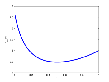
Figure 3: The expected hitting time from A to B.

4 Conclusion

In conclusion, in this paper we present a self-contained study of a discrete-time Markov process with restart. Our primary interest is in the expected hitting time of the process with restart to a target set. We obtained the formula of the expected hitting time of the restarted process to a target set, and considered the optimization problem of the expected hitting time with respect to the restart probability. We illustrated our results with two examples in uncountable and countable state spaces and one application to network centrality. In particular, we show that the network centrality based on hitting times is more selective. Our general results may also have potential application to network community analysis, which we intend to explore in the future.

References

- [1] Alt H., Guibas L., Mehlhorn K., Karp R. and Wigderson A., A method for obtaining randomized algorithms with small tail probabilities. Algorithmica. 16, 543-547, (1996).
- [2] Asmussen S., Fiorini P., Lipsky L., Rolski T. and Sheahan R., Asymptotic behavior of total times for jobs that must start over if a failure occurs. Mathematics of Operations Research. 33(4), 932-944, (2008).
- [3] Asmussen S., Lipsky L. and Thompson S., Checkpointing in failure recovery in computing and data transmission, In Proceedings of ASMTA’14, also in LNCS v.8499, 253-272, Springer, (2014).
- [4] Avrachenkov K., Filar J.A. and Howlett P.G., Analytic perturbation theory and its applications, SIAM, (2013).
- [5] Avrachenkov K. and Litvak N., The effect of new links on Google PageRank. Stochastic Models, 22(2), 319-331, (2006).
- [6] Avrachenkov K., Mazalov V. and Tsynguev B., Beta current flow centrality for weighted networks. In Proceedings of CSoNet 2015, also in Springer LNCS v.9197, 216-227, (2015).
- [7] Avrachenkov K., Piunovskiy A. and Zhang Y., Markov processes with restart. Journal of Applied Probability, 50, 960-968, (2013).
- [8] Baumgärtel H., Analytic perturbation theory for matrices and operators, Birkhäuser, Basel, (1985).
- [9] Bertsekas D. and Shreve S., Stochastic optimal control: the discrete-time case. Academic Press, New York, (1978).
- [10] Brin S. and Page L., The anatomy of a large-scale hypertextual Web search engine. Computer Networks and ISDN Systems, 30, 107-117, (1998).
- [11] Dumitriu I., Tetali P. and Winkler P., On playing golf with two balls. SIAM Journal on Discrete Mathematics. 16(4), 604-615, (2003).
- [12] González M.C., Hidalgo C.A. and Barabási A.-L., Understanding individual human mobility patterns. Nature, 453, 779-782, (2008).
- [13] Hernández-Lerma O. and Lasserre J.-B., Further topics in discrete-time Markov control processes. Springer, New York, (1999).
- [14] Hopcroft J. and Sheldon D., Manipulation-resistant reputations using hitting time. Internet Mathematics, 5(1-2), 71-90, (2008).
- [15] Janson S. and Peres Y., Hitting times for random walks with restarts. SIAM Journal on Discrete Mathematics. 26(2), 537-547, (2012).
- [16] Krishnamurthy B. and Rexford J., Web protocols and practice: HTTP/1.1, networking protocols, caching, and traffic measurement. Addison Wesley, (2001).
- [17] Kulkarni V., Nicola V. and Trivedi K., The completion time of a job on a multimode system. Advances in Applied Probability. 19, 932-954, (1987).
- [18] Liu B.K., Parkes D.C. and Seuken S., Personalized hitting time for informative trust mechanisms despite sybils. In Proceedings of the 2016 International Conference on Autonomous Agents & Multiagent Systems, pp. 1124-1132, (2016).
- [19] Luby M., Sinclair A. and Zuckerman D., Optimal speedup of Las Vegas algorithms. Information Processing Letters. 47, 173-180, (1993).
- [20] Maurer S.M. and Huberman B.A., Restart strategies and Internet congestion. Journal of Economic Dynamics and Control. 25, 641-654, (2001).
- [21] Meyn S. and Tweedie R., Markov chains and stochastic stability. Springer, London, (1993).
- [22] Nummelin E., MC’s for MCMC’ists. International Statistical Review. 70(2), 215-240, (2002).
- [23] Nummelin, E. and Tuominen, P., Geometric ergodicity of Harris recurrent Marcov chains with applications to renewal theory. Stochastic Processes and Their Applications. 12(2), pp.187-202, (1982).
- [24] Walsh P.D., Boyer D. and Crofoot M.C., Monkey and cell-phone-user mobilities scale similarly. Nature Physics. 6, 929-930, (2010).