Abstract: We consider a task of scheduling a crawler to retrieve content from several sites with ephemeral content. A user typically loses interest in ephemeral content, like news or posts at social network groups, after several days or hours. Thus, development of timely crawling policy for such ephemeral information sources is very important. We first formulate this problem as an optimal control problem with average reward. The reward can be measured in the number of clicks or relevant search requests. The problem in its initial formulation suffers from the curse of dimensionality and quickly becomes intractable even with moderate number of information sources. Fortunately, this problem admits a Whittle index, which leads to problem decomposition and to a very simple and efficient crawling policy. We derive the Whittle index and provide its theoretical justification.

Key-words: Whittle Index, Search Engine, Crawler, Ephemeral Content

Index de Whittle pour Crawling du Contenu Éphémère

Résumé : Nous considérons une tâche de la planification du parcours d’un robot pour récupérer le contenu éphémère de plusieurs sites web. Typiquement, un utilisateur de web perd intérêt pour le contenu éphémère, comme des nouvelles ou des posts aux réseaux sociaux, après plusieurs jours ou même heures. Donc, le développement de la planification dynamique du parcours de ces sources d’information éphémères est très important. Nous formulons d’abord ce problème comme un problème de commande optimale avec une récompense moyenne. La récompense peut être mesurée par le nombre de clics ou par le nombre de demandes de recherche pertinente. Le problème dans sa formulation initiale souffre de la “malédiction de la dimension” et devient rapidement inextricable même avec nombre modéré des sources d’information. Heureusement, ce problème admet un Index de Whittle, qui conduit à la décomposition du problème et à une politique de parcours très simple et efficace. Nous dérivons l’Index de Whittle et fournissons sa justification théorique.

Mots-clés : Index de Whittle, Moteur de Recherche, Crawler, Robot, Contenu Éphémère

1 Introduction

Nowadays an overwhelming majority of people find new information on the web at news sites, blogs, forums and social networking groups. Moreover, most information consumed is ephemeral in nature, that is, people tend to lose their interest in the content in several days or hours. The interest in a content can be measured in terms of clicks or number of relevant search requests. It has been demonstrated that the interest decreases exponentially over time [10, 15, 18].

In a series of works (see e.g., [7, 9, 8, 21] and references therein) the authors address the problem of refreshing documents in a database. However, these works do not consider the ephemeral nature of the information. Motivated by this challenge, the authors of [15] suggest a procedure for optimal crawling of ephemeral content. Specifically, the authors of [15] formulate an optimization problem for finding optimal frequencies of crawling for various information sources.

The approach presented in [15] is static, in the sense that the distribution of crawling effort among the content sources is always the same independent of the time epoch and, in particular, does not depend on any ‘state variable(s)’ evolving with time. With a dynamic policy, for instance, if there is not much new material on the principal information sources, the crawler could spend some time to crawl the sources with less popular content but which nevertheless bring noticeable rate of clicks or increase information diversity. Therefore, in the present work we suggest a dynamic formulation of the problem as an optimal control problem with average reward. The direct application of dynamic programming quickly becomes intractable even with moderate number of information sources, due to the so-called curse of dimensionality. Fortunately, the problem admits a Whittle index, which leads to problem decomposition and to a very simple and efficient crawling policy. We derive the Whittle index and provide its theoretical justification.

In [5, 16, 25] the authors study the interaction between the crawler and the indexing engine by means of optimization and control theoretic approaches. One of interesting future research directions is to take into account the indexing engine dynamics in the present context.

The general concept of the Whittle index was introduced by P. Whittle in [28]. This has been a very successful heuristic for restless bandits, which, while suboptimal in general, is provably optimal in an asymptotic sense [26, 27] and has good empirical performance. It and its variants have been used extensively in logistical and engineering applications, some recent instances of the latter in communications and control being for sensor scheduling [19], multi-UAV coordination [20], congestion control [3, 4, 13], channel allocation in wireless networks [14], cognitive radio [17] and real-time wireless multicast [23]. Book length treatments of indexable restless bandits appear in [12, 24].

2 Model

There are $N$ sources of ephemeral content. A content at source $i\in\{1,...,N\}$ is published with an initial utility modelled by a nonnegative random variable $\xi_{i}$ and decreasing exponentially over time with a deterministic rate $\mu_{i}$. The new content arrives at source $i\in\{1,...,N\}$ according to a time-homogeneous Poisson process with rate $\Lambda_{i}$. Thus, if source $i$’s content is crawled $\tau$ time units after its creation, its utility is given by $\xi_{i}\exp(-\mu_{i}\tau)$. The base utility $\xi_{i}$ is assumed independent identically distributed across contents at a given source, with a finite mean $\bar{\xi}_{i}$. It is also assumed independent across sources. We assume that the crawler crawls periodically at multiples of time $T>0$ and has to choose at each such instant which sources to crawl, subject to a constraint we shall soon specify. When the crawler crawls a content source, we assume that the crawling is done in an exhaustive manner. In such a case, the crawler obtains the following expected reward from crawling the content of source $i$:

$$u_{i}=\Lambda_{i}E[\xi_{i}\exp(-\mu_{i}\tau)]=\frac{\Lambda_{i}\bar{\xi}_{i}}{\mu_{i}}(1-\exp(-\mu_{i}T)).$$ (1)

Set $\alpha_{i}=\exp(-\mu_{i}T)$. Let us define the state of source $i$ at time $t$ as the total expected utility of its content, denoted by $X_{i}(t)$. Then, if we do not crawl source $i$ at epoch $t$ (formally, the control is $v_{i}(t)=0$ - we say the source is ‘passive’), we obtain zero reward $r_{i}(X_{i}(t),v_{i}(t))=0$ and the state evolves as follows:

$$X_{i}(t+1)=\alpha_{i}X_{i}(t)+u_{i}.$$ (2)

On the other hand, if we crawl source $i$ (formally, $v_{i}(t)=1$ - we say the source is ‘active’), we obtain the expected reward $r_{i}(X_{i}(t),v_{i}(t))=X_{i}(t)$ and the next state of the source is given by

$$X_{i}(t+1)=u_{i}.$$ (3)

Our aim is to maximize the long run average reward

$$\limsup_{t\uparrow\infty}\sum_{i=1}^{N}\frac{1}{t}\sum_{m=0}^{t}r(X_{i}(t),v_{i}(t))$$ (4)

subject to the constraint

$$\limsup_{t\uparrow\infty}\sum_{i=1}^{N}\frac{1}{t}\sum_{m=0}^{t}C_{i}v_{i}(t)=M$$ (5)

for a prescribed $M>0$. If $C_{i}=1,i=1,...,N$, this case can be interpreted as a constraint on the number of crawled sites per crawling period $T$ and corresponds to the original Whittle framework for restless bandits [28]. The case $C_{i}\neq 1$ is slightly more general and can represent the situation when various sites have different limits on the crawling rates (typically specified in the file ‘robots.txt’).

This is a constrained average reward control problem [1, 22]. We address this problem in the framework of restless bandits and derive a simple index policy for the problem, which may be viewed as a variant of the celebrated Whittle index. In the next section, we recall the theory of Whittle index.

3 Whittle index

The original formulation of restless bandits is for discrete state space Markov chains, but we consider here Markov chains with closed domains (i.e., closure of an open set) $S_{i}\subset\mathcal{R}^{d},d\geq 1$, as state space. The original motivation for the index policy remains valid nevertheless as long as we justify the associated dynamic programming equation, which we do. A deterministic dynamics such as ours is a special case, albeit degenerate. The fully stochastic case can be handled similarly and is detailed in the report [2]. While we introduce the broader framework in a general set up, we use the same notation as above to highlight the correspondences. This should not cause any confusion.

Thus consider resp. $S_{i}$-valued processes $X_{i}(t),t\geq 0,1\leq i\leq N$, each with two possible dynamics, dubbed active and passive, wherein they are governed by transition kernels $p_{i}(dy|x),q_{i}(dy|x)$ resp. These are assumed to be continous as maps $x\in S_{i}\mapsto\mathcal{P}(S_{i})$. ($:=$ the space of probability measures on $S_{i}$ with Prohorov topology). The control at time $t$ is an $A:=\{0,1\}^{N}$-valued vector $v(t)=[v_{1}(t),\cdots,v_{N}(t)]\in A$, with the understanding that $v_{i}(t)=1\Longleftrightarrow X_{i}(t)$ is active. In the original restless bandit problem, exactly $N^{\prime}<N$ processes are active at any given time. The $v_{i}(t)$ are assumed to be adapted to the history, i.e., the $\sigma$-field $\sigma(X_{i}(s),s\leq t;v_{i}(s),s<t;1\leq i\leq N)$. Let $r_{i}:S\mapsto\mathcal{R}^{+},1\leq i\leq N,$ be reward functions so that a reward of $r_{i}(X_{i}(t))$ is accrued if process $i$ is active at time $t$. The objective then is to maximize the long run average reward

$$\limsup_{t\uparrow\infty}\sum_{i=1}^{N}\frac{1}{t}\sum_{m=0}^{t}E[r_{i}(X_{i}(t))v_{i}(t)].$$

This problem has state space $\times_{i=1}^{N}S_{i}$. Whittle’s heuristic among other things reduces the problem to separate control problems on $S_{i}$. The idea is to relax the constraint of ‘exactly $N^{\prime}$ are active’ to ‘on the average, $N^{\prime}$ are active’, i.e., to

$$\limsup_{t\uparrow\infty}\frac{1}{t}\sum_{s=0}^{t}E[\sum_{i=1}^{N}v_{i}(s)]=N^{\prime}.$$

This makes it a constrained average reward control problem [1, 22] which permits a relaxation to an unconstrained average reward problem by replacing the above reward by

$$\limsup_{t\uparrow\infty}\sum_{i=1}^{N}\frac{1}{t}\sum_{s=0}^{t}E[r_{i}(X_{i}(s))v_{i}(s)+\lambda(N^{\prime}/N-v_{i}(s))],$$

where $\lambda\in\mathcal{R}$ is the Lagrange multiplier. Motivated by this, Whittle introduced a ‘subsidy’ $\lambda$ for passivity, i.e., a virtual reward for a process in passive mode. Replace the above control problem by $N$ control problems with the $i$th problem for process $X_{i}(\cdot)$ seeking to maximize over admissible $v_{i}(t),t\geq 0$, the reward

$$\limsup_{t\uparrow\infty}\frac{1}{t}\sum_{s=0}^{t}E[r_{i}(X_{i}(t))v_{i}(s)+\lambda(N^{\prime}/N-v_{i}(s))].$$ (6)

The dynamic programming equation for this average reward problem is

$$V_{i}(x)+\beta=$$

$$\max\Big{(}\lambda+\int q_{i}(dy|x)V_{i}(y),\ r_{i}(x)+\int p_{i}(dy|x)V_{i}(y)\Big{)}.$$ (7)

If this can be rigorously justified (which is not always easy), one defines $B(\lambda)$ as the set of passive states, i.e.,

$$B(\lambda):=$$

$$\left\{x:\lambda+\int q_{i}(dy|x)V_{i}(y)\geq r_{i}(x)+\int p_{i}(dy|x)V_{i}(y)\right\}.$$

If $B(\lambda)$ increases monotonically from $\phi$ to $S_{i}$ as $\lambda$ increases from $-\infty$ to $\infty$, the problem is said to be Whittle indexable. The Whittle index for the $i$th process in state $x_{i}$ is then defined as

$$\gamma_{i}(x_{i}):=$$

$$\{\lambda^{\prime}:\lambda^{\prime}+\int q_{i}(dy|x_{i})V(y)=r_{i}(x_{i})+\int p_{i}(dy|x_{i})V(y)\}.$$

The so-called ‘Whittle index policy’ [28] then is to set $v_{i}(t)=1$ for the $i$ with the top $N^{\prime}$ indices and $v_{j}(t)=0$ for the rest.

4 Dynamic programming equation

In view of the above, the first step is to justify the counterpart of (7) in our context. For this, we first note that $r_{i}(x)=x,1\leq i\leq N$. Further, let $u_{i}^{*}:=\frac{u_{i}}{1-\alpha_{i}}>u_{i}$. We argue that without loss of generality, we may take $S_{i}=[u_{i},u^{*}_{i}]$. To see this, let $X_{i}(0)=x_{0}$. If $x_{0}\leq u^{*}_{i}$, it is easy to see that

$$X_{i}(t)\ \leq\ \alpha_{i}^{t}x_{0}+(1-\alpha_{i}^{t})u_{i}^{*}\ \uparrow\ u^{*}_{i},$$

where the equality in the first inequality occurs only if source $i$ is never crawled. On the other hand, if $x_{0}>u^{*}_{i}$, then

$$X_{i}(t)=\alpha^{t}_{i}x_{0}+(1-\alpha_{i}^{t})u^{*}_{i}\downarrow u^{*}_{i}\ \mbox{as}\ t\uparrow\infty,$$

if never crawled, and reduces to the previous case if there is even a single crawl. Combining the two observations and recalling that we consider the long-run average criterion, we conclude that $x_{0}\notin[u_{i},u_{i}^{*}]$ are transient and can be ignored. Thus we set $S_{i}=[u_{i},u^{*}_{i}]$.

Henceforth we focus on the average reward problem for source $i$. We do not delve into the justification for Lagrange multiplier formulation for constrained average cost problem on a general state space, as this is well understood. (In fact, it follows from standard Lagrange multiplier theory applied to the ‘occupation measure’ formulation of average cost problem which casts it as an abstract linear program. See section 4.2 of [6] which carries out this program for discrete state space and section 3.2 of ibid. which describes how to extend the same to general compact Polish state spaces as long as the controlled transition probability kernel is continuous in the initial state and control.) For notational simplicity we drop the index $i$ for the time being. We approach the problem by the standard ‘vanishing discount’ argument. Thus let $0<\delta<1$ be a discount factor and for $k(x,v):=xv+C\lambda(1-v)$, consider the infinite horizon discounted reward

$$\sum_{m=0}^{\infty}\delta^{t}k(X(t)).$$

Denote the associated value function by

$$V_{\delta}(x):=\sup_{\{v(t)\},X(0)=x}\left[\sum_{m=0}^{\infty}\delta^{t}k(X(t),v(t))\right].$$

Then $V_{\delta}$ satisfies the discounted reward dynamic programming equation

$$V_{\delta}(x)=\max\left(C\lambda+\delta V_{\delta}(\alpha x+u),\ x+\delta V_{\delta}(u)\right).$$ (8)

Lemma 1 The solution of equation (8) has the following properties:

(1) Equation (8) has a unique bounded continuous solution $V_{\delta}$;

(2) $V_{\delta}$ is Lipschitz uniformly in $\delta\in(0,1)$;

(3) $V_{\delta}$ is monotone increasing and convex.

Proof: Claim (1) is standard (See Theorem 4.2.3 and bullet 1 in ‘Notes on $\S 4.2$’, Section 4.2, [11]). For (2), consider $x\neq x^{\prime}>x\in S$. Consider processes $X(t),t\geq 0$, and $X^{\prime}(t),t\geq 0$, with initial conditions $x,x^{\prime}$ resp., both controlled by control sequence $v(t),t\geq 0,$ that is optimal for the former. Then

$$V_{\delta}(x^{\prime})-V_{\delta}(x) \leq \sum_{t=0}^{\infty}\delta^{m}(k(X^{\prime}(t),v(t))-k(X(t),v(t)))$$

$$= \left(\frac{(1-\alpha\delta)^{\tau}}{1-\alpha}\right)(x^{\prime}-x),$$

where $\tau:=$ the time of first crawl ($=\infty$ if never crawled). Interchanging the roles of $x^{\prime},x$ we get a symmetric inequality, whence it follows that

$$|V_{\delta}(x^{\prime})-V_{\delta}(x)|\ \leq\ \left(\frac{(1-\alpha\delta)^{\tau}}{1-\alpha}\right)|x^{\prime}-x|.$$

For the first part of (3), take $x^{\prime}>x$ as above and let $X^{\prime}(t),X(t),t\geq 0,$ be processes generated by a common admissible control sequence $\{v(t)\}$ with initial conditions $x^{\prime},x$ resp. Then it is easy to check that $X^{\prime}(t)\geq X(t)$ for all $t$. Therefore

$$\sum_{t=0}^{\infty}\delta^{t}k(X^{\prime}(t),v(t))\geq\sum_{t=0}^{\infty}\delta^{t}k(X^{\prime}(t),v(t)).$$ (9)

Taking supremum over all admissible controls on both sides, monotonicity of $V_{\delta}$ follows. For convexity, define the finite horizon discounted value function

$$V_{n}(x)=\sup_{\{v(t)\},X(0)=x}\sum_{t=0}^{n}\delta^{t}k(X(t),v(t)).$$

Then it satisfies the dynamic programming equation

$$V_{n}(x)=\max\left(C\lambda+\delta V_{n-1}(\alpha x+u),\ x+\delta V_{n-1}(u)\right)$$

for $n\geq 1$ with $V_{0}(x)=x$. The convexity of $V_{n}$ for each $n$ then follows by a simple induction. Since $V_{\delta}(x)=\lim_{n\uparrow\infty}V_{n}(x)$, $V_{\delta}$ is also convex. $\Box$

Define $\bar{V}_{\delta}(x)=V_{\delta}(x)-V_{\delta}(u),\ x\in S$. Then by the above lemma, $\bar{V}_{\delta}$ is bounded Lipschitz, monotone and convex with $\bar{V}_{\delta}(u)=0$. Also, $(1-\delta)V_{\delta}(u)$ is bounded. Using Arzela-Ascoli and Bolzano-Weirstrass theorems, we may pick a subsequence such that $(\bar{V}_{\delta},(1-\delta)V_{\delta}(u))$ converge in $C(S)\times\mathcal{R}$ to (say) $(V,\beta)$. From (8), we have

$$\bar{V}_{\delta}(x)+(1-\delta)V_{\delta}(u)=\max\left(C\lambda+\delta\bar{V}_{\delta}(\alpha x+u),\ x\right).$$

Passing to the limit along an appropriate subsequence as $\delta\uparrow 1$, we have

$$V(x)+\beta = \max\left(C\lambda+V(\alpha x+u),\ x\right)$$

$$= \max_{v\in\{0,1\}}\Big{(}vx+(1-v)(\lambda+V(\alpha x+u))\Big{)}.$$

Then (4) is the desired dynamic programming equation for average reward. We study important structural properties of the value function $V$ in the next section.

5 Properties of the value function

We begin with the following result.

Lemma 2 The following statements hold:

$(1)$ $V$ is monotone increasing and convex with $V(u)=0$;

$(2)$ The maximizer on the right hand side of (LABEL:DP-av2) is the optimal control choice at state $x$ and $\beta$ is the optimal reward.

Proof: Since monotonicity and convexity are preserved in pointwise limits, the first claim is immediate. For the second, let $v^{*}(x)$ denote the maximizer on the r.h.s. of (LABEL:DP-av2), any tie being settled arbitrarily. Then under $\{v(t)=v^{*}(X(t)),\ t\geq 0\}$,

$$V(X(t))+\beta=k(X(t),v(t))+V(X(t+1)).$$ (12)

Summing (12) over $t=1,2,\cdots,T$, and dividing by $T$ on both sides, then letting $T\uparrow\infty$, we see that $\beta=$ the average reward under this control policy. On the other hand, for any other control sequence, the equality in (12) will be replaced by $\geq$, leading to the conclusion that $\beta\geq$ the corresponding average reward by an argument similar to the above. This imples the second claim. $\Box$

Now define

$$B := \{x\in S:C\lambda+V(\alpha x+u)>x\},$$

$$B^{c} := \{x\in S:C\lambda+V(\alpha x+u)\leq x\}.$$

These are respectively the sets of passive and active states under subsidy $\lambda$.

Recall the stopping time $\tau:=$ the time of first crawl. Suppose $\tau<\infty$. (The case $\tau=\infty$ corresponds to ‘never crawl’ which we consider separately below.) Under optimal policy, iterating equation (4) $\tau$ times leads to

$$V(x)=(C\lambda-\beta)\tau+\left[\alpha^{\tau}x+\left(\frac{1-\alpha^{\tau}}{1-\alpha}\right)u-\beta\right].$$

Under any other policy, we would likewise obtain

$$V(x)\geq(C\lambda-\beta)\tau+\left[\alpha^{\tau}x+\left(\frac{1-\alpha^{\tau}}{1-\alpha}\right)u-\beta\right].$$

Thus we have the explicit representation for $V$ given by

$$V(x)=\max\left[(C\lambda-\beta)\tau+\left[\alpha^{\tau}x+\left(\frac{1-\alpha^{\tau}}{1-\alpha}\right)u-\beta\right]\right],$$

where the maximum is over all admissible control sequences. In particular, this implies:

Lemma 3 Equation (4) has a unique solution.

Finally, we have the key lemma:

Lemma 4 The above problem is Whittle indexable.

Proof:  Since $V$ is monotone increasing and convex, the map

$$x\mapsto x-V(\alpha x+u)$$

is concave and hence the set $B$ increases monotonically from $\phi$ to $S$ as $\lambda$ increases from $-\infty$ to $\infty$. The claim now follows from the definition of Whittle indexability. $\Box$

We shall now eliminate some irrelevant situations.

1. If $u^{*}\in B$, i.e., the optimal action at $u^{*}$ is $0$, then $u^{*}$ is a fixed point of the optimally controlled dynamics and the corresponding cost is $C\lambda$. Then $\beta=C\lambda$ and it is optimal to be passive at all states, i.e., $B=[u,u^{*}]$, $B^{c}=\phi$, and

   $$\lambda\geq\lambda_{m}:=\max_{x\in[u,u^{*}]}(x-V(\alpha x+u))/C.$$ (13)

2. If $u\in B^{c}$, then from (4), $0+\beta=u+0$, i.e., $\beta=u$ and it is optimal to crawl when at $u$. Then $u$ is a fixed point of the controlled dynamics and it is optimal to be active at all states, i.e., $B^{c}=[u,u^{*}]$, $B=\phi$, and

   $$\lambda\leq\lambda_{M}:=\min_{x\in[u,u^{*}]}(x-V(\alpha x+u))/C.$$ (14)

Note that since constant policies $v(t)\equiv 0$ and $v(t)\equiv 1$ lead to costs $C\lambda$ and $u$ resp., $\beta\geq(C\lambda)\vee u$ always and $\beta>(C\lambda)\vee u$ for $\lambda\in(\lambda_{m},\lambda_{M})$. For each $\lambda$ in $(\lambda_{m},\lambda_{M})$, both $B,B^{c}$ are non-empty and there exists an $a\in(u,u^{*})$ for which the choice of being active or passive is equally desirable. Furthermore, this $a$ is an increasing function of $\lambda$ by Lemma 4. Inverting this function, we have $\gamma(x):=$ the value of $\lambda$ at which the active and passive become equally desirable choices, as an increasing function of $x\in(u,u^{*})$.

Lemma 5 The sets $B,B^{c}$ are of the form $[u,a),[a,u^{*}]$ for some $a\in[u,u^{*}]$.

Proof: Since $V$ is convex, one of the following two must hold:

1. For some $a_{2}>a_{1}$, $B=[u,a_{1})\cap(a_{2},u^{*}]$ and $B^{c}=[a_{1},a_{2}]$, or,

2. for some $a$, $B=[u,a),B^{c}=[a,u^{*}]$.

However, since at $u^{*}$ the optimal action is to crawl, we conclude that $u^{*}\in B^{c}$ and only the second possibility can occur. $\Box$

Corollary 1 The map $x\mapsto x-V(\alpha x+u)$ is monotone non-decreasing on $[u,u^{*}]$.

6 Derivation of Whittle index

Consider the situation when $\lambda=\gamma(x)$ for a prescribed $x\in(u,u^{*})$. It is clear that after the first crawl when the process is reset to $u$, the optimal $X(t)$ becomes periodic: not crawling and increasing till it hits $B^{c}$ and then crawling - thereby being reset to $u$ - to repeat the process. Since finite initial patches do not affect the long run average reward, we may then take $X(0)=u$. Define $\eta(x)=\min\{t:X(t)\in B^{c}\}$. Then

$$X(\eta(x)) = (1-\alpha^{\eta(x)})u^{*}$$ (15)

$$\Longrightarrow\eta(x) = \left\lceil\log_{\alpha}^{+}\left(1-\frac{x}{u^{*}}\right)\right\rceil,$$ (16)

where $\log_{\alpha}^{+}x=\log_{\alpha}xI\{x>0\}$. Since the long run average cost is equal to the average over one period, we can write

$$\beta=\frac{C\lambda(\eta(x)-1)+X(\eta(x))}{\eta(x)},$$ (17)

where $\eta(x)$ is given by (16) and $X(\eta(x))$ is given by (15).

We now revert to using the index $i$ to identify the source being referred to. In particular, $\beta_{i},\lambda_{i}$ will refer to the optimal reward, resp. Lagrange multiplier, for the $i$th decoupled problem. Our main result is:

Theorem 1 The Whittle index for our problem is given by

$$\gamma_{i}(x):=\frac{1}{C_{i}}\left[\eta_{i}(x)((1-\alpha_{i})x-u_{i})+\left(\frac{1-\alpha_{i}^{\eta_{i}(x)}}{1-\alpha_{i}}\right)u_{i}\right],$$

where

$$\eta_{i}(x):=\left\lceil\log^{+}_{\alpha_{i}}\left(\frac{u_{i}-(1-\alpha_{i})x}{u_{i}}\right)\right\rceil.$$

Therefore the index policy is to crawl at time $t\ (=mT$ for some $m\geq 0)$ the top $M$ sources according to decreasing values of $\gamma_{i}(X_{i}(t))$, or alternatively, choose a number of top sources for the constraint to be reached.

Remark: Note that if an arm (say, $i$th) is crawled even once, the corresponding state process $\{X_{i}(t)\}$ takes only discrete values thereafter. These depend on $\alpha_{i}$ and $u_{i}$ alone. In fact this is also true for an arm that is never crawled, except that the discrete values taken will also depend on the initial condition. Therefore we need restrict attention to only these values of $x$ for the argument of $\gamma_{i}(\cdot)$. This results in a further simplification of the index formula, to

$$\gamma_{i}(x)=\frac{1}{C_{i}}\left(\eta_{i}((1-\alpha_{i})x-u_{i})+x\right),$$

where $\eta_{i}(x)$ is as before, but the argument $x$ of both $\gamma_{i}$ and $\eta_{i}$ is now restricted to the aforementioned discrete set.

Proof:  We drop the subscript $i$ for notational convenience. For $x\in B^{c}$, (4) leads to $V(x)=x-\beta$. Also, for $x^{\prime}:=\alpha x+u$,

$$x\leq u^{*} = \frac{u}{1-\alpha}$$

$$\Longrightarrow x^{\prime} = \alpha x+u$$

$$\geq \alpha x+(1-\alpha)x$$

$$\Longrightarrow x^{\prime} \geq x$$

$$\Longrightarrow x^{\prime} \in B^{c}\ \ (\mbox{by Lemma 5})$$

$$\Longrightarrow V(x^{\prime}) = x^{\prime}-\beta.$$

Combining this with (4) and the definition of Whittle index implies that for our problem it is

$$\gamma_{i}(x)=\frac{(1-\alpha_{i})x-u_{i}+\tilde{\beta}_{i}(x)}{C_{i}},$$ (18)

where by virtue of (17), $\tilde{\beta}_{i}(x):=$ the optimal cost if one were to set $\lambda_{i}=\gamma_{i}(x)$. The latter is given by:

$$\tilde{\beta}_{i}(x):=\frac{1}{\eta_{i}(x)}\Big{\{}C_{i}\gamma_{i}(x)(\eta_{i}(x)-1)+\left(1-\alpha_{i}^{\eta_{i}(x)}\right)u^{*}_{i}\Big{\}}.$$

where

$$\eta_{i}(x):=\left\lceil\log^{+}_{\alpha_{i}}\left(\frac{u_{i}-(1-\alpha_{i})x}{u_{i}}\right)\right\rceil.$$

Substituting this back into (18), one gets a linear equation for $\gamma_{i}(x)$ that can be solved to evaluate $\gamma_{i}(x)$ as

$$\gamma_{i}(x):=\frac{1}{C_{i}}\left[\eta_{i}(x)((1-\alpha_{i})x-u_{i})+\left(\frac{1-\alpha_{i}^{\eta_{i}(x)}}{1-\alpha_{i}}\right)u_{i}\right].$$

This completes the proof. $\Box$

7 Stochastic case

We now consider the fully stochastic situation when traffic at each source is observed as a random variable. In fact one could also consider mixed situations when some sources are observed and others are not. As we shall see, the development closely mimics the foregoing and the Whittle index is actually the same.

The stochastic system dynamics can be described as follows: Let $\{\tau^{i}_{n}\}$ denote the successive arrival times of content at source $i$, with utilities $\{\xi^{i}_{n}\}$, resp. The net utility added to source $i$ during $k$-th epoch will be

$$U_{i}(k):=\sum_{\tau^{i}_{n}\ :\ (k-1)T\leq\tau^{i}_{n}<kT}\xi^{i}_{n}e^{-\mu_{i}(kT-\tau^{i}_{n})}.$$

The system state at time $(k+1)T$ is then

$$X_{i}(k+1) = \alpha_{i}X_{i}(k)+U_{i}(k+1)\ \ \ \mbox{if no crawl},$$ (19)

$$= U_{i}(k+1)\ \ \ \ \ \ \ \ \ \ \ \ \ \ \ \ \mbox{if crawled}.$$

We define the average reward as

$$\limsup_{t\uparrow\infty}\sum_{i=1}^{N}\frac{1}{t}\sum_{m=0}^{t}E[r(X_{i}(t),v_{i}(t))],$$

which we seek to maximize subject to the constraint

$$\limsup_{t\uparrow\infty}\frac{1}{t}\sum_{i=1}^{N}C_{i}E[v_{i}(t)]=M.$$

The discounted value function

$$V_{\delta}(x):=\sup_{\{v(t)\},X(0)=x}E\left[\sum_{t=0}^{\infty}\delta^{t}k(X(t),v(t))\right]$$

then satisfies the dynamic programming equation

$$V_{\delta}(x)=\max\left(C\lambda+\delta\int V_{\delta}(\alpha x+u)\varphi_{i}(du),\ x+\delta\int V_{\delta}(u)\varphi_{i}(du)\right),$$ (20)

where $\varphi_{i}$ is the law of $U_{i}(t)\ \forall t$.

Lemma 5 The conclusions of Lemma 1 continue to hold.

Proof: The first claim follows as before from the cited results of [11]. For the second, let $X(t),X^{\prime}(t)$ be as in the proof of Lemma 1 (2). Then

$$V_{\delta}(x^{\prime})-V_{\delta}(x) \leq E\left[\sum_{t=0}^{\infty}\delta^{m}\left(k(X^{\prime}(t),v(t))-k(X(t),v(t))\right)\right]$$

$$\leq E\left[(\alpha\delta)^{\tau}\right](x^{\prime}-x).$$

The Lipschitz property follows as before. Next let $X(t),X^{\prime}(t)$ be as in the proof of Lemma 1 (3). Taking expectations in (9) followed by a supremum over all admissible controls proves monotonicity. Convexity follows as in the deterministic case. $\Box$

The ‘vanishing discount’ argument of Section 4 can now be used to establish the average cost dynamic programming equation

$$V(x)+\beta=\max(C\lambda+\int V(\alpha x+u)\varphi(du),\ x).$$ (21)

Monotonicity and convexity of $V$ follows as in Lemma 2. Equation (12) gets modified to

$$E[V(X(t))]+\beta=E[k(X(t),v(t))]+E[V(X(t+1))],$$

from which the optimality of

$$v^{*}(x)\in\mbox{Argmax}_{v}\left(vx+(1-v)(\lambda+\int V(\alpha x+u)\varphi(du))\right),\quad x\in S,$$

follows by arguments analogous to those of Lemma 2. Furthermore, $V$ can be shown to be the unique solution of (21) by establishing the explicit representation

$$V(x)=\max E\left[(C\lambda-\beta)\tau+\alpha^{\tau}x+\sum_{t=0}^{\tau}\alpha^{\tau-t}U(t)-\beta\right],$$

where the maximum is over all admissible control sequences. Thus, Whittle indexability follows as before. Define

$$\Xi(x):=E\left[\sum_{t=0}^{\eta(x)}\alpha^{\eta(x)-t}U(t)\Big{|}X(0)=x\right].$$

The definitions of $B,B^{c}$ change to

$$B := \{x\in S:C\lambda+\int V(\alpha x+u)\varphi(du)>x\},$$

$$B^{c} := \{x\in S:C\lambda+\int V(\alpha x+u)\varphi(du)\leq x\}.$$

Let $\eta_{m},m\geq 1,$ denote the successive visits to $B^{c}$, i.e., the crawling times. Then

$$X(\eta_{m+1})=\sum_{t=\eta_{m}}^{\eta_{m+1}-1}\alpha^{\eta_{m+1}-t}U_{t},\quad m\geq 1.$$

As before, we may assume that $\eta_{1}(x)=0$. Then the expression (16) for $\eta_{2}(x)$ will continue to hold. We denote it by $\eta(x)$ as before for notational convenience. Therefore

$$\beta(x) = \frac{C\lambda(\eta(x)-1)+E[X(\eta(x))]}{\eta(x)}$$

$$= \frac{C\lambda(\eta(x)-1)+(1-\alpha^{\eta(x)})u^{*}}{\eta(x)}$$

as before. Hence the conclusions of Theorem 1 continue to hold.

8 Numerical examples

Let us illustrate the obtained theoretical results by numerical examples. There are four information sources with parameters given in Table 1. Without loss of generality, we take the crawling period $T=1$. One can see how the user interest decreases over time for each source in Figure 1. The initial interest in the content of sources 1 and 2 is high, whereas the initial interest in the content of sources 3 and 4 is relatively small. The interest in the content of sources 1 and 3 decreases faster than the interest in the content of sources 2 and 4.

In Figure 2 we show the state evolution of the bandits (information sources) under the constraint that on average the crawler can visit only one site per crawling period $T$, i.e., $M=1$. The application of Whittle index results in periodic crawling of sources 1 and 2, crawling each with period two. Sources 3 and 4 should be never crawled. Note that if one greedily crawls only source 1, he obtains the average reward $179.79$. In contrast, the index policy involving two sources results in the average reward $254.66$.

In Figure 3 we show the state evolution of the bandits under the constraint that on average the crawler can visit two information sources per crawling period, i.e., $M=2$. It is interesting that now the policy becomes much less regular. Source 1 is always crawled. Sources 2 and 3 are crawled in a non-trivial periodic way and sources 4 is crawled periodically with a rather long period. Now in Figure 4 we present the state evolution of the stochastic model with dynamics (19). As one can see, in the stochastic setting source 1 is crawled from time to time.

Table 1: Data for numerical example

$i$	1	2	3	4
$\bar{\xi}_{i}$	1.0	0.7	0.2	0.08
$\mu_{i}$	0.7	0.35	0.7	0.21
$\Lambda_{i}$	250	250	250	250

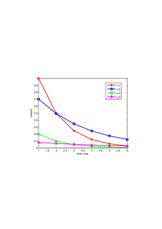
Figure 1: Content value as a function of time.

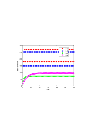
Figure 2: The case of $M=1$.

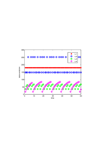
Figure 3: The case of $M=2$.

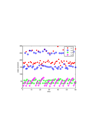
Figure 4: The case of $M=2$ (stochastic model).

9 Conclusions and future works

We have formulated the problem of crawling web sites with ephemeral content as an average reward optimal control problem and have shown that it is indexable. We have found that the Whittle index has a very simple form, which is important for efficient practical implementations. The numerical example demonstrates that the Whittle index policies, unlike the policies suggested in [15], do not generally have a trivial periodic structure. The proposed approach can also be used in the cases when some states are observed. In such cases, the Whittle index will act as a self-tuning mechanism. We are currently working on the adaptive version when some parameters (e.g., the rate of new information arrival) need to be estimated online. One more interesting future research direction is to add to the model the dynamics of the indexing engine.

References

- [1] E. Altman, Constrained Markov Decision Processes, Chapman and Hall / CRC, London, 1999.
- [2] K. Avrachenkov and V. Borkar, “Whittle Index Policy for Crawling Ephemeral Content”, Inria Research Report no.8702, available at https://hal.archives-ouvertes.fr/
- [3] K. Avrachenkov, U. Ayesta, J. Doncel and P. Jacko, “Congestion Control of TCP Flows in Internet Routers by Means of Index Policy”, Computer Networks, vol. 57(17), pp. 3463-3478, 2013.
- [4] K. Avrachenkov, O. Habachi, A. Piunovskiy and Y. Zhang, “Infinite Horizon Optimal Impulsive Control with Applications to Internet Congestion Control”, International Journal of Control, vol. 88(4), pp.703-716, 2015.
- [5] K. Avrachenkov, A. Dudin, V. Klimenok, P. Nain and O. Semenova, “Optimal Threshold Control by the Robots of Web Search Engines with Obsolescence of Documents”, Computer Networks, vol. 55(8), pp. 1880-1893, 2011.
- [6] V.S. Borkar, “Convex Analytic Methods in Markov Decision Processes”, in ‘Handbook of Markov Decision Processes’, (A. Shwartz and E. Feinberg, eds.), Kluwer Academic, New York, 2002, pp. 347-375.
- [7] J. Cho and H. Garcia-Molina, “Synchronizing a Database to Improve Freshness”, In Proceedings of ACM SIGMOD 2000, vol. 29(2), pp. 117-128.
- [8] J. Cho and H. Garcia-Molina, “Effective Page Refresh Policies for Web Crawlers”, ACM Transactions on Database Systems (TODS), vol. 28(4), pp. 390-426.
- [9] J. Cho and A. Ntoulas, “Effective Change Detection Using Sampling”, In Proceedings of VLDB 2002, pp. 514-525.
- [10] A. Goyal, F. Bonchi and L.V. Lakshmanan, “Learning Influence Probabilities in Social Networks”, In Proceedings of ACM WSDM 2010, pp. 241-250, 2010.
- [11] O. Hernández-Lerma and J.-B. Lasserre, Discrete Time Markov Control Processes: Basic Optimality Criteria, Springer Verlag, New York, 1996.
- [12] P. Jacko, Dynamic Priority Allocation in Restless Bandit Models, Lambert Academic Publishing, 188 pages, 2010.
- [13] P. Jacko and B. Sanso, “Congestion Avoidance with Future-Path Information”, in Proceedings of EuroFGI Workshop on IP QoS and Traffic Control, IST Press, pp. 153-160, 2007.
- [14] M. Larranaga, U. Ayesta and I.M. Verloop, “Stochastic and Fluid Index Policies for Resource Allocation Problems”, in Proceedings of IEEE INFOCOM 2015, pp. 1-9.
- [15] D. Lefortier, L. Ostroumova, E. Samosvat and P. Serdyukov, “Timely Crawling of High-quality Ephemeral New Content”, In Proceedings of CIKM 2013, 27 Oct. - 1 Nov., 2013, San Francisco, pp. 745-750.
- [16] Z. Liu and P. Nain, “Optimization Issues in Web Search Engines”, In Handbook of Optimization in Telecommunications, pp. 981-1015, Springer US, 2006.
- [17] K. Liu and Q. Zhao, “Indexability of Restless Bandit Problems and Optimality of Whittle Index for Dynamic Multichannel Access”, IEEE Trans. Info. Theory, vol. 56(11), 2010, pp. 5547-5567.
- [18] T. Moon, W. Chu, L. Li, Z. Zheng and Y. Chang, “Refining Recency Search Results with User Click Feedback”. ArXiv preprint arXiv:1103.3735, 2011.
- [19] J. Nino-Mora and S.S. Villar, “Sensor Scheduling for Hunting Elusive Hiding Targets via Whittle’s Restless Bandit Index Policy”, in Proceedings of NetGCoop 2011, 12-14 Oct., pp. 1-8.
- [20] J.L. Ny, M. Dahleh and E. Feron, “Multi-UAV Dynamic Routing with Partial Observations Using Restless Bandit Allocation Indices”, in Proceedings of American Control Conf. (ACC 2008), 11-13 June 2008, Seattle, pp. 4220-4225.
- [21] C. Olston and M. Najork, “Web Crawling”, In Foundations and Trends in Information Retrieval, vol. 4(3), pp. 175-246, 2010.
- [22] A.B. Piunovskiy, Optimal Control of Random Sequences in Problems with Constraints, Springer, 348 pages, 1997.
- [23] V. Raghunathan, V.S. Borkar, M. Cao and P.R. Kumar, “Index Policies for Real-time Multicast Scheduling for Wireless Bradcast Systems”, in Proceedings of IEEE INFOCOM 2008, 13-18 April 2008, Phoenix, pp. 2243-2251.
- [24] D. Ruiz-Hernandez, Indexable Restless Bandits, VDM Verlag, 2008.
- [25] J. Talim, Z. Liu, P. Nain and E.G. Coffman, Jr., “Controlling the Robots of Web Search Engines”, Performance Evaluation Review, vol. 29(1), pp. 236-244, 2001.
- [26] I.M. Verloop, “Asymptotically Optimal Priority Policies for Indexable and Non-indexable Restless Bandits”, to appear in Annals of Applied Probability, 2015.
- [27] R.R. Weber and G. Weiss, “On an Index Policy for Restless Bandits”, J. Appl. Prob., vol. 27, pp. 637-648, 1990.
- [28] P. Whittle, “Restless Bandits: Activity Allocation in a Changing World”, J. Appl. Prob., vol. 25, pp. 287-298, 1988.