Spin-Mixing Interferometry with Bose-Einstein Condensates

Abstract

Unstable spinor Bose-Einstein condensates are ideal candidates to create nonlinear three-mode interferometers. Our analysis goes beyond the standard SU(1,1) parametric approach and therefore provides the regime of parameters where sub-shot-noise sensitivities can be reached with respect to the input total average number of particles. Decoherence due to particle losses and finite detection efficiency are also considered.

Interferometers provide the most precise measurements in physics Note ; Hariharan (2003); Cronin et al. (2009); *SchnabelNATCOMM2010. Hence, there is an urgent demand for novel theoretical proposals and experimental techniques aimed at further increasing their sensitivity. Most of the current atomic and optical interferometers are made of linear devices such as beam splitters and phase shifters. Their phase uncertainty is fundamentally bounded by the shot-noise limit $\Delta\theta\sim 1/\sqrt{\bar{n}}$, when using probe states made of average $\bar{n}$ uncorrelated particles Pezzè and Smerzi (2009); Giovannetti et al. (2006). It has been clarified that overcoming this bound requires engineering proper particle-entangled states Pezzè and Smerzi (2009) (see  Refs. Giovannetti et al. (2011); Toth ; Pezzè and Smerzi (2014) for reviews). Using such states, sub-shot-noise (SSN) phase uncertainties have been demonstrated in several recent proof-of-principle experiments with atoms Gross et al. (2010); Ockeloen et al. (2013); Muessel et al. (2014); Strobel et al. (2014); Lücke et al. (2011); Leroux et al. (2010); *AppelPNAS2009; *BohnetNATPHOT2014 and photons Nagata et al. (2007); *XiangNATPHOT2011; *KrischekPRL2011; *KacprowiczNATPHOT2010; *AfekSCIENCE2010. Yet, noise and decoherence limit the creation and use of quantum correlations Escher et al. (2011); *DemkowiczNATCOMM2012. It is therefore crucial to search for alternative schemes where probe states are classical and quantum correlations useful to reach SSN sensitivities are created inside the interferometer Gross et al. (2010); Riedel et al. (2010); Ockeloen et al. (2013); Muessel et al. (2014).

In this Letter, we show that the coherent spin-mixing dynamics (SMD) in a spinor Bose-Einstein condensate (BEC) Ho (1998); *OhmiPRL1998; Stamper-Kurn and Ueda (2013) can be exploited to realize a nonlinear three-mode interferometer, as shown in Fig. 1. The SMD consists of binary collisions that coherently transfer correlated pairs of trapped atoms with opposite magnetic moment Pu and Meystre (2000); *DuanPRL2000 from the $m_{f}=0$ to the $m_{f}=\pm 1$ hyperfine modes, and vice versa. The probe state of the interferometer is classical, given by a condensate initially prepared in the $m_{f}=0$ mode, and quantum correlations are created by the SMD. We first study the interferometer in the mean-field limit, the $m_{f}=0$ mode operator being replaced by a $c$-number. This analysis is valid for a large number of particles and low transfer rates. In this case, the interferometer operations belong to the SU(1,1) group and it is possible to obtain analytical predictions for the phase sensitivity. In optical systems, where transfer rates are rather low, the probe state needs to be very intense and the SU(1,1) approach is well justified Yurke et al. (1986). SU(1,1) optical interferometry has been theoretically discussed Yurke et al. (1986); Plick et al. (2010); Ou (2012); Marino et al. (2012) and recently experimentally realized Hudelist et al. (2014). In contrast, experiments with spinor BECs Lücke et al. (2011); Gross et al. (2011); Hamley et al. (2012); *GervingNATCOMM2013 can be performed well outside the mean-field regime, with probe states of a relatively small number of particles and – thanks to strong nonlinearities – comparatively high transfer rates. We have thus also implemented a full three-mode quantum analysis. Within this framework, we can rigorously provide phase sensitivity bounds with respect to the average total number of particles $\bar{n}$ in input. For realistic values of $\bar{n}$, including particle losses and finite detection efficiency, SSN is obtained in a regime where quantum corrections to the mean-field picture are important.

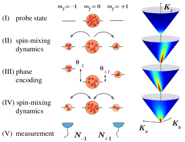
Figure 1: Left: scheme of spin-mixing interferometry with spinor BEC, here represented in the $f=1$ manifold. Right: when the $m_{f}=0$ mode is treated parametrically (mean-field approach), the interferometer operations can be visualized on a hyperbolic surface by projecting the transformed state over SU(1,1) coherent states Yurke et al. (1986); Brif et al. (1996).

Spin-mixing interferometry with BECs. The protocol outlined in Fig. 1 follows five steps: (I) probe state preparation – we consider empty $m_{f}=\pm 1$ modes and a BEC of average $\bar{n}$ atoms in the $m_{f}=0$ mode, (II) a first SMD, (III) phase encoding, and (IV) a second SMD. Finally (V) the atoms are released from the trap: the three magnetic modes are spatially separated and the particle number is measured by imaging the atomic clouds.

A standard description of the SMD is obtained in the single-mode approximation Kawaguchi and Ueda (2012): the condensate spatial wave function $\psi(\bm{r})$ in the $m_{f}=\pm 1$ modes is assumed to be the same as in the $m_{f}=0$ mode and it is given by the solution of the Gross-Pitaevskii equation in the trapping potential Law et al. (1998). This approximation is justified for a relatively low atom number $\bar{n}\lesssim 10^{5}$, and tight confinement, when the spin healing length is larger than the size of the atomic cloud. These conditions are fulfilled in typical experimental setups Stamper-Kurn and Ueda (2013). The field operators are thus approximated by $\hat{\Psi}_{i}(\bm{r})=\psi(\bm{r})\hat{a}_{i}$, where $\hat{a}_{i}$ ($\hat{a}^{\dagger}_{i}$) are annihilation (creation) operators for modes $i=m_{f}=0,\pm 1$ obeying the boson commutation relations $[\hat{a}_{i},\hat{a}_{j}^{{\dagger}}]=\delta_{i,j}$ ($\hat{N}_{i}=\hat{a}_{i}^{\dagger}\hat{a}_{i}$ is the particle number operator). Up to terms proportional to the constant total particle number $\hat{N}=\hat{N}_{-1}+\hat{N}_{0}+\hat{N}_{+1}$, the many-body Hamiltonian describing the SMD in a dilute atomic cloud is Law et al. (1998)

$$\hat{H}_{\rm SMD} = \chi\hbar\,(e^{2i\phi}\hat{a}_{0}^{{\dagger}}\hat{a}_{0}^{{\dagger}}\hat{a}_{+1}\hat{a}_{-1}+e^{-2i\phi}\hat{a}_{0}\hat{a}_{0}\hat{a}_{+1}^{{\dagger}}\hat{a}_{-1}^{{\dagger}})+$$ (1)

$$+ \chi\hbar\,\big{(}\hat{N}_{0}-\tfrac{1}{2}\big{)}(\hat{N}_{+1}+\hat{N}_{-1}).$$

The first term is identical to four-wave mixing in nonlinear optics Yurke et al. (1986); Scully and Zubairy (1997), where $\phi$ is the relative phase between the $m_{f}=0$ and $m_{f}=\pm 1$ modes. The second term in Eq. (1) is a mean-field shift. The coupling $\chi=\frac{4\pi\hbar}{3M}(c_{2}-c_{0})\int d^{3}\bm{r}|\psi(\bm{r})|^{4}$ depends on the $s$-wave scattering lengths $c_{0}$ and $c_{2}$ of two bosons of mass $M$ scattering in the total spin channels $F=0$ and $F=2$, respectively Ho (1998); Ohmi and Machida (1998); Widera et al. (2006). We indicate as $(\chi t,\phi)_{1}$ [$(\chi t,\phi)_{2}$] the parameters for the first [second] SMD. Experimentally, the SMD can be accurately controlled via microwave dressing Stamper-Kurn and Ueda (2013) and, in particular, switched off during phase acquisition. Neglecting interaction between particles during this stage, the (linear) phase shift Hamiltonian is

$$\hat{H}_{\rm PS}=\hbar q\big{(}\hat{N}_{+1}+\hat{N}_{-1}\big{)},$$ (2)

where $\hbar q$ is the energy difference between the $m_{f}=0$ and the $m_{f}=\pm 1$ modes, see Fig. 1. The unitary transformation $e^{-i\hat{H}_{\rm PS}t_{\rm PS}/\hbar}$ encodes the phase shift $\theta=\theta_{+1}+\theta_{-1}=2qt_{\rm PS}$, where $\theta_{\pm 1}$ are the phases accumulated by the atoms in the $m_{f}=\pm 1$ modes, relative to the ones in the $m_{f}=0$ mode, during a time $t_{\rm PS}$. For instance, the signal can be the second-order Zeeman shift due to a sufficiently strong magnetic field. Note that the first-order Zeeman shift, proportional to the net magnetization (equal to zero for our initial state), is conserved.

The phase shift is estimated by measuring the number of particles in the $m_{f}=\pm 1$ modes at the end of the interferometric sequence. We calculate the phase uncertainty as $\Delta\theta_{\rm CR}=1/\sqrt{mF(\theta)}$, the Cramér-Rao lower bound Helstrom (1976); Giovannetti et al. (2011); Pezzè and Smerzi (2014), where $m$ accounts for the repetition of independent measurements,

$$F(\theta)\equiv\sum_{N_{\pm 1}=0}^{\infty}\frac{1}{P(N_{\pm 1}|\theta)}\bigg{(}\frac{\mathrm{d}P(N_{\pm 1}|\theta)}{\mathrm{d}\theta}\bigg{)}^{2}$$ (3)

is the Fisher information (FI) and $P(N_{\pm 1}|\theta)$ is the conditional probability to measure $N_{\pm 1}$ particles given the phase shift $\theta$. $\Delta\theta_{\rm CR}$ is a saturable lower bound of phase uncertainty Giovannetti et al. (2011); Helstrom (1976); Pezzè and Smerzi (2014). The FI can be experimentally extracted following the method demonstrated in Strobel et al. (2014). Alternatively, we can calculate the phase uncertainty from the error propagation, $\Delta\theta_{\rm ep}=\frac{(\Delta\hat{N}_{\pm 1})_{\rm out}}{|\mathrm{d}\langle\hat{N}_{\pm 1}\rangle_{\rm out}/\mathrm{d}\theta|}$, where $\langle\hat{N}_{\pm 1}\rangle_{\rm out}$ is the average number of particles in output and $(\Delta\hat{N}_{\pm 1})^{2}_{\rm out}$ is the corresponding variance. This method is experimentally feasible but not always optimal: we have $\Delta\theta_{\rm ep}/\sqrt{m}\geq\Delta\theta_{\rm CR}$, in general Pezzè and Smerzi (2009, 2014).

Mean-field approach. When the initial condensate contains a large number of particles and is weakly affected by the SMD, we can study the interferometer operations by replacing $\hat{a}_{0}$ with $\sqrt{\bar{n}}$. We introduce the operators $\hat{K}_{x}=\frac{1}{2}(\hat{a}_{+1}^{\dagger}\hat{a}_{-1}^{\dagger}+\hat{a}_{+1}\hat{a}_{-1})$, $\hat{K}_{y}=\frac{1}{2i}(\hat{a}^{\dagger}_{+1}\hat{a}_{-1}^{\dagger}-\hat{a}_{+1}\hat{a}_{-1})$, $\hat{K}_{z}=\frac{1}{2}(\hat{a}^{\dagger}_{+1}\hat{a}_{+1}+\hat{a}_{-1}^{{\dagger}}\hat{a}_{-1}+1)$, which belong to the SU(1,1) group and satisfy $[\hat{K}_{x},\hat{K}_{y}]=-i\hat{K}_{z}$, $[\hat{K}_{y},\hat{K}_{z}]=i\hat{K}_{x}$ and $[\hat{K}_{z},\hat{K}_{x}]=i\hat{K}_{y}$ Yurke et al. (1986); Wódkiewicz and Eberly (1985). Equations (1) and (2) thus become, up to a constant term, $\hat{H}_{\rm SMD}=(2\bar{n}-1)\chi\hbar\hat{K}_{z}+2\bar{n}\chi\hbar(\hat{K}_{x}\cos 2\phi+\hat{K}_{y}\sin 2\phi)$ and $\hat{H}_{\rm PS}=2\hbar q\hat{K}_{z}$, respectively. The interferometer protocol starts with vacuum in the $m_{f}=\pm 1$ modes [Fig. 1(I)]. The first SMD $e^{-i\hat{H}_{\rm SMD}t/\hbar}$ [$(\chi t)_{1}=\chi t$, $\phi_{1}=0$] generates a Lorentz boost Leslie et al. (2009); Klempt et al. (2010) that amplifies the population in the $m_{f}=\pm 1$ modes

$$\mathcal{N}(t)=\frac{8\bar{n}^{2}}{4\bar{n}-1}\sinh^{2}\Big{(}\frac{\sqrt{4\bar{n}-1}}{2}\chi t\Big{)},$$ (4)

where $\mathcal{N}\equiv\langle\hat{N}_{+1}+\hat{N}_{-1}\rangle_{\rm SMD}$ [Fig. 1(II)]. The mean-field description is thus valid when Note (2)

$$\chi t\to 0,\,\bar{n}\to+\infty,\qquad\text{such that}\,\,\,0<\chi t\sqrt{\bar{n}}\ll 1.$$ (5)

The SMD generates a thermal distribution of perfectly correlated atom pairs in the $\pm 1$ modes Pu and Meystre (2000); Duan et al. (2000): the two-mode squeezed-vacuum state Scully and Zubairy (1997), with variance $(\Delta\hat{N}_{\pm 1})_{\rm SMD}^{2}=\frac{\mathcal{N}}{2}(\frac{\mathcal{N}}{2}+1)$. The transformation $e^{-i\hat{H}_{\rm PS}t_{\rm PS}/\hbar}$ rotates the state around the $z$ axis of an angle $\theta$ [Fig. 1(III)]. The final operation is a second SMD. This can be implemented either as an inverse Lorentz boost $e^{i\hat{H}_{\rm SMD}t/\hbar}$ [i.e. $(\chi t)_{2}=-(\chi t)_{1}$, $\phi_{2}=0$, as in Fig. 1(IV)], or by applying a $\pi/2$ phase shift to the $m_{f}=0$ mode followed by the transformation $e^{-i\hat{H}_{\rm SMD}t/\hbar}$ [i.e. $(\chi t)_{2}=(\chi t)_{1}$, $\phi_{2}=\pi/2$]. The latter is easier to be realized experimentally Note (5). In both cases, the conditional probabilities are

$$P(N_{\pm 1}|\theta)=\frac{2[\mathcal{N}(\mathcal{N}+2)(1-\cos\theta)]^{N_{\pm 1}}}{[\mathcal{N}(\mathcal{N}+2)(1-\cos\theta)+2]^{N_{\pm 1}+1}}.$$ (6)

A direct calculation of Eq. (3) yields

$$F(\theta)=\frac{\mathcal{N}(\mathcal{N}+2)}{\mathcal{N}(\mathcal{N}+2)\sin^{2}\frac{\theta}{2}+1}\cos^{2}\tfrac{\theta}{2},$$ (7)

where $\mathcal{N}$ is given by Eq. (4). The FI reaches its maximum at $\theta=0$. In this case, if $(\chi t)_{2}=-(\chi t)_{1}$ the two SMDs exactly compensate and the output $m_{f}=\pm 1$ modes are empty. Note also that $\langle\hat{N}_{\pm 1}\rangle_{\rm out}=\mathcal{N}\big{(}\mathcal{N}+2\big{)}\sin^{2}\tfrac{\theta}{2}$ and $(\Delta\hat{N}_{\pm 1})^{2}_{\rm out}=(\Delta\hat{N})^{2}_{\rm SMD}\sin^{2}\tfrac{\theta}{2}[(\Delta\hat{N})^{2}_{\rm SMD}\sin^{2}\tfrac{\theta}{2}+1]$: error propagation saturates the Cramér-Rao lower bound, $\Delta\theta_{\rm ep}=\Delta\theta_{\rm CR}$. At $\theta=0$, we obtain $\Delta\theta_{\rm CR}=1/\sqrt{m\mathcal{N}(\mathcal{N}+2)}$, which is below the shot noise, $\Delta\theta_{\rm CR}<1/\sqrt{m\mathcal{N}}$, calculated considering only the average population in $m_{f}=\pm 1$ after the first SMD Yurke et al. (1986); Hudelist et al. (2014). We notice here that the shot noise should be calculated with respect to the total resources, i.e. the total average number of particles $\bar{n}$ in the input state. However, such an analysis is impossible within the SU(1,1) framework.

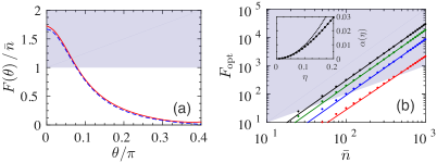
Figure 2: (a) The FI as a function of $\theta$ (solid red line) and error propagation $1/(\Delta\theta)^{2}_{\rm ep}$ (dashed blue line). The shaded area is $F(\theta)>\bar{n}$. Here $\bar{n}=50$ and $\eta=0.2$. (b) $F_{\rm opt}$ as a function of $\bar{n}$. Dots are numerical results and solid lines are quadratic fits to the data: $F_{\rm opt}=\alpha(\eta)\bar{n}^{2}$, for $\bar{n}\gg 1$. Here $\eta=0.05$ (red), $0.1$ (blue), $0.15$ (green) and $0.2$ (black). The shaded area is $F_{\rm opt}>\bar{n}$. The inset shows $\alpha(\eta)$ as a function of $\eta$ (dots). The solid line is a quadratic fit $\alpha(\eta)=\eta^{2}-1.31\eta^{3}$; the dotted line is $\alpha(\eta)=\eta^{2}$.

Full quantum approach. We have thus performed a full three-mode quantum analysis, investigating the regime of parameters beyond Eq. (5). Thanks to the symmetry of the Hamiltonian (1), we can restrict ourselves to the Hilbert subspace spanned by Fock states $\{|N_{-1},N_{0},N_{+1}\rangle\equiv|k,M-2k,k\rangle\}$, with $0\leq k\leq\left\lfloor\frac{M}{2}\right\rfloor$ Mias et al. (2008); Goldstein and Meystre (1999). We take $\hat{\rho}=\sum_{M=0}^{+\infty}\frac{\bar{n}^{M}e^{-\bar{n}}}{M!}|0,M,0\rangle\langle 0,M,0|$ as the (input) probe state.

We numerically calculate $F(\theta)$ for different values of the parameters $\bar{n}$, $\eta$ and $\theta$, where $\eta\equiv\langle\hat{N}_{+1}+\hat{N}_{-1}\rangle_{\rm SMD}/\bar{n}$ is the fraction of particles transferred from the $m_{f}=0$ mode to the $m_{f}=\pm 1$ modes after the first SMD. We mainly focus on the case $(\chi t)_{2}=-(\chi t)_{1}$ which, as shown below, is optimal. Overall, the FI as a function of $\theta$ shows a behavior qualitatively similar to Eq. (7), with a maximum at $\theta=0$, see Fig. 2(a). A first important result is that, for proper values of $\eta$, the FI can be larger than $\bar{n}$ or, equivalently, $\Delta\theta_{\rm CR}<1/\sqrt{m\bar{n}}$. In other words, it is possible to attain SSN uncertainties with respect to the average input number of particles.

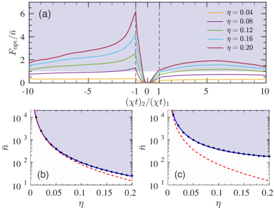
Figure 3: (a) $F_{\rm opt}$ as a function of the ratio $(\chi t)_{2}/(\chi t)_{1}$. Solid lines refer to different values of $\eta$. Here $\bar{n}=200$. Panels (b) and (c) show the phase-sensitivity portrait in the $(\eta,\bar{n})$-parameter space for $(\chi t)_{1}=-(\chi t)_{2}$ and $(\chi t)_{1}=(\chi t)_{2}$, respectively. SSN phase uncertainties are obtained for $\bar{n}$ larger than a critical value $\bar{n}_{\rm cr}(\eta)$ (dots, the solid line being a guide to the eye). The dashed red line in both panels is $\bar{n}_{\rm cr}(\eta)=(1-2\eta)/\eta^{2}$, obtained from a mean-field calculation, which agrees with the numerics in the limit (5). In all panels, the shaded area indicates SSN.

A scaling analysis of the FI as a function of $\bar{n}$ at the optimal point $\theta=0$ [we indicate $F_{\rm opt}\equiv\max_{\theta}F(\theta)$] shows that $F_{\rm opt}\approx\alpha(\eta)\bar{n}^{2}$ asymptotically in $\bar{n}$ (in our simulations $\bar{n}\lesssim 1000$), see Fig. 2(b). A fit gives $\alpha(\eta)\approx\eta^{2}(1-1.3\eta)$ in the case $(\chi t)_{2}/(\chi t)_{1}=-1$ [see the inset of Fig. 2(b)]. We thus conclude that $\Delta\theta_{\rm CR}\sim 1/\bar{n}$ with a prefactor depending on $\eta$.

Figure 3 is the main result of this Letter. In panel (a) we show $F_{\rm opt}$ as a function of the ratio $(\chi t)_{2}/(\chi t)_{1}$, for different values of $\eta$. For relatively large $\eta$, outside the mean-field regime, the curves are asymmetric around zero. The optimal interferometer configuration is reached for $(\chi t)_{2}=-(\chi t)_{1}$, but SSN can be also obtained for positive values of $(\chi t)_{1}/(\chi t)_{2}$: inverting the sign of $\chi$ in the second SMD transformation, which might be experimentally difficult, is not necessary to reach SSN sensitivities. Figures 3(b) and 3(c) show the regime of parameters where SSN can be achieved, for $(\chi t)_{2}=-(\chi t)_{1}$ and $(\chi t)_{2}=(\chi t)_{1}$, respectively. For fixed $\eta$, a critical value $\bar{n}_{\rm cr}(\eta)$ exists such that $\Delta\theta_{\rm CR}\leq 1/\sqrt{m\bar{n}}$, for $\bar{n}>\bar{n}_{\rm cr}(\eta)$. Deviations from the mean-field prediction, $\bar{n}_{\rm cr}(\eta)=(1-2\eta)/\eta^{2}$, can be appreciated for small $\bar{n}$, especially for $(\chi t)_{2}/(\chi t)_{1}>0$, and are relevant in current BEC experiments Gross et al. (2011); Hamley et al. (2012); Gerving et al. (2013); Lücke et al. (2011).

Particle loss and finite detection efficiency. According to Eq. (4), the SMD is unaffected by decoherence processes that happen on time scales much longer than $\sim 1/(\chi\sqrt{\bar{n}})$. For sufficiently large $\bar{n}$ and fast phase encoding, the nonlinear interferometer thus appears to be robust to one-body losses (relevant for the spin-mixing dynamics in the $f=1$ manifold Peise et al. (2015)). In fact, this dissipation source – due to inelastic collisions of the ultracold trapped atoms with the background thermal cloud, or by off-resonant light scattering in a dipole trap – has a density-independent rate. Conversely, recombination losses – whose rate depends on $\bar{n}$ – may strongly affect the interferometer sensitivity. We have thus simulated two-body losses in the $m_{f}=0$ mode (relevant for the spin-mixing dynamics in the $f=2$ manifold Gross et al. (2011); Lücke et al. (2011)) using a Monte Carlo wave-function approach Mølmer et al. (1993); *LiPRL2008. Let $\gamma$ indicate the depletion rate during the SMD operation [i.e. $\langle\hat{N}_{0}(t)\rangle=\bar{n}/(1+2\gamma t\bar{n})$ for $\chi=0$]. Figure 4(a) shows the regime of parameters $(\eta,\bar{n})$ where SSN sensitivities can be found. The SSN region shrinks when increasing $\gamma/\chi$ and, in particular, no SSN is found for $\gamma/\chi\gtrsim 0.04$. The branch structure of the SSN regions is explained by the characteristic effects induced by particle losses shown in Figs. 4(b) and 4(c). In Fig. 4(b) we plot $\eta$ as a function of time, for different values of $\gamma/\chi$. Losses decrease the transfer rate and place an upper bound to the achievable $\eta$. In Fig. 4(c) we show the FI as a function of $\bar{n}$. For $\bar{n}\ll(\chi/2\gamma)^{2}$, the effect of losses can be neglected and we recover the scaling $F_{\rm opt}\propto(\eta\bar{n})^{2}$ of the noiseless case. For $\bar{n}\gtrsim(\chi/2\gamma)^{2}$ losses dominate and the sensitivity quickly degrades. For instance, in typical experiments with ⁸⁷Rb in the $f=2$ manifold, the coupling strength is $\chi\approx 0.5$ Hz and we estimate a ratio $\gamma/\chi\approx 10^{-3}-10^{-2}$, well within our explored range.

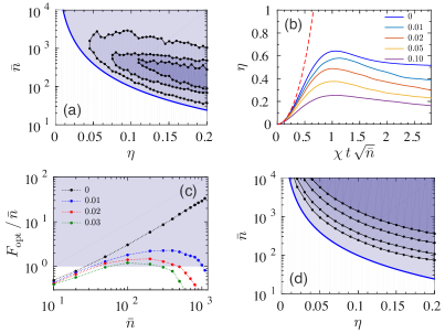
Figure 4: (a) SSN region in $(\eta,\bar{n})$-parameter space including two-body losses in the $m_{f}=0$ mode, with loss parameter $\gamma/\chi=0.01$, $0.02$ and $0.03$ (from outer to inner regions). The thick blue line, for $\gamma=0$, is the same as the solid line in Fig. 3. (b) $\eta$ as a function of time, for different values of $\gamma/\chi$ (solid lines). Here $\bar{n}=200$ and the dashed line is Eq. (5). (c) $F_{\rm opt}$ as a function of $\bar{n}$ for $\eta=0.2$ and different values of $\gamma/\chi$. Dotted lines are guides to the eye. (d) SSN region in $(\eta,\bar{n})$-parameter space obtained for detection noise $\sigma=1$, $2$, $5$, $10$ (from outer to inner regions). The thick blue line ($\sigma=0$) corresponds to the solid line in Fig. 3. In panels (a) and (d) the dots are numerical results and the solid lines are guides to the eye.

To model finite detection efficiency we consider a Gaussian convolution of the ideal output probabilities Note (4); Pezzè and Smerzi (2013). Results for different values of the detection noise $\sigma$ are shown in Fig. 4(d). In typical experiments $\sigma\approx 10$, while a high detection sensitivity $\sigma\approx 1$ has been discussed in Ref. Muessel et al. (2014). In the regime (5) we can evaluate the FI from a convolution of probabilities (6). This allows for semianalytical calculations giving, to the leading order in $1/\eta$ and for $\sigma\gtrsim 1$, $\bar{n}_{\rm cr}(\eta)\approx 2\sigma/\eta^{2}$, which agrees with numerical calculations for $\bar{n}\to+\infty$ and $\eta\to 0$. It predicts that $n_{\rm cr}(\eta)$ shifts toward larger values when increasing $\sigma$, an expected behavior Marino et al. (2012) that qualitatively holds also outside the mean-field regime.

Conclusions. We have studied a nonlinear three-mode interferometer with spinor BECs. The nonlinear spin-mixing dynamics not only splits the initial cloud but, differently from a linear beam splitter, it also creates, at the same time, quantum correlations among particles, necessary to overcome the shot-noise limit. Therefore, differently from linear interferometers, the nonlinear scheme discussed in this Letter can reach SSN phase uncertainties with classically correlated probe states. Accurate predictions of the phase sensitivity require a full three-mode quantum analysis, beyond the SU(1,1) (mean-field) approach. We have performed such an analysis and showed that it is possible to overcome the shot-noise limit with respect to the total average number of atoms in input. We also provide the regime of parameters where sub-shot-noise uncertainties can be achieved, including losses and finite detection efficiencies. Our results pave the way to atomic ultrasensitive spin-mixing interferometry Note (5).