Effective Interactions in Active Brownian Suspensions

Abstract

Active colloids exhibit persistent motion, which can lead to motility-induced phase separation (MIPS). However, there currently exists no microscopic theory to account for this phenomenon. We report a first-principles theory, free of fit parameters, for active spherical colloids, which shows explicitly how an effective many-body interaction potential is generated by activity and how this can rationalize MIPS. For a passively repulsive system the theory predicts phase separation and pair correlations in quantitative agreement with simulation. For an attractive system the theory shows that phase separation becomes suppressed by moderate activity, consistent with recent experiments and simulations, and suggests a mechanism for reentrant cluster formation at high activity.

Active colloidal particles in suspension are currently the subject of considerable attention, due largely to their ability to model self-organisation phenomena in biological systems, but also as a new branch of fundamental research in nonequilibrium statistical mechanics: assemblies of active colloids are intrinsically out-of-equilibrium systems. In contrast to their passive counterparts, active colloids undergo both solvent induced Brownian motion and a self-propulsion which requires a continual consumption of energy from the local environment. Several idealized experimental model systems have been developed, such as catalytic Janus particles lyderic2010 ; erbe2008 ; howse2007 , colloids with artificial flagella flagella2005 and light activated particles palacci2013 . The understanding of active systems has been further aided by the development of simple theoretical models, which aim to capture the essential physical mechanisms and which have been used to study e.g. bacteria, cells or filaments in the cytoskeleton collective_motion2012 ; ramaswamy2010 ; romanczuk2012 ; cates_bacteria2012 .

Active particles are characterised by a persistent motion, which can lead to ‘self trapping’ dynamics and a rich variety of related collective phenomena collective_motion2012 ; ramaswamy2010 ; romanczuk2012 ; cates_bacteria2012 ; cates_tailleur2014 . Even the simplest models of active spherical particles with purely repulsive interactions can display the phenomenon of motility-induced phase separation (MIPS) cates_tailleur2014 . In many respects, MIPS resembles the equilibrium phase separation familiar from passive systems with an attractive component to the interaction potential (e.g. the Lennard-Jones potential) tailleur2008 ; fily2012 ; stenhammar2013 ; redner2013 ; levis_berthier2014 . This apparent similarity has motivated several recent attempts to map an assembly of active particles onto a passive equilibrium system, interacting via an effective attraction (usually taken to be a very short range sticky-sphere potential schwarz-linek2012 ; bocquetPRX_2014 ). Despite the intuitive appeal of mapping to an equilibrium system, there exists no systematic theoretical approach capable of predicting an effective equilibrium potential directly from the bare interactions.

Our current understanding of MIPS has largely been gained through either simulation fily2012 ; redner2013 ; stenhammar2013 ; levis_berthier2014 ; wysocki2014 or phenomenological theory tailleur2008 ; cates2013 ; stenhammar2013 ; cates_tailleur2014 . The phenomenological theory is based on an equation for the coarse-grained density, featuring a local speed and a local orientational relaxation time. Although the precise relationship between these one-body fields and the interparticle interaction potential remains to be clarified, some progress in this direction has been made bialke2013 . On a more microscopic level, it has recently been shown that a general system of active particles does not have an equation of state cates_kardar , due to the influence of the confining boundaries, however, one can be recovered for the special case of active Brownian spheres cates_kardar ; takatori .

Here we report a first-principles theory for systems of active Brownian spheres, which demonstrates explicitly how an effective many-body interaction potential is induced by activity. An appealing feature of this approach is that intuition gained from equilibrium can be used to understand the steady-state properties of active systems. The required input quantities are the passive (‘bare’) interaction potential, the rotational diffusion coefficient and the particle propulsion speed. The theory generates as output the static correlation functions and phase behaviour of the active system. For a repulsive bare interaction, activity generates an attractive effective pair potential, thus providing an intuitive explanation for the MIPS observed in simulations fily2012 ; levis_berthier2014 ; stenhammar2014 . For an attractive bare potential, we find that increasing activity first reduces the effective attraction, consistent with the experiments of Schwarz-Linek et al. schwarz-linek2012 , before leading at higher activity to the development of a repulsive potential barrier. We speculate that this barrier may be related to the reentrant phase behaviour observed in simulation by Redner et al. redner2013 .

The paper will be structured as follows: In §I we specify the microscopic dynamics and describe how to eliminate orientational degrees of freedom. From the resulting coarse-grained, non-Markovian Langevin equation we derive a Fokker-Planck equation for the positional degrees of freedom, from which we identify an effective pair potential. In §II we employ the effective pair potential in an equilibrium integral equation theory and investigate the structure and phase behaviour of both repulsive and attractive bare potentials. In the former case we predict MIPS, whereas in the latter case phase separation is suppressed by activity. Finally, in §III we discuss our findings and provide an outlook for future research.

I Theory

I.1 Microscopic dynamics

We consider a three dimensional system of $N$ active, interacting, spherical Brownian particles with spatial coordinate $\boldsymbol{r}_{i}$ and orientation specified by an embedded unit vector $\boldsymbol{p}_{i}$. Each particle experiences a self propulsion of speed $v_{0}$ in its direction of orientation. Omitting hydrodynamic interactions the particle motion can be modelled by the overdamped Langevin equations

$$\dot{\boldsymbol{r}}_{i}=v_{0}\,\boldsymbol{p}_{i}+\gamma^{-1}\boldsymbol{F}_{i}+\boldsymbol{\xi}_{i},$$ (1)

$$\dot{\boldsymbol{p}}_{i}=\boldsymbol{\eta}_{i}\times\boldsymbol{p}_{i},$$ (2)

where $\gamma$ is the friction coefficient and the force on particle $i$ is generated from the total potential energy according to $\boldsymbol{F}_{i}\!=\!-\nabla_{i}U_{N}$. The stochastic vectors $\boldsymbol{\xi}_{i}(t)$ and $\boldsymbol{\eta}_{i}(t)$ are Gaussian distributed with zero mean and have time correlations $\langle\boldsymbol{\xi}_{i}(t)\boldsymbol{\xi}_{j}(t^{\prime})\rangle=2D_{t}\boldsymbol{1}\delta_{ij}\delta(t-t^{\prime})$ and $\langle\boldsymbol{\eta}_{i}(t)\boldsymbol{\eta}_{j}(t^{\prime})\rangle=2D_{r}\boldsymbol{1}\delta_{ij}\delta(t-t^{\prime})$, where $D_{t}$ and $D_{r}$ are the translational and rotational diffusion coefficients.

Equations (1) and (2) are convenient for simulation, but are perhaps not the most suitable starting point for developing a first-principles microscopic theory. For a homogeneous system, averaging over the angular degrees of freedom generates a coarse-grained equation fily2012

$$\dot{\boldsymbol{r}}_{i}(t) =\gamma^{-1}\boldsymbol{F}_{i}(t)+\boldsymbol{\xi}_{i}(t)+\boldsymbol{\chi}_{i}(t),$$ (3)

where $\boldsymbol{\chi}_{i}(t)$ is a Markov process with zero mean and where the time correlation function is given by

$$\langle\boldsymbol{\chi}_{i}(t)\,\boldsymbol{\chi}_{j}(t^{\prime})\rangle=\frac{v_{0}^{2}}{3}e^{-2D_{r}|t-t^{\prime}|}\boldsymbol{1}\delta_{ij}.$$ (4)

The average in (4) is over both noise and initial orientation. The distribution of $\boldsymbol{\chi}_{i}(t)$ is Gaussian to a good approximation. This point and further technical details of the coarse graining are discussed in Appendix A. Equation (3) provides a mean-field level of description, which deviates from the exact equations (1) and (2) by neglecting the coupling of fluctuations in orientation and positional degrees of freedom.

The Langevin equation (3) describes a non-Markovian process, which approximates the stochastic time evolution of the positional degrees of freedom. The persistent motion of active particles is here encoded by the exponential decay of the time correlation (4), with persistence time $\tau_{p}\!=\!(2D_{r})^{-1}$​. For small $\tau_{p}$ the time correlation becomes $\langle\boldsymbol{\chi}_{i}(t)\boldsymbol{\chi}_{j}(t^{\prime})\rangle=2D_{a}\boldsymbol{1}\delta_{ij}\delta(t-t^{\prime})$ and the dynamics reduce to that of an equilibrium system with diffusion coefficient $D_{t}+D_{a}$, where $D_{a}\!=\!v_{0}^{2}/(6D_{r})$. This limit is realized when $\tau_{p}$ is shorter than the mean free time between collisions, i.e. in a dilute suspension. To treat finite densities requires an approach which deals with persistent trajectories. With this aim, we adopt (3) as the starting point for contructing a closed theory.

I.2 Fokker-Planck equation

A stochastic process driven by colored noise, such as that described by equation (3), is always non-Markovian. Consequently, it is not possible to derive an exact Fokker-Planck equation for the time evolution of the probability distribution vankampen1976 . Nevertheless, an approximate Fokker-Planck description capable of making accurate predictions can usually be found. The approximate Fokker-Planck equation implicitly defines a Markov process which best approximates the process of physical interest (although precisely what constitutes the ‘best’ approximation remains a matter of debate). From the extensive literature on this subject (see vankampen1976 ; vankampen1998 ; faetti1988 and references therein) has emerged a powerful method due to Fox fox1986 ; fox_weak1986 , in which a perturbative expansion in powers of correlation time is partially resummed using functional calculus. The resulting Fokker-Planck equation is most accurate for short correlation times (‘off white’ noise vankampen1998 ) and for one-dimensional models makes predictions in good agreement with simulation data faetti1988 .

We now consider applying the method of Fox fox1986 ; fox_weak1986 to equation (3). This approach consists of first formulating the configurational probability distribution as a path (functional) integral and then making a time-local, Markovian approximation to this quantity. Technical details of the method are given in Appendix B. Fox’s approach was originally developed to treat one-dimensional problems fox1986 ; fox_weak1986 , however the generalization to three dimensions is quite straightforward. This enables us to directly obtain the following Fokker-Planck equation

$$\partial_{t}\Psi(\boldsymbol{r}^{N}\!\!,t)=-\sum_{i=1}^{N}\nabla_{i}\cdot\boldsymbol{J}_{i}(\boldsymbol{r}^{N}\!\!,t),$$ (5)

where $\Psi(\boldsymbol{r}^{N}\!\!,t)$ is the configurational probability distribution. Within the generalized Fox approximation the many-body current is given by

$$\boldsymbol{J}_{i}(\boldsymbol{r}^{N}\!\!,t)=-D_{i}(\boldsymbol{r}^{N})\left[\,\nabla_{i}-\beta\boldsymbol{F}_{i}^{\rm eff}(\boldsymbol{r}^{N})\,\right]\Psi(\boldsymbol{r}^{N}\!\!,t),$$ (6)

where $\beta\!\equiv\!(k_{B}T)^{-1}$. The diffusion coefficient is given by

$$D_{i}(\boldsymbol{r}^{N})=D_{t}+D_{a}\left(1+\frac{\tau\nabla_{i}\!\cdot\!\beta\boldsymbol{F}_{i}(\boldsymbol{r}^{N})}{1-\tau\nabla_{i}\!\cdot\!\beta\boldsymbol{F}_{i}(\boldsymbol{r}^{N})}\right),$$ (7)

where we have defined a dimensionless persistence time, $\tau\!=\!\tau_{p}D_{t}/d^{2}$. The effective force is given by

$$\boldsymbol{F}_{i}^{\rm eff}(\boldsymbol{r}^{N})= \frac{1}{\mathcal{D}_{i}(\boldsymbol{r}^{N})}\Big{(}\boldsymbol{F}_{i}(\boldsymbol{r}^{N})-k_{B}T\,\nabla_{i}\mathcal{D}_{i}(\boldsymbol{r}^{N})\Big{)},$$ (8)

where $\mathcal{D}_{i}(\boldsymbol{r}^{N})\!=\!D_{i}(\boldsymbol{r}^{N})/D_{t}$ is a dimensionless diffusion coefficient. Either in the absence of interactions or in limit of large $D_{r}$ the diffusivity (7) reduces to $D_{t}\!+\!D_{a}$ and the effective force becomes $D_{t}\boldsymbol{F}_{i}(\boldsymbol{r}^{N})/(D_{t}+D_{a})$. In this diffusion limit the system behaves as an equilibrium system at effective temperature $T_{\rm eff}=T(1+D_{a}/D_{t})$.

For weakly persistent motion, $\tau\!\rightarrow\!0$, equations (5) to (8) become exact and the theory provides the leading order correction to the diffusion approximation. However, the Fox approximation goes beyond this by including contributions to all orders in $\tau$. Indeed, detailed studies of one-dimensional systems have demonstrated good results over a large range of $\tau$ values faetti1988 . The only caveat is that the condition $1\!-\!\tau\,\nabla_{i}\!\cdot\!\beta\boldsymbol{F}_{i}\!>\!0$ must be satisfied fox1986 ; fox_weak1986 . The range of accessible $\tau$ values thus depends upon the specific form of the bare interaction potential.

Within our stochastic calculus approach, the effective many-body force (8) emerges in a natural way from the coarse grained Langevin equation (3). The more standard route (adopted in all attempts made so far pototsky2012 ; bialke2013 ) to approach this problem is to derive from the Markovian equations (1) the exact Fokker-Planck equation for the joint distribution of positions and orientations, $P(\boldsymbol{r}^{N}\!\!,\boldsymbol{p}^{N}\!\!,t)$. However, coarse graining strategies based on integration of $P$ over orientations generate intractable integral terms. By starting from (3) we are able to circumvent these difficulties. As we shall demonstrate below, our effective force accounts for several important collective phenomena in active systems.

I.3 Effective pair potential

In the low density limit we need only consider isolated pairs of particles. In this limit (5) reduces to an equation of motion for the radial distribution function, $g(r,t)\!\equiv\!\Psi(r,t)/\rho_{b}^{2}$, where $\rho_{b}$ is the bulk density. This equation of motion, the pair Smolochowski equation, is given by

$$\partial_{t}g(r,t)\!=\!-\nabla\cdot{\bf j}(r,t),$$ (9)

where $r\!=\!|\boldsymbol{r}_{12}|$ is the particle separation and $\nabla\!=\!\nabla_{\boldsymbol{r}_{\!12}}$. The pair current is given by

$${\bf j}(r,t)=-2D(r)g(r,t)\left[\,\nabla\ln g(r,t)-\beta\boldsymbol{F}^{\rm eff}(r)\,\right].$$ (10)

where the radial diffusivity

$$D(r)=D_{t}+D_{a}\left(1-\frac{\tau\nabla^{2}\beta u(r)}{1+\tau\nabla^{2}\beta u(r)}\right),$$ (11)

interpolates between the value $D_{t}$ at small separations, where $u(r)$ is strongly repulsive, and $D_{t}+D_{a}$ at large separations. The effective interparticle force is given by

$$\boldsymbol{F}^{\rm eff}(r)=\frac{1}{\mathcal{D}(r)}\Big{(}\boldsymbol{F}(r)-k_{B}T\,\nabla\mathcal{D}(r)\Big{)},$$ (12)

where the bare force is related to the pair potential by $\boldsymbol{F}(r)\!=\!-\nabla u(r)$. The symmetry of the two-body problem can be exploited to calculate from (12) an effective interaction potential

$$\beta u^{\rm eff}(r)=\int_{r}^{\infty}\!\!dr^{\prime}\left(\frac{\beta F(r^{\prime})}{\mathcal{D}(r^{\prime})}-\frac{\partial}{\partial r^{\prime}}\ln\mathcal{D}(r^{\prime})\right),$$ (13)

where $F(r)\!=\!|\boldsymbol{F}(r)|$. We have thus identified an effective interaction pair potential, which requires as input the bare potential and the activity parameters $\tau$ and $D_{a}$.

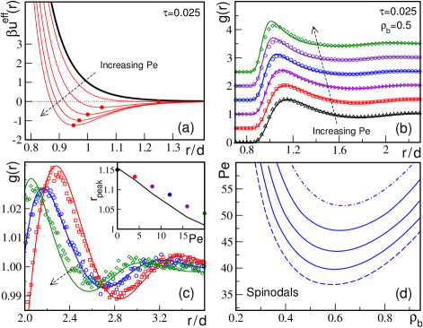
Figure 1: Activity induces effective attraction. Passive potential $\beta u(r)\!=\!r^{-12}\!$. (a) Increasing $Pe$ (in steps of $8$) from $0$ to $40$ generates an effective interparticle attraction. Points indicate the potential minima. (b) Radial distribution function, $g(r)$, from simulation (points) and theory (lines) for $\rho_{b}\!=\!0.5$ and $Pe\!=\!0$ to $20$ (in steps of $4$). Curves are shifted vertically for clarity. (c) As in (b), but focusing on larger separations for $Pe=4$ (squares), $12$ (circles) and $20$ (diamonds). Inset: position of the first peak in $g(r)$ as a function of $Pe$. (d) Spinodals for $\tau=0.045$ (dot-dashed) to $0.065$ (long dashed) in steps of $0.005$.

II Results

II.1 Motility-induced phase separation (MIPS)

To illustrate how activity can generate an effective attraction in a passively repulsive system we consider the non-specific potential $\beta u(r)=r^{-12}$. In Fig.1a we show the evolution of the effective potential (13) for fixed $\tau$ as a function of the dimensionless velocity $Pe\!=\!v_{0}d/D_{t}$. For $Pe\!\gtrsim\!10$ the effective potential develops an attractive tail. As $Pe$ is increased the potential well deepens, the minimum moves to smaller separations and the radius of the soft repulsive core decreases. These trends are consistent with the intuitive picture that persistent motion drives soft particles into one another (the soft core radius reduces) and that they remain dynamically coupled (‘trapped’) for longer than in the corresponding passive system. Within our equilibrium picture the trapping is accounted for by the effective attraction.

For systems at finite density the pair potential (13) is an approximation, because three- and higher-body interactions will play a role (see equation (8)). However, for simplicity we henceforth employ the pair potential (13) for all calculations, as we anticipate that this will provide the dominant contribution. Although corrections to this assumption can be made, they obscure the physical picture and come at the expense of a more complicated theory. The validity of the pair potential approximation is justified a posteriori by the comparison with simulation for the finite density pair correlations.

In Fig.1b we show the steady-state (isotropic) radial distribution function for $\rho_{b}\!=\!0.5$ for various values of $Pe$. We employ the effective pair potential (13) together with liquid state integral equation theory and compare theoretical predictions with direct Brownian dynamics simulation of equations (1) and (2). The integral equation theory we employ is the soft mean-spherical approximation (SMSA) proposed by Madden and Rice madden1980 . This approximate closure of the Ornstein-Zernike equation is known to provide reliable results for the pair stucture of Lennard-Jones type potentials. Given the form of the effective pair potential shown in Fig.1 the SMSA would seem to be a reasonable choice of closure. Details of the integral equation theory and the simulation procedure are given in Appendices C and D, respectively.

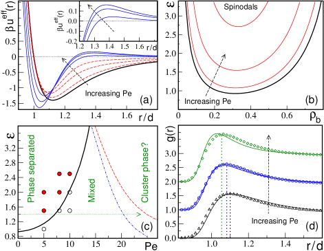
Figure 2: From active suppression of phase separation to a cluster phase. Passive potential $\beta u(r)\!=\!4\,\varepsilon(r^{-12}\!-r^{-6})$ with $\varepsilon\!=\!1.4$. (a) Effective potential (13) for $\tau\!=\!0.025$ and $Pe\!=\!0$ (black) $4,8,12$ (red broken lines) and $20,28,36$ (blue). Inset: zoom of the repulsive peak for $Pe\!=\!20,28,36$. (b) Spinodals for $Pe\!=\!0,4,8,12$. Increasing $Pe$ increases $\varepsilon_{\rm crit}$, the critical value of $\varepsilon$. (c) $\varepsilon_{\rm crit}$ as a function of $Pe$ (black full line) and the locus of points for which the repulsive peak of $\beta u^{\rm eff}$ takes the value $0.1$ (red dashed) and $0.05$ (blue dot-dashed). Open (closed) circles indicate points where BD simulation find a mixed (phase-separated) state (see figure 3). Arrow indicates path taken in (a). (d) Theory (lines) and simulation (symbols) data (shifted for clarity) for $g(r)$ at $\varepsilon=0.5$, $\rho_{b}=0.3$ for $Pe=0$ (black), $12$ (blue) and $20$ (green). Dotted lines indicate peak positions.

We find that as $Pe$ is increased the main peak of $g(r)$ grows in height and shifts to smaller separations (see inset to Fig.1c), reflecting the changes in the effective potential. In the main panel of Fig.1c we focus on the second and third peaks. The quantitative accuracy of the theory in describing the decay of $g(r)$ is quite striking, in particular the phase shift induced by increasing activity is very well described. Further comparison for other parameter values (not shown) suggests that (13) combined with the SMSA theory provides an accurate account of the asymptotic decay of pair correlations.

In Fig.1d we show the spinodal lines mapping the locus of points for which the static structure factor, $S(q)=(1-\rho_{b}c(q))^{-1}$, diverges at vanishing wavevector. Simulations have shown that MIPS is consistent with a spinodal instability fily2012 . As $\tau$ is decreased the critical point moves to higher values of $Pe$ and to slightly higher densities. When compared with the spinodal of a standard Lennard-Jones system (e.g. the black curve in Fig.2b) the critical points in Fig.1d lie at rather higher values of $\rho_{b}$. This suggests that typical coexisting liquid densities for MIPS will be larger than those found in equilibrium phase separated systems, as has been observed in simulation fily2012 ; redner2013 .

II.2 Suppression of phase separation

We next consider the influence of activity on a Lennard-Jones system, $\beta u(r)\!=\!4\varepsilon(r^{-12}\!-r^{-6})$. For a phase-separated passive system, recent experiments and simulations have demonstrated that increasing $Pe$ first suppresses the phase separation schwarz-linek2012 and then leads at higher $Pe$ to a reentrant MIPS redner2013 . Schwarz-Linek et al. have argued that the suppression of phase separation at lower to intermediate $Pe$ occurs in their system because particle pairs bound by the attractive (depletion) potential begin to actively escape the potential well, and that this can be mimicked using an effective potential less attractive and shorter-ranged than the bare potential schwarz-linek2012 .

To investigate these phenomena we set $\varepsilon\!=\!1.4$, which ensures a phase separated passive state barker_henderson1976 , and consider the evolution of the effective potential as a function of $Pe$. In Fig.2a we show that as $Pe$ is increased from zero to the value $18$ both the depth and range of the effective potential reduce significantly, consistent with the expectation of Schwarz-Linek et al. schwarz-linek2012 . Spinodals within this range of $Pe$ values, identifying where the static structure factor diverges at zero wavevector, are shown in Fig.2b. As $Pe$ is increased the critical point moves to higher values of $\varepsilon$ (cf. Figs.1 and 3 in Ref.schwarz-linek2012 ). A passively phase-separated system will thus revert to a single phase upon increasing the activity. To examine this behaviour in more detail we show in Fig.2c the trajectory of the critical point in the ($Pe,\varepsilon$) plane. Above the line there bulk densities for which phase separation occurs.

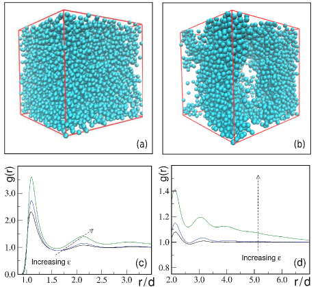
Figure 3: Simulated phase separation. (a) Snapshot of a mixed system at $t/\tau_{B}=40$, $Pe=8$, $\varepsilon/(k_{B}T)=1.5$. (b) Snapshot of a phase separating system at the same time and $Pe=8$, $\varepsilon=2.5$. (c) The radial distribution function, $g(r)$, for $\varepsilon=1.5$ (black curve), 2 (blue curve), and 2.5 (green curve). (d) As in (c) but focusing on larger distances. From the snapshots together with the long range behaviour of the $g(r)$ we can distinguish between a mixed and a phase separated system. The slow decay to the asymptotic value of unity, as shown in (d), indicates phase separation.

In order to test the predicted trajectory of the critical point we have performed Brownian dynamics simulations at a bulk density $\rho_{b}\!=\!0.4$, which lies close to the critical density barker_henderson1976 , for various values of $\varepsilon$ and the $Pe$ values $5,8$ and $10$. Visual inspection of the simulation snapshots reveals the existence of voids in the particle configurations corresponding to a phase separated state (see Figs.3a and 3b for snapshots). This visual impression can be made more quantitative by calculating the radial distribution function. Phase separating states generate a very characteristic slow decay of $g(r)$ (Figs.3c and 3d) which provides a useful indicator. The open circles in Fig.2c represent mixed states, whereas closed circles indicate phase separated statepoints. The phase boundary predicted by the theory is highly consistent with the simulation data.

II.3 Cluster phase

Returning to Fig.2a, we find that for $Pe\!>\!18$ the effective potential develops a repulsive barrier, which grows in height (see inset) with increasing $Pe$, while the potential minimum becomes deeper. It is well-known that potentials with a short-ranged attraction and long-ranged repulsion (SALR potentials) exhibit unusual equilibrium phase behaviour, including clustering and microphase-separation sear1997 ; archer2007 . Although the attractive component of the potential may favour phase separation, the long range repulsion destabilises distinct liquid and gas phases and causes them to break up into droplets or clusters. This represents a non-spinodal type of phase transition, characterized by a divergence in the structure factor at finite wavevector. The appearance of a repulsive barrier in the effective potential suggests that a similar mechanism may be at work in passively attractive systems subject to high $Pe$ activity.

In Fig.2c we show the locus of points where the effective potential peak height attains a given value (we choose $0.05$ and $0.1$ for illustration). When these ‘isorepulsion curves’ are viewed together with the critical point trajectory the resulting phase diagram is very similar to that obtained by Redner et al. in their simulation study of two-dimensional active Lennard-Jones particles (cf. figure 1 in Ref.redner2013 ). However, a detailed study of the connection between the potential barrier and high $Pe$ clustering goes beyond the scope of the present work.

III Discussion

In summary, we have shown that systems of active spherical Brownian particles can be mapped onto an equilibrium system interacting via an effective, activity-dependent many-body potential. The only required inputs are the bare potential, thermodynamic statepoint and the parameters specifying the state of activity. Our theory captures the phenomenon of MIPS in repulsive systems and provides first-principles predictions for the activity dependence of the pair correlations, in very good agreement with Brownian dynamics simulation. As far as we are aware there exists no other approach capable of predicting from the microscopic interactions the pair correlation functions of an active system. Further insight into the steady state particle distribution could in principle be obtained by investigating the three-body correlations. These could be obtained by employing the effective potential in a higher-order liquid state integral equation theory (see e.g. brader_triplet and references therein).

For passively attractive systems the theory rationalizes the experimental finding schwarz-linek2012 that increasing activity can suppress passive phase separation. We find that as $Pe$ is increased from zero to intermediate values the minimum of the effective potential becomes less deep, thus weakening the cohesion of the liquid phase. To the best of our knowledge there is currently no alternative theoretical explanation of phase-transition suppression in active suspensions. It is an appealing aspect of our theory that the suppression of passive phase separation follows naturally from the same approach which yields activity-induced attraction for repulsive potentials. For high values of $Pe$ the appearance of a repulsive barrier in the effective potential suggests that the reentrant phase separation observed in simulations redner2013 may be interpreted using concepts of equilibrium clustering in SALR potential systems. This will be a subject of future detailed investigations. It is known that care must be exercised when analysing SALR potentials, as traditional liquid state theories can prove misleading archer2007 .

A key step in our development is the Fox approximation fox1986 , which yields an effective Markovian description of the coarse-grained equation (3). Making a Markovian approximation automatically imposes an effective equilibrium, however, we are aware that there exist certain situations for which this breaks down cates2013 ; cates_tailleur2014 . Establishing more clearly the range of validity of our approach, as well as its possible extensions, will be the subject of ongoing study. However, it is already clear that going beyond the Markovian approximation will be very challenging. Indeed, such a step may not even be desirable. Any kind of non-Markovian description would lead inevitably to a loss of the effective equilibrium picture and the physical intuition associated with it. It thus seems likely that practical improvements to the present approach will retain the Markovian description while seeking to optimize, or improve upon, the Fox approximation for certain classes of bare potential. Very recently, Maggi et al. have employed an alternative approach to treating stochastic processes driven by Ornstein-Uhlenbeck noise maggi2015 . A comparison of their approach with the Fox method employed here would be very interesting.

With a view to further applications of our approach, we note that there has recently been considerable interest in active suspensions at very high densities faragebrader_arxiv ; ni2013 ; berthier2013 ; szamel_berthier2015 . In particular, it has been found using computer simulations that activity has a strong influence on the location of the hard-sphere glass transition, dynamic correlation functions, such as the intermediate scattering function, and static pair correlations ni2013 . Within our effective equilibrium framework, increasing the activity of a passively repulsive system generates an effective attraction. We can therefore anticipate that for volume fractions just above the glass transition it will be possible to observe a reentrant glass transition, namely a melting of the glass followed by revitrification, as a function of increasing $Pe$. Moreover, the nontrivial evolution of the effective potential as a function of $Pe$ for attractive bare potentials (cf. Fig.2a) suggests these systems will present a rich variety of glassy states. Work along these lines is in progress.

Finally, we mention that a natural generalization of the present theory is to treat spatially inhomogeneous systems in external fields. Recent microscopic studies of active particles under confinement (e.g. in a harmonic trap pototsky2012 ) have provided considerable insight, however none of the existing approaches have considered effective interparticle interactions. Inhomogeneous generalization of the present theory enables the interaction between MIPS and external fields to be investigated on the microscopic level. Our preliminary investigations reveal, for example, activity-induced wetting at a planar substrate and capillary-condensation under confinement. This will be presented in a future publication.

Appendix A Coarse-grained Langevin equation

Equation (2) describes the orientational diffusion of an active particle. The corresponding conditional probability distribution function $\Upsilon(\boldsymbol{p},t\,|\,\boldsymbol{p}_{0},t_{0})$, where $t>t_{0}$, obeys a Fokker-Planck equation which can be obtained by usual techniques gardiner ,

$$\frac{\partial}{\partial t}\Upsilon(\boldsymbol{p},t\,|\,\boldsymbol{p}_{0},t_{0})=D_{r}\boldsymbol{R}^{2}\Upsilon(\boldsymbol{p},t\,|\,\boldsymbol{p}_{0},t_{0})\,,$$ (14)

where $\boldsymbol{R}\equiv(\boldsymbol{p}\times\nabla_{\boldsymbol{p}})$ is the intrinsic angular momentum differential operator. Eq.(14) describes nothing but a diffusion process on the unit sphere. This problem is well-known when studying, e.g., dielectric relaxation in polar liquids debye1929 ; fatuzzo1967 ; zwanzig1970 ; berne1975 . In spherical coordinates, (14) becomes

$$\frac{1}{D_{r}}\frac{\partial}{\partial t}\Upsilon(\Omega,t\,|\,\Omega_{0},t_{0}) =\left[\frac{1}{\sin\vartheta}\frac{\partial}{\partial\vartheta}\left(\sin\vartheta\frac{\partial}{\partial\vartheta}\right)\right.$$

$$\phantom{=}\left.+\frac{1}{\sin^{2}\vartheta}\frac{\partial^{2}}{\partial\varphi^{2}}\right]\Upsilon(\Omega,t\,|\,\Omega_{0},t_{0}),$$ (15)

where we have defined $\Omega\equiv(\vartheta,\varphi)$.

Assuming that $\Upsilon$ and its derivatives are continuous on the sphere arfken2013 , we expand the probability distribution function $\Upsilon$ in spherical harmonics

$$\Upsilon(\Omega,t\,|\,\Omega_{0},t_{0})=\sum_{l=0}^{\infty}\sum_{m=-l}^{l}A_{lm}(t\,|\,\Omega_{0},t_{0})Y_{lm}(\Omega)\,,$$ (16)

where $Y_{lm}$ are the spherical harmonics and $A_{lm}$ are coefficients encoding the initial condition. We also recall that spherical harmonics are eigenvectors of the operator $\boldsymbol{R}^{2}$ (in spherical coordinates), namely that

$$\boldsymbol{R}^{2}Y_{lm}=-l(l+1)Y_{lm}\,.$$ (17)

Inserting (16) in (A) and using (17) we obtain

$$\sum_{l,m}\frac{\partial}{\partial t} A_{lm}(t\,|\,\Omega_{0},t_{0})Y_{lm}(\Omega)=$$

$$-D_{r}\sum_{l,m}l(l+1)A_{lm}(t\,|\,\Omega_{0},t_{0})Y_{lm}(\Omega).$$ (18)

Multiplying both sides of (A) by $Y_{l^{\prime}m^{\prime}}^{\ast}(\Omega)$, integrating over solid angle and using the orthogonality property, $\int d\Omega\,Y_{l^{\prime}m^{\prime}}^{*}(\Omega)Y_{lm}(\Omega)=\delta_{m,m^{\prime}}\delta_{l,l^{\prime}}$, yields

$$\frac{\partial}{\partial t}A_{lm}(t\,|\,\Omega_{0},t_{0})=-D_{r}l(l+1)A_{lm}(t\,|\,\Omega_{0},t_{0})\,,$$ (19)

which has the solution

$$A_{lm}(t\,|\,\Omega_{0},t_{0})=e^{-D_{r}l(l+1)(t-t_{0})}a_{lm}(\Omega_{0})\,,$$ (20)

where the $a_{lm}$ are a new set of coefficients. The probability distribution is thus given by

$$\Upsilon(\Omega,t\,|\,\Omega_{0},t_{0})=\sum_{l,m}e^{-D_{r}l(l+1)(t-t_{0})}a_{lm}(\Omega_{0})Y_{lm}(\Omega).$$ (21)

The initial condition,

$$\Upsilon(\Omega,t_{0}\,|\,\Omega_{0},t_{0})=\delta(\Omega-\Omega_{0})\,,$$ (22)

together with the completeness relation of the spherical harmonics,

$$\delta(\Omega-\Omega_{0})=\sum_{l=0}^{\infty}\sum_{m=-l}^{l}Y_{lm}(\Omega)Y_{lm}^{\ast}(\Omega_{0}),$$ (23)

allows the missing coefficients to be identified,

$$a_{lm}(\Omega_{0})=Y_{lm}^{\ast}(\Omega_{0})\,.$$ (24)

The conditional probability distribution is now fully determined as

$$\Upsilon(\Omega,t\,|\,\Omega_{0},t_{0})=\sum_{l=0}^{\infty}\sum_{m=-l}^{l}e^{-D_{r}l(l+1)(t-t_{0})}Y_{lm}^{\ast}(\Omega_{0})Y_{lm}(\Omega).$$ (25)

As $t\to\infty$ only the terms with $l=0$ survive. The steady-state distribution function is thus given by

$$\Upsilon_{eq}(\Omega)=\lim_{t\to\infty}\Upsilon(\Omega,t\,|\,\Omega_{0},t_{0})=(4\pi)^{-1}.$$ (26)

The conditional and equilibrium distributions, (25) and (26), respectively, can be used to coarse-grain the exact Langevin equations (1) and (2). The approach taken is to consider the orientation vector $\boldsymbol{p}_{i}(t)$ attached to particle $i$ as a stochastic variable and to provide its full statistical characterization. In spherical coordinates the orientation vector is given explicitly by

$$\boldsymbol{p}(t) =(p_{x}(t),p_{y}(t),p_{z}(t))^{T}$$

$$=(\cos\varphi(t)\sin\vartheta(t),\sin\varphi(t)\sin\vartheta(t),\cos\vartheta(t))^{T},$$ (27)

where $\varphi$ and $\vartheta$ are the azimuthal and polar angles respectively. Using (26) we have that

$$\langle p_{z}(t)\rangle =\int d\Omega\,\Upsilon_{eq}(\Omega)\cos\vartheta=0,$$ (28)

together with analagous results for the $x$ and $y$ components

$$\langle p_{x}(t)\rangle=0=\langle p_{y}(t)\rangle\,.$$ (29)

Defining the new stochastic variable by $\boldsymbol{\chi}_{i}(t)\equiv v_{0}\,\boldsymbol{p}_{i}(t)$, its first moment is thus given by

$$\langle\boldsymbol{\chi}_{i}(t)\rangle=v_{0}\langle\boldsymbol{p}_{i}(t)\rangle=\boldsymbol{0}.$$ (30)

Calculation of the equilibrium correlation matrix requires the conditional probability distribution function given by (25). For example, for the $zz$ component, we obtain

$$\langle p_{z}(t)p_{z}(t_{0})\rangle =\!\!\!\int\!\!d\Omega\!\!\int\!\!d\Omega_{0}\cos\vartheta\cos\vartheta_{0}\Upsilon(\Omega,t\,|\,\Omega_{0},t_{0})\Upsilon_{eq}(\Omega_{0})$$

$$=\frac{1}{3}\int d\Omega\int d\Omega_{0}\sum_{l,m}e^{-D_{r}l(l+1)(t-t_{0})}\times$$

$$\phantom{=}\times Y_{10}^{\ast}(\Omega)Y_{lm}(\Omega)Y_{10}(\Omega_{0})Y^{\ast}_{lm}(\Omega_{0})$$

$$=\frac{1}{3}e^{-2D_{r}|t-t_{0}|},$$ (31)

where we have expressed the cosine functions in terms of spherical harmonics, $Y_{10}=\sqrt{3/(4\pi)}\cos\vartheta=Y_{10}^{\ast}$, and used the orthogonality property. Calculations for the $xx$ and $yy$ components are performed in the same spirit. We thus obtain

$$\langle p_{x}(t)p_{x}(t_{0})\rangle=\frac{1}{3}e^{-2D_{r}|t-t_{0}|}=\langle p_{y}(t)p_{y}(t_{0})\rangle,$$ (32)

whereas off-diagonal components of the correlation matrix are all zero. We can thus conclude that

$$\langle\boldsymbol{\chi}_{i}(t)\boldsymbol{\chi}_{j}(t^{\prime})\rangle=v_{0}^{2}\langle\boldsymbol{p}_{i}(t)\boldsymbol{p}_{j}(t^{\prime})\rangle=\frac{v_{0}^{2}}{3}e^{-2D_{r}|t-t^{\prime}|}\boldsymbol{1}\delta_{ij}.$$ (33)

It has been shown ghosh2012 that the probability distribution function (25) can be well approximated by an expression which generalizes the planar Gaussian function to the sphere. The new noise function $\boldsymbol{\chi}_{i}(t)$ is thus approximately Gaussian distributed with zero mean and exponentially decaying correlations. The coarse-grained Langevin equation (3) thus describes a stochastic process with additive colored-noise.

Appendix B Approximate Fokker-Planck equation

To derive from (3) an approximate Fokker-Planck equation we apply the functional calculus methods of Fox fox1986 . We address the one-dimensional case before generalizing to higher dimension. Consider the stochastic differential equation

$$\dot{x}(t)=F(x)+g(x)\chi(t)\,,$$ (34)

where $F(x)$ and $g(x)$ may be nonlinear functions in $x$. If $g(x)=1$, the process is then called additive, otherwise it is called multiplicative. The noise function $\chi(t)$ is by definition Gaussian distributed with zero mean. Its second moment determines whether it is a white or colored noise. As we are interested here in the case of additive colored noise we set $g(x)=1$.

In the framework of functional calculus, the Gaussian nature of $\chi(t)$ is expressed by the following probability distribution functional,

$$P[\chi]=Ne^{-\frac{1}{2}\int ds\int ds^{\prime}\chi(s)\chi(s^{\prime})K(s-s^{\prime})}\,,$$ (35)

where the function $K$ is the inverse of the $\chi$ correlation function and the normalization constant is expressed by a path integral over $\chi$,

$$N^{-1}=\int D[\chi]e^{-\frac{1}{2}\int ds\int ds^{\prime}\chi(s)\chi(s^{\prime})K(s-s^{\prime})}\,.$$ (36)

The first and second moments of $\chi$ are given by

$$\langle\chi(t)\rangle =0\,,$$ (37)

$$\langle\chi(t)\chi(s)\rangle =C(t-s)\,.$$ (38)

Recalling that the functional derivative may be defined according to

$$\frac{\delta I[\phi]}{\delta\phi(t^{\prime})}=\left.\frac{d}{d\lambda}I[\phi(t)+\lambda\delta(t-t^{\prime})]\right|_{\lambda=0}\,,$$ (39)

we now derive two useful identities. The first concerns the functional derivative of the probability distribution functional,

$$\frac{\delta P[\chi]}{\delta\chi(t)} =\frac{\delta N}{\delta\chi(t)}e^{-\frac{1}{2}\int ds\int ds^{\prime}\chi(s)\chi(s^{\prime})K(s-s^{\prime})}$$

$$\phantom{=}+N\frac{\delta}{\delta\chi(t)}e^{-\frac{1}{2}\int ds\int ds^{\prime}\chi(s)\chi(s^{\prime})K(s-s^{\prime})}$$

$$=-P[\chi]\int dsK(t-s)\chi(s)\,,$$ (40)

where, using (39) and (37), it can be easily shown that $\delta N/\delta\chi(t)=0$. The second identity demonstrates the inverse relation between the functions $K$ and $C$. The second functional derivative of $P[\chi]$ yields

$$\frac{\delta^{2}P[\chi]}{\delta\chi(t^{\prime})\delta\chi(t)} =P[\chi]\left\{\!\int\!\!ds^{\prime}\!\!\!\int\!\!dsK(t^{\prime}-s^{\prime})K(t-s)\chi(s^{\prime})\chi(s)\right.$$

$$\phantom{=}\left.\phantom{\int}\!\!-K(t-t^{\prime})\right\}\,,$$ (41)

where use of (40) has been made. Using (B) and (38) together with the normalization $\int D[\chi]P[\chi]=1$, leads to

$$0 =\int D[\chi]\frac{\delta^{2}P[\chi]}{\delta\chi(t^{\prime})\delta\chi(t)}$$

$$=\int\!\!ds^{\prime}K(t^{\prime}-s^{\prime})\int\!\!dsK(t-s)C(s-s^{\prime})-K(t-t^{\prime})\,,$$ (42)

which implies that

$$\int\!\!dsK(t-s)C(s-s^{\prime})=\delta(t-s^{\prime})\,.$$ (43)

The solution to the stochastic process described by (34), namely the probability distribution functional for $x(t)$, is given by the formal expression

$$P(y,t)=\int D[\chi]P[\chi]\delta(y-x(t))\,.$$ (44)

Taking the time derivative of (44) yields

$$\frac{\partial}{\partial t}P(y,t) =-\frac{\partial}{\partial y}[F(y)P(y,t)]$$

$$\phantom{=}-\frac{\partial}{\partial y}\int D[\chi]\delta(y-x(t))P[\chi]\,\chi(t)\,.$$ (45)

The product $P[\chi]\,\chi(t)$ appearing in the second term can be rewritten in the following way

$$P[\chi]\,\chi(t) =P[\chi]\int ds\delta(t-s)\chi(s)$$

$$=-\int ds^{\prime}C(t-s^{\prime})\frac{\delta P[\chi]}{\delta\chi(s^{\prime})}\,,$$ (46)

where we have used (43) and (40). Inserting (B) back into the second term of (B) and integrating by parts gives us

$$\int D[\chi]\delta(y-x(t))P[\chi]\chi(t)$$

$$=-\int\!\!ds^{\prime}C(t-s^{\prime})\!\!\int\!\!D[\chi]\left(\frac{\partial}{\partial y}\delta(y-x(t))\right)\frac{\delta x(t)}{\delta\chi(s^{\prime})}P[\chi],$$ (47)

which serves as the exact starting point for Fox’s approximation scheme fox1986 .

In order to progress further we need to calculate $\delta x(t)/\delta\chi(s^{\prime})$. Applying the functional derivative with respect to $\chi(t^{\prime})$ on (34) yields a first-order differential equation,

$$\frac{d}{dt}\frac{\delta x(t)}{\delta\chi(t^{\prime})} =\frac{\delta\dot{x}(t)}{\delta\chi(t^{\prime})}=F^{\prime}(x)\frac{\delta x(t)}{\delta\chi(t^{\prime})}+\delta(t-t^{\prime})\,,$$ (48)

the solution of which is

$$\frac{\delta x(t)}{\delta\chi(s^{\prime})} =\int_{0}^{t}\!\!\!ds\,e^{\int_{s}^{t}d\tilde{s}F^{\prime}(x(\tilde{s}))}\delta(s-s^{\prime})$$

$$=e^{\int_{s^{\prime}}^{t}dsF^{\prime}(x(s))}\Theta(t-s^{\prime})\,,$$ (49)

where $\Theta$ is the Heaviside step function, which we define here as follows

$$\Theta(t-s^{\prime})=\left\{\begin{array}[]{ll}1,&t>s^{\prime}\\ \frac{1}{2},&t=s^{\prime}\\ 0,&t<s^{\prime}\,.\end{array}\right.$$

Using (B) in (B) we can rewrite (B) in an alternative form

$$\frac{\partial}{\partial t}P(y,t)=-\frac{\partial}{\partial y}[F(y)P(y,t)]$$

$$+\frac{\partial^{2}}{\partial y^{2}}\!\!\left\{\!\int_{0}^{t}\!\!\!\!ds^{\prime}C(t-s^{\prime})\!\!\!\int\!\!\!D[\chi]P[\chi]e^{\int_{s^{\prime}}^{t}dsF^{\prime}(x(s))}\delta(y-x(t))\!\!\right\},$$ (50)

which already begins to resemble a Fokker-Planck-type equation. However, because of the non-Markovian nature of $\int_{s^{\prime}}^{t}dsF^{\prime}(x(s))$ appearing in the exponential of (B), it is apparent that a reduction of this term to an expression containing $P(y,t)$ is not possible. An approximation is required.

The colored noise of interest here is characterized by an exponentially decaying correlation function (30). In the literature on non-Markovian processes the time-correlation functions are generally notated as follows

$$C(t-s)=\frac{D}{\tau}e^{-\frac{|t-s|}{\tau}}\,,$$ (51)

with a diffusion coefficient $D$ and a correlation time $\tau$. In order to retain some coherence with the existing literature we will here employ the standard notation of (51) and only use the relation of the parameters in (51) to those of (33) at the end of the calculation.

Returning to (B), we first perform a change of variable, $t^{\prime}\equiv t-s^{\prime}$, in the time-integral,

$$\int_{0}^{t}ds^{\prime}C(t-s^{\prime})e^{\int_{s^{\prime}}^{t}dsF^{\prime}(x(s))}=\int_{0}^{t}dt^{\prime}C(t^{\prime})e^{\int_{t-t^{\prime}}^{t}dsF^{\prime}(x(s))},$$ (52)

and then expand the time integral over $F^{\prime}$ in terms of $t^{\prime}$,

$$\int_{t-t^{\prime}}^{t}dsF^{\prime}(x(s))\approx F^{\prime}(x(t))t^{\prime}-F^{\prime\prime}(x(t))\dot{x}(t)\frac{t^{\prime 2}}{2}.$$ (53)

Neglecting the $t^{\prime 2}$ term in (53) enables the integral in (52) to be evaluated

$$\int_{0}^{t}ds^{\prime}C(t-s^{\prime})e^{\int_{s^{\prime}}^{t}dsF^{\prime}(x(s))}\approx\int_{0}^{t}dt^{\prime}C(t^{\prime})e^{F^{\prime}(x(t))t^{\prime}}$$

$$=\frac{D}{\tau}\int_{0}^{t}dt^{\prime}e^{-t^{\prime}(-F^{\prime}(x(t))+\frac{1}{\tau})}\approx\frac{D}{1-\tau F^{\prime}(x(t))}\,,$$ (54)

where we used (51), and the second approximation results from assuming a sufficiently large $t$. We can finally put (B) back into (B) to obtain an approximate Fokker-Planck equation,

$$\frac{\partial}{\partial t}P(y,t) \!=\!-\frac{\partial}{\partial y}[F(y)P(y,t)]+\!D\frac{\partial^{2}}{\partial y^{2}}\!\!\left(\!\frac{1}{1-\tau F^{\prime}(y)}P(y,t)\!\right).$$ (55)

This is Fox’s result for the approximate Fokker-Planck equation corresponding to the non-Markovian process (34). Eq.(55) implicity defines a Markovian process, which approximates the non-Markovian process of physical interest. However, the question of whether this represents the best approximation remains a subject of debate. We note that equation (55) has also been derived by Grigolini et al. faetti1988 using alternative methods which do not make any assumptions of a short correlation time.

The one-dimensional Fokker-Planck equation (55) can be generalized without much difficulty to describe a three-dimensional system of $N$ particles. The dynamics of interest is described by the stochastic equation (3). We now adapt the standard notation used above to that employed in the main text, namely $P(y,t)\rightarrow\Psi(\boldsymbol{r}^{N},t)$, $\tau\rightarrow\tau_{p}=1/(2D_{r})$ and $D\rightarrow v_{0}^{2}/3$, and recall that $D_{a}=v_{0}^{2}/(6D_{r})$ and $\zeta^{-1}=\beta D_{t}$ for the friction coefficient in (3). Making the appropriate replacements enables us to write the three-dimensional generalization of (55)

$$\frac{\partial}{\partial t} \Psi(\boldsymbol{r}^{N},t)=-\sum_{i=1}^{N}\nabla_{i}\cdot D_{t}\left[\beta\boldsymbol{F}_{i}(\boldsymbol{r}^{N})-\nabla_{i}\right]\Psi(\boldsymbol{r}^{N},t)$$

$$-\sum_{i=1}^{N}\nabla_{i}\cdot\left[-D_{a}\nabla_{i}\left(\frac{1}{1-\frac{D_{0}\nabla_{i}\cdot\beta\boldsymbol{F}_{i}(\boldsymbol{r}^{N})}{2D_{r}}}\Psi(\boldsymbol{r}^{N},t)\right)\right].$$ (56)

A simple rearrangement of terms in (B) leads directly to equations (5)-(8) in the main text.

Appendix C Integral equation theory

To calculate the steady-state radial distribution function, $g(r)$, from the effective pair potential (13) we employ an equilibrium liquid state integral equation developed by Madden and Rice madden1980 . This soft mean-spherical approximation (SMSA) exploits the Weeks-Chandler-Anderson splitting of the pair potential WCA into attractive and repulsive contributions, $u(r)=u_{\rm rep}(r)+u_{\rm att}(r)$, where the repulsive part is given by

$$u_{\rm rep}(r)=\begin{cases}u(r)-u(r_{\rm min})&\;\;\;\;r<r_{\rm min}\\ 0&\;\;\;\;r>r_{\rm min}\end{cases}$$ (57)

and the attractive part is given by

$$u_{\rm att}(r)=\begin{cases}u(r)&\;\;\;\;r>r_{\rm min}\\ u(r_{\rm min})&\;\;\;\;r<r_{\rm min}\end{cases}$$ (58)

where $r_{\rm min}$ is the position of the potential minimum. The total correlation function, $h(r)=g(r)-1$, is related to the shorter range direct correlation function, $c(r)$, by the Ornstein-Zernike equation hansen_mcdonald1986

$$h(r)=c(r)+\rho_{b}\int d{\boldsymbol{r}}^{\prime}h(|\boldsymbol{r}-\boldsymbol{r}^{\prime}|)c(r^{\prime}).$$ (59)

The SMSA approximation is given by the closure relation

$$c(r)=(1-e^{\beta u_{\rm rep}(r)})g(r)-\beta u_{\rm att}(r).$$ (60)

For the Lennard-Jones potential the closure relation (60) has been shown to provide results for $g(r)$ which are superior to both Percus-Yevick (PY) and Hypernetted Chain (HNC) theories madden1980 . Moreover, the SMSA theory predicts a true spinodal line in the parameter space, namely a locus of points for which the static structure factor, $S(k)=(1-\rho_{b}\tilde{c}(k))^{-1}$, diverges at vanishing wavevector. This behaviour is a consequence of the assumed asymptotic form of the direct correlation function, $c(r)\sim-\beta u_{\rm att}(r)$. Other standard integral equation theories, such as PY and HNC, do not exhibit a complete spinodal line, but rather a region within which the theory breaks down (‘no solutions region’) braderIJTP .

Appendix D Brownian Dynamics Simulations

In order to benchmark our theoretical predictions we perform Brownian dynamics simulations of $N$ particles, randomly initialized without overlap. The system is confined to a periodic cubic box, the size of which is determined by the number density according to $L^{3}=N/\rho_{b}$, where $L$ is the side length. The Langevin equations of motion, (1) and (2), are integrated via a standard Brownian dynamics scheme allen_tildesley with a constant time step of $\delta t/\tau_{B}=10^{-5}$.​ Both the translational and rotational noise are Gaussian random variables with a standard deviation of $\sigma_{t}\!=\!(2D_{0}T)^{\frac{1}{2}}$ and $\sigma_{r}\!=\!(2D_{r}T)^{\frac{1}{2}}$, respectively.

For the soft repulsive potential to be considered in this work, $\beta u(r)=r^{-12}$, we employ $N\!=\!2000$ particles. The potential is truncated and shifted at $r_{\rm cut}/d=2$. To provide good statistics for the static quantities the simulations are carried out for $10^{6}$ time steps, sampling every 1000 steps, which is equivalent to a total run time of $t_{\rm tot}/\tau_{B}=10$ and a sampling rate of $\tau_{B}/t_{sample}=100$. For the second system we will consider, the Lennard-Jones system, $\beta u(r)\!=\!4\epsilon(r^{-12}\!-r^{-6})$, we simulate a larger system of 5000 particles. The integration time of the equations of motion is the same as in the repulsive system, as is the cut-off radius. In this case, the runtime is $10^{7}$ and the particle positions are sampled every $10^{4}$ steps.

References

- (1) J. Palacci, C. Cottin-Bizonne, C. Ybert, and L. Bocquet Phys.Rev.Lett. 105 088304 (2010).
- (2) A. Erbe, M. Zientara, L. Baraban, C. Kreidler and P. Leiderer, J.Phys.:Condens.Matt. 20 404215 (2008).
- (3) J. Howse, R.A.L. Jones, A.J. Ryan, T. Gough, R. Vafabakhsh, and R. Golestanian, Phys.Rev.Lett. 99 048102 (2007).
- (4) R. Dreyfus, J. Baudry, M.L. Roper, M. Fermigier, H.A. Stone and J. Bibette, Nature 437 862 (2005).
- (5) J. Palacci, S. Sacanna1, A.P. Steinberg, D.J. Pine and P.M. Chaikin, Science 339 936 (2013).
- (6) T. Vicsek and A. Zafieris, Physics Reports 517 71 (2012).
- (7) S. Ramaswamy, Annual Review of Condensed Matter Physics 1 323 (2010).
- (8) P. Romanczuk, M. Bär, W. Ebeling, B. Lindner, and L. Schimansky-Geier, Eur.Phys.J. Special Topics 202 1 (2012)
- (9) M. E. Cates, Rep.Prog.Phys. 75 042601 (2012).
- (10) M. E. Cates and J. Tailleur, Annual Review of Condensed Matter Physics, 6 219 (2015).
- (11) J. Tailleur and M. E. Cates, Phys.Rev.Lett. 100 218103 (2008).
- (12) Y. Fily and M. C. Marchetti, Phys.Rev.Lett. 108 235702 (2012).
- (13) J. Stenhammar, A. Tiribocchi, R.J. Allen, D. Marenduzzo and M.E. Cates, Phys.Rev.Lett. 111 145702 (2013).
- (14) G. S. Redner, A. Baskaran and M. F. Hagan, Phys.Rev.E 88 012305 (2013).
- (15) D. Levis and L. Berthier, Phys.Rev.E 89 062301 (2014).
- (16) J. Schwarz-Linek et al., Proceedings of the National Academy of Sciences (USA) 109 4052 (2012).
- (17) F. Ginot, I. Theurkauff, D. Levis, C. Ybert, L. Bocquet, L. Berthier and C. Cottin-Bizonne, Phys.Rev.X 5, 011004 (2014).
- (18) A. Wysocki and R.G. Winkler and G. Gompper, EPL 105 48004 (2014).
- (19) M. E. Cates and J. Tailleur, EPL 101 20010 (2013).
- (20) J. Bialké, H. Löwen and T. Speck, EPL 103 30008 (2013).
- (21) A. P. Solon, Y. Fily, A. Baskaran, M. E. Cates, Y. Kafri, M. Kardar and J. Tailleur, arXiv:1412.3952 (2014).
- (22) S.C. Takatori, W. Yan, and J.F. Brady, Phys.Rev.Lett. 113 028103 (2014).
- (23) J. Stenhammar, D. Marenduzzo, R.J. Allen and M.E. Cates, Soft Matter 10 1489 (2014).
- (24) N. G. van Kampen, Physics Reports 24: 171 (1976).
- (25) N. G. van Kampen, Brazilian Journal of Physics 28 90 (1998).
- (26) S. Faetti, L. Fronzoni, P. Grigolini and R. Mannella, J.Stat.Phys. 52 951 (1988).
- (27) R. F. Fox, Phys.Rev.A 33 467 (1986).
- (28) R. F. Fox, Phys.Rev.A 34 4525(R) (1986).
- (29) A. Pototsky and H. Stark, EPL 98 50004 (2012).
- (30) W. Madden and S. Rice, J.Chem.Phys. 72 4208 (1980).
- (31) Useful tables of simulation data are to be found in: J. Barker and D. H. Henderson, Reviews of Modern Physics 48 587 (1976).
- (32) R. Sear and W. Gelbart, J.Chem.Phys. 110: 4582 (1997).
- (33) A. J. Archer and N. Wilding, Phys.Rev.E 76: 031501 (2007).
- (34) J.M. Brader, J.Chem.Phys. 128 104503 (2008).
- (35) C. Maggi, U.M.B. Marconi, N. Gnan and R. Di Leonardo, arXiv:1503.03123v2
- (36) T.F.F. Farage and J.M. Brader, Arxiv: 1403.0928
- (37) R. Ni, M.A. Cohen Stuart and M. Dijkstra, Nature Communications 4 2704 (2013).
- (38) L. Berthier and J. Kurchan, Nature Physics 9 310 (2013).
- (39) G. Szamel, E. Flenner and L. Berthier, Arxiv: 1501.01333
- (40) C. Gardiner, Handbook of stochastic methods (Springer, Berlin, 1985).
- (41) P. Debye Polar Molecules, (The Chemical Catalog Com- pany, Inc., 1929).
- (42) E. Fatuzzo and P.R. Mason, Proc. Phys. Soc. 90 741 (1967).
- (43) T.-W. Nee and R. Zwanzig, J. Chem. Phys. 52 6353 (1970).
- (44) B.J. Berne, J. Chem. Phys. 62 1154 (1975).
- (45) G.B. Arfken, H.J. Weber, and F.A. Harris, Mathematical Methods for Physicists (Elsevier, 2013).
- (46) A. Ghosh, J. Samuel, and S. Sinha, EPL 98 30003 (2012).
- (47) J. Weeks and D. Chandler and H. Anderson, J.Chem.Phys. 54 5237 (1971).
- (48) J.-P. Hansen and I. R. McDonald, Theory of simple liquids (Academic press, London, 1986).
- (49) J.M. Brader, International Journal of Thermophysics 27 394 (2006).
- (50) M. P. Allen and D. J. Tildesley (1991) Computer Simulation of Liquids (Oxford University Press, 1991).