Inspiraling black-hole binary spacetimes: Challenges in transitioning from analytical to numerical techniques

Abstract

We explore how a recently developed analytical black-hole binary spacetime can be extended using numerical simulations to go beyond the slow-inspiral phase. The analytic spacetime solves the Einstein field equations approximately, with the approximation error becoming progressively smaller the more separated the binary. To continue the spacetime beyond the slow-inspiral phase, we need to transition. Such a transition was previously explored at smaller separations. Here, we perform this transition at a separation of $D=20M$ (large enough that the analytical metric is expected to be accurate), and evolve for six orbits. We find that small constraint violations can have large dynamical effects, but these can be removed by using a constraint-damping system like the conformal covariant formulation of the Z4 system. We find agreement between the subsequent numerical spacetime and the predictions of post-Newtonian theory for the waveform and inspiral rate that is within the post-Newtonian truncation error.

I Introduction

The field of numerical relativity (NR) has progressed at a remarkable rate since the breakthroughs of 2005 Pretorius (2005); Campanelli et al. (2006a); Baker et al. (2006), when it first became possible to simulate the late inspiral, plunge, merger, and ringdown of black-hole binaries (BHBs). Recently, Lousto and Healy Lousto and Healy (2015) completed a long-term 50-orbit precessing BHB simulation using the moving punctures approach, and Szilagyi et al. Szilagyi et al. (2015) completed the longest BHB simulation to date: the last 176 orbits for a nonspinning, intermediate-mass-ratio ($m_{1}/m_{2}=1/7$) BHB using the generalized harmonic approach. This is a remarkable achievement, but the scaling of the inspiral time with the initial separation $T\sim D^{4}$ means that evolving a binary through the long inspiral is prohibitively expensive, even for highly efficient codes. Such a simulation becomes even more expensive when one is interested in performing long-term dynamical evolutions of the relativistic magnetohydrodynamics (MHD) of circumbinary disks around inspiraling supermassive BHBs (SMBHBs). This is because the circumbinary gas can exhibit significant secular variations on the time scale of hundreds to thousands of binary orbits.

In order to make these long-term simulations possible, our group developed a complementary approach to treat dynamical BHB spacetimes. In a series of papers Noble et al. (2012); Gallouin et al. (2012); Mundim et al. (2014); Zilhao et al. (2015); Zilhao and Noble (2014), we used an analytic spacetime that is an approximate solution to the Einstein field equations in the inspiral regime to describe the evolution of the accretion disks surrounding the binary and each of the individual BHs.

Our initial approach Noble et al. (2012), was one in which relativistic effects were present but relatively small. In the situation when gravity is weak [$r_{g}/r=GM/(rc^{2})\ll 1$] and motions are slow [$(v/c)^{2}\ll 1$], the post-Newtonian (PN) approximation gives a very good description of spacetime. One can then simply construct a PN metric which takes energy loss from the binary into account, accurately modeling both the mass loss and inspiral of the binary Blanchet (2014). Using a spacetime accurate to 2.5PN order [i.e., including terms up to $\sim(r_{g}/r)^{5/2}$], but describing the binary orbital evolution to 3.5PN, we demonstrated that circumbinary disks can track the inspiral of a SMBHB until the binary practically reaches the relativistic merger regime Noble et al. (2012). The shortcoming of this approach was that the PN metric was not valid very close to the BHs, and consequently, we excised any material that fell within 1.5 binary separations. This prevented us from studying the dynamics of the gas all the way down through the horizons of each BH.

In a more recent paper Mundim et al. (2014), we extended the metric to cover the full BHB spacetime up to the rapid plunge state. We did this by extending the framework established in Refs. Yunes et al. (2006); Yunes and Tichy (2006); Johnson-McDaniel et al. (2009) for constructing a spacetime metric valid for initial data, i.e., a metric accurate for all spatial points but in a very small time interval, to develop a metric valid for arbitrary times. In this approach, the near zone (NZ), i.e., a zone well outside the two BHs, but less than a gravitational wavelength from the binary, is still described using a PN expansion. In the far zone (FZ), i.e., farther than one wavelength from the binary, the metric is described by a post-Minkowskian (PM) expansion. Finally, near each BH, i.e., in the inner zone (IZ), the metric is described using a perturbed Kerr (here Schwarzschild) BH. The metrics covering the different zones are smoothly stitched together using asymptotic expansions and transition functions in their overlapping regions of validity.

This approach allows us to follow inspiraling SMBHBs over hundreds to thousands of binary orbits, the timescale on which gas accumulates, without having to solve the Einstein equations numerically. The numerical advantage here is that the numerical time step is limited by fluid characteristic speeds, rather than the much faster speed of light (this advantage is diminished if we want to evolve gas right near the horizons).

Here, we explore the possibility of using a hybrid approach; i.e., use the analytic metric for the long inspiral down to separations where our global spacetime metric is still valid, and then transition to a full numerical simulation using the analytic spacetime as initial data (the use of PN techniques to generate initial data for BHBs was first developed in Refs. Tichy et al. (2003); Kelly et al. (2007, 2010); Johnson-McDaniel et al. (2009); Mundim et al. (2011)). The way to do this is to convert our approximate spacetime prescription into suitable initial data for $3+1$ NR evolutions, evolve the data forward in time, and compare the orbital evolution, test particle trajectories, and gravitational radiation output with our approximate solution.

Perhaps more well known is the complimentary approach of combining PN and other analytical techniques with numerical waveforms to generate highly accurate hybrid waveforms. Many authors have explored this and, we refer the reader to Refs. Aasi et al. (2014); Ajith et al. (2012); Boyle et al. (2008); Buonanno et al. (2007, 2009); Campanelli et al. (2009); Nakano et al. (2011); Pan et al. (2010, 2011, 2014); Szilagyi et al. (2015); Taracchini et al. (2012, 2014) and references therein.

The main motivation of this paper is to develop techniques to smoothly transition from an analytically evolved spacetime to a numerically evolved one. By smooth, here we mean that all families of geodesics passing through the transition region will have continuous second derivatives. Here we are considering test particle trajectories as stand-ins for fluid trajectories. In particular, if there is a jump in the second derivative of the fluid, we can expect a quasiequilibrium fluid configuration to shock and therefore require a reequilibration that may take longer than the inspiral time. Of course, bulk binary dynamics are important too. Therefore, we want the physics of the inspiral (rate, orbital frequency) to be as unaffected by the transition as possible.

We note that the use of PN techniques to generate consistent initial data (i.e., data with the correct radiation content) provides the final ingredient proposed in the “Lazarus approach” to generating waveforms Baker et al. (2002); Campanelli et al. (2006b). The proposal there was to transition from PN to NR techniques and then from NR to perturbative techniques.

When using the global analytic metric as initial data, the resulting initial data are essentially equivalent (there is only a small difference in the NZ/FZ transition function and the two metric prescriptions coincide at $t=0$) to the initial data proposed in Johnson-McDaniel et al. Johnson-McDaniel et al. (2009) and first evolved in Reifenberger and Tichy Reifenberger and Tichy (2012). Reifenberger and Tichy compared evolutions of Bowen-York data Bowen and York (1980) to several different analytic initial data constructions, including Johnson-McDaniel et al.. Our work here extends upon the work of Reifenberger and Tichy in several ways. (i) We use the full 4-dimensional metric of Mundim et al. (2014) to compare the dynamics of the numerically evolved metric with the analytic one, (ii) we evolve binaries with separations large enough that the PN metric and binary dynamics are expected to be accurate, and (iii) we find techniques to ameliorate the inaccuracies associated with evolving these data that were discovered by Reifenberger and Tichy. These inaccuracies arise both from constraint violations, due to the fact that our global metric solves the Einstein field equations only approximately, and from inaccuracy in the PN orbital angular momentum and inspiral rate, which can lead to eccentricity in the numerical binary evolution.

For the current work, we start the full numerical simulations when the binary is separated by $D=20M$ and evolve for six orbits. As shown in Ref. Lousto and Zlochower (2013), where the authors there explored numerical simulations of Bowen-York data at separations ranging from $D=100M$ to $D=20M$, there is good agreement between the predictions of PN theory and numerical simulations at $D=20M$. Additionally, simulations starting at $D=20M$ down to merger are possible with our current codes, as demonstrated in Ref. Lousto and Healy (2015) (such a simulation would require approximately 1 $10^{6}$ CPU hours on an AMD Opteron machine).

This paper is organized as follows: In Sec. II, we review how the analytic BHB inspiral metric is constructed, as well as how it is used to generate $3+1$ initial data. In Sec. III, we describe the techniques we used to numerically evolve the spacetime metric. In Sec. IV, we provide details on how the simulations were performed and the key outcomes of these simulations. In Sec. V, we compare the results from the numerical simulation at separations $\sim 20M$ with the predictions of PN theory. Finally, in Sec. VI we discuss our results both in terms of the accuracy of the binary dynamics (e.g., inspiral rate and orbital frequency) and in terms of gravitational waveform generation.

Throughout this paper, we use the geometric unit system, where $G=c=1$, with the useful conversion factor $1M_{\odot}=1.477\;{\rm{km}}=4.926\times 10^{-6}\;{\rm{s}}$.

II analytic BHB inspiral metric

In this paper, we restrict our analysis to non-spinning BHs in quasicircular orbits. In this context, it is useful to provide a brief review here of our approximate solution to the Einstein field equations of a BHB spacetime in the inspiral regime Mundim et al. (2014). The inclusion of spins, both aligned Gallouin et al. (2012) and unaligned in this spacetime framework will be the subject of future studies.

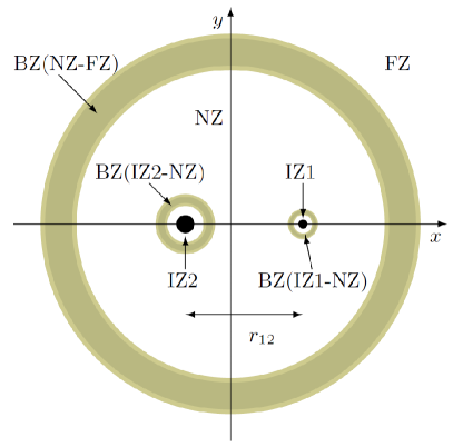
Figure 1: Schematic diagram of the zones. BH1 and BH2 are denoted by solid black dots, where the orbital separation is $r_{12}$. The BZs are denoted with gray shells, the outer one representing the FZ/NZ BZ and the two inner ones representing the NZ/IZ BZs (see also Table 1). The IZ, NZ and FZ are also shown in the figure.

Table 1: Location of the inner, near, and far zones, as well as the buffer zones joining them. Here $r_{\rm in}$ and $r_{\rm out}$ are the approximate inner and outer boundaries of a given zone, $m_{i}$ is the mass of BH $i$, $r_{i}$ is the coordinate distance to BH $i$, $r_{12}$ is the binary separation, and $\lambda$ is the wavelength of gravitational radiation emitted by the binary.

Zone	$r_{\rm in}$	$r_{\rm out}$	Region
IZ BH1 ($r_{1}$)	$0$	$\ll r_{12}$	$\cdot$
IZ BH2 ($r_{2}$)	$0$	$\ll r_{12}$	$\cdot$
NZ ($r_{A}$)	$\gg m_{A}$	$\ll\lambda$	$\cdot$
FZ ($r$)	$\gg r_{12}$	$\infty$	$\cdot$
IZ-NZ BZ	$\cdot$	$\cdot$	$m_{A}\ll r_{A}\ll r_{12}$
NZ-FZ BZ	$\cdot$	$\cdot$	$r_{12}\ll r\ll\lambda$

This framework was first introduced in Refs. Yunes et al. (2006); Yunes and Tichy (2006); Johnson-McDaniel et al. (2009) as initial data for BHB evolutions, and was generalized in Ref. Mundim et al. (2014) to be a full BHB spacetime. In this framework, the spacetime is constructed by asymptotically matching metrics in three different zones characterizing three different spacetime regions of validity for different analytic metrics: (i) a far zone (FZ) where the spacetime can be described by a two-body perturbed flat spacetime with outgoing gravitational radiation and where retardation effects are fully accounted for; (ii) a near zone (NZ) which is less than one GW length from the center of mass of the binary (but not too close to each BH) that is described by a PN metric (this includes retardation effects at a perturbative level and binding interactions between the two BHs); and (iii) inner zones (IZs) that are described by perturbed Schwarzschild (or Kerr) BHs. The full spacetime is then constructed by smoothly transitioning from zone to zone in the so-called buffer zones (BZs). A schematic diagram of these zones and a table describing where the zone boundaries are located are provided in Fig. 1 and Table 1 (these were also presented in Refs. Gallouin et al. (2012); Mundim et al. (2014)).

In the sections below, we will refer to these initial data as the second-order analytical metric. It is constructed by asymptotically matching a 2.5PN metric in the NZ [the matching is only done for terms up through ${\cal O}(v/c)^{4}$] to a Schwarzschild metric with quadrupole (and its time derivatives) and octupole tidal deformations in the IZ. As explained in detail in Ref. Mundim et al. (2014), this matching is approximate in the sense that it does not lead to a formal second-order asymptotic matching in all metric components for all times. However, as demonstrated there, it does lead to a significant improvement against a lower-order analytic metric, the first-order analytical metric, which is constructed by asymptotically matching a 1PN NZ metric [only terms of order ${\cal O}(v/c)^{2}$ are matched] into a Schwarzschild metric with quadrupole tidal deformations. The matching for this first-order metric is exact. The metric in the FZ is constructed from the PM expansion over a flat spacetime with source multipolar decomposition, where the source multipoles are expanded in the PN approximation up to 2.5PN. Note that in the PM formalism, the PN metric in the NZ and the multipolar metric in the FZ are formally asymptotically matched up to 2.5PN in the NZ-FZ BZ. The precise orders used for the calculation of the metric pieces composing these analytical metrics are given in Table 2.

Table 2: The orders of the various approximations used in the global metric. The virial theorem implies that $m/r$ is taken to be ${\cal O}(v^{2}/c^{2})$, and the ${\cal O}$ symbol denotes the highest-order term included in the expansion. Here $g_{ii}$ and $g_{tt}$ refer to the diagonal components of the metric; the rest are the off-diagonal components. Note that the version of the first-order metric used in Refs. Mundim et al. (2014); Zilhao et al. (2015) differed from this table in that $g_{tt}$ was only ${\cal O}(v/c)^{2}$ there; here, we use resummation techniques on both the first- and second-order metrics (in Refs. Mundim et al. (2014); Zilhao et al. (2015) resummation was only used for the second-order metric).

	First order	Second order
IZ multipole	$\ell=2$ static	$\ell=2$, $\ell=3$ static
NZ $g_{tt}$	${\cal O}(v^{4}/c^{4})$	${\cal O}(v^{7}/c^{7})$
NZ $g_{ti}$	${\cal O}(v^{3}/c^{3})$	${\cal O}(v^{6}/c^{6})$
NZ $g_{ii}$	${\cal O}(v^{2}/c^{2})$	${\cal O}(v^{5}/c^{5})$
NZ $g_{ij}$	0	${\cal O}(v^{5}/c^{5})$
FZ $g_{tt}$	${\cal O}(v^{4}/c^{4})$	${\cal O}(v^{8}/c^{8})$
FZ $g_{ti}$	${\cal O}(v^{5}/c^{5})$	${\cal O}(v^{7}/c^{7})$
FZ $g_{ii}$	${\cal O}(v^{3}/c^{3})$	${\cal O}(v^{6}/c^{6})$
FZ $g_{ij}$	${\cal O}(v^{3}/c^{3})$	${\cal O}(v^{6}/c^{6})$

III Techniques

We evolved the BHB initial data using the LazEv Zlochower et al. (2005) implementation of the moving puncture approach Campanelli et al. (2006a); Baker et al. (2006) with the conformal function $W=\sqrt{\chi}=\exp(-2\phi)$ suggested by Ref. Marronetti et al. (2008) and the Z4 Bona et al. (2003); Bernuzzi and Hilditch (2010); Alic et al. (2012) and BSSN Nakamura et al. (1987); Shibata and Nakamura (1995); Baumgarte and Shapiro (1998) evolution systems. Here we use the conformal covariant Z4 (CCZ4) implementation of Ref. Alic et al. (2012). Note that the same technique has been recently applied to the evolution of binary neutron stars Kastaun et al. (2013); Alic et al. (2013). For the CCZ4 system, we again used the conformal factor $W$. We used centered eighth-order finite differencing for all spatial derivatives, a fourth-order Runge-Kutta time integrator, and both fifth- and seventh-order Kreiss-Oliger dissipation Kreiss and Oliger (1973).

Our code uses the EinsteinToolkit Löffler et al. (2012); Mösta et al. (2014); ein / Cactus cac / Carpet Schnetter et al. (2004); car infrastructure. The Carpet mesh refinement driver provides a “moving boxes” style of mesh refinement. In this approach, refined grids of fixed size are arranged about the coordinate centers of both holes. The Carpet code then moves these fine grids about the computational domain by following the trajectories of the two BHs.

We use AHFinderDirect Thornburg (2004) to locate apparent horizons. We also use the Antenna code Campanelli et al. (2006b) to calculate the Weyl scalar $\psi_{4}$.

We measure the distance between the two BHs using the simple proper distance or SPD. The SPD is the proper distance, on a given spatial slice, between the two BH apparent horizons as measured along the coordinate line joining the two centers. As such, it is gauge dependent, but still gives reasonable results (see Ref. Lousto and Zlochower (2013) for more details).

To obtain initial data, we use eighth-order finite differencing of the analytic global metric to obtain the 4-metric and all its first derivatives at every point on our simulation grid. The finite differencing of the global metric is constructed so that the truncation error is negligible compared to the subsequent truncation errors in the full numerical simulation (here we used finite difference step size of $10^{-4}$, which is 90 times smaller than our smallest grid size in any of the numerical simulations discussed below). We then reconstruct the spatial 3-metric $\gamma_{ij}$ and extrinsic curvature $K_{ij}$ from the global metric data. Note that with the exception of the calculation of the extrinsic curvature, we do not use the global metric’s lapse and shift. In order to evolve these data, we need to remove the singularity at the two BH centers. Unlike in the puncture formalism Brandt and Brügmann (1997), the singularities here are true curvature singularities. We stuff Etienne et al. (2007); Brown et al. (2007, 2009) the BH interiors in order to remove the singularity. Our procedure is to replace the singular metric well inside the horizons with nonsingular (but constraint violating) data through the transformations

$$\gamma_{ij}\to f(r)\ \gamma_{ij}\quad i\neq j\,,$$ (1)

$$\gamma_{ii}\to f(r)\ \gamma_{ii}+(1-f(r))\Xi\,,$$ (2)

$$K_{ij}\to f(r)\ K_{ij}\,,$$ (3)

where

$$f(r)=\left\{\begin{array}[]{lr}0&r<r_{\rm min}\\ 1&r>r_{\rm max}\\ P(r)&r_{\rm min}\leq r\leq r_{\rm max}\end{array}\right.,$$ (4)

$r$ is the distance to a BH center, and $P(r)$ is a fifth-order polynomial that obeys $P(r_{\rm min})=P^{\prime}(r_{\rm min})=P^{\prime\prime}(r_{\rm min})=0$, $P(r_{\rm max})=1$, $P^{\prime}(r_{\rm max})=P^{\prime\prime}(r_{\rm max})=0$, and $\Xi$ is a large number. The resulting data are therefore $C^{2}$ globally. The parameters $r_{\rm min}$, $r_{\rm max}$, and $\Xi$ are chosen such that both transitions occur inside the BHs and so that $W$ varies smoothly with negligible shoulders in the transition region and is small at the centers. In Fig. 2 we show the profile of the conformal factor $W$ at $t=0M$ and $t=165M$. The former clearly shows the effects of stuffing while the latter shows that the system appears to evolve to the standard moving puncture gauge (i.e., the conformal function $W$ takes on the usual profile for a trumpet slicing just like it does when using puncture initial data).

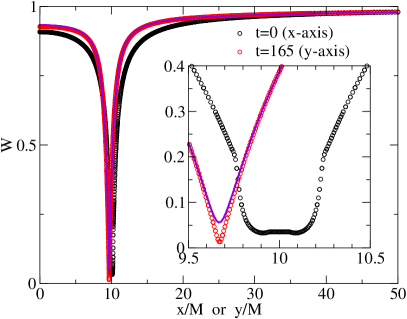
Figure 2: The metric function $W$ at $t=0$ plotted versus $x$ showing the effects of stuffing the BH interior and the same function at $t=165M$ (but plotted versus $y$). The more regular shape of $W$ near the center of the BH at $t=165M$ is typical of moving puncture simulations (note that the puncture is offset from the $y$ axis by $0.01M$). For reference, the function $W$ for a Bowen-York puncture simulation (solid curve) when the puncture crosses the $x$ axis for the second time is included (the plot of the Bowen-York data has been shifted). Note how the stuffed $W$ appears to evolve to be very similar to the standard trumpet $W$ typical of puncture initial data.

IV Simulations

The initial data parameters for our BHB simulations are given in Table 3. To evolve the second-order analytical data, we used the following grid structure: The coarsest grid spanned $0\leq x\leq 3200M$, $-3200M\leq y\leq 3200M$, and $0\leq z\leq 3200M$ (we used $\pi$-rotation symmetry and $z$-reflection symmetry). The refinement levels were centered on the two BHs with half-widths of 1600, 800, 440, 220, 110, 55, 25, 10, 5, 2, and 0.75. In the figures below we denote the resolution of the coarsest grid by $h$. Our lowest-resolution runs had a coarsest resolution of $h=h_{0}=32M$. We increased the resolution by successive factors of 1.2 for the higher-resolution runs. Our standard choice, which we used for all long-term runs shown below used a medium resolution of $h=h_{0}/1.2$. The highest-resolution run had $h=h_{0}/1.2^{3}$.

Table 3: Initial data parameters. $m_{1}$ and $m_{2}$ are the masses of the two BHs, $D$ is the orbital separation, $\delta\Omega_{\rm orb}$ and $\delta\dot{r}$ are the modifications to the 3.5PN orbital frequency and inspiral required to reduce the eccentricity, $\Xi$ is a scale factor (see text), and $r_{H}$ is the measured horizon radius.

$m_{1}/M$	$0.5$	$m_{2}/M$	$0.5$
$D/M$	$20.00$	$M\ \delta\Omega_{\rm orb}$	$7.88515\times 10^{-6}$
$\delta\dot{r}$	$-1.54103\times 10^{-4}$	$r_{\rm min}/M$	0.05
$r_{\rm max}/M$	0.25	$\Xi$	$800$
$r_{H}/M$	$0.484$

To demonstrate the smoothness of the transition from analytical to numerical evolution we, evolve a set of test particles using both the second-order analytic metric and the numerical evolution of the second-order analytic data. Note that at $t=0$, the 4-metrics associated with the two evolution schemes are geometrically identical (i.e., they only differ by a coordinate transformation implicit in using different choices for the lapse and shift at $t=0$). However, because the evolution schemes are different, the two spacetimes will have different effective stress energies (i.e., $G_{ab}$ will differ for the two spacetimes) even at $t=0$. Thus, even if the two spacetimes were initially in the same coordinate system, higher-order time derivatives (third and higher) of the geodesics will not agree. Thus, we only expect continuity of the force acting on the geodesics as we transition from analytical to numerical evolutions of the metric. As shown in Fig. 3, we do see a relatively smooth transition at early times with the two sets of geodesics initially agreeing quite well and then deviating more significantly at later times. Importantly, this latter deviation is due to two effects, differences in the later time coordinate systems and differences in the curvature. Plots of the same geodesics from the CCZ4 and BSSN evolutions are nearly identical.

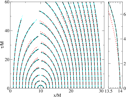
Figure 3: A set of timelike geodesics initially equally spaced in $x$ and normal to the $t=0$ hypersurface (note that one of the BHs is centered at $x=10M$ at $t=0$). Here the proper time of each geodesic is plotted as a function of the geodesic’s spatial position. The solid (black) curves correspond to geodesics evolved on the numerical spacetime using BSSN, the dot-dashed (cyan) curve correspond to the geodesics evolved on the numerical spacetime using CCZ4, finally the dotted (red) curves are for geodesics evolved with the second-order analytical metric. The plot to the right zooms in on a typical geodesic near the start of the simulation. Note how the numerical spacetime geodesics smoothly deviate from their analytical spacetime counterparts and there is no noticeable difference between the test particle trajectories for the BSSN and CCZ4 spacetimes at these early times. The rapid change in gauge near the start of the simulation is apparent in the smooth change in the geodesic seen at a proper time of about $\tau=3M$ in the inset.

Figure 3 provides evidence that the transition from analytical to numerical evolutions is sufficiently smooth that no sudden impulses are imparted to timelike geodesics. However, we still need to demonstrate that the subsequent dynamics are accurate. This will require that the constraint violations do not significantly affect the dynamics of the binary and that the binary remains quasicircular.

IV.1 Initial Hamiltonian and momentum constraint violations

Evolutions of second-order analytical data with BSSN were first performed in Tichy Reifenberger and Tichy (2012), where, like we do here, they looked at mass conservation, inspiral time, anomalous eccentricity, and constraint violations (see also Ref. Kelly et al. (2010)). The conclusion there, as well as here, is that residual constraint violations lead to relatively large errors in the subsequent dynamics.

Our expectation is that inaccuracies in the second-order analytic metric will decrease as the binary separation is increased. To test this assumption, we need a measure of the constraint violation that is related to the dynamics of the binary. Since we can interpret violations of the Hamiltonian constraint as an unphysical matter field on our spacetime, a natural measure of the degree of violation is the total amount of unphysical matter compared to the total amount of physical mass (in this case, the total amount of physical mass is $\approx 1M$). One subtlety we have to contend with is that both positive and negative mass densities are dynamically important, and there is no reason to expect their respective contributions to the total error will cancel. Thus, we consider two measures of the unphysical mass given by

$$m_{\rm unphys.} = \frac{1}{16\pi}\int{\cal H}\sqrt{\gamma}dv\,,$$ (5)

$$m_{\rm abs.} = \frac{1}{16\pi}\int|{\cal H}|\sqrt{\gamma}dv\,,$$ (6)

where ${\cal H}$ is the Hamiltonian constraint violation and the integral is over the cube centered on the origin with side length $400M$ excluding the interiors of the horizons. The former gives the net unphysical mass in the spacetime, while the absolute value in the latter ensures that positive and negative mass densities do not cancel.

We show both of these measures of unphysical mass versus separation in Fig. 4. Note that there is a near equal amount of positive and negative mass (which is why $m_{\rm unphys.}$ is about a factor of 20 smaller than $m_{\rm abs.}$). The magnitude of $m_{\rm unphys.}$ decreases with binary separation as roughly $(D/M)^{-1.8}$, while $m_{\rm abs.}$ decreases at the rate of $(D/M)^{-1.6}$. The masses were calculated at $t=0$ for three resolutions. In all cases, the truncation errors for the highest resolution corresponded to an uncertainty in the second or higher significant digit in the mass.

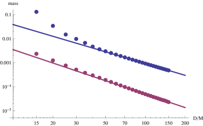
Figure 4: The unphysical mass of the binary versus binary separation $D$ for the second-order analytical data (i.e., initial data) as measured using the integrals $m_{\rm unphys.}$ and $m_{\rm abs.}$. The horizontal axis is in units of $D/M$, where $D$ is the separation of the binary. The larger mass is $m_{\rm abs.}$. Note that while a significant amount of unphysical matter is present, it is spread out such that only a fraction of it is absorbed by the BHs (see Fig. 5). Note also that there is a near equal amount of positive and negative mass (which is why $m_{\rm unphys.}$ is about a factor of 20 smaller than $m_{\rm abs.}$). Rather than plotting $m_{\rm unphys.}$, we plot $-m_{\rm unphys.}$, since the net unphysical mass is actually negative.

At a separation of $D=20M$, we find that $m_{\rm unphys.}=0.001M$, while $m_{\rm abs.}=0.033M$ (Bowen-York data for a $D=20M$ binary solved using the TwoPunctures Ansorg et al. (2004) code with $40^{3}$ collocation points gives $|m_{\rm abs.}|<7\times 10^{-7}M$). Note that $m_{\rm abs.}$ increases much more rapidly than the power-law prediction with decreasing separation for $D<25M$, but $m_{\rm unphys.}$ is only $30\%$ larger than the power-law prediction at $D=20M$. It is important to note that the BHs will not absorb this much mass, as their cross sections are quite small.

An important result from Fig. 4 is that while the unphysical mass tends to zero at infinite binary separation, for practical purposes, it is never small in the regime where we would use NR evolutions. Thus, we need a way of removing the unphysical mass from the system.

We also examine how the quantity of unphysical matter ($m_{\rm abs.}$) depends on the locations of the inner/near buffer zones. For our runs, we used the transition parameters of Ref. Johnson-McDaniel et al. (2009), which were optimized for a separation of $D=10M$. Using these parameters, we find that $m_{\rm abs.}$ is $0.033M$. By optimizing the parameters to reduce $m_{\rm abs.}$, we reduce this by only $4\%$ to $0.032M$. Interestingly, while $m_{\rm abs.}$ is reduced, the constraint violations are more concentrated near the two BHs, thus allowing for more absorption of constraint-violating matter by the BHs. Importantly, the constraint violations cannot be significantly reduced by moving the locations of the zone boundaries, since they are fixed analytic functions of the masses and separation delimiting overlapping regions of validity for different metric approximations.

It is important to determine not only how much unphysical matter is present, but also where it is located. To this end, we plot the Hamiltonian constraint violations on the equatorial plane for BHBs at separations of $D=20M$ and $D=100M$ using both the standard second-order analytical metric described in Sec. II and the first-order version. The main difference between the two is described in Table 2. The Hamiltonian constraint violations show a clear improvement as we switch from the first-order to the second-order analytical metric, indicating that it is the low PN order which dominates the error. Perhaps unexpectedly, even at a separation of $D=100M$, the first-order metric has $m_{\rm abs.}=0.02M$, while the second-order metric has $m_{\rm abs.}=0.001M$. Examining Fig. 5, we see that the constraint violations are concentrated in extended clouds well outside the horizons in the buffer zone between the inner and near zones. Most importantly, the first-order metric shows a strong shell of high constraint violation surrounding the two BHs. The second-order metric, on the other hand, has a lower-amplitude, more diffuse cloud of constraint violation that is less likely to be absorbed.

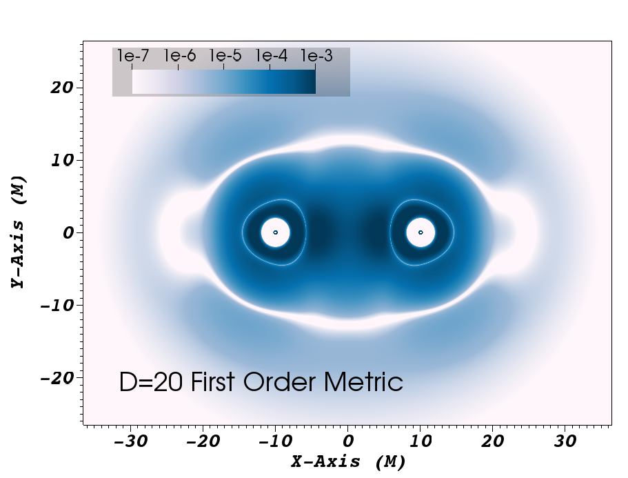
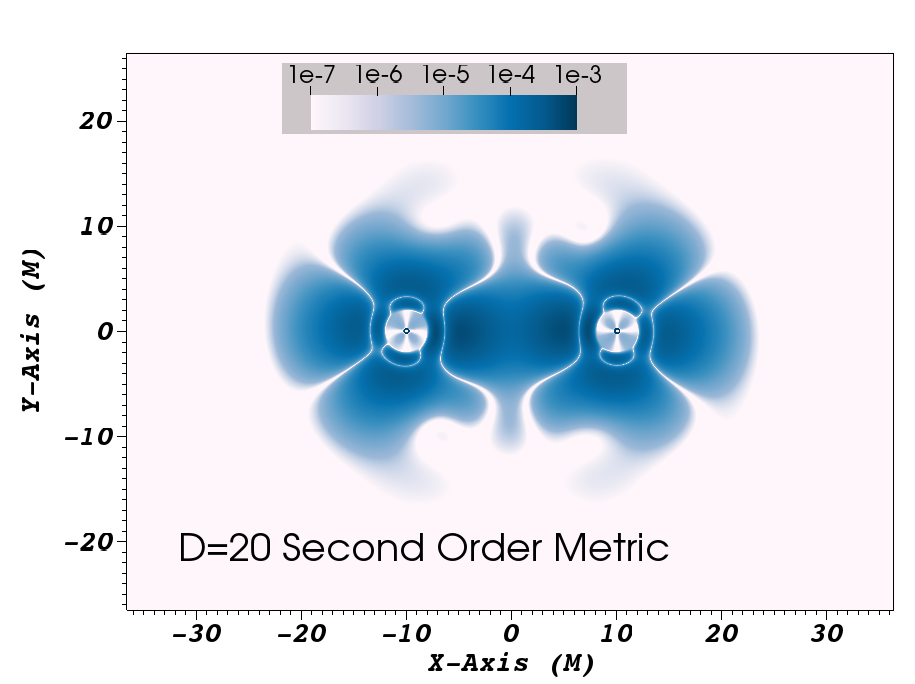
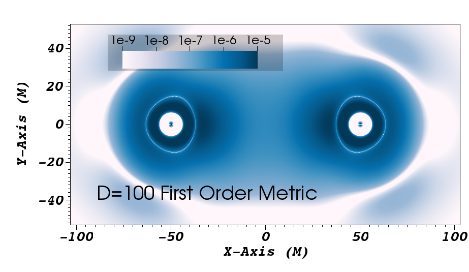
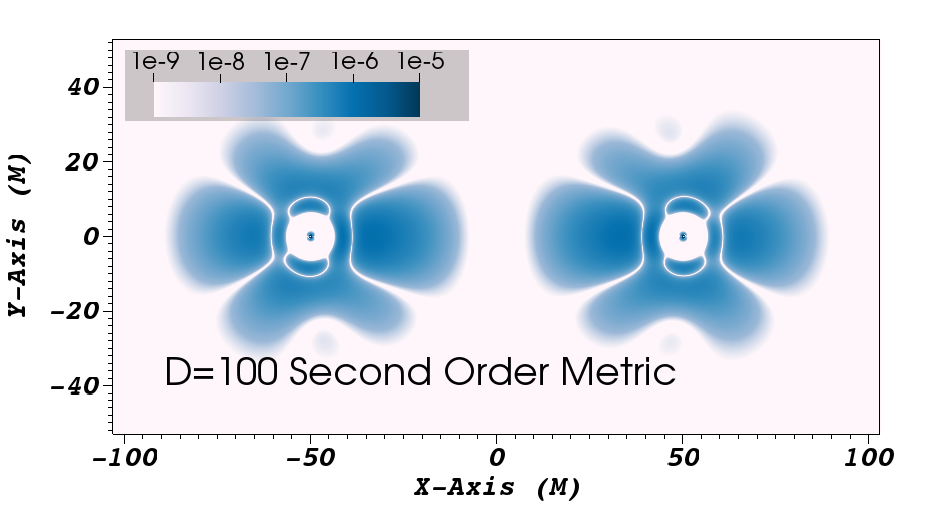
Figure 5: The Hamiltonian constraint violation in the vicinity of the two BHs in the binary for binary separations of $D=20M$ (top) and $D=100M$ (bottom). First-order metrics are shown to the left, and second-order metrics to the right. The very small white circles at the centers of the BHs are the horizons.

IV.2 Effects of the Hamiltonian and momentum constraint violations

In this section, we examine how the numerical evolution scheme can compound or mitigate issues associated with initial constraint violations. To this end, we evolved the second-order analytical data using both the BSSN formulation Nakamura et al. (1987); Shibata and Nakamura (1995); Baumgarte and Shapiro (1998) and the constraint-damping CCZ4 approach.

Our initial explorations of the dynamics of the second-order analytical data were based on the BSSN and CCZ4 systems. As shown in this section, we find that the CCZ4 is uniformly better than BSSN in evolving data with nontrivial constraint violations.

One of the most important differences between the BSSN and CCZ4 evolutions is in the horizon mass conservation. As shown in Fig. 6, the mass conservation of the BHs was relatively poor for BSSN and substantially better for CCZ4. In the figure, we see that the BSSN run showed an initial increase in mass of $10^{-3}M$, followed by a mass loss of similar magnitude. While a change of 2 parts in 1000 may seem small, the effect of this mass change on the orbital trajectory is quite large.

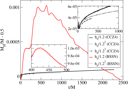
Figure 6: The individual apparent horizon masses for a BHB with initial separation of 20M for both CCZ4 (black) and BSSN (red) evolutions of the second-order analytical data. The BSSN curves show very large oscillations, while the CCZ4 curves show a much smaller linear growth. The large mass oscillations in the BSSN run are due to absorption of constraint violations. Note how the effects changing the evolution system from BSSN to CCZ4 are much larger than truncation error effects.

To determine the cause of the lack of conservation of the (apparent) horizon mass, we compare the time derivative of the horizon mass $dM_{H}/dt=dM_{1,2}/dt$ ($M_{1}=M_{2}$ by symmetry) with the average value of the constraint on the horizons ${\cal H}_{H}$ and the flux of constraint violation into the horizon ${\cal C}_{H}$ (since the spacetime around the two horizons is identical by symmetry, we only plot the constraint violation averaged over one of the BHs). We define ${\cal H}_{H}$ and ${\cal C}_{H}$ as

$${\cal H}_{H}=\frac{\oint{\cal H}\sqrt{\sigma}dAdB}{\oint\sqrt{\sigma}dAdB}\,,$$ (7)

$${\cal C}_{H}=-\oint{\cal C}^{i}n_{i}\sqrt{\sigma}dAdB\,,$$ (8)

where ${\cal H}$ is the Hamiltonian constraint violation, ${\cal C}^{i}$ is the momentum constraint violation, $n_{i}$ is the unit (outward) normal to the horizon, $\sqrt{\sigma}dAdB$ is the proper area element on the horizon, and the integrals are performed over the surface of the horizon.

In Fig. 7, we show the constraint violation averaged over the individual horizons for both BSSN and CCZ4. A large positive violation is observed at early times for BSSN, which is followed by a negative constraint violation. This links well with the initial increase in horizon mass for BSSN, which is followed by a later-time decrease. The CCZ4 constraints are a factor of 100 smaller and do not appear to be correlated with the CCZ4 horizon mass. Because of these results, all of our long-term simulations used CCZ4.

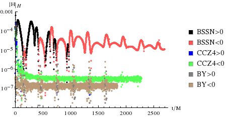
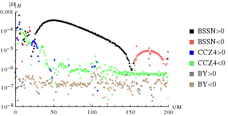
Figure 7: The Hamiltonian constraint averaged over the horizon as a function of time. This linear log plot shows the absolute value of the constraint violation for the BSSN and CCZ4 evolutions of the second-order analytic metric, as well as the evolution of Bowen-York data (BY) using CCZ4. The BSSN, CCZ4, and BY data points are colored according to the sign of the constraint violation. The lower plot shows the early-time behavior.

Aside from an overall positive (constant) numerical factor, plots of ${\cal H}_{H}$, ${\cal C}_{H}$, and $dM_{H}/dt$ are nearly identical for BSSN (see Fig. 8). This means that all three are strongly correlating (i.e., $dM_{H}/dt\propto{\cal C}_{H}\propto{\cal H}_{H}$). This provides a compelling argument that it is the constraint violations that cause the horizon masses to fluctuate. On the other hand, for CCZ4, there is no compelling correlation between $dM_{H}/dt$ and the (much smaller) constraint violations (see Fig. 9).

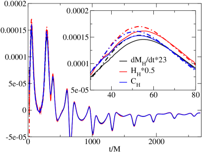
Figure 8: The Hamiltonian constraint averaged over the horizon, the flux of the momentum constraint violations through the horizon, and the time derivative of the horizon mass for the BSSN simulation. The Hamiltonian and change of rate of the horizon mass have been multiplied by constant positive factors. Note the near-perfect correlation of horizon mass change and constraint violation on the horizon. In the figure, solid curves correspond to a resolution of $h_{0}/1.2$, while dotted curves correspond to a resolution of $h_{0}/1.2^{2}$.

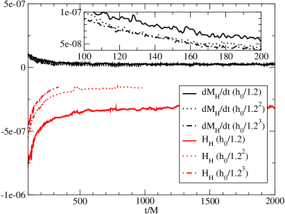
Figure 9: The Hamiltonian constraint averaged over the horizon and the time derivative of the horizon mass for the CCZ4 simulation. Note how unlike in Fig. 8, these two are not correlated. Here both the constraint violation and $\dot{m}$ appear to be converging to a very small value but from opposite directions.

Finally, we examine how the constraint violations in the bulk of the simulation domain behave with time. As shown in Fig. 10, the $L^{2}$ norms of the constraint violations for CCZ4 and BSSN evolutions behave quite differently (here we restrict the $L^{2}$ norm to the volume inside a ball of radius $30M$ and outside the two horizons so that the norm is dominated by constraint violations relatively close to the binary). The CCZ4 constraints fall to a much lower level (about a factor of 1000 smaller for the Hamiltonian and a factor of 100 for the momentum) than BSSN. For comparison purposes, we also performed equivalent evolutions with standard Bowen-York initial data Bowen and York (1980).

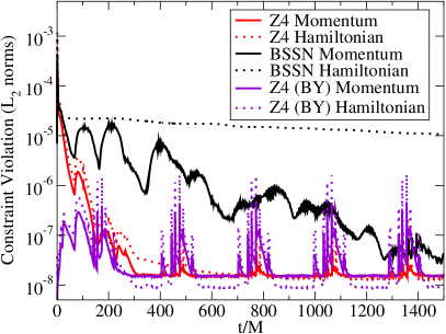
Figure 10: Time evolution of the $L^{2}$ norms of the constraint violations for BSSN and CCZ4 evolutions. Note how the BSSN Hamiltonian constraint remains relatively high while the CCZ4 constraints quickly fall to about $10^{-7}$. Also shown are the $L^{2}$ norms of the constraint violations for an evolution of Bowen-York data with CCZ4. The Bowen-York data leads to constraint violations that are on average a factor of 2 below constraint violations for the new data.

As shown in Fig. 11, we see clear convergence of the $L^{2}$ norm of the momentum constraint violation to zero for CCZ4, while the Hamiltonian constraint violation, though small, seems to bottom out at about $10^{-8}$. The Hamiltonian constraint for an equivalent Bowen-York run bottoms out at roughly half this value. For this convergence check, we only ran the highest-resolution run for 350M due to computational costs.

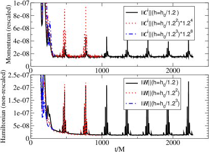
Figure 11: The $L^{2}$ norm of Hamiltonian constraint violations and the $L^{2}$ norm of the Euclidean magnitude of the momentum constraint violations. The momentum constraints have been rescaled by a factor of $(h_{0}/h)^{4}$, where $h$ is the base resolution of a particular run and $h_{0}$ is the base resolution of the coarsest simulation. Note that the Hamiltonian violations have not been rescaled. The spikes occurring roughly every 350M are due to the high-frequency initial gauge wave reflections off the mesh refinement boundaries. Here too, the $L^{2}$ norms have been restricted to the interior of a sphere of radius $30M$ about the origin and outside the two horizons

The amount of unphysical mass that the BHs can absorb depends not only on the amount of unphysical matter, but also on the dynamics of the unphysical matter. For BSSN, the constraint violations largely stay in place (and can therefore be accreted) due to the presence of a zero-speed constraint mode in BSSN Bernuzzi and Hilditch (2010), while for CCZ4 the constraints quickly leave the vicinity of the BHs. The very different behavior of BSSN and CCZ4 is shown in Fig. 12.

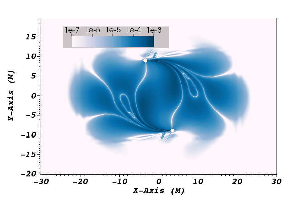
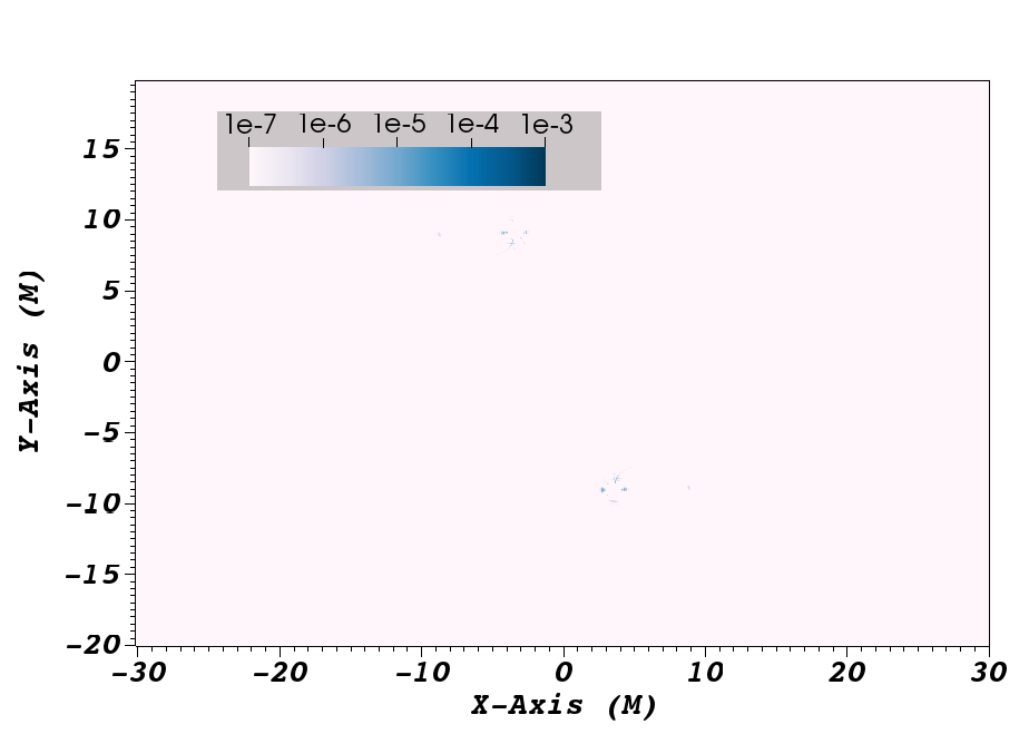
Figure 12: The Hamiltonian constraint on the $xy$ plane near the two BHs at $t=200M$ for the BSSN (left) and CCZ4 (right) evolutions of the second-order analytical data starting at a separation of $D=20M$. The scale is logarithmic and goes from $10^{-7}$ to $10^{-3}$. The absolute value of the constraint violations for the BSSN simulation match closely the violations on the initial slice, while the CCZ4 violations are three orders of magnitude smaller. In each plot the interiors of the BHs have been masked out. The constraint violations at $t=0$ are given in the top right plot in Fig. 5.

The overall efficacy of using CCZ4 to drive the constraint violations to zero can be measured by examining in detail how well the horizon masses are conserved. As shown in Figs. 13 and 14, there is a relatively strong linear trend in the mass that, while converging to a small value, is substantially larger than the Bowen-York result. Here we also see a significant advantage to using higher-order dissipation. Note that even with the highest-resolution runs, the horizon mass increase is an order of magnitude larger than for Bowen-York data evolved with CCZ4. Since the Bowen-York data were evolved with the same evolution system and grid structure, it appears that there are peculiarities associated with the analytic initial data driving the mass increase (note, as seen in Fig. 9, absorption of constraint violation seems not to be the cause of this mass increase). One possibility which we have not explored in detail here is that the methods used to stuff the BHs may be affecting the mass conservation. The other candidate would be residual constraint violations. Even for our highest-resolution run, the average constraint violation on the horizon surface at late times was 50% larger than for Bowen-York (the global constraint violations were, on average, an order of magnitude larger, as shown in Fig. 10). As observed in Ref. Zilhao et al. (2015), differences in accuracy of the spacetime at this level will likely not be important for MHD simulations.

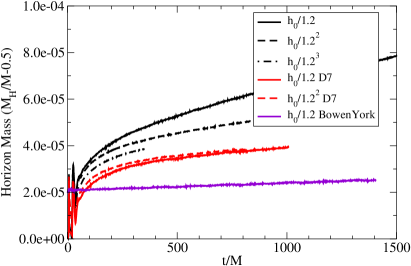
Figure 13: The mass of the individual horizons versus time for the CCZ4 simulations using the standard fifth-order dissipation, seventh-order dissipation, and fifth-order dissipation of Bowen-York data. The linear trend in the mass, while converging to a small value, is substantially larger than that for Bowen-York.

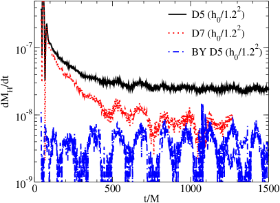
Figure 14: The rate of horizon mass increase versus time. Here D5 indicates that fifth-order dissipation was used, while D7 indicates that seventh-order was used.

IV.3 Eccentricity

As shown in Fig. 3, the transition from analytical to numerical evolutions is relatively smooth, and, as shown above, evolutions with CCZ4 drive the constraint violations down to acceptable levels (i.e., within a factor of 10 of the levels obtained by evolving the constraint satisfying Bowen-York data). The last step required for a successful continuation of the evolution is to ensure that the binary remains quasicircular (the PN inspiral used to generate the data is quasicircular). To accomplish this, we applied the eccentricity reduction procedure of Ref. Pfeiffer et al. (2007) to our data (we found that we needed to set $M\delta\Omega_{\rm orb}=7.88515\times 10^{-6}$ and $\delta\dot{r}=-1.54103\times 10^{-4}$). After three iterations, we were left with a residual eccentricity of $e=0.002$, which was small enough for this test (see, Fig. 15). In Fig. 15, we show the SPD versus time for both CCZ4 and BSSN evolutions of the eccentricity-reduced data, we also show a CCZ4 evolution of the original data. From the figure, the nonphysical dynamics (overall increase in radius) of the BSSN evolution is apparent. Note that we implement the eccentricity reduction by changing the initial orbital inspiral rate $\dot{r}$ and orbital frequency $\Omega_{\rm orb}$ used in the PN equations of motion. Changes to the inner-zone and far-zone metrics are automatically handled by the matching procedure.

The eccentricity reduction here is complicated by the fact that the amount of constraint-violating fields absorbed by the BHs changes as the trajectories are modified. This in turn, leads to a more complicated dependence of the eccentricity on the orbital parameters than is seen for constraint-satisfying data.

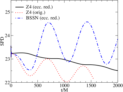
Figure 15: The SPD versus time as calculated using a CCZ4 evolution of the new data both before and after the eccentricity reduction procedure. For reference, a BSSN evolution of the low-eccentricity data is also given. Constraint violation drives the eccentricity for this latter case.

IV.4 Waveform

The waveforms presented below are relatively short (due to the expense of running the simulation to merger, which would take about six months on 80 Opteron cores). We will be comparing the numerical waveforms to PN waveforms. For these “short” runs, the dominant error is due to finite extraction radius. In Fig. 16, we show a “late” segment of the waveform extracted at $r=800M$, $r=1600M$, and a linear extrapolation (in $l=1/r$) to $r=\infty$ from these two waveforms, as well as the extrapolation to $r=\infty$ using the perturbative approach of Refs. Nakano et al. (2015); Nakano (2015). As expected, the dominant errors due to finite radius are phase errors. Finally, in Fig. 17, we show the waveform (post-initial burst) extracted at $r=800M$ for the resolutions $h=h_{0}/1.2^{2}$ and $h=h_{0}/1.2^{3}$. We also show the extrapolation of these waveforms using the techniques of Refs. Nakano et al. (2015); Nakano (2015). As can be seen, the dominant error in the waveform is the phase error due to finite extraction radius.

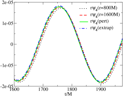
Figure 16: The $(\ell=2,\,m=2)$ mode of the waveform ($r\psi_{4}$) extracted at $r=800M$ and $r=1600M$, a linear extrapolation of these to $r=\infty$, and an extrapolation to $r=\infty$ using perturbative techniques. Both the standard extrapolation in $r$ and the perturbative approach give very similar waveforms.

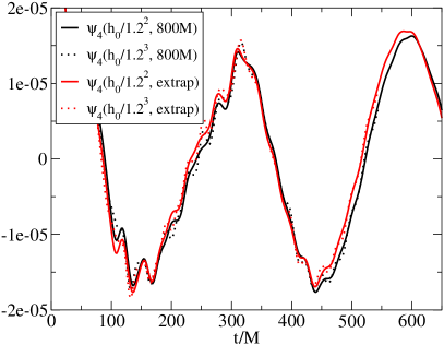
Figure 17: The $(\ell=2,\,m=2)$ mode of the waveform ($r\psi_{4}$) extracted at $r=800M$ at two resolutions. Both the raw waveform and the extrapolation to infinity are shown. The dominant error is the extrapolation error which manifests itself predominately as a phase error.

V Comparison to PN

To gauge the accuracy of our transition from analytical to numerical evolutions, we compare the subsequent dynamics of the binary with the predictions of PN.

In Fig. 18, we show the SPD versus time and PN separation versus time. Since the SPD at $t=0$ is larger than $20M$ we translate the SPD vertically. Note that the SPD is not expected to be equal to the PN separation. The SPD includes effects due to the nonflatness of the spatial metric and measures how distant the two horizons are from each other, while the PN separation extends from the center of one BH to the other and the proper separation corresponding to this would not be finite. While it is interesting that the numerical SPD matched the PN separation reasonably well, these are not gauge-invariant quantities. We also show the SPD for an equivalent Bowen-York simulation (evolved with BSSN) first reported in Ref. Lousto and Zlochower (2013). The Bowen-York run also had the eccentricity reduction procedure applied.

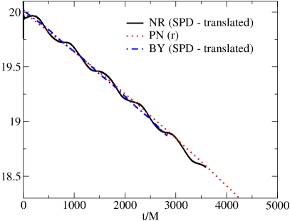
Figure 18: The SPD and PN separation versus time as calculated using a CCZ4 evolution of the new data and an older BSSN evolution of Bowen-York data. The SPD is always larger than the coordinate (and hence PN) separations. We shift the SPDs downward by $3.25M$ so that they agree with initial PN separation at $t=0$.

To have a more gauge-invariant measure of the accuracy of the evolution, we compare the waveform (as extracted at $1600M$) with the 3.5PN prediction for quasicircular orbits Faye et al. (2012) (similar to what was done in Refs. Lousto and Zlochower (2013) and Campanelli et al. (2009)). All waveforms are shown in Fig. 19.

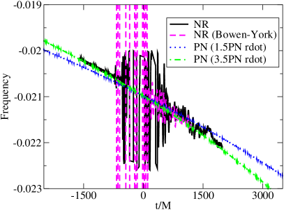
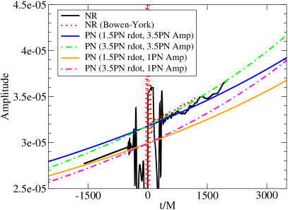
Figure 19: The frequency and magnitude of the $(\ell=2,m=2)$ mode of $r\psi_{4}$ as measured at $r=1600M$ in the full numerical simulation and various PN predictions. Here we use either the 1.5PN or 3.5PN expressions for $\dot{r}$ and either the full 3.5PN expression for $h_{22}$ (as a function of $r$ and $\omega$) of Faye et al. Faye et al. (2012), or we truncate to 1PN order. We use the 3PN expression for $\omega$ in all cases.

When extracting at $r=1600M$, we get very good agreement between the raw $(\ell=2,\,m=2)$ mode of $\psi_{4}$ and the extrapolation to infinity using the techniques of Ref. Nakano et al. (2015). Note that the numerical waveform prior to the burst of radiation is purely a function of the initial data. The initial data used the 3.5PN equations of motion; thus the agreement in the frequency at early times with 3.5PN is expected. On the other hand, the PM metric in the FZ contains terms up to 2.5PN order, which naturally leads to a lower-order approximation for the wave amplitude, since it depends not only on the orbital parameters, but also on the metric perturbation order. After the initial data burst, the waveform becomes noisier, but the agreement with 3.5PN is still quite good. The numerical waveform amplitude, however, seems to be closer to the average of 1.5PN and 3.5PN.

One important note is that the PN waveform given in the initial data is slightly out of phase with the resulting numerical waveform, as shown in Fig. 20. That is to say, after translating the waveform in time by $r^{*}$ (the tortoise coordinate of the extraction observer), the PN and NR waveforms agree quite well for the part of the waveform after the initial burst has hit the extraction sphere (in the plot, this would be from $t=0$ to $t=2400M$). However, prior to this burst arriving at the observer (in the plot, prior to $t=0$), the PN and NR waveforms are out of phase by $0.255$ radians. This initial part of the NR waveform is produced by the far-zone metric in the initial data, while the latter part of the waveform is produced by subsequent fully nonlinear binary dynamics. This will have repercussions if one wants to smoothly attach a PN waveform to the numerical waveform. It is important to note that other than a translation by the tortoise coordinate $r^{*}$ corresponding to the extraction radius, the NR and PN waveforms have not been translated.

The phase error itself can be explained by how we construct the metric in the far zone. In the far zone, the metric at some point at a (coordinate) distance $r$ from the origin depends on the dynamics of the binary at a retarded time given by the light propagation time from the binary to that point. We use the expression $t_{\rm ret}=t-r$, which is the flat-space retarded time. A more accurate expression would include the mass of the spacetime. For a Schwarzschild BH, in harmonic coordinates, the retarded time would be

$$t_{\rm ret}^{\rm Sch.}=t-\left[(r+M)+2M\log\left(\frac{r+M}{2M}-1\right)\right]\,,$$ (9)

where $M$ is the mass of the spacetime. We thus find that for a given waveform frequency $\omega$, using the flat-space retarded time will introduce a phase error of approximately

$$\delta\phi=\omega\left[M+2M\log\left(\frac{r+M}{2M}-1\right)\right]\,.$$ (10)

Since the binary’s orbital period here is $M\Omega_{\rm orb}\approx 0.01$, and the $(\ell=2,m=2)$ mode of the waveform has twice this frequency, we expect a phase error introduced by the flat space retarded time of $\approx 0.287$ radians, which is reasonably close to our measured phase error of $0.255$ radians.

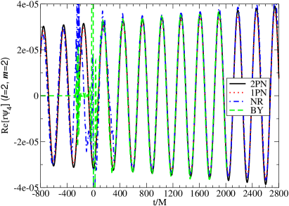
Figure 20: The numerical waveform from the new data, a numerical waveform from equivalent Bowen-York data, and the PN waveform. Here the numerical waveforms are shifted by $r^{*}$ (the tortoise coordinate at the extraction radius), and the PN waveform is unshifted. The phase agreement is good after $t=0$ but breaks down prior to the initial data pulse (for the new data) despite the fact that the NR frequency is in close agreement with PN for the whole waveform. The jump in phase between the early and late part of the waveform is likely due to the use of the flat-space retarded time in constructing the early waveform.

One final note concerns the amplitude of the initial data pulse in the waveform. As seen in Fig. 21, the initial pulse of radiation is suppressed relative to equivalent Bowen-York data. At $r=1600M$, the suppression is roughly a factor of $2$, while at the $r=400M$ extraction radius, the suppression is closer to a factor of 3. This is mostly due to the fact that we have initial data which model the astrophysical BHB system better and therefore possess less spurious radiation content when compared to the conformally flat BY initial data. Here, because of the resolution of the grid at $r=1600M$, the high-frequency gauge pulse (near $t=-500M$) is completely dissipated away. The high-frequency components of the initial data pulse are similarly suppressed.

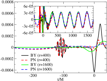
Figure 21: A plot of the real part of the $(\ell=2,m=2)$ mode of $r\psi_{4}$ (shifted in time by $-r$) for Bowen-York and the hybrid data here (denoted by PN). The waveforms extracted at $r=400M$ show a high-frequency pulse near $t=-100M$ due to an unresolved gauge wave. This high-frequency pulse is dissipated away and not visible in the waveform extracted at $r=1600M$.

VI Discussion

In order to perform accurate GRMHD simulations of gas accreting onto a BHB, including the minidisks around each BH, we need a spacetime that is accurate for the entire lifetime of the binary, i.e., from the slow inspiral at extremely large separation all the way to merger and relaxation of the remnant BH. Our goal, therefore, is to produce a four-dimensional metric that is accurate outside the horizons at all times, of sufficient smoothness that timelike geodesics vary smoothly (i.e., are $C^{\infty}$) except at a single transition time where they are $C^{2}$, and the subsequent binary dynamics should match PN predictions to a high degree in the vicinity of this transition time. To do this, we extended an analytic metric that is accurate when the binary’s separation is $D\gg M$ by continuing the evolution using fully nonlinear numerical techniques for closer separations.

The main questions we addressed here concerned how we can accurately transition from using an analytically evolved spacetime metric to a fully nonlinear numerically evolved metric that describes the binary during the rapid plunge and merger. At the transition, we used the analytical spacetime metric to construct initial data for a subsequent numerical evolution (as was previously done in Reifenberger and Tichy Reifenberger and Tichy (2012)). Our work builds upon Reifenberger and Tichy in two main ways. We start from an analytic spacetime that can be extended arbitrarily far into the past, and we can thus compare dynamics of particles pre- and post-transition. We also perform the transition at a binary separation of $D\sim 20M$, where the binary’s dynamics are still well described by PN theory and errors introduced in the gas dynamics by the approximate metric are washed out by MHD turbulence (see Ref. Zilhao et al. (2015) for an analysis of MHD evolutions on this analytical background for various separations).

In order for the transition from an analytical evolution to a numerical one to be smooth enough, the binary’s orbital dynamics could not change significantly as a result of the transition. The binary’s dynamics in the fully nonlinear numerical simulation had two main sources of error. First, constraint violations led to rapid unphysical oscillations in the orbital separation. Second, small errors in the PN expressions for the orbital angular momentum and inspiral rate led to eccentricity in the binary. We were able to ameliorate the first source of error by evolving with the constraint-damping CCZ4 Alic et al. (2012) formulation of the Einstein equations, which causes constraint violations to rapidly propagate away from the BHs, significantly reducing unphysical binary dynamics. In addition, by adding small changes to the initial inspiral rate and orbital frequency, we significantly reduced the eccentricity of the numerical binary using the techniques of Ref. Pfeiffer et al. (2007).

We subsequently found that the NR evolution leads to the expected gravitational waveform, orbital frequency, and binary inspiral rate (to within the truncation error of the simulation). The remaining error we found is a phase error in the early part of the waveform. This phase error is about $0.255$ radians. We ascribe this error to our use of the flat-space retarded time in the far-zone. By not including effects due to the mass of the spacetime we generate phase errors of the order of $0.287$ radians in the waveform. This error can itself be ameliorated by using the Schwarzschild retarded time when constructing the far-zone metric, which is something we will explore in an upcoming paper.