Bayesian model comparison with un-normalised likelihoods

Abstract

Models for which the likelihood function can be evaluated only up to a parameter-dependent unknown normalizing constant, such as Markov random field models, are used widely in computer science, statistical physics, spatial statistics, and network analysis. However, Bayesian analysis of these models using standard Monte Carlo methods is not possible due to the intractability of their likelihood functions. Several methods that permit exact, or close to exact, simulation from the posterior distribution have recently been developed. However, estimating the evidence and Bayes’ factors (BFs) for these models remains challenging in general. This paper describes new random weight importance sampling and sequential Monte Carlo methods for estimating BFs that use simulation to circumvent the evaluation of the intractable likelihood, and compares them to existing methods. In some cases we observe an advantage in the use of biased weight estimates. An initial investigation into the theoretical and empirical properties of this class of methods is presented. Some support for the use of biased estimates is presented, but we advocate caution in the use of such estimates.

1 Introduction

There has been much recent interest in performing Bayesian inference in models where the posterior is intractable and, in particular, we have the situation in which the posterior distribution $\pi(\theta|y)\propto p(\theta)f(y|\theta)$, cannot be evaluated pointwise. This intractability typically occurs occurs due to the intractability of the likelihood, i.e. $f(y|\theta)$ cannot be evaluated pointwise. Example scenarios include:

1. the use of big data sets, where $f(y|\theta)$ consists of a product of a large number of terms;

2. the existence of a large number of latent variables $x$, with $f(y|\theta)$ known only as a high dimensional integral $f(y|\theta)=\int_{x}f(y,x|\theta)dx$;

3. when $f(y|\theta)=\frac{1}{Z(\theta)}\gamma(y|\theta)$, with $Z(\theta)$ being an intractable normalising constant (INC) for the tractable term $\gamma(y|\theta)$ (e.g. when $f$ factorises as a Markov random field);

4. where it is possible to sample from $f(\cdot|\theta)$, but not to evaluate it, such as when the distribution of the data given $\theta$ is modelled by a complex stochastic computer model.

Each of these (overlapping) situations has been considered in some detail in previous work and each has inspired different methodologies.

In this paper we focus on the third case, in which the likelihood has an INC. This is an important problem in its own right (Girolami et al (2013) refer to it as “one of the main challenges to methodology for computational statistics currently”). There exist several competing methodologies for inference in this setting (see Everitt (2012)). In particular, the “exact” approaches of Møller et al (2006) and Murray et al (2006) exploit the decomposition $f(y|\theta)=\frac{1}{Z(\theta)}\gamma(y|\theta)$, whereas “simulation based” methods such as approximate Bayesian computation (ABC) (Grelaud et al, 2009) do not depend upon such a decomposition and can be applied more generally: to situation 1 in Picchini and Forman (2013); situations 2 and 3 (e.g. Everitt (2012)) and situation 4 (e.g. Wilkinson (2013)).

This paper considers the problem of Bayesian model comparison in the presence of an INC. We explore both exact and simulation-based methods, and find that elements of both approaches may also be more generally applicable. Specifically:

• For exact methods we find that approximations are required to allow practical implementation, and this leads us to investigate the use of approximate weights in importance sampling (IS) and sequential Monte Carlo (SMC). We examine the use of both exact-approximate approaches (as in Fearnhead et al (2010)) and also “inexact-approximate” methods, in which complete flexibility is allowed in the approximation of weights, at the cost of losing the exactness of the method. This work is a natural counterpart to Alquier et al (2015), which examines ananalogous question (concerning the acceptance probability) for Markov chain Monte Carlo (MCMC) algorithms. These generally applicable methods, “noisy MCMC” (Alquier et al, 2015) and “noisy SMC” (this paper) have some potential to address situations 1-3.

• We provide some comparison of these inexact approximations with simulation-based methods, including the “synthetic likelihood” (SL) of Wood (2010). In the applications considered here we find this to be a viable alternative to ABC. Our results are suggestive that this, and related methods, may find success in scenarios in which ABC is more usually applied.

In the remainder of this section we briefly outline the problem of, and methods for, parameter inference in the presence of an INC. We then detail the problem of Bayesian model comparison in this context, before discussing methods for addressing it in the following two sections.

1.1 Parameter inference

In this section we consider the problem of simulating from $\pi(\theta|y)\propto p(\theta)\gamma(y|\theta)/Z(\theta)$ using MCMC. This problem has been well studied, and such models are termed doubly intractable because the acceptance probability in the Metropolis-Hastings (MH) algorithm

$$\min\left\{1,\frac{q(\theta|\theta^{*})}{q(\theta^{*}|\theta)}\frac{p(\theta^{*})}{p(\theta)}\frac{\gamma(y|\theta^{*})}{\gamma(y|\theta)}\frac{Z(\theta)}{Z(\theta^{*})}\right\},$$ (1)

cannot be evaluated due to the presence of the INC. We first review exact methods for simulating from such a target in sections 1.1.1-1.1.3, before looking at simulation-based methods in sections 1.1.4 and 1.1.5. The methods described here in the context of MCMC form the basis of the methods for evidence estimation developed in the remainder of the paper.

1.1.1 Single and multiple auxiliary variable methods

Møller et al (2006) avoid the evaluation of the INC by augmenting the target distribution with an extra variable $u$ that lies on the same space as $y$, and use an MH algorithm with target distribution

$$\pi(\theta,u|y)\propto q_{u}(u|\theta,y)f(y|\theta)p(\theta),$$

where $q_{u}$ is some (normalised) arbitrary distribution. As the MH proposal in $(\theta,u)$-space they use

$$(\theta^{*},u^{*})\sim f(u^{*}|\theta^{*})q(\theta^{*}|\theta),$$

giving an acceptance probability of

$$\min\left\{1,\frac{q(\theta|\theta^{*})}{q(\theta^{*}|\theta)}\frac{p(\theta^{*})}{p(\theta)}\frac{\gamma(y|\theta^{*})}{\gamma(y|\theta)}\frac{q_{u}(u^{*}|\theta^{*},y)}{\gamma(u^{*}|\theta^{*})}\frac{\gamma(u|\theta)}{q_{u}(u|\theta,y)}\right\}.$$

Note that, by viewing $q_{u}(u^{*}|\theta^{*},y)/\gamma(u^{*}|\theta^{*})$ as an unbiased IS estimator of $1/Z(\theta^{*})$, this algorithm can be seen as an instance of the exact approximations described in Beaumont (2003) and Andrieu and Roberts (2009), where it is established that if an unbiased estimator of a target density is used appropriately in an MH algorithm, the $\theta$-marginal of the invariant distribution of this chain is the target distribution of interest. This automatically suggests extensions to the single auxiliary variable (SAV) method described above, where $M>1$ importance points are used, yielding:

$$\widehat{\frac{1}{Z(\theta)}}=\frac{1}{M}\sum_{m=1}^{M}\frac{q_{u}(u^{(m)}|\theta,y)}{\gamma(u^{(m)}|\theta)}.$$ (2)

Andrieu and Vihola (2012) show that the reduced variance of this estimator leads to a reduced asymptotic variance of estimators from the resultant Markov chain. The variance of the IS estimator is strongly dependent on an appropriate choice of IS target $q_{u}(\cdot|\theta,y)$, which should have lighter tails than $f(\cdot|\theta)$. Møller et al (2006) suggest that a reasonable choice may be $q_{u}(\cdot|\theta,y)=f(\cdot|\widehat{\theta})$, where $\widehat{\theta}$ is the maximum likelihood estimator of $\theta$. However, in practice $q_{u}(\cdot|\theta,y)$ can be difficult to choose well, particularly when $y$ lies on a high dimensional space. Motivated by this, annealed importance sampling (AIS) (Neal, 2001) can be used as an alternative to IS, leading to the multiple auxiliary variable (MAV) method of Murray et al (2006). AIS makes use of a sequence of $K$ targets, which in Murray et al (2006) are chosen to be

$$f_{k}(\cdot|\theta,\widehat{\theta},y) \propto \gamma_{k}(\cdot|\theta,\widehat{\theta},y)$$ (3)

$$= \gamma(\cdot|\theta){}^{(K+1-k)/(K+1)}q_{u}(\cdot|\theta,y){}^{k/(K+1)}$$

between $f(\cdot|\theta)$ and $q_{u}(\cdot|\theta,y)$. After the initial draw $u_{K+1}\sim f(\cdot|\theta)$, the auxiliary point is taken through a sequence of $K$ MCMC moves which successively have target $f_{k}(\cdot|\theta,\widehat{\theta},y)$ for $k=K:1$. The resultant IS estimator is given by

$$\widehat{\frac{1}{Z(\theta)}}=\frac{1}{M}\sum_{m=1}^{M}\prod_{k=1}^{K}\frac{\gamma_{k}(u_{k-1}^{(m)}|\theta,\widehat{\theta},y)}{\gamma_{k-1}(u_{k-1}^{(m)}|\theta,\widehat{\theta},y)}.$$ (4)

This estimator has a lower variance (although at a higher computational cost) than the corresponding IS estimator. We note that AIS can be viewed as a particular case of SMC without resampling and one might expect to obtain additional improvements at negligible cost by incorporating resampling steps within such algorithms (see Zhou et al (2015) for an illustration of the potential improvement and some discussion); we do not pursue this here as it is not the focus of this work.

1.1.2 Exchange algorithms

An alternative approach to avoiding the ratio of INCs in equation (1) is given by Murray et al (2006), in which it is suggested to use the acceptance probability

$$\min\left\{1,\frac{q(\theta|\theta^{*})}{q(\theta^{*}|\theta)}\frac{p(\theta^{*})}{p(\theta)}\frac{\gamma(y|\theta^{*})}{\gamma(y|\theta)}\frac{\gamma(u|\theta)}{\gamma(u|\theta^{*})}\right\},$$

where $u\sim f(\cdot|\theta^{*})$, motivated by the intuitive idea that $\gamma(u|\theta)/\gamma(u|\theta^{*})$ is a single point IS estimator of $Z(\theta)/Z(\theta^{*})$. This method is shown to have the correct invariant distribution, as is the extension in which AIS is used in place of IS. A potential extension might seem to be using multiple importance points $\{u^{(m)}\}_{m=1}^{M}\sim f(\cdot|\theta^{*})$ to obtain an estimator of $Z(\theta)/Z(\theta^{*})$ that has a smaller variance, with the aim of improving the statistical efficiency of estimators based on the resultant Markov chain. This scheme is shown to work well empirically in Alquier et al (2015). However, this chain does not have the desired target as its invariant distribution. Instead it can be seen as part of a wider class of algorithms that use a noisy estimate of the acceptance probability: noisy Monte Carlo algorithms (also referred to as “inexact approximations” in Girolami et al (2013)). Alquier et al (2015) shows that under uniform ergodicity of the ideal chain, a bound on the expected difference between the noisy and true acceptance probabilities can lead to bounds on the distance between the desired target distribution and the iterated noisy kernel. It also describes additional noisy MCMC algorithms for approximately simulating from the posterior, based on Langevin dynamics.

1.1.3 Russian Roulette and other approaches

Girolami et al (2013) use series-based approximations to intractable target distributions within the exact-approximation framework, where “Russian Roulette” methods from the physics literature are used to ensure the unbiasedness of truncations of infinite sums. These methods do not require exact simulation from $f(\cdot|\theta^{*})$, as do the SAV and exchange approaches described in the previous two sections. However, SAV and exchange are often implemented in practice by generating the auxiliary variables by taking the final point of a long “internal” MCMC run in place of exact simulation (e.g Caimo and Friel (2011)). For finite runs of the internal MCMC, this approach will not have exactly the desired invariant distribution, but Everitt (2012) shows that under regularity conditions the bias introduced by this approximation tends to zero as the run length of the internal MCMC increases: the same proof holds for the use of an MCMC chain for the simulation within an ABC-MCMC (i.e. MCMC applied to an ABC approximation of the posterior, Marjoram et al (2003)) or SL-MCMC (i.e. MCMC applied to an SL approximation) algorithm, as described in sections 1.1.4 and 1.1.5. Although the approach of Girolami et al (2013) is exact, as they note it is significantly more computationally expensive than this approximate approach. For this reason, we do not pursue Russian Roulette approaches further in this paper.

When a rejection sampler is available for simulating from $f(\cdot|\theta^{*})$, Rao et al (2013) introduce an alternative exact algorithm that has some favourable properties compared to the exchange algorithm. Since a rejection sampler is not available in many cases, we do not pursue this approach further.

1.1.4 Approximate Bayesian computation

Approximate Bayesian Computation (Tavaré et al, 1997) refers to methods that aim to approximate an intractable likelihood $f(y|\theta)$ through the integral

$$\widetilde{f}(S(y)|\theta)\propto\int\pi_{\epsilon}(S(y)|S(u))f(u|\theta)du$$ (5)

where $S(\cdot)$ gives a vector of summary statistics and $\pi_{\epsilon}\left(S(y)|S(u)\right)$ is the density of a symmetric kernel with bandwidth $\epsilon$, centered at $S(u)$ and evaluated at $S(y)$. As $\epsilon\rightarrow 0$, this distribution becomes more concentrated, so that in the case where $S(\cdot)$ gives sufficient statistics for estimating $\theta$, as $\epsilon\rightarrow 0$ the approximate posterior becomes closer to the true posterior. This approximation is used within standard Monte Carlo methods for simulating from the posterior. For example, it may be used within an MCMC algorithm, where using an exact-approximation argument it can be seen that it is sufficient in the calculation of the acceptance probability to use the Monte Carlo approximation

$$\widehat{f}_{\epsilon}(S(y)|\theta^{*})=\frac{1}{M}\sum_{m=1}^{M}\pi_{\epsilon}\left(S(y)\left|S\left(u^{(m)}\right)\right.\right)$$ (6)

for the likelihood at $\theta^{*}$ at each iteration, where $\{u^{(m)}\}_{m=1}^{M}\sim f(\cdot|\theta^{*})$. Whilst the exact-approximation argument means that there is no additional bias due to this Monte Carlo approximation, the approximation introduced through using a tolerance $\epsilon>0$ or insufficient summary statistics may be large. For this reason it might be considered a last resort to use ABC on likelihoods with an INC, but previous success on these models (e.g Grelaud et al (2009) and Everitt (2012)) lead us to consider them further in this paper.

1.1.5 Synthetic likelihood

ABC is essentially using, based on simulations from $f$, a nonparameteric estimator of $f_{S}\left(S|\theta\right)$, the distribution of the summary statistics of the data given $\theta$. In some situations, a parametric model might be more appropriate. For example, if the statistic is the sum of independent random variables, a Central Limit Theorem (CLT) might imply that it would be appropriate to assume that $f_{S}\left(S|\theta\right)$ is a multivariate Gaussian.

The SL approach (Wood, 2010) proceeds by making exactly this Gaussian assumption and uses this approximate likelihood within an MCMC algorithm. The parameters (the mean and variance) of this approximating distribution for a given $\theta$ are estimated based on the summary statistics of simulations $\{u^{(m)}\}_{m=1}^{M}\sim f(\cdot|\theta)$. Concretely, the estimate of the likelihood is

$$\widehat{f}_{\mbox{SL}}\left(S(y)|\theta\right)=\mathcal{N}\left(S(y);\widehat{\mu}_{\theta},\widehat{\Sigma}_{\theta}\right),$$

where

$$\widehat{\mu}_{\theta}= \frac{1}{M}\sum_{m=1}^{M}S\left(u^{(m)}\right) \widehat{\Sigma}_{\theta} =\frac{ss^{T}}{M-1},$$ (7)

with $s=\left(S\left(u_{1}\right)-\widehat{\mu}_{\theta},...,S\left(u_{M}\right)-\widehat{\mu}_{\theta}\right).$ Wood (2010) applies this method in a setting where the summary statistics are regression coefficients, motivated by their distribution being approximately normal. One of the approximations inherent in this method, as in ABC, is the use of summary statistics rather than the whole dataset. However, unlike ABC, there is no need to choose a bandwidth $\epsilon$: this approximation is replaced with that arising from the discrepancy between the normal approximation and the exact distribution of the chosen summary statistic. The SL method remains approximate even if the summary statistic distribution is Gaussian as $\widehat{f}_{\mbox{SL}}$ is not an unbiased estimate of the density and so the exact-approximation results do not apply. Rather, this is a special case of noisy MCMC, and we do not expect the additional bias introduced by estimating the parameters of $\widehat{f}_{\mbox{SL}}$ to have large effects on the results, even if the parameters are estimated via an internal MCMC chain targeting $f(\cdot|\theta)$ as described in section 1.1.3.

SL is related to a number of other simulation based algorithms under the umbrella of Bayesian indirect inference (Drovandi et al, 2015). This suggests a number of extensions to some of the methods presented in this paper that we do not explore here.

1.2 Bayesian model comparison

The main focus of this paper is estimating the marginal likelihood (also termed the evidence)

$$p(y)=\int p(\theta)f(y|\theta)d\theta$$

and Bayes’ factors: ratios of evidences for different models ($M_{1}$ and $M_{2}$, say), $\mbox{BF}_{12}={p(y|M_{1})}/{p(y|M_{2})}$. These quantities cannot usually be estimated reliably from MCMC output, and commonly used methods for estimating them require $f(y|\theta)$ to be tractable in $\theta$. This leads Friel (2013) to label their estimation as “triply intractable” when $f$ has an INC. To our knowledge the only published approach to estimating the evidence for such models is in Friel (2013), with this paper also giving one of the only approaches to estimating BFs in this setting. For estimating BFs, ABC provides a viable alternative (Grelaud et al, 2009), at least for models within the exponential family.

Friel (2013) starts from Chib’s approximation,

$$\widehat{p}(y)=\frac{f(y|\widetilde{\theta})p(\widetilde{\theta})}{\widehat{\pi}(\widetilde{\theta}|y)},$$ (8)

where $\widetilde{\theta}$ can be an arbitrary value of $\theta$ and $\widehat{\pi}$ is an approximation to the posterior distribution. Such an approximation is intractable when $f$ has an INC. Friel (2013) devises a “population” version of the exchange algorithm that simulates points $\theta^{(p)}$ from the posterior distribution, and which also gives an estimate $\widehat{Z}(\theta^{(p)})$ of the INC at each of these points. The points $\theta^{(p)}$ can be used to find a kernel density approximation $\widehat{\pi}$, and estimates $\widehat{Z}(\theta^{(p)})$ of the INC. These are then used in a number of evaluations of (8) at points (generated by the population exchange algorithm) in a region of high posterior density, which are then averaged to find an estimate of the evidence. This method has a number of useful properties (including that it may be a more efficient approach for parameter inference than the standard exchange algorithm), but for evidence estimation it suffers the limitation of using a kernel density estimate which means that, as noted in the paper, its use is limited to low-dimensional parameter spaces.

In this paper we explore the alternative approach of methods based on IS, making use of the likelihood approximations described earlier in this section. These IS methods are outlined in section 2. In section 2 we note the good empirical performance of an inexact-approximate method and examine such approaches in more detail. As IS is itself not readily applicable to high dimensional parameter spaces, in section 3 we look at natural extensions to the IS methods based on SMC. Particular care is required when considering approximations within iterative algorithms: we provide a preliminary study of approximation in this context demonstrating theoretically that the resulting error can be controlled uniformly in time, under very favorable assumptions. This, and the associated empirical study are intended to provide motivation and proof of concept; caution is still required if approximation is used within such methods in practice but the results presented suggest that further investigation is warranted. The algorithms presented later in the paper are viable alternatives to the MCMC approaches to parameter estimation described in this section, and may outperform the corresponding MCMC approach in some cases. In particular they all automatically make use of a population of points, an idea previously explored in the MCMC context by Caimo and Friel (2011) and Friel (2013). In section 4 we draw conclusions.

2 Importance sampling approaches

In this section we investigate the use of IS for estimating the evidence and BFs for models with INCs. We consider an “ideal” importance sampler that simulates $P$ points $\left\{\theta^{(p)}\right\}_{p=1}^{P}$ from a proposal $q(\cdot)$ and calculates their weight, in the presence of an INC, using

$$\widetilde{w}^{(p)} = \frac{p(\theta^{(p)})\gamma(y|\theta^{(p)})}{q(\theta^{(p)})Z(\theta^{(p)})},$$ (9)

with an estimate of the evidence given by

$$\widehat{p}(y)=\frac{1}{P}\sum_{p=1}^{P}\widetilde{w}^{(p)}.$$ (10)

To estimate a BF we simply take the ratio of estimates of the evidence for the two models under consideration. However, the presence of the INC in the weight expression in (9) means that importance samplers cannot be directly implemented for these models. To circumvent this problem we will investigate the use of the techniques described in section 1.1 in importance sampling. We begin by looking at exact-approximation based methods in section 2.1. We then examine the use to approximate likelihoods based on simulation, including ABC and SL in section 2.2, before looking at the performance of all of these methods on a toy example in section 2.3. Finally, in sections 2.4 and 2.6 we examine applications to exponential random graph models (ERGMs) and Ising models, the latter of which leads us to consider the use of inexact-approximations in IS (first introduced in section 2.5).

2.1 Auxiliary variable IS

To avoid the evaluation of the INC in (9), we propose the use of the auxiliary variable method used in the MCMC context in section 1.1.1. Specifically, consider IS using the SAV target

$$p(\theta,u|y)\propto q_{u}(u|\theta,y)f(y|\theta)p(\theta),$$

noting that it has the same normalizing constant as $p(\theta|y)\propto f(y|\theta)p(\theta)$, with proposal

$$q(\theta,u)=f(u|\theta)q(\theta).$$

This results in weights

$$\widetilde{w}^{(p)} = \frac{q_{u}(u|\theta^{(p)},y)\gamma(y|\theta^{(p)})p(\theta^{(p)})}{\gamma(u|\theta^{(p)})q(\theta^{(p)})}\frac{Z(\theta^{(p)})}{Z(\theta^{(p)})}$$

$$= \frac{\gamma(y|\theta^{(p)})p(\theta^{(p)})}{q(\theta^{(p)})}\frac{q_{u}(u|\theta^{(p)},y)}{\gamma(u|\theta^{(p)})},$$

and the estimate (10) of the evidence.

In this method, which we will refer to as single auxiliary variable IS (SAVIS), we may view $q_{u}(u|\theta^{(p)},y)/\gamma(u|\theta^{(p)})$ as an unbiased importance sampling (IS) estimator of $1/Z(\theta^{(p)})$. Although we are using an unbiased estimator of the weights in place of the ideal weights, the result is still an exact importance sampler. SAVIS is an exact-approximate IS method, as seen previously in Fearnhead et al (2010), Chopin et al (2013) and Tran et al (2013). As in the MCMC setting, to ensure the variance of estimators produced by this scheme is not large we must ensure the variance of estimator of $1/Z(\theta^{(p)})$ is small. Thus in practice we found extensions to this basic algorithm were useful: using multiple $u$ importance points for each proposed $\theta^{(p)}$ as in (2); and using AIS, rather than simple IS, for estimating $1/Z(\theta^{(p)})$ as in (4) (giving an algorithm that we refer to as multiple auxiliary variable IS (MAVIS), in common with the terminology in Murray et al (2006)). Using $q_{u}(\cdot|\theta,y)=f(\cdot|\widehat{\theta})$, as described in section 1.1.1, and $\gamma_{k}$ as in (3), we obtain

$$\widehat{\frac{1}{Z(\theta)}}=\frac{1}{Z(\widehat{\theta})}\frac{1}{M}\sum_{m=1}^{M}\prod_{k=1}^{K}\frac{\gamma_{k}(u_{k-1}^{(m)}|\theta^{*},\theta,y)}{\gamma_{k-1}(u_{k-1}^{(m)}|\theta^{*},\theta,y)}.$$ (11)

In this case the (A)IS methods are being used as unbiased estimators of the ratio $Z(\widehat{\theta})/Z(\theta)$ and again SMC could be used in their place.

2.2 Simulation based methods

Didelot et al (2011) investigate the use of the ABC approximation when using IS for estimating marginal likelihoods. In this case the weight equation becomes

$$\widetilde{w}^{(p)}=\frac{p(\theta^{(p)})\frac{1}{R}\sum_{r=1}^{R}\pi_{\epsilon}(S(y)|S(x_{r}^{(p)}))}{q(\theta^{(p)})},$$

where $\left\{x_{r}^{(p)}\right\}_{r=1}^{R}\sim f(\cdot|\theta^{(p)})$, and using the notation from section 1.1.4. However, using these weights within (10) gives an estimate for $p(S(y))$ rather than, as desired, an estimate of the evidence $p(y)$.

Fortunately, there are cases in which ABC may be used to estimate BFs. Didelot et al (2011) establish that, for the BF for two exponential family models: if $S_{1}(y)$ is sufficient for the parameters in model 1 and $S_{2}(y)$ is sufficient for the parameters in model 2, then using $S(y)=(S_{1}(y),S_{2}(y))$ gives

$$\frac{p(y|M_{1})}{p(y|M_{2})}=\frac{p(S(y)|M_{1})}{p(S(y)|M_{2})}.$$

Outside the exponential family, making an appropriate choice of summary statistics is harder (Robert et al, 2011; Prangle et al, 2014; Marin et al, 2014).

Just as in the parameter estimation case, the use of a tolerance $\epsilon>0$ results in estimating an approximation to the true BF. An alternative approximation, not previously used in model comparison, is to use SL (as described in section 1.1.5). In this case the weight equation becomes

$$\widetilde{w}^{(p)}=\frac{p(\theta^{(p)})\mathcal{N}\left(S(y);\widehat{\mu}_{\theta^{(p)}},\widehat{\Sigma}_{\theta^{(p)}}\right)}{q(\theta^{(p)})},$$

where $\widehat{\mu}_{\theta},\widehat{\Sigma}_{\theta}$ are given by (7). As in parameter estimation, this approximation is only appropriate if the normality assumption is reasonable. The choice of summary statistics is as difficult as in the ABC case.

2.3 Toy example

In this section we have discussed three alternative methods for estimating BFs: MAVIS, ABC and SL. To further understand their properties we now investigate the performance of each method on a toy example.

Consider i.i.d. observations $y=\left\{y_{i}\right\}_{i=1}^{n=100}$ of a discrete random variable that takes values in $\mathbb{N}$. For such a dataset, we will find the BF for the models

1. $y|\theta\sim\mbox{Poisson}(\theta)$, $\theta=\lambda\sim\mbox{Exp}(1)$

   $$f_{1}\left(y|\theta\right) = \prod_{i=1}^{n}\frac{\lambda^{y_{i}}}{y_{i}!}/\exp(-n\lambda)$$

2. $y|\theta\sim\mbox{Geometric}(\theta)$, $\theta=p\sim\mbox{Unif}(0,1)$

   $$f_{2}\left(y|\theta\right) = \prod_{i=1}^{n}(1-p)^{y_{i}}/p^{-n}.$$

In both cases we have rewritten the likelihoods $f_{1}$ and $f_{2}$ in the form $\gamma(y|\theta)/Z(\theta)$ in order to use MAVIS. Due to the use of conjugate priors the BF for these two models can be found analytically. As in Didelot et al (2011) we simulated (using an approximate rejection sampling scheme) 1000 datasets for which $\frac{p(y|M_{1})}{p(y|M_{1})+p(y|M_{2})}$ roughly uniformly cover the interval [0.01,0.99], to ensure that testing is performed in a wide range of scenarios. For each algorithm we used the same computational effort, in terms of the number of simulations ($100,000$) from the likelihood (such simulations dominate the computational cost of all of the algorithms considered).

Our results are shown in figure 1, with the algorithm-specific parameters being given in figure 1a. We note that we achieved better results for MAVIS when: devoting more computational effort to the estimation of $1/Z(\theta)$ (thus we used only 100 importance points in $\theta$-space, compared to 1000 for the other algorithms); and using more intermediate bridging distributions in the AIS, rather than multiple importance points (thus, in equation (11) we used $K=1000$ and $M=1$). In the ABC case we found that reducing $\epsilon$ much further than 0.1 resulted in many importance points with zero weight (note that here, and throughout the paper we use the uniform kernel for $\pi_{\epsilon}$). From the box plots in figure 1a, we might infer that overall SL has outperformed the other methods, but be concerned about the number of outliers. Figures 1b to 1d shed more light on the situations in which each algorithm performs well.

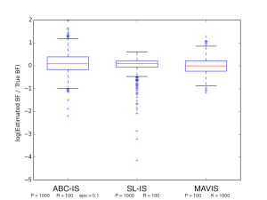
(a) A box plot of the $\log$ of the estimated BF divided by the true BF.

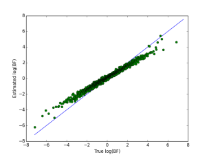
(b) The $\log$ of the BF estimated by ABC-IS against the $\log$ of the true BF.

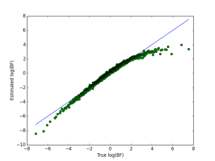
(c) The $\log$ of the BF estimated by SL-IS against the $\log$ of the true BF.

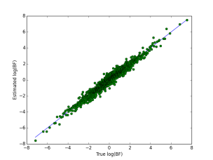
(d) The $\log$ of the BF estimated by MAVIS against the $\log$ of the true BF.

Figure 1: Bayes’ factors for the Poisson and geometric models.

In figure 1b we observe that the non-zero $\epsilon$ results in a bias in the BF estimates (represented by the shallower slope in the estimated BFs compared to the true values). In this example we conclude that ABC has worked quite well, since the bias is only pronounced in situations where the true BF favours one model strongly over the other, and this conclusion would not be affected by the bias. For this reason it might be more relevant in this example to consider the deviations from the shallow slope, which are likely due to the Monte Carlo variance in the estimator (which becomes more pronounced as $\epsilon$ is reduced). We see that the choice of $\epsilon$ essentially governs a bias-variance trade-off, and that the difficulty in using the approach more generally is that it is not easy to evaluate whether a choice of $\epsilon$ that ensures a low variance also ensures that the bias is not significant in terms of affecting the conclusions that might be drawn from the estimated BF (see section 2.4). Figure 1c suggests that SL has worked extremely well (in terms of having a low variance) for the most important situations, where the BF is close to 1. However, we note that the large biases introduced due to the limitation of the Gaussian assumption when the BF is far from 1. Figure 1d indicates that there is little or no bias when using MAVIS, but that there is appreciable variance (due to using IS on the relatively high-dimensional $u$-space).

These results highlight that the three methods will be most effective in slightly different situations. The approximations in ABC and SL introduce a bias, the effect of which might be difficult to assess. In ABC (assuming sufficient statistics) this bias can be reduced by an increased computational effort allowing a smaller $\epsilon$, however it is essentially impossible to assess when this bias is “small enough”. SL is the simplest method to implement, and seems to work well in a wide variety of situations, but the advice in Wood (2010) should be followed in checking that the assumption of normality is appropriate. MAVIS is limited by the need to perform importance sampling on the high-dimensional $(\theta,u)$ space but consequently avoids specifying summary statistics, its bias is small, and this method is able to estimate the evidence of individual models.

2.4 Application to social networks

In this section we use our methods to compare the evidence for two alternative ERGMs for the Gamaneg data previously analysed in Friel (2013) (who illustrate the data in their figure 3). An ERGM has the general form

$$f(y|\theta)=\frac{1}{Z(\theta)}\exp\left(\theta^{T}S(y)\right),$$

where $S(y)$ is a vector of statistics of a network $y$ and $\theta$ is a parameter vector of the same length. We take $S(y)=$ $(\#$ of edges $)$ in model 1 and $S(y)=($# of edges, # of two stars$)$ in model 2 . As in Friel (2013) we use the prior $p(\theta)=\mathcal{N}(\theta;0,25I)$.

Using a computational budget of $10^{5}$ simulations from the likelihood (each simulation consisting of an internal MCMC run of length 1000 as a proxy for an exact sampler, as described in section 1.1.3), Friel (2013) finds that the evidence for model 1 is $\sim 37\times$ that for model 2. Using the same computational budget for our methods, consisting of 1000 importance points (with 100 simulations from the likelihood for each point), we obtained the results shown in Table 1.

	ABC ($\epsilon=0.1$)	ABC ($\epsilon=0.05$)	SL	MAVIS
$\frac{\hat{p}(y|M_{1})}{\hat{p}(y|M_{2})}$	4	20	40	41

Table 1: Model comparison results for Gamaneg data. Note that the ABC ($\epsilon=0.05$) estimate was based upon just 5 sample points of non-zero weight. MAVIS also provides estimates of the individual evidence ($\log\left[\widehat{p}(y|M_{1})\right]=-69.6$, $\log\left[\widehat{p}(y|M_{2})\right]=-73.3$).

This example highlights the issue with the bias-variance trade-off in ABC, with $\epsilon=0.1$ having too large a bias and $\epsilon=0.05$ having too large a variance. SL performs well — in this particular case the Gaussian assumption appears to be appropriate. One might expect this, since the statistics are sums of random variables. However, we note that this is not usually the case for ERGMs, particularly when modelling large networks, and that SL is a much more appropriate method for inference in the ERGMs with local dependence (Schweinberger and Handcock, 2015). A more sophisticated ABC approach might exhibit improved performance, possibly outperforming SL. However, the appeal of SL is in its simplicity, and we find it to be a useful method for obtaining good results with minimal tuning.

2.5 IS with biased weights

The implementation of MAVIS in the previous section is not an exact-approximate method for two reasons:

1. An internal MCMC chain was used in place of an exact sampler;

2. The $1/Z(\widehat{\theta})$ term in (11) was estimated before running this algorithm (by using a standard SMC method, with initial distribution being the Bernoulli random graph (which can be simulated from exactly) and final distribution $\propto\gamma(\cdot|\widehat{\theta})$ to estimate $Z(\widehat{\theta})$ (being the normalising constant of $\gamma$), and taking the reciprocal) with this fixed estimate being used throughout.

However, in practice, we tend to find that such “inexact-approximations” do not introduce large errors into Bayes’ factor estimates, particularly when compared to standard implementations of ABC (as seen in the previous section).

This example suggests that in practice it may sometimes be advantageous to use biased rather than unbiased estimates of importance weights within a random weight IS algorithm: an observation that is somewhat analogous to that made in Alquier et al (2015) in the context of MCMC. This section provides an initial theoretical exploration as to whether this might be a useful strategy in IS.

In order to analyse the behaviour of importance sampling with biased weights, we consider biased estimates of the weights in equation (10). Let

$$w(\theta):=\frac{p(\theta)\gamma(y|\theta)}{Z(\theta)q(\theta)}.$$

We consider biased randomised weights that admit an additive decomposition,

$$\grave{w}(\theta):=w(\theta)+b(\theta)+\grave{V}_{\theta},$$

in which $b(\theta)=\mathbb{E}[\grave{w}(\theta)|\theta]-w(\theta)$ is a deterministic function describing the bias of the weights and $\grave{V}_{\theta}$ is a random variable (more precisely, there is an independent copy of such a random variable associated with every particle), which conditional upon $\theta$ is of mean zero and variance $\grave{\sigma}_{\theta}^{2}=\textrm{Var}(\grave{w}(\theta)|\theta)$. This decomposition will not generally be available in practice, but is flexible enough to allow the formal description of many settings of interest. For instance, one might consider the algorithms presented here by setting $b(\theta)$ to the (conditional) expected value of the difference between the approximate and exact weights and $\grave{V}_{\theta}$ to the difference between the approximate weights and their expected value.

We have immediately that the bias of such an estimate is, using a subscript of $q$ to denote expectations and variances with respect to $q(\theta)$, $\mathbb{E}_{q}[b(\theta)]$. By a simple application of the law of total variance, its variance is

$$\frac{1}{P}\textrm{Var}_{q}(\grave{w}(\theta))=\frac{1}{P}\left\{\textrm{Var}_{q}\left[w(\theta)+b(\theta)\right]+\mathbb{E}_{q}\left[\grave{\sigma}_{\theta}^{2}\right]\right\}$$

Consequently, the mean squared error of this estimate is:

$$\frac{1}{P}\left\{\textrm{Var}_{q}\left[w(\theta)+b(\theta)\right]+\mathbb{E}_{q}[\grave{\sigma}_{\theta}^{2}]\right\}+\mathbb{E}_{q}[b(\theta)]^{2}.$$

If we compare such a biased estimator with a second estimator in which we use the same proposal distribution but instead use an unbiased random weight

$$\acute{w}(\theta):=w(\theta)+\acute{V}(\theta),$$

where $\acute{V}(\theta)$ has conditional expectation zero and variance $\acute{\sigma}_{\theta}^{2}$, then it’s clear that the biased estimator has smaller mean squared error for small enough samples if it has sufficiently smaller variance, i.e., when (assuming $\mathbb{E}_{q}[b(\theta)]^{2}>0$, otherwise one estimator dominates the other for all sample sizes):

$$\frac{1}{P}\left\{\textrm{Var}_{q}\left[w(\theta)+b(\theta)\right]+\mathbb{E}_{q}[\grave{\sigma}_{\theta}^{2}]\right\}+\mathbb{E}_{q}[b(\theta)]^{2}$$

$$< \frac{1}{P}\left\{\textrm{Var}_{q}\left[w(\theta)\right]+\mathbb{E}_{q}[\acute{\sigma}_{\theta}^{2}]\right\}$$

which holds when $P$ is inferior to

$$\frac{\mathbb{E}_{q}[\acute{\sigma}_{\theta}^{2}-\grave{\sigma}_{\theta}^{2}]-\textrm{Var}_{q}\left[b(\theta)\right]-2\textrm{Cov}_{q}\left[w(\theta),b(\theta)\right]}{\mathbb{E}_{q}[b(\theta)]^{2}}.$$

In the artificially simple setting in which $b(\theta)=b_{0}$ is constant, this would mean that the biased estimator would have smaller MSE for samples smaller than the ratio of the difference in variance to the square of that bias suggesting that qualitatively a biased estimator might be better if the square of the average bias is small in comparison to the variance reduction that it provides. Given a family of increasingly expensive biased estimators with progressively smaller bias, one could envisage using such an argument to manage the trade-off between less biased estimators and larger sample sizes. In practice a negative covariance between $b(\theta)$ and $w(\theta)$ might also lead to favourable performance by biased estimators.

2.6 Applications to Ising models

In the current section we investigate this type of approach further empirically, estimating Bayes’ factors from data simulated from Ising models. In particular we reanalyse the data from Friel (2013), which consists of 20 realisations from a first-order $10\times 10$ Ising model and 20 realisations from a second-order $10\times 10$ Ising model for which accurate estimates (via Friel and Rue (2007)) of the evidence serve as a ground truth for comparison. We also analyse data from a $100\times 100$ Ising model.

2.6.1 $10\times 10$ Ising models

As in the toy example, we examine several different configurations of the IS and AIS estimators of the $Z(\widehat{\theta})/Z(\theta)$ term in the weight (9), using different values of $M$, $K$ and $B$, the burn in of the internal MCMC, that yield the same computational cost (in terms of the number of Gibbs sweeps used to simulate from the likelihood). Note that for small values of $B$ these estimators are biased; a bias that decreases as $B$ increases.

The empirical results in Friel (2013), use a total $2\times 10^{7}$ Gibbs sweeps to estimate one Bayes’ factor, to allow comparison of our results with those in that paper. Here, estimating a marginal likelihood is done in three stages: firstly $\widehat{\theta}$ is estimated; followed by $Z(\widehat{\theta})$, then finally the marginal likelihood. We took $\widehat{\theta}$ to be the posterior expectation, estimated from a run of the exchange algorithm of $10,000$ iterations. $Z(\widehat{\theta})$ was then estimated using SMC with an MCMC move, with 200 particles and 100 targets, with the $i$th target being $\gamma_{i}(\cdot|\theta)=\gamma_{i}\left(\cdot|{i\theta}/{100}\right)$, employing stratified resampling when the effective sample size (ESS; Kong et al (1994)) falls below 100. The total cost of these three stages is $5\times 10^{6}$ Gibbs sweeps ($1/4$ of the cost of population exchange) with the final IS stage costing $2\times 10^{4}$ sweeps ($1/1000$ of the cost of population exchange). We note that the cost of the first two stages has been chosen conservatively - less computational effort here can also yield good results. The importance proposal used in all cases was a multivariate normal distribution, with mean and variance taken to be the sample mean and variance from the initial run of the exchange algorithm. This proposal would clearly not be appropriate in high dimensions, but is reasonable for the low dimensional parameter spaces considered here. Figure 2 shows the results produced by these methods in comparison with those from Friel (2013).

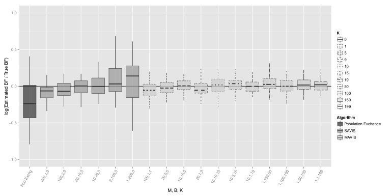
Figure 2: Box plots of the results of population exchange, SAVIS, and MAVIS on the Ising data.

We observe: improvements of the new methods over population exchange; an overall robustness of the new methods to different choices of parameters; and that there is a bias-variance tradeoff in the “internal” estimate of $Z(\widehat{\theta})/Z(\theta)$ in terms of producing the best behaviour of the Bayes’ factor estimates. Recall that as $B$ increases the bias of the internal estimate (the results of which can be observed in the results when using $B=0$) decreases, but for a fixed computational effort it is beneficial to use a lower $B$ and to instead increase $M$, using more importance points to decrease the variance. As in Alquier et al (2015), we observe that it may be useful to move away from the exact-approximate approaches, and in this case, to simply use the best available estimator of $Z(\widehat{\theta})/Z(\theta)$ (taking into account its statistical and computational efficiency) regardless of whether it is unbiased. In this example there is little observed difference in using our fixed computational budget on more AIS moves ($K$) in place of using more importance points ($M$). In general we might expect using more AIS moves to be more productive when the estimates of the $Z(\widehat{\theta})/Z(\theta)$ for $\theta$ far from $\widehat{\theta}$ are required.

2.6.2 $100\times 100$ Ising model

In this section we use SAVIS for estimating the marginal likelihood for a first order Ising model on data of size $100\times 100$ pixels simulated from an Ising model with parameter $\theta=10$. Again, estimating a marginal likelihood is done in three stages: firstly $\widehat{\theta}$ is estimated; followed by $Z(\widehat{\theta})$, then finally the marginal likelihood. The methods use for the first two stages are identical to those used in section 2.6.1, as is the choice of proposal distribution. The third stage is performed using SAVIS with $M=100$ and $B=20$. From 20 runs of this third stage, a five-number summary of the $\log$ evidence estimates was (-5790.251, -5790.178, -5790.144, -5790.119, -5790.009), with the average ESS being 80.75. Note the low variance over these runs of the algorithm and the high ESS, which were also found for different configurations of the algorithm (including for more importance points and larger values of $M$ and $B$). One might expect this example to be more difficult than the $10\times 10$ grids considered in the previous section, due to the need to find good estimates of $Z(\widehat{\theta})/Z(\theta)$ that are here normalising constants of distributions on a space of higher dimensions. However, since the posterior has lower variance in this case, only values of $\theta$ close to $\widehat{\theta}$ are proposed, which makes estimating $Z(\widehat{\theta})/Z(\theta)$ much easier, yielding the good results in this section.

2.7 Discussion

In this section we have compared the use of ABC-IS, SL-IS, MAVIS (and alternatives) for estimating marginal likelihoods and Bayes’ factors. The use of ABC for model comparison has received much attention, with much of the discussion centring around appropriate choices of summary statistics. We have avoided this in our examples by using exponential family models, but in general this remains an issue affecting both ABC and SL. It is the use of summary statistics that makes ABC and SL unable to provide evidence estimates. However, it is the use of summary statistics, usually essential in these settings, that provides ABC and SL with an advantage over MAVIS, in which importance sampling must be performed over the high dimensional data-space. Despite this disadvantage, MAVIS avoids the approximations made in the simulation based methods (illustrated in figures 1b to 1d, with the accuracy depending primarily on the quality of the estimate of $1/Z$ used). In section 2.6 we saw that there can be advantages of using biased, but lower variance estimates in place of standard IS.

The main weakness of all of the methods described in this section is that they are all based on standard IS and are thus not practical for use when $\theta$ is high dimensional. In the next section we examine the use of SMC samplers as an extension to IS for use on triply intractable problems, and in this framework discuss further the effect of inexact approximations.

3 Sequential Monte Carlo approaches

SMC samplers (Del Moral et al, 2006) are a generalisation of IS, in which the problem of choosing an appropriate proposal distribution in IS is avoided by performing IS sequentially on a sequence of target distributions, starting at a target that is easy to simulate from, and ending at the target of interest. In standard IS the number of Monte Carlo points required in order to obtain a particular accuracy increases exponentially with the dimension of the space, but Beskos et al (2011) show (under appropriate regularity conditions) that the use of SMC circumvents this problem and can thus be practically useful in high dimensions.

In this section we introduce SMC algorithms for simulating from doubly intractable posteriors which have the by-product that, like IS, they also produce estimates of marginal likelihoods. We note that, although here we focus on estimating the evidence, the SMC sampler approaches based here are a natural alternative to the MCMC methods described in section 1.1. and inherently use a “population” of Monte Carlo points (shown to be beneficial on these models by Caimo and Friel (2011)). In section 3.1 we describe these algorithms, before examining an application to estimating the precision matrix of a Gaussian distribution in high dimensions in section 3.2. In 3.4 we provide a preliminary investigation of the consequences of using biased weight estimates in an SMC framework.

3.1 SMC samplers in the presence of an INC

This section introduces two alternative SMC samplers for use on doubly intractable target distributions. The first, marginal SMC, directly follows from the IS methods in the previous section. The second, SMC-MCMC, requires a slightly different approach, but is more computationally efficient. Finally we briefly discuss simulation-based SMC samplers in section 3.1.2.

To begin, we introduce notation that is common to all algorithms that we discuss. SMC samplers perform sequential IS using $P$ “particles” $\theta^{(p)}$, each having (normalised) weight $w^{(p)}$, using a sequence of targets $\pi_{0}$ to $\pi_{T}$, with $\pi_{T}$ being the distribution of interest, in our case $\pi(\theta|y)\propto p(\theta)f(y|\theta)$. In this section we will take $\pi_{t}(\theta|y)\propto p(\theta)f_{t}(y|\theta)=p(\theta)\gamma_{t}(y|\theta)/Z_{t}(\theta)$. At target $t$, a “forward” kernel $K_{t}(\cdot|\theta_{t-1}^{(p)})$ is used to move particle $\theta_{t-1}^{(p)}$ to $\theta_{t}^{(p)}$, with each particle then being reweighted to give unnormalised weight

$$\widetilde{w}_{t}^{(p)} = \frac{p(\theta_{t}^{(p)})\gamma_{t}(y|\theta_{t}^{(p)})}{p(\theta_{t-1}^{(p)})\gamma_{t-1}(y|\theta_{t-1}^{(p)})}\frac{Z_{t-1}(\theta_{t-1}^{(p)})}{Z_{t}(\theta_{t}^{(p)})}\frac{L_{t-1}(\theta_{t}^{(p)},\theta_{t-1}^{(p)})}{K_{t}(\theta_{t-1}^{(p)},\theta_{t}^{(p)})}.$$

Here, $L_{t-1}$ represents a “backward” kernel that we chose differently in the alternative algorithms below. We note the presence of the INC, which means that this algorithm cannot be implemented in practice in its current form. The weights are then normalised to give $\left\{w_{t}^{(p)}\right\}$, and a resampling step is carried out. In the following sections the focus is on the reweighting step: this is the main difference between the different algorithms. For more detail on these methods, see Del Moral et al (2007).

Zhou et al (2015) describe how BFs can be estimated directly by SMC samplers, simply by taking $\pi_{1}$ to be one model and $\pi_{T}$ to be the other (with the $\pi_{t}$ being intermediate distributions). This idea is also explored for Gibbs random fields in Friel (2013). However, the empirical results in Zhou et al (2015) suggest that in some cases this method does not necessarily perform better than estimating marginal likelihoods for the two models separately and taking the ratio of the estimates. Here we do not investigate these algorithms further, but note that they offer an alternative to estimating the marginal likelihood separately.

3.1.1 Random weight SMC Samplers

SMC with an MCMC kernel

Suppose we were able to use a reversible MCMC kernel $K_{t}$ with invariant distribution $\pi_{t}(\theta|y)\propto p(\theta)f_{t}(y|\theta)$, and choose the $L_{t-1}$ kernel to be the time reversal of $K_{t}$ with respect to its invariant distribution, we obtain the following incremental weight:

$$\widetilde{w}_{t}^{(p)} = \frac{\gamma_{t}(y|\theta_{t-1}^{(p)})}{\gamma_{t-1}(y|\theta_{t-1}^{(p)})}\frac{Z_{t-1}(\theta_{t-1}^{(p)})}{Z_{t}(\theta_{t-1}^{(p)})}.$$ (12)

Once again, we cannot evaluate this incremental weight due to the presence of a ratio of normalising constants. Also, such an MCMC kernel cannot generally be directly constructed — the MH update itself involves evaluating the ratio of intractable normalising constants. However, appendix A shows that precisely the same weight update results when using either SAV or exchange MCMC moves in place of a direct MCMC step.

In order that this approach may be implemented we might consider, in the spirit of the approximations suggested in section 2, using an estimate of the ratio term $Z_{t-1}(\theta_{t-1}^{(p)})/Z_{t}(\theta_{t-1}^{(p)})$. For example, an unbiased IS estimate is given by

$$\widehat{\frac{Z_{t-1}(\theta_{t-1}^{(p)})}{Z_{t}(\theta_{t-1}^{(p)})}}=\frac{1}{M}\sum_{m=1}^{M}\frac{\gamma_{t-1}(u_{t}^{(m,p)}|\theta_{t-1}^{(p)})}{\gamma_{t}(u_{t}^{(m,p)}|\theta_{t-1}^{(p)})},$$ (13)

where $u_{t}^{(m,p)}\sim f_{t}(\cdot|\theta_{t-1}^{(p)})$. Although this estimate is unbiased, we note that the resultant algorithm does not have precisely the same extended space interpretation as the methods in Del Moral et al (2006). Appendix B gives an explicit construction for this case, which incorporates a pseudomarginal-type construction (Andrieu and Roberts, 2009).

Data point tempering

For the SMC approach to be efficient we require that the sequence of distributions $\{\pi_{t}\}$ be chosen such that $\pi_{0}$ is easy to simulate from, $\pi_{T}$ is the target of interest and the intermediate distributions provide a “route” between them. For the applications in this paper we found the data tempering approach of Chopin (2002) to be particularly useful. Suppose that the data $y$ consists of $N$ points, and that $N$ is exactly divisible by $T$ for ease of exposition. We then take $\pi_{0}(\theta|y)=p(\theta)$ and for $t=1,...T$ $\pi_{t}(\theta|y)=p(\theta)f_{t}(y|\theta)$ with

$$f_{t}(y|\theta)=f\left(y_{1:Nt/T}|\theta\right),$$ (14)

i.e. essentially we incorporate $N/T$ additional data points for each increment of $t$. On this sequence of targets we then propose to use the SMC sampler with an MCMC kernel as described in the previous section. The only slightly non-standard point is the estimation of $Z_{t-1}(\theta_{t-1}^{(p)})/$ $Z_{t}(\theta_{t-1}^{(p)})$, since in this case $Z_{t-1}(\theta_{t-1}^{(p)})$ and $Z_{t}(\theta_{t-1}^{(p)})$ are the normalising constants of distributions on different spaces. We use

$$\widehat{\frac{Z_{t-1}(\theta_{t-1}^{(p)})}{Z_{t}(\theta_{t-1}^{(p)})}}=\frac{1}{M}\sum_{m=1}^{M}\frac{\gamma_{t-1}(v_{t}^{(m,p)}|\theta_{t-1}^{(p)})q_{w}(w_{t}^{(m,p)})}{\gamma_{t}(u_{t}^{(m,p)}|\theta_{t-1}^{(p)})}$$ (15)

where $u_{t}^{(m,p)}\sim f_{t}(\cdot|\theta_{t-1}^{(p)})$ and $v_{t}^{(m,p)}$ and $w_{t}^{(m,p)}$ are subvectors of $u_{t}^{(m,p)}$. $w_{t}^{(m,p)}$ is in the space of the additional variables added when moving from $f_{t-1}$ to $f_{t}$ (providing the argument in an arbitrary auxiliary distribution $q_{w}(\cdot)$) and $v_{t}^{(m,p)}$ is in the space of the existing variables. For $t=1$ this becomes

$$\widehat{\frac{1}{Z_{1}(\theta_{0}^{(p)})}}=\frac{1}{M}\sum_{m=1}^{M}\frac{q_{w}(u_{1}^{(m,p)})}{\gamma_{1}(u_{1}^{(m,p)}|\theta_{0}^{(p)})}$$ (16)

with $u_{1}^{(m,p)}\sim f_{t}(.|\theta_{0}^{(p)})$.

Analogous to the SAV method, a sensible choice for $q_{w}(w)$ might be to use $f\left(w|\widehat{\theta}\right)$, where $w$ is on the same space as $N/T$ data points. The normalising constant for this distribution needs to be known to calculate the importance weight in (19) so, as earlier, we advocate estimating this in advance of running the SMC sampler (aside from when the data points are added one at a time - in this case the normalising constant may usually be found analytically). Note that if $y$ does not consist of i.i.d. points, it is useful to choose the order in which data points are added such that the same $q_{w}$ (each with the same normalising constant) can be used in every weight update. For example, in an Ising model, the requirement would be to add the same shape grid of variables at each target.

Marginal SMC

An alternative method commonly used in ABC applications arises from the use of an approximation to the optimal backward kernel (Peters, 2005; Klaas et al, 2005). In this case the weight update is

$$\widetilde{w}_{t}^{(p)} = \frac{p(\theta_{t}^{(p)})\gamma_{t}(y|\theta_{t}^{(p)})}{Z_{t}(\theta_{t}^{(p)})\sum_{r=1}^{P}w_{t-1}^{(r)}K_{t}(\theta_{t}^{(p)}|\theta_{t-1}^{(r)})}$$ (17)

for an arbitrary forward kernel $K_{t}$. This results in a computational complexity of $O(P^{2})$ compared to $O(P)$ for a standard SMC method, but we include it here in order to note that the $1/Z(\cdot)$ term in (17) could be dealt with in the same way as in the simple IS case. Considering the SAVM posterior, where in target $t$ we use the distribution $q_{u}$ for the auxiliary variable $u_{t}$, and the SAVM proposal, where $u_{t}^{(p)}\sim f_{t}(\cdot|\theta_{t}^{(p)})$ we arrive at the weight update:

$$\widetilde{w}_{t}^{(p)} = \frac{q_{u}(u_{t}^{(p)}|\theta_{t}^{(p)},y)p(\theta_{t}^{(p)})\gamma_{t}(y|\theta_{t}^{(p)})}{\gamma_{t}(u_{t}^{(p)}|\theta_{t}^{(p)})\sum_{r=1}^{P}w_{t-1}^{(r)}K_{t}(\theta_{t}^{(p)}|\theta_{t-1}^{(r)})}.$$

in which normalising constant appears in this weight update. We include this approach for completeness but do not investigate it further in this paper.

3.1.2 Simulation-based SMC samplers

Section 2.2 describes how the ABC and SL approximations may be used within IS. The same approximate likelihoods may be used in SMC. In ABC (Sisson et al, 2007), where the sequence of targets is chosen to be $\pi_{t}(\theta)\propto p(\theta)\widehat{f}_{\epsilon_{t}}(y|\theta)$ with a decreasing sequence $\epsilon_{t}$, this idea provides a useful alternative to MCMC for exploring ABC posterior distributions, whilst also providing estimates of Bayes’ factors (Didelot et al, 2011). The use of SMC with SL does not appear to have been explored previously. One might expect SMC to be useful in this context (using, for example, the sequence of targets $\pi_{t}(\theta)\propto p(\theta)\widehat{f}_{\mbox{SL}}^{(t/T)}\left(S(y)|\theta\right)$), particularly when $\widehat{f}_{\mbox{SL}}$ is concentrated relative to the prior.

3.2 Application to precision matrices

In this section we examine the performance of the SMC sampler, with MCMC proposal and data-tempered target distributions, for estimating the evidence in an example in which $\theta$ is of moderately high dimension. We consider the case in which $\theta=\Sigma^{-1}$ is an unknown precision matrix, $f(y|\theta)$ is the $d$-dimensional multivariate Gaussian distribution with zero mean and $p(\theta)$ is a Wishart distribution $\mathcal{W}(\nu,V)$ with parameters $\nu\geq d$ and $V\in\mathbb{R}^{d\times d}$. Suppose we observe $n$ i.i.d. observations $y=\left\{y_{i}\right\}_{i=1}^{n}$, where $y_{i}\in\mathbb{R}^{d}$. The true evidence can be calculated analytically, and is given by

$$p(y)=\frac{1}{\pi{}^{nd/2}}\frac{\Gamma_{d}(\frac{\nu+n}{2})}{\Gamma_{d}(\frac{\nu}{2})}\frac{\left|\left(V^{-1}+\sum_{i=1}^{n}y_{i}y_{i}^{T}\right)^{-1}\right|^{\frac{\nu+n}{2}}}{\left|V\right|^{\frac{\nu}{2}}},$$ (18)

where $\Gamma_{d}$ denotes the $d$-dimensional gamma function. For ease of implementation, we parametrise the precision using a Cholesky decomposition $\Sigma^{-1}=LL^{\prime}$ with $L$ a lower triangular matrix whose $(i,j)$’th element is denoted $a_{ij}$.

As in section 2.3, we write $f(y|\theta)$ as $\gamma(y|\theta)/Z(\theta)$ as follows

$$f\left(\left\{y_{i}\right\}_{i=1}^{n}\mid\Sigma^{-1}\right) = \left|2\pi\Sigma\right|^{-n/2}\exp\left(-\frac{1}{2}\sum_{i=1}^{n}y_{i}^{\prime}\Sigma^{-1}y_{i}\right),$$

where in some of the experiments that follow, $Z(\theta)=\left|2\pi\Sigma\right|^{n/2}$ is treated as if it is an INC. In the Wishart prior, we take $\nu=10+d$ and $V=I_{d}$.

Taking $d=10$, $n=30$ points were simulated using $y_{i}\sim\mathcal{MVN}\left(0_{d},0.1\times I_{d}\right)$. The parameter space is thus 55-dimensional, motivating the use of an SMC sampler in place of IS or the population exchange method, neither of which are suited to this problem. In the SMC sampler, in which we used $P=10,000$ particles, the sequence of targets is given by data point tempering. Specifically, the sequence of targets is to use $p(\Sigma^{-1})$ when $t=0$ and $p(\Sigma^{-1})f\left(\left\{y_{i}\right\}_{i=1}^{t}\mid\Sigma^{-1}\right)$ for $t=1,...,T$ (with $T=n$). The parameters are $\left\{a_{ij}\mid 1\leq j\leq i\leq d\right\}$. We use single component MH kernels to update each of the parameters, with one (deterministic) sweep consisting of an update of each in turn. For each $a_{ij}$ we use a Gaussian random walk proposal, where at target $t$, the variance for the proposal used for $a_{ij}$ is taken to be the sample variance of $a_{ij}$ at target $t-1$. For updating the weights of each particle we used equation 15, where we chose $q_{w}(\cdot)=f\left(\cdot\mid\widehat{\Sigma^{-1}}\right)$ with $\widehat{\Sigma^{-1}}$ the maximum likelihood estimate of the precision $\Sigma^{-1}$, and chose $M=200$ “internal” importance sampling points. Systematic resampling was performed when the effective sample size (ESS) fell below $P/2$.

We estimated the evidence 10 times using the SMC sampler and compared the statistical properties of each algorithm using these estimates. For our simulated data, the $\log$ of the true evidence was $-89.43$. Over the 10 runs of the SMC sampler a five-number summary of the $\log$ evidence estimates was ($-90.01$, $-89.51$, $-89.35$, $-88.92$, $-88.37$).

3.3 Application to Ising models

In this section we apply the random weight SMC sampler to the Ising model data considered in section 2.6.1. We use SMC to estimate the marginal likelihood of both the first and second order Ising models, then take the ratio of these estimates to estimate the Bayes’ factor. Note that in this case the size of the parameter space is much smaller than in the precision example, with the models having parameter spaces of sizes 1 and 2 respectively. The excellent results achieved by IS in section 2.6.1 might seem to imply that SMC samplers are not required for this problem, but recall that we required preliminary runs of the exchange algorithm in order to design an appropriate importance proposal, along with an SMC sampler in order to estimate the normalising constant $Z(\widehat{\theta})$ of the distribution $q_{u}$ used for the auxiliary variables $u^{(m)}$. An SMC sampler offers a cleaner approach that requires less user tuning.

We applied the random weight SMC sampler described in section 3.1.1, with 500 particles, data point tempering (adding one pixel at a time, taking $q_{w}$ to be $\mbox{Bern}(0.5)$), and using the estimate of the ratio of normalising constants in the weight update from equation (15) with $M=20$ importance points. Each of these estimates requires simulating a single point from $\gamma_{t}(\cdot|\theta_{t-1}^{(p)})$ using a Gibbs sampler, which had a burn in of $B=10$ iterations, yielding a total computational budget of 200 Gibbs sweeps for estimating the ratio of normalising constants. Note that, as considered in section 2.6.1, this use of a Gibbs sampler results in an inexact algorithm, but this level of burn in was found to be sufficient for this bias to be minimal in the random weight IS algorithms. The MCMC kernel of the exchange algorithm was used (with proposal taken to be the sample variance of the set of particles at each SMC iteration), using the approximate version where a Gibbs sampler with burn in $B=10$ iterations is used to simulate from $\gamma_{t}(\cdot|\theta^{(*)})$. The total cost of this algorithm is comparable to the IS approaches in section 2.6.1, with a total cost of $5.25\times 10^{6}$ Gibbs sweeps and hence around a quarter of that of the algorithm of Friel (2013). Figure 3 shows the results produced by this method in comparison with those from Friel (2013).

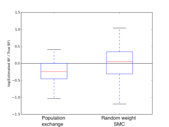
Figure 3: Box plots of the results of population exchange and random weight SMC.

We observe that the median of the random weight SMC estimates is more accurate than that of the population exchange estimates - the bias introduced through using an internal Gibbs sampler in place of an exact sampler does not appear to accumulate sufficiently to affect the results (this issue is explored further in the following section). However, it has slightly higher variance than population exchange (much higher than SAVIS and MAVIS). This high variance can be attributed to two factors:

1. Since the SMC sampler begins with points sampled from the prior, larger changes in $\theta$ are considered than in the IS approaches, thus the estimates of the ratio of the normalising constants require more importance points to be accurate - the results suggest that the budget of 200 Gibbs sweeps is insufficient. This is the opposite situation to that encountered in section 2.6.2, where the changes in $\theta$ are small and the estimates of the ratio of the normalising constants are accurate with small numbers of importance points.

2. It’s been frequently observed (cf. Lee and Whiteley (2015)) that, as suggested by the asymptotic variance expansion, in some instances the first few iterations of an SMC sampler contribute substantially to the ultimate error. This issue arises since the forgetting of the sampler doesn’t suppress the terms that the initial errors contribute to the asymptotic variance enough to compensate for the fact that they’re much larger than the final ones. This is due, when using data point tempering in the manner we have here, to the much larger relative discrepancy between the first few distributions in the sequence than between later distributions.

We conclude that the random weight SMC method is a viable approach to estimating Bayes’ factors for these models, but that care should be taken in tuning the weight estimates and choosing the sequence of SMC distributions.

3.4 Biased Weights in SMC

3.4.1 Error bounds

We now examine the effect of using inexact weights on estimates produced by SMC samplers. By way of theoretical motivation of such an approach, we demonstrate that under strong, but standard (cf. Del Moral (2004)), assumptions on the mixing of the sampler, if the approximation error is sufficiently small, then this error can be controlled uniformly over the iterations of the algorithm and will not accumulate unboundedly over time (and that it can in principle be made arbitrarily small by making the relative bias small enough for the desired level of accuracy). We do not here consider the particle system itself, but rather the sequence of distributions which are being approximated by Monte Carlo in the approximate version of the algorithm and in the idealised algorithm being approximated. The Monte Carlo approximation of this sequence can then be understood as a simple mean field approximation and its convergence has been well studied, see for example Del Moral (2004).

In order to do this, we make a number of identifications in order to allow the consideration of the approximation in an abstract manner. We allow $\widetilde{G}_{t}$ to denote the incremental weight function at time $t$, and $G_{t}$ to denote the exact weight function which it approximates (any auxiliary random variables needed in order to obtain this approximation are simply added to the state space and their sampling distribution to the transition kernel). The transition kernel $M_{t}$ combines the proposal distribution of the SMC algorithm together with the sampling distribution of any needed auxiliary variables. We allow $x$ to denote the full collection of variables sampled during an iteration of the sampler, which is assumed to exist on the same space during each iteration of the sampler.

We employ the following assumptions (we assume an infinite sequence of algorithm steps and associated target distributions, proposals and importance weights; naturally, in practice only a finite number would be employed but this formalism allows for a straightforward statement of the result):

A1

(Bounded Relative Approximation Error) There exists $\gamma<\infty$ such that:

$$\sup_{t\in\mathbb{N}}\sup_{x}\frac{|G_{t}(x)-\widetilde{G}_{t}(x)|}{\widetilde{G}_{t}(x)}\leq\gamma.$$

A2

(Strong Mixing; slightly stronger than a global Doeblin condition) There exists $\epsilon(M)>0$ such that:

$$\sup_{t\in\mathbb{{N}}}\inf_{x,y}\frac{dM_{t}(x,\cdot)}{dM_{t}(y,\cdot)}\geq\epsilon(M).$$

A3

(Control of Potential) There exists $\epsilon(G)>0$ such that:

$$\sup_{t\in\mathbb{{N}}}\inf_{x,y}\frac{G_{t}(x)}{G_{t}(y)}\geq\epsilon(G).$$

The first of these assumptions controls the error introduced by employing an inexact weighting function; the others ensure that the underlying dynamic system is sufficiently ergodic to forget it’s initial conditions and hence limit the accumulation of errors. We demonstrate below that the combination of these properties suffices to transfer that stability to the approximating system.

We consider the behaviour of the distributions $\eta_{p}$ and $\tilde{\eta}_{p}$ which correspond to the target distributions at iteration $p$ of the exact and approximating algorithms, prior to reweighting, at iteration $p$ in the following proposition, the proof of which is provided in Appendix C, which demonstrates that if the approximation error, $\gamma$, is sufficiently small then the accumulation of error over time is controlled:

Proposition 1 (Uniform Bound on Total-Variation Discrepancy).

If A1, A2 and A3 hold then:

$$\sup_{n\in\mathbb{N}}\left\|\eta_{n}-\widetilde{\eta}_{n}\right\|_{\mbox{TV}}\leq\frac{4\gamma(1-\epsilon(M))}{\epsilon^{3}(M)\epsilon(G)}.$$

This result is not intended to do any more than demonstrate that, qualitatively, such forgetting can prevent the accumulation of error even in systems with “biased” importance weighting potentials. In practice, one would wish to make use of more sophisticated ergodicity results such as those of Whiteley (2013), within this framework to obtain results which are somewhat more broadly applicable: assumptions A2 and A3 are very strong, and are used only because they allow stability to be established simply. Although this result is, in isolation, too weak to justify the use of the approximation schemes introduced here in practice, together with the empirical results presented below, it does suggest that further investigation of such approximations is warranted particularly in settings in which unbiased estimators are not available.

3.4.2 Empirical results

We use the precision example introduced in section 3.2 to investigate the effect of using biased weights in SMC samplers. Specifically we take $d=1$ and use a simulated dataset $y$ where $n=5000$ points were simulated using $y_{i}\sim\mathcal{N}\left(0,0.1\right)$. In this case there is only a single parameter to estimate, $a_{1}$, and we examine the bias of estimates of the evidence using four alternative SMC samplers, each of which use a data-tempered sequence of targets (adding one data point at each target). For this data we can calculate analytically the true value of the marginal likelihood after receiving each data point, thus we can estimate the bias of each sampler at each iteration. The first SMC sampler (the “exact weight” sampler) is the method where the true value of $Z_{t-1}(\theta_{t-1}^{(p)})/Z_{t}(\theta_{t-1}^{(p)})$ is used in the weight update. The second is the same “unbiased random weight” sampler used in section 3.2, which uses an unbiased IS weight estimate, here with $M=20$ “internal” importance sampling points. The third, which we refer to as the “biased random weight” sampler, uses a biased bridge estimator instead, specifically we use in place of (15)

$$\widehat{\frac{Z_{t-1}(\theta_{t-1}^{(p)})}{Z_{t}(\theta_{t-1}^{(p)})}}=\left(\sum_{m=1}^{M/2}\left[\frac{\gamma_{t-1}(v_{t,1}^{(m,p)}|\theta_{t-1}^{(p)})q_{w}(w_{t,1}^{(m,p)})}{\gamma_{t}(u_{t,1}^{(m,p)}|\theta_{t-1}^{(p)})}\right]^{1/2}\right)\left/\right.$$

$$\qquad\left(\sum_{m=1}^{M/2}\left[\frac{\gamma_{t}(u_{t,2}^{(m,p)}|\theta_{t-1}^{(p)})}{\gamma_{t-1}(v_{t,2}^{(m,p)}|\theta_{t-1}^{(p)})q_{w}(w_{t,2}^{(m,p)})}\right]^{1/2}\right),$$ (19)

where $v_{t,2}^{(m,p)}\sim f_{t-1}(.|\theta_{t-1}^{(p)})$, $w_{t,2}^{(m,p)}\sim q_{w}(.)$ so that $u_{t,2}^{(m,p)}=\left(v_{t,2}^{(m,p)},w_{t,2}^{(m,p)}\right)$, and $u_{t,1}^{(m,p)}\sim f_{t}(.|\theta_{t-1}^{(p)})$ with $v_{t,1}^{(m,p)}$ and $w_{t,1}^{(m,p)}$ being the corresponding subvectors of $u_{t,1}^{(m,p)}$.

Motivated by the theoretical argument presented previously, we investigate the effect of improving the mixing of the kernel used within the SMC. In this model the exact posterior is available at each SMC target, so we may replace the use of an MCMC move to update the parameter with a direct simulation from the posterior. In this extreme case, there is no dependence between each particle and its history; we refer to this, the fourth SMC sampler we consider, as “biased random weight with perfect mixing”. Each SMC sampler was run 20 times, using 50 particles.

Figures 4 and 5 show the estimated bias and mean square error of the $\log$ evidence estimates of each sampler at each iteration. No bias is observed in the algorithm with true weights, and only a small bias is observed in the unbiased random weight sampler (this bias is likely to be due to the relatively small number of replications). Bias does accumulate in the biased random weight sampler, but we note that the level of bias appears to stabilise. This accumulation of bias means that one should exercise caution in the use of SMC samplers with biased weights. However, we observe that perfect mixing substantially decreases the bias in the evidence estimates from the algorithm. Also, in this case we observe that the bias does not accumulate sufficiently to give poor estimates of the evidence. Here the standard deviation of the final $\log$ evidence estimate over the random weight SMC sampler runs is approximately 0.4, so the bias is not large by comparison.

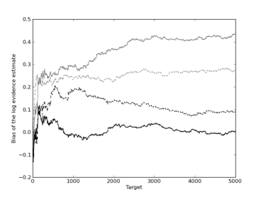
Figure 4: The estimated bias in the $\log$ evidence estimates of the true (black solid), unbiased random weight (black dashed), biased random weight (grey solid) SMC algorithms using MCMC kernels, and the estimated bias when using the biased random weight algorithm with perfect mixing (grey dashed).

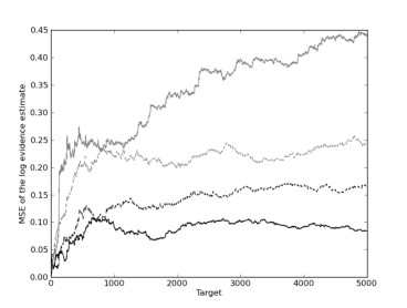
Figure 5: The estimated MSE in the $\log$ evidence estimates of the four SMC samplers (same key as figure 4).

3.5 Discussion

In section 2.6 we observed clearly that the use of biased weights in IS can be useful for estimating the evidence in doubly intractable models, but we have not observed the same for SMC with biased weights. When applied to the precision example in section 3.2, an inexact sampler (using the bridge estimator) did not outperform the exact sampler, despite the mean square error of the biased bridge weight estimates being substantially improved compared to the unbiased IS estimate. Over 10 runs the mean square error in the $\log$ evidence was 0.34 for the inexact sampler, compared to 0.28 for the exact sampler. This experience suggests that samplers with biased weights should be used with caution: weight estimates with low variance do not guarantee good performance due to the accumulation of bias in the SMC.

However, the theoretical and empirical investigation in this section suggests that this idea is worth further investigation, possibly for situations involving some of the other intractable likelihoods listed in section 1. Our results suggest that improved mixing can help combat the accumulation of bias, which may imply that there may be situations where it is useful to perform many iterations of a kernel at a particular target, rather than the more standard approach of using many intermediate targets at each of which a single iteration of a kernel is used. Other variations are also possible, such as the calculation of fast cheap biased weights at each target in order only to adaptively decide when to resample, with more accurate weight estimates (to ensure accurate resampling and accurate estimates based on the particles) only calculated when the method chooses to resample.

4 Conclusions

This paper describes several IS and SMC approaches for estimating the evidence in models with INCs that outperform previously described approaches. These methods may also prove to be useful alternatives to MCMC for parameter estimation. Several of the ideas in the paper are also applicable more generally, in particular the use of synthetic likelihood in the IS context and the notion of using biased weight estimates in IS and SMC. We note that the bias in these biased weight methods may be small compared to errors resulting from commonly accepted approximate techniques such as ABC.

For biased IS, in section 2.5 we show that the error of estimates from low-variance biased methods can be less than those from unbiased methods of higher variance. This is comparable to a result for biased MCMC methods (Johndrow et al, 2015), where it is shown that the error of estimates from a computationally cheap biased MCMC can be less than those from an expensive exact MCMC. In both cases, given a finite computational budget, it is not always the case that this budget should be spent on guaranteeing the exactness of the sampler if minimizing approximation error is the objective.

A similar choice concerning the allocation of computational resources arises in SMC. Here, one does need to be especially careful about the use of biased SMC, due to the possible accumulation of bias over SMC iterations. One might expect this accumulated bias to outweigh any benefits a reduced variance may bring. For this reason we advise caution in the use of biased SMC in general. This paper does, however, indicate that there may exist cases where biased SMC is useful, through: the theoretical result that under strong mixing conditions bias does not accumulate unboundedly; the empirical evidence that fast mixing may reduce the accumulation of bias; and the empirical results where we observe (in a situation where the distance between successive targets decreases) that the rate at which bias accumulates decreases with time.

Appendix A Using SAV and exchange MCMC within SMC

A.1 Weight update when using SAV-MCMC

Let us consider the SAVM posterior, with $K$ being the MCMC move used in SAVM. In this case the weight update is

$$\widetilde{w}_{k}^{(p)} = \frac{p(\theta_{t}^{(p)})f_{t}(y|\theta_{t}^{(p)})q_{u}(u_{t}^{(p)}|\theta_{t}^{(p)},y)}{p(\theta_{t-1}^{(p)})f_{t-1}(y|\theta_{t-1}^{(p)})q_{u}(u_{t-1}^{(p)}|\theta_{t-1}^{(p)},y)}$$

$$\qquad\frac{L_{t-1}((\theta_{t}^{(p)},u_{t}^{(p)}),(\theta_{t-1}^{(p)},u_{t-1}^{(p)}))}{K_{t}((\theta_{t-1}^{(p)},u_{t-1}^{(p)}),(\theta_{t}^{(p)},u_{t}^{(p)}))}$$

$$= \frac{p(\theta_{t}^{(p)})f_{t}(y|\theta_{t}^{(p)})q_{u}(u_{t}^{(p)}|\theta_{t}^{(p)},y)}{p(\theta_{t-1}^{(p)})f_{t-1}(y|\theta_{t-1}^{(p)})q_{u}(u_{t-1}^{(p)}|\theta_{t-1}^{(p)},y)}$$

$$\qquad\frac{p(\theta_{t-1}^{(p)})f_{t}(y|\theta_{t-1}^{(p)})q_{u}(u_{t-1}^{(p)}|\theta_{t-1}^{(p)},y)}{p(\theta_{t}^{(p)})f_{t}(y|\theta_{t}^{(p)})q_{u}(u_{t}^{(p)}|\theta_{t}^{(p)},y)}$$

$$= \frac{\gamma_{t}(y|\theta_{t-1}^{(p)})}{\gamma_{t-1}(y|\theta_{t-1}^{(p)})}\frac{Z_{t-1}(\theta_{t-1}^{(p)})}{Z_{t}(\theta_{t-1}^{(p)})},$$

which is the same update as if we could use MCMC directly.

A.2 Weight update when using the exchange algorithm

Nicholls et al (2012) show the exchange algorithm, when set up to target $\pi_{t}(\theta|y)\propto p(\theta)f_{t}(y|\theta)$ in the manner described in section 1.1.2, simulates a transition kernel that is in detailed balance with $\pi_{t}(\theta|y)$. This follows from showing that it satisfies a “very detailed balance” condition, which takes account of the auxiliary variable $u$. The result is that the derivation of the weight update follows exactly that of (12).

Appendix B An extended space construction for the random weight SMC method in section 3.1.1

The following extended space construction justifies the use of the “approximate” weights in (13) via an explicit sequential importance (re)sampling argument along the lines of Del Moral et al (2006), albeit with a slightly different sequence of target distributions.

Consider an actual sequence of target distributions $\{\pi_{t}\}_{t\geq 0}$. Assume we seek to approximate a normalising constant during every iteration by introducing additional variables $u_{t}=(u_{t}^{1},\ldots,u_{t}^{M})$ during iteration $t>0$.

Define the sequence of target distributions:

$$\widetilde{\pi}_{t}\left(\widetilde{x}_{t}=(\theta_{0},\theta_{1},u_{1},\ldots,\theta_{t},u_{t})\right)$$

$$:= \pi_{t}(\theta_{t})\prod_{s=0}^{t-1}L_{s}(\theta_{s+1},\theta_{s})\cdot$$

$$\phantom{\pi_{t}(\theta_{t})}\prod_{s=1}^{t}\frac{1}{M}\sum_{m=1}^{M}\left[f_{s-1}(u_{s}^{m}|\theta_{s-1})\prod_{q\neq m}f_{s}(u_{s}^{m}|\theta_{s-1})\right]$$

where $L_{s}$ has the same rôle and interpretation as it does in a standard SMC sampler.

Assume that at iteration $t$ the auxiliary variables $u_{t}^{m}$ are sampled independently (conditional upon the associated value of the parameter, $\theta_{t-1}$)and identically according to $f_{t}(\cdot|\theta_{t-1})$ and that $K_{t}$ denotes the incremental proposal distribution at iteration $t$, just as in a standard SMC sampler.

In the absence of resampling, each particle has been sampled from the following proposal distribution at time $t$:

$$\widetilde{\mu}_{t}(\widetilde{x}_{t})= \mu_{0}(\theta_{0})\prod_{s=1}^{t}K_{s}(\theta_{s-1},\theta_{s})\prod_{s=1}^{t}\prod_{m=1}^{M}f_{s}(u_{s}^{m}|\theta_{s-1})$$

and hence its importance weight, $W_{t}(\widetilde{x}_{t})$, should be:

$$\frac{\pi_{t}(\theta_{t})\prod_{s=0}^{t-1}L_{s}(\theta_{s+1},\theta_{s})}{\mu_{0}(\theta_{0})\prod_{s=1}^{t}K_{s}(\theta_{s-1},\theta_{s})}$$

$$\frac{\prod_{s=1}^{t}\frac{1}{M}\sum_{m=1}^{M}\left[f_{s-1}(u_{s}^{m}|\theta_{s-1})\prod_{q\neq m}f_{s}(u_{s}^{m}|\theta_{s-1})\right]}{\prod_{s=1}^{t}\prod_{m=1}^{M}f_{s}(u_{s}^{m}|\theta_{s-1})}$$

$$= \frac{\pi_{t}(\theta_{t})\prod_{s=0}^{t-1}L_{s}(\theta_{s+1},\theta_{s})}{\mu_{0}(\theta_{0})\prod_{s=1}^{t}K_{s}(\theta_{s-1},\theta_{s})}\prod_{s=1}^{t}\frac{1}{M}\sum_{m=1}^{M}\frac{f_{s-1}(u_{s}^{m}|\theta_{s-1})}{f_{s}(u_{s}^{m}|\theta_{s-1})}$$

$$= W_{t-1}(\widetilde{x}_{t-1})\cdot\frac{\pi_{t}(\theta_{t})L_{t-1}(\theta_{t},\theta_{t-1})}{\pi_{t-1}(\theta_{t-1})K_{t}(\theta_{t-1},\theta_{t})}$$

$$\qquad\frac{1}{M}\sum_{m=1}^{M}\frac{f_{t-1}(u_{t}^{m},\theta_{t-1})}{f_{t}(u_{t}^{m}|\theta_{t-1})},$$

which yields the natural sequential importance sampling interpretation. The validity of the incorporation of resampling follows by standard arguments.

If one has that $\pi_{t}(\theta_{t})\propto p(\theta_{t})f_{t}(y|\theta_{t})=p(\theta_{t})\gamma_{t}(y|\theta_{t})/Z_{t}(\theta_{t})$ and employs the time reversal of $K_{t}$ for $L_{t-1}$ then one arrives at an incremental importance weight, at time $t$ of:

$$\frac{p(\theta_{t})f_{t}(y|\theta_{t-1})}{p(\theta_{t-1})f_{t-1}(y|\theta_{t-1})}\frac{1}{M}\sum_{m=1}^{M}\frac{f_{t-1}(u_{t}^{m}|\theta_{t-1})}{f_{t}(u_{t}^{m}|\theta_{t-1})}=$$

$$\qquad\frac{p(\theta_{t})\gamma_{t}(y|\theta_{t-1})}{p(\theta_{t-1})\gamma_{t-1}(y|\theta_{t-1})}\frac{1}{M}\sum_{m=1}^{M}\frac{\gamma_{t-1}(u_{t}^{m}|\theta_{t-1})}{\gamma_{t}(u_{t}^{m}|\theta_{t-1})}$$

yielding the algorithm described in section 3.1.1 as an exact SMC algorithm on the described extended space.

Appendix C Proof of SMC Sampler Error Bound

A little notation is required. We allow $(E,\mathcal{E})$ to denote the common state space of the sampler during each iteration, $\mathcal{C}_{b}(E)$ the collection of continuous, bounded functions from $E$ to $\mathbb{R}$, and $\mathcal{P}(E)$ the collection of probability measures on this space. We define the Boltzmann-Gibbs operator associated with a potential function $G:E\to(0,\infty)$ as a mapping, $\Psi_{G}:\mathcal{P}(E)\rightarrow\mathcal{P}(E)$, weakly via the integrals of any function $\varphi\in\mathcal{C}_{b}(E)$

$$\int\varphi(x)\Psi_{G}(\eta)(dx)=\frac{\int\eta(dx)G(x)\varphi(x)}{\int\eta(dx^{\prime})G(x^{\prime})}.$$

The integral of a set $A$ under a probability measure $\eta$ is written $\eta(A)$ and the expectation of a function $\varphi$ of $X\sim\eta$ is written $\eta(\varphi)$. The supremum norm on $\mathcal{C}_{b}(E)$ is defined $||\varphi||_{\infty}=\sup_{x\in E}\varphi(x)$ and the total variation distance on $\mathcal{P}(E)$ is $||\mu-\nu||_{\text{TV}}=\sup_{A}(\nu(A)-\mu(A))$. Markov kernels, $M:E\rightarrow\mathcal{P}(E)$ induce two operators, one on integrable functions and the other on (probability) measures:

$$\forall\varphi\in \mathcal{C}_{b}(E): M(\varphi)(\cdot):= \int M(\cdot,dy)\varphi(y)$$

$$\forall\mu\in \mathcal{P}(E): (\mu M)(\cdot):= \int\mu(dx)M(x,\cdot).$$

Having established this notation, we note that we have the following recursive definition of the distributions we consider:

$$\widetilde{\eta}_{0}= \eta_{0}=:M_{0} {\eta}_{t\geq 1}= \Psi_{G_{t-1}}(\eta_{t-1}) \widetilde{\eta}_{t\geq 1}= \Psi_{\widetilde{G}_{t-1}}(\widetilde{\eta}_{t-1})$$

and for notational convenience define the transition operators as

$$\Phi_{t}(\eta_{t-1})= \Psi_{G_{t-1}}(\eta_{t-1})M_{t} \widetilde{\Phi}_{t}(\widetilde{\eta}_{t-1})= \Psi_{\widetilde{G}_{t-1}}(\widetilde{\eta}_{t-1})M_{t}.$$

We make use of the (nonlinear) dynamic semigroupoid, which we define recursively, via it’s action on a generic probability measure $\eta$, for $t\in\mathbb{N}$:

$$\Phi_{t-1,t}(\eta)= \Phi_{t}(\eta) \Phi_{s,t}=\Phi_{t}(\Phi_{s,t-1}(\eta))\text{ for }s<t,$$

with $\Phi_{t,t}(\eta)=\eta$ and $\widetilde{\Phi}_{s,t}$ defined correspondingly.

We begin with a lemma which allows us to control the discrepancy introduced by Bayesian updating of a measure with two different likelihood functions.

Lemma 1 (Approximation Error).

If A1. holds, then $\forall\eta\in\mathcal{P}(E)$ and any $t\in\mathbb{N}$:

$$||\Psi_{\widetilde{G}_{t}}(\eta)-\Psi_{G_{t}}(\eta)||_{TV}\leq 2\gamma.$$

Proof.

Let $\Delta_{t}:=\widetilde{G}_{t}-G_{t}$ and consider a generic $\varphi\in\mathcal{C}_{b}(E)$:

$$(\Psi_{\widetilde{G}_{t}}(\eta)-\Psi_{G_{t}}(\eta))(\varphi)$$

$$= \frac{\eta(G_{t})\eta(\widetilde{G}_{t}\varphi)-\eta(\widetilde{G}_{t})\eta(G_{t}\varphi)}{\eta(\widetilde{G}_{t})\eta(G_{t})}$$

$$= \frac{\eta(G_{t})\eta((G_{t}+\Delta_{t})\varphi)-\eta((G_{t}+\Delta_{t}))\eta(G_{t}\varphi)}{\eta(\widetilde{G}_{t})\eta(G_{t})}$$

$$= \frac{\eta(G_{t})\eta(\Delta_{t}\varphi)-\eta(\Delta_{t})\eta(G_{t}\varphi)}{\eta(\widetilde{G}_{t})\eta(G_{t})}$$

Considering the absolute value of this discrepancy, making using of the triangle inequality:

$$\left|(\Psi_{\widetilde{G}_{t}}(\eta)-\Psi_{G_{t}}(\eta))(\varphi)\right|\leq \left|\frac{\eta(\Delta_{t}\varphi)}{\eta(\widetilde{G}_{t})}\right|+\left|\frac{\eta(\Delta_{t})}{\eta(\widetilde{G}_{t})}\right|\left|\frac{\eta(G_{t}\varphi)}{\eta(G_{t})}\right|$$

Noting that $G_{t}$ is strictly positive, we can bound $|\eta(G_{t}\varphi)|/\eta(G_{t})$ with $\eta(G_{t}|\varphi|)/\eta(G_{t})$ and thus with $\left\|\varphi\right\|_{\infty}$ and apply a similar strategy to the first term:

$$\left|(\Psi_{\widetilde{G}_{t}}(\eta)-\Psi_{G_{t}}(\eta))(\varphi)\right|$$

$$\leq \left|\frac{\eta(|\Delta_{t}|)\left\|\varphi\right\|_{\infty}}{\eta(\widetilde{G}_{t})}\right|+\left|\frac{\eta(\Delta_{t})}{\eta(\widetilde{G}_{t})}\right|\left|\frac{\eta(G_{t}|\varphi|)}{\eta(G_{t})}\right|\leq 2\gamma\left\|\varphi\right\|_{\infty}.$$

(noting that $\eta(|\Delta_{t}|)/\eta(\widetilde{G_{t}})<\gamma$ by integration of both sides of A1). ∎

We now demonstrate that, if the local approximation error at each iteration of the algorithm(characterised by $\gamma$) is sufficiently small then it does not accumulate unboundedly as the algorithm progresses.

Proof of Proposition 1.

We begin with a telescopic decomposition (mirroring the strategy employed for analysing particle approximations of these systems in Del Moral (2004)):

$$\eta_{t}-\widetilde{\eta}_{t}= \sum_{s=1}^{t}\Phi_{s-1,t}(\widetilde{\eta}_{s-1})-\Phi_{s,t}(\widetilde{\eta}_{s}).$$

We thus establish (noting that $\widetilde{\eta}_{0}=\eta_{0}$):

$$\eta_{t}-\widetilde{\eta}_{t}= \sum_{s=1}^{t}\Phi_{s,t}(\Phi_{s}(\widetilde{\eta}_{s-1}))-\Phi_{s,t}(\widetilde{\Phi}_{s}(\widetilde{\eta}_{s-1})).$$ (20)

Turning our attention to an individual term in this expansion, noting that:

$$\Phi_{s}(\eta)(\varphi)= \Psi_{G_{s-1}}(\eta)M_{s}(\varphi) \widetilde{\Phi}_{s}(\eta)(\varphi)= \Psi_{\widetilde{G}_{s-1}}(\eta)M_{s}(\varphi)$$

we have, by application of a standard Dobrushin contraction argument and Lemma 1

$$(\Phi_{s}(\widetilde{\eta}_{s-1})-\widetilde{\Phi}_{s}(\widetilde{\eta}_{s-1}))(\varphi)$$ (21)

$$= \Psi_{G_{s-1}}(\widetilde{\eta}_{s-1})M_{s}(\varphi)-\Psi_{\widetilde{G}_{s-1}}(\widetilde{\eta}_{s-1})M_{s}(\varphi)$$

$$\left\|\Phi_{s}(\widetilde{\eta}_{s-1})-\widetilde{\Phi}_{s}(\widetilde{\eta}_{s-1})\right\|_{\mbox{TV}}$$ (22)

$$\leq (1-\epsilon(M))\left\|\Psi_{G_{s-1}}(\widetilde{\eta}_{s-1})-\Psi_{\widetilde{G}_{s-1}}(\widetilde{\eta}_{s-1})\right\|_{\mbox{TV}}$$

$$\leq 2\gamma(1-\epsilon(M))$$ (23)

which controls the error introduced instantaneously during each step.

We now turn our attention to controlling the accumulation of error. We make use of (Del Moral, 2004, Proposition 4.3.6) which, under assumptions A2 and A3, allows us to deduce that for any probability measures $\mu,\nu$:

$$\left\|\Phi_{s,s+k}(\mu)-\Phi_{s,s+k}(\nu)\right\|_{\mbox{TV}}\leq\beta(\Phi_{s,s+k})\left\|\mu-\nu\right\|_{\mbox{TV}}$$

where

$$\beta(\Phi_{s,s+k})=\frac{2}{\epsilon(M)\epsilon(G)}(1-\epsilon^{2}(M))^{k}.$$

Returning to decomposition ((20)), applying the triangle inequality and this result, before finally inserting ((23)) we arrive at:

$$\left\|\eta_{t}-\widetilde{\eta}_{t}\right\|_{\mbox{TV}}\leq \sum_{s=1}^{t}\left\|\Phi_{s,t}(\Phi_{s}(\widetilde{\eta}_{s-1}))-\Phi_{s,t}(\widetilde{\Phi}_{s}(\widetilde{\eta}_{s-1}))\right\|_{\mbox{TV}}$$

$$\leq \sum_{s=1}^{t}\frac{2(1-\epsilon^{2}(M))^{t-s}}{\epsilon(M)\epsilon(G)}\left\|\Phi_{s}(\widetilde{\eta}_{s-1})-\widetilde{\Phi}_{s}(\widetilde{\eta}_{s-1})\right\|_{\mbox{TV}}$$

$$\leq \sum_{s=1}^{t}\frac{2(1-\epsilon^{2}(M))^{t-s}}{\epsilon(M)\epsilon(G)}\cdot 2\gamma(1-\epsilon(M))$$

$$= \frac{4\gamma(1-\epsilon(M))}{\epsilon(M)\epsilon(G)}\sum_{s=1}^{t}(1-\epsilon^{2}(M))^{t-s}$$

This is trivially bounded over all $t$ by the geometric series and a little rearrangement yields the result:

$$\frac{4\gamma(1-\epsilon(M))}{\epsilon(M)\epsilon(G)}\sum_{s=0}^{\infty}(1-\epsilon^{2}(M))^{s}= \frac{4\gamma(1-\epsilon(M))}{\epsilon^{3}(M)\epsilon(G)}.$$

∎

Appendix D Pseudo code for random weight SMC sampler

This appendix contains the simplest form of the random weight SMC sampler used in the data point tempering examples in section 3, in which resampling is performed at every step. Essentially, any standard improvements to SMC algorithms can be applied.

Algorithm 1 Random weight SMC sampler with MCMC move and data point tempering

for $p=1$ to $P$ do

     Draw $\theta^{(p)}_{0}\sim p(\cdot)$

     for $m=1$ to $M$ do

         $u_{1}^{m,p}\sim f_{1}(\cdot|\theta^{(p)}_{0})$

     end for

     Find the estimate $\widehat{\frac{1}{Z_{1}(\theta_{0}^{(p)})}}$ using (16)

     Find incremental weight $\widetilde{w}_{1}^{(p)}=\gamma_{1}(y|\theta^{(p)}_{0})\widehat{\frac{1}{Z_{1}(\theta_{0}^{(p)})}}$

end for

Resample the set of particles and set $w^{(p)}_{t}=1/P$.

for $t=1$ to $T$ do

     for $p=1$ to $P$ do

         for $m=1$ to $M$ do

              $u_{t}^{m,p}\sim f_{t}(\cdot|\theta^{(p)}_{t-1})$

         end for

         Find the estimate $\widehat{\frac{Z_{t-1}(\theta_{t-1}^{(p)})}{Z_{t}(\theta_{t-1}^{(p)})}}$ using (15)

         Calculate $\widetilde{w}_{t}^{(p)}=\frac{\gamma_{t}(y|\theta_{t-1}^{(p)})}{\gamma_{t-1}(y|\theta_{t-1}^{(p)})}\widehat{\frac{Z_{t-1}(\theta_{t-1}^{(p)})}{Z_{t}(\theta_{t-1}^{(p)})}}$

     end for

     Resample the set of particles and set $w^{(p)}_{t}=1/P$

     for $p=1$ to $P$ do

         Draw $\theta^{(p)}_{t}\sim K(\cdot|\theta^{(p)}_{t-1})$ where $K$ is an MCMC kernel

     end for

end for

References

- Alquier et al (2015) Alquier P, Friel N, Everitt RG, Boland A (2015) Noisy Monte Carlo: Convergence of Markov chains with approximate transition kernels. Statistics and Computing In press.
- Andrieu and Roberts (2009) Andrieu C, Roberts GO (2009) The pseudo-marginal approach for efficient Monte Carlo computations. The Annals of Statistics 37(2):697–725