AiiDA: Automated Interactive Infrastructure and Database for Computational Science

Abstract

Computational science has seen in the last decades a spectacular rise in the scope, breadth, and depth of its efforts. Notwithstanding this prevalence and impact, it is often still performed using the renaissance model of individual artisans gathered in a workshop, under the guidance of an established practitioner. Great benefits could follow instead from adopting concepts and tools coming from computer science to manage, preserve, and share these computational efforts. We illustrate here our paradigm sustaining such vision, based around the four pillars of Automation, Data, Environment, and Sharing. We then discuss its implementation in the open-source AiiDA platform (http://www.aiida.net), that has been tuned first to the demands of computational materials science. AiiDA’s design is based on directed acyclic graphs to track the provenance of data and calculations, and ensure preservation and searchability. Remote computational resources are managed transparently, and automation is coupled with data storage to ensure reproducibility. Last, complex sequences of calculations can be encoded into scientific workflows. We believe that AiiDA’s design and its sharing capabilities will encourage the creation of social ecosystems to disseminate codes, data, and scientific workflows.

1 Introduction

Computational science has now emerged as a new paradigm straddling experiments and theory. While in the early days of computer simulations only a small number of expensive simulations could be performed, nowadays the capacity of computer simulations calls for the development of concepts and tools to organize research efforts with the ideas and practices of computer science.

In this paper, we take as a case study computational materials science, given that the accuracy and predictive power of the current “quantum engines” (computational codes performing quantum-mechanical simulations) have made these widespread in science and technology, to the point that nowadays they are routinely used in industry and academia to understand, predict, and design properties of complex materials and devices. This success is also demonstrated by the fact that 12 out of the top-100 most cited papers in the entire scientific literature worldwide deal with quantum simulations using density-functional theory [1]. The availability of robust codes based on these accurate physical models, the sustained increase in high-performance computational (HPC) capacity, and the appearance of curated materials databases has paved the way for the emergence of the model of materials design and discovery via high-throughput computations (see Refs. [2, 3, 4], and Ref. [5] for the literature cited therein). In some realizations of this paradigm many different materials (taken from experimental or computational databases) and their properties are screened for optimal performance. This type of work requires to automate the computational engines in order to run thousands of simulations or more.

The challenge of automating and managing the simulations and the resulting data creates the need for a dedicated software infrastructure. However, a practical implementation of a flexible and general tool is challenging, because it must address two contrasting requirements. On one hand it must be flexible enough to support different tasks. On the other hand, it must require minimal effort to be used. While addressing these opposite requirements, two additional challenges should be tackled: ensuring reproducibility of simulations, and encouraging the creation of a community to share and cross-validate results. Regarding the former, even nowadays many scientific computational papers do not provide all the details needed to reproduce the results. As for the latter, a common suggestion to encourage sharing is to create unified central databanks of computed results, where users can contribute their data [6, 7, 8, 9, 10, 11, 12, 13, 14, 15, 16]. However, the bulk of these repositories comes often from the group initiating the database. One reason could be that researchers do not perceive the benefits of sharing data in a competitive academic or commercial environment. The main obstacle, though, is that even researchers who are willing to contribute do not have the ability or the time to easily collect their own data, convert these to another format, filter and upload them.

With these considerations in mind, we developed AiiDA, an Automated Interactive Infrastructure and Database for computational science. Using AiiDA, the users can access transparently both local and remote computer resources. The platform is easy to use thanks to a high-level python scripting interface and can support different codes by means of a plugin interface. A central goal of AiiDA is the full reproducibility of calculations and of the resulting data chain, that we obtain by a tight coupling of storage and workflow automation. Data analysis and querying of heterogeneous results and of the provenance relationships are made possible and effective by a database design based on directed acyclic graphs and targeted towards data management for high-throughput simulations. Sharing of scientific knowledge is addressed by making it easy to setup and manage local repositories driven by the interests of a given group, but providing tools to seamlessly share not only the data itself, but also the full scientific workflows used to generate the results.

In this paper, we first discuss in more detail the general requirements that any infrastructure should have to create, manage, analyze and share data and simulations. These requirements are summarized in the four pillars of the ADES model (Automation, Data, Environment, and Sharing). We then describe in detail how these have been addressed by the current open-source implementation of AiiDA, starting from Sec. 4 (one section per pillar).

2 The ADES model for computational science

The aim of this section is to introduce and illustrate the ADES model (see Fig. 1), in order to motivate our design choices for AiiDA and describe the platform requirements.

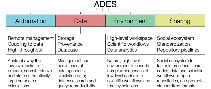
Figure 1: The four pillars of the proposed infrastructure for computational science. At the lower level, an automation framework and an efficient data management solution are needed. At the user level, a high-level environment is coupled with a social ecosystem to stimulate the sharing of codes, data and workflows.

The first pillar, Automation, responds to the needs of abstracting away the low-level tasks to prepare, submit, retrieve and store large numbers of calculations. It can be subdivided into the following main items:

• Remote management Large computations are typically prepared on a user’s workstation and executed on HPC clusters. The different steps of job preparation, submission, status check, and results retrieval are repetitive and independent of the specific simulation tool. Therefore, remote management tasks can be abstracted into an Application Programming Interface (API) and automated. Different communication and scheduler implementations can be supported by plugins, all adopting the same API, as we discuss in Sec. 4.2.

• Coupling to data Full reproducibility of calculations requires a tight coupling of automation and storage. Decoupling these two aspects leaves the researcher with the error-prone task of manually uploading calculation inputs and outputs to a suitable repository, with the additional risk of providing incomplete information. Instead, if the repository is populated first by the user with all the information needed to run the simulation, the process of creating the input files and running the calculation can be automated and easily repeated. The resulting repositories are therefore necessarily consistent; moreover, almost no user intervention is required to create direct pipelines to shared repositories, as the data is already stored coherently.

• High-throughput The main advantage of automation is obtained in situations when screening or parameter sweeps are required, involving thousands of calculations or more. Running and managing them one by one is not feasible. Having a high-level automation framework opens the possibility to run multiple calculations simultaneously, analyze and filter the results. The infrastructure must be able to deal with potential errors arising during the computations, trying to automatically recognize and remedy these whenever possible.

The second pillar, Data, concerns the management of the data produced by the simulations and covers the following three core areas:

• Storage HPC calculations produce a large amount of heterogeneous data. Files containing input parameters and final results need to be automatically and permanently stored for future reference and analysis. On the other hand, much of the data is required only temporarily (e.g., for check-pointing) and can be discarded at the end of the simulation. Therefore, a code-dependent file-storage policy (optionally customizable by the user) must be adopted to categorize each output file. Anyhow, the existence of intermediate files should be recorded, so that the logical flow of calculations is persisted even when restart files are deleted. If the platform ensures reproducibility of calculations, it is straightforward to regenerate the intermediate files, if needed. It is also important to store information on the codes that generated the data. If ultimate reproducibility is needed, one could envision to store reference virtual machines or Docker [17] images with the code executables.

• Provenance To achieve reproducibility, the platform needs to store and represent the calculations that are executed, together with their input data. An effective data model, though, should not only put emphasis on calculations and data, but also keep track of the causal relationships between them, i.e., the full provenance of the results. For instance, a final relaxed crystal structure is of limited use without knowing how it was obtained. The natural data structure to represent the network of relations between data and calculations is a directed acyclic graph, as we will motivate in greater detail in Sec. 4.1.

• Database Today’s typical computational work environment consists of a multitude of files with arbitrary directory structures, naming schemes and lacking documentation. In practice, it is hard to understand and use the information (even by the author after some time) and to retrieve a specific calculation when many are stored. A database can help in organizing results and querying them. The implementation of the data model discussed above, based on directed acyclic graphs, must not be restricted to a specific application, but has to accommodate heterogeneous data. It must be possible to efficiently query any attribute (number, string, list, dictionary, …) associated to a graph node. Queries that traverse the graph to assess causal relationships between nodes must also be possible. A graph database backend is not required if the requirements above are satisfied. For instance, AiiDA’s backend is a relational database with a transitive-closure table for efficient graph-traversal (see Secs. 5.2 and 5.3).

The first two pillars described above address mainly low-level functionalities. The next two pillars deal instead with user-oriented features. In particular, the pillar Environment focuses on creating a natural environment for computational science, and involves the following aspects:

• High-level workspace As the researcher’s objective is to make new discoveries and not to learn a new code, the infrastructure should be flexible and straightforward to use. For instance, while databases offer many advantages in data-driven computational science, few scientists are expert in their administration. For this reason, the intricacies of database management and connections must be hidden by the an API abstraction layer. Furthermore, by adopting a widespread high-level programming language (such as Python) one can benefit of mature tools for inserting and retrieving data from databases [18, 19, 20]. The infrastructure must also be modular: a core providing common low-level functionalities, and customizable plugins to support different codes.

• Scientific workflows Much of the scientific knowledge does not merely lie in the final data, but in the description of the process, i.e., the “scientific workflow” used to obtain them. If these processes can be encoded, then they can be reused to compute similar quantities in different contexts. A workflow specifies a dependency tree between calculation steps, that may not be defined at the start, but depend on intermediate results (e.g., an iterative convergence with an unpredictable number of iterations). Therefore, the infrastructure should automatically generate dependent calculations only when their inputs are available from earlier steps, evaluating dependencies at run-time. The integration of the scientific workflows with the other infrastructure pillars helps the users to focus on the workflow logic rather than on the details of the remote management. As an additional benefit, the automatic storage of the provenance during execution provides an implicit documentation of the logic behind the results.

• Data analytics Application-driven research has the necessity of using dozens of different tools and approximations. Nevertheless, results obtained with different codes often require the same post-processing or visualization algorithms. These data types (e.g., crystal structures or band structures) should be stored in the same common format. The infrastructure can then either provide data analytics capabilities to perform operations on them, or even better facilitate the adoption of existing libraries. This result can be achieved by providing interfaces to external tools for data processing and analytics (e.g. [21, 22] for crystal structures), regardless of the specific simulation code used to generate the data.

The fourth pillar, Sharing, envisions the creation of a social ecosystem to foster interaction between scientists, in particular for sharing data, results and scientific workflows:

• Social ecosystem The envisioned framework should be an enabling technology to create a social ecosystem in computational research. Data access policies must be considered with great care. Researchers prefer at times to keep their data private (while protecting information in pending patents or unpublished data), but sharing with collaborators or on a public repository should occur with minimal effort, when desired. Beside data sharing, a standardized plugin interface should be provided. Plugin repositories can be set up, to which users can contribute to share workflows, handlers for new data formats, or support for new simulations codes. By this mechanism, scientists will be able to engage in social computing, parallel to the developments in the mobile app and web ecosystems.

• Standardization In order to facilitate data exchange, standard formats should be agreed upon and adopted for data sharing (e.g. [23]). Even when multiple standards exist, a hub-and-spoke configuration can be envisaged, where each new code has the task to provide the data in an established format. On the other hand, it is important that suitable ontologies are defined (i.e., simplifying, the names and physical units of the quantities to store in a given repository, together with their meaning). Ontologies are field-specific and their definition must be community-driven (an example of an ongoing effort is the TCOD [24] database). The infrastructure can be useful in this respect both as an inspiration for the ontology, and as a testing environment containing a set of simulated use cases.

• Repository pipelines As more repositories emerge, it is important to develop the ability to import or export data directly, either through REST interfaces or via suitably defined protocols. If formats and ontologies are established, the platform must simply convert the data and its provenance in the specified format. Contributing to external databases becomes straightforward and the platform becomes a facilitator for the creation of shared repositories.

3 The AiiDA infrastructure

The ADES model described in the previous section aims at defining an integrated infrastructure for automating, storing, managing and sharing simulations and their results. Until now, we discussed the model at an abstract level, so as to highlight the generality of the requirements. In order to provide researchers with an effective tool to manage their efforts, we developed a Python infrastructure (“AiiDA”, http://www.aiida.net) that is distributed open-source. In the following, we describe the implementation details of AiiDA, with particular emphasis on how the requirements of Sec. 2 have been met.

We start by outlining the architecture of AiiDA, schematically represented in Fig. 2. AiiDA has been designed as an intermediate layer between the user and the HPC resources, where automation is achieved by abstraction.

The core of the code is represented by the AiiDA API, a set of Python classes that expose to the user an intuitive interface to interact with the main AiiDA objects — calculations, codes and data — hiding the inhomogeneities of different supercomputers or data storage solutions. The key component of the API is the Object–Relational Mapper (ORM), a layer that maps AiiDA storage objects into python classes. Using the ORM, these objects can be created, modified and queried via a high-level interface which is agnostic of the detailed storage solution or of the SQL query language. The details of the storage, composed of both a relational database and a file repository, are discussed in Sec. 5.

The user interacts with AiiDA in different ways: using the command line tool verdi, via the interactive python shell, or directly through python scripts (more details in Sec. 6.3). Most components are designed with a plugin architecture (Sec. 6.2). Examples of features that can be extended with new plugins include the support of new simulation codes, management of new data types, and connection to remote computers using different job schedulers.

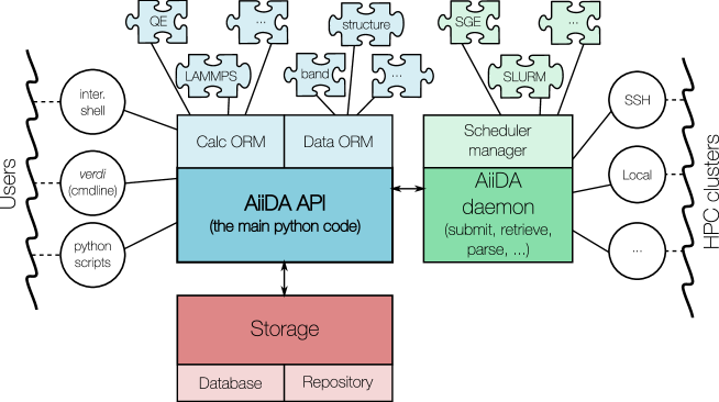
Figure 2: The main components of the AiiDA infrastructure and their interactions. The core AiiDA component is the API, whose ORM represents stored objects as python classes. AiiDA supports any computational code and data type via a plugin interface. The AiiDA daemon is a background process that takes care of most automated operations such as job submission, scheduler state check, file retrieval and parsing. It interacts with the remote clusters via different channels (local, ssh, …) using the appropriate scheduler plugins.

4 Automation in AiiDA

4.1 The AiiDA daemon

The daemon is one important building block of AiiDA: it is a process that runs in the background and handles the interaction with HPC clusters (selecting the appropriate plugins for the communication channels — like SSH — or for the different job schedulers, see Sec. 4.2 below) and takes care of all automation tasks. Once the daemon is started, it runs in the background, so that users can even log out from their accounts without stopping AiiDA. Internally, it uses celery [25] and supervisor [26] to manage asynchronous tasks.

The fundamental role of the daemon is to manage the life cycle of single calculations. The management operations are implemented in the aiida.execmanager module and consists in three main tasks: 1) submission of a new job to a remote computer, 2) verification of the remote job scheduler state, and 3) retrieval and parsing of the results after a job completion. These steps are run independently. If several calculations are running on the same machine, they are grouped in order to open only one remote connection and avoid to overload the remote cluster.

The user can follow the evolution of a calculation without connecting directly to the remote machine by checking the state of a calculation, an attribute that is stored in the database and is constantly updated by the daemon. In particular, every calculation is initialized in a NEW state. A call to the calc.submit() method brings calc to the TOSUBMIT state. As soon as the daemon discovers a new calculation with this state, it performs all the necessary operations to submit the calculation and then sets the state to WITHSCHEDULER. Periodically, the daemon checks the remote scheduler state of WITHSCHEDULER calculations and, at job completion, the relevant files are automatically retrieved, parsed and saved in the AiiDA storage. Finally, the state of the calculation is set to FINISHED, or FAILED if the parser detects that the calculation did not complete correctly. Beside the aforementioned states, other transition states exist (SUBMITTING, RETRIEVING, PARSING) as well as states to identify failures occurred in specific states (SUBMISSIONFAILED, RETRIEVALFAILED and PARSINGFAILED).

4.2 Transports and schedulers

As discussed in the “Remote management” section of the “Automation” pillar, in AiiDA we define an abstract API layer with methods to connect and communicate with remote computers and to interact with the schedulers. Thanks to this API, the internal AiiDA code and the user interface are independent of the type of connection protocol and scheduler that are actually used.

The generic job attributes valid for any scheduler (wall clock time, maximum required memory, name of the output files, …) are stored in a common format. For what concerns schedulers, early work in the specification of a middleware API has been done in the Open Grid Forum [27] with, e.g., the DRMAA [28] and the SAGA APIs, and similar efforts have been done by the UNICORE [29] and gc3pie [30] projects. In AiiDA, we have taken inspiration from these efforts. We provide appropriate plugins to convert the abstract information to the specific headers to be written at the top of the scheduler submission file. Moreover, the plugins provide methods that specify how to submit a new job or how to retrieve the job state (running, queued, …). Plugins for the most common job schedulers (Torque [31], PBS Professional [32], SLURM [33], SGE or its forks [34]) are already provided with AiiDA.

The scheduler plugins and the daemon, then, rely on the transport component to perform the necessary remote operations (file copy and transfer, command execution, …). Also in this case, we have defined an abstract API specifying the standard commands that should be available on any transport channel (connection open and close, file upload and download, file list, command execution, …). Plugins define the specific implementation. With AiiDA, we provide a local transport plugin, to be used if AiiDA is installed on the same cluster on which calculations will be executed. This plugin performs directly command execution and file copy using the os and shutil Python modules. We also provide a ssh transport plugin to connect to remote machines using an encrypted and authenticated SSH channel, and SFTP for file transfer. In this case, AiiDA relies on paramiko [35] for the Python implementation of the SSH and SFTP protocols.

The appropriate plugins to be used for each of the configured computers are specified only once, when user configures for the first time a new remote computer in AiiDA.

5 Data in AiiDA: database, storage and provenance

5.1 The data model in AiiDA

The core concept of the AiiDA data model, partially inspired by the Open Provenance Model [36], is that any calculation acts as a function (with the meaning this word has in mathematics or in a computer language), performing some manipulation on a set of input data to produce new data as output.

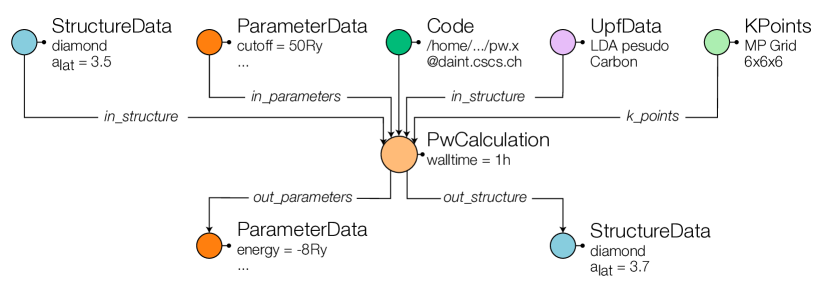
Figure 3: A simple example of how a calculation, the executable code and input/output data are represented as nodes in a graph. Labeled links between nodes represent logical relationships: either inputs or outputs. The code in input of a calculation represents the executable that is launched. In this example, a Quantum ESPRESSO code is used to relax a diamond crystal, using further parameters as input nodes (cutoffs, a mesh of $k-$points, a pseudopotential in UPF format for carbon, …). In output, two nodes are produced: a list of result parameters (e.g., the total energy) and an output relaxed structure. This node can in turn be used as input of new calculations.

We thus represent each fundamental object, Calculation and Data, as a node in a graph. These nodes can be connected together with directional and labeled links to represent input and output data of a calculation. Direct links between Data nodes are not allowed: any operation (even a simple copy) converting data objects to other data objects is a function and must thus be represented by an intermediate Calculation node. We define for convenience a third fundamental object, the Code, representing the executable file that is run on the HPC resource. Each Calculation has therefore a set of Data nodes and a Code node as input (Fig. 3). As the output Data nodes can in turn be used as input of new calculations, we are effectively modeling a Directed Acyclic Graph (DAG) representing the chain of relationships between the initial data (e.g., a crystal structure from an experimental database) and the final results (e.g., a luminescence spectrum) through all the intermediate steps that are required to obtain the final result: the provenance information of the data is therefore saved. (The graph is acyclic because links represent a causal connection, and therefore a loop is not allowed.)

5.2 The AiiDA database

Given that AiiDA represents data in terms of DAGs, we need to choose an efficient way to save them on disk. The objects we need to store are the nodes and the links between them. Each node needs to contain all the information describing it, such as lists of input flags, sets of parameters, list of coordinates, possibly some files, etc. Therefore, the actual implementation must support the storage of arbitrary lists of files, and of attributes in the form key=value (of different types: strings, numbers, lists, …) associated to each node. One simple solution could consist in storing one file per node, containing all node attributes in a suitable format, and then store all the links in another file. However, this storage type is clearly not efficient for querying, because in the absence of a suitable indexing system every search requires disk access to each file. A database, instead, can speed up queries significantly. To have a net benefit however, the database must be suitably configured for the specific type of data and queries that are most likely expected. Moreover, different database solutions exist, each of them tailored to specific types of data.

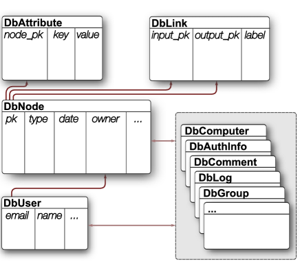
Figure 4: The most relevant tables of the AiiDA database schema. The DbNode table contains an entry for each node, with only a limited set of columns such as the ID (or primary key, PK), a string identifying the type of node (Calculation, Data, Code, or a subclass), the creation date, and the owner (a foreign key to the DbUser table). All other attributes are stored in the DbAttribute table, as described in the text. A third DbLink table stores all the links (each link being identified by the PK of the input and output endpoints, and by a label). Other tables exist in the database (to store computers, authorization information, comments, log messages, groups, …) typically referencing both to nodes and users (e.g., the comment of a given user on a given node).

In this section, we discuss only the details of the storage solution implemented in AiiDA, and we defer to A.1 a discussion on database types (e.g. SQL vs. NoSQL) and on the reasons for our implementation choices. After benchmarking different solutions, we have chosen to adopt a SQL backend for the AiiDA database. In particular, MySQL [37] and PostgreSQL [38] are fully supported, together with the file-based backend SQLite [39] (even if the latter is not suited for multiple concurrent accesses, and its usage is limited to testing purposes). The database is complemented by a file repository, where arbitrary files and directories can be stored, useful for large amounts of data that do not require direct querying, and is going to be discussed in details later in Sec. 5.4. In our implementation, the three main pieces of information of the DAG (nodes, links, and attributes) are stored in three SQL tables, as shown in Fig. 4.

The main table is called DbNode, where each entry represents a node in the database. Only a few static columns are defined: an integer identifier (ID), that is also the Primary Key (PK) of the table; a universally-unique identifier or UUID, a “type” string to identify the type of node (Calculation, Data, Code, or one of their subclasses, see Sec. 6.1). A few more columns exist for “universal” information such as a label, the creation and modification time, and the user who owns the node (a foreign link to the DbUser table, storing user details).

A second table, DbLink, keeps track of all directional links between nodes. Each entry contains the PKs of the input and output nodes of the link, and a text field for the link label, that distinguishes the different inputs to a calculation node (e.g., a crystal structure, a set of parameters, a list of k-points, etc.). For instance, link names used for a Quantum ESPRESSO calculation can be seen in Fig. 3.

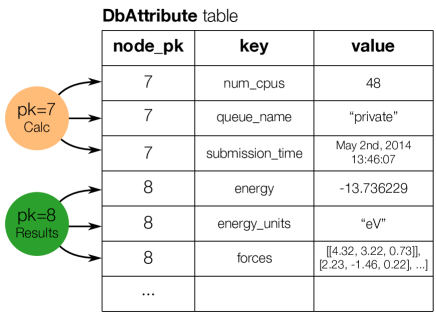
Figure 5: Arbitrary attribute data in a SQL EAV table by means of our DbAttribute table. This schema is simplified; the actual schema implemented in AiiDA is described in A.1.

A third table, DbAttribute, is used to store any possible attribute that further characterizes each node. Some examples of attributes could be: an energy value, a string for the chemical symbol of each atom in a crystal structure, a $3\times 3$ matrix for the components of the crystal vectors, an integer specifying the number of CPUs that we want to use for a given calculation, …

The DbAttribute table is schematically represented in Fig. 5. Each entry represents one attribute of a node, and for each attribute we store: the PK of the node to which this attribute belongs; the key, i.e. a string defining the name of the property that we want to store (e.g. “energy”, “atom_symbols”, “lattice_vectors”, “num_cpus”, …); and the value of the given property. Internally, the table has a more complicated schema allowing for extended flexibility:

• Different primitive data types can be stored (booleans, integers, real values, strings, dates and times, …)

• Arbitrary Python dictionaries (sets of key=value pairs) and lists can be stored, and any element of the list or of the dictionary can be directly and efficiently queried (even in case of multiple depth levels: lists of lists, lists of dictionaries, …)

The technical description of the EAV table is deferred to A.1. We emphasize here that by means of this table we achieve both flexibility, by being able to store many data types as an attribute, and preserving query efficiency, since any element in the database can be queried directly at the database level (making full use of indexes, etc.).

Since each row of the DbAttribute table is an internal property of a single node, we enforce that attributes cannot be modified after the respective node has been permanently stored (for example, we do not want the number of CPUs of a calculation to be changed after the calculation has been stored and executed). However, the user will often find it useful to store custom attributes for later search and filtering (e.g., a tag specifying the type of calculation, the spacegroup of a crystal structure, …). To this aim, we provide a second table (DbExtra) that is identical to the DbAttribute table (and therefore it has the same data storage and querying capabilities). The content of the DbExtra table, though, is not used internally by AiiDA, and is at complete disposal of the user.

Besides the three tables DbNode, DbLink and DbAttribute that constitute the backbone of the database structure, there are a few other tables that help data management and organization. The most relevant are:

• DbUser contains user information (name, email, institution).

• DbGroup defines groups of nodes to organize and gather together calculations belonging to the same project, pseudopotentials of the same type, etc.

• DbComputer stores the list of remote computational resources that can be used to run the simulations.

• DbAuthInfo stores the authorization information for a given AiiDA user (from the DbUser table) to log in a given computer (from the DbComputer table), like the username on the remote computer, etc.

• DbWorkflow, DbWorkflowData, DbWorkflowStep are the tables that store workflow-related information.

• DbPath is the transitive closure table, described in the next section.

5.3 Graph database: querying the provenance

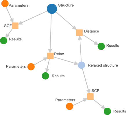
Figure 6: A schematic example of a possible graph inside the AiiDA database. An initial crystal structure (blue node on the top of the figure) is used both for a total energy calculation (SCF) and for a structural relaxation calculation (Relax). Each calculation has a set of input parameters (orange dots) and of output results (dark green dots). The relaxation calculation also produces another crystal structure, used as input for a new SCF calculation. Moreover, the two structures in the graph are both taken as input from a calculation that computes a suitably-defined “distance” between them.

An example of a simple graph that can be stored in AiiDA is shown in Fig. 6, where four different calculations have been run with different inputs producing a set of output results, and where some output nodes have been used as input of new calculations. Using the database data model described in the previous section, we can store DAGs with arbitrary queryable attributes associated to each node. However, there is another type of query specific to graph databases, related to the graph connectivity: given two nodes, to determine the existence of a path connecting them. This is particularly relevant for simulations in Materials Science: typical queries involve searching for crystal structures with specific computed properties, but the number of intermediate steps (i.e., Calculation nodes) between a structure data node and the final result can be large and not even predictable (e.g., if multiple restarts are required, …). This type of searches requires in practice to query the provenance of the data in the database.

Sophisticated and efficient graph traversal techniques have been developed to discover the existence of a path between two nodes, and graph databases (e.g., Neo4j [40]) implement these functions at the database level, however they require the use of custom querying languages. Instead, we address the graph traversal problem within a SQL database by incrementally evaluating a transitive closure table (that we called DbPath). This table lists the “paths”, i.e., all pair of nodes (“parent” and “child”) that are connected together in the graph through a chain of links. The table is automatically updated every time a link is added, updated or removed from the DbLink table, by means of database triggers that we have developed for the three supported backends (SQLite, MySQL and PostgreSQL). The algorithm for the update of the transitive closure table has been inspired by Ref. [41] and is described in detail in A.2.

Obviously, the DbPath table allows for fast queries on the data “history”, at the expense of occupying additional disk space for its storage. The size of the table can in general become very large; however, in Material Science applications, we typically do not have a single dense graph where all nodes are interconnected; instead, one often creates many small graphs of the type of Fig. 6. This means that the size of the DbPath table will remain roughly linear in the number of nodes in the graph. After benchmarking, we have chosen the solution described above as a good compromise between storage and query efficiency.

5.4 Database vs. file repository

The storage of attributes in the database discussed previously allows for query efficiency, at the price of disk space (for additional information like indexes, data types, …) and of efficiency in regular operations (retrieving a large list from the database is slower than retrieving a file containing the same list). For large matrices, therefore, a threshold exists above which the advantages of faster query speed are not justified anymore. Moreover, the single entries of a large matrix (like the electron charge density discretised on a grid) are often of little interest for direct querying. In such cases it is convenient to store data in a file and rely on the file system for I/O access. This is especially appropriate when the data should be used as an input to another calculation and a fast read access is required.

For these reasons, AiiDA complements the database storage with a file repository (see Fig. 2), confined within a folder configured during the setup phase of AiiDA. Every time a new node is created, AiiDA automatically creates a subfolder for the specific node. Any file, if present, associated with the node will be stored therein.

Storing information as files or in the database is left as a choice for the developers of the specific subclass of the Data of Calculation nodes (plugins are discussed in Sec. 6.1), but in order to maximize efficiency, it should follow the guideline discussed above. Some examples of the choices made for some AiiDA Data plugins can be found in Sec. 6.2.

6 The scientific environment in AiiDA

6.1 The ORM

AiiDA is written in Python, a powerful object-oriented language. The materials simulation community has been moving towards Python in recent years, due to its simplicity and the large availability of libraries for visualization, text parsing, and scientific data processing [10, 21, 42]. An important component of the AiiDA API is the Object-Relational Mapper (ORM), which exposes to the user only a very intuitive Python interface to manage the database. The main class of the AiiDA ORM, Node, is used to represent any node in the graph. Each instance of the Node class internally uses Django to perform database operations, and complements it with methods for accessing the file repository. The low-level interaction with the database uses the Django framework [18].

The main functionalities of the Node class are:

• It provides a direct access to the node attributes, accessible as a Python dictionary by using the node.attrs() method. The method also properly recreates lists and dictionaries that were stored in expanded format at the database level (lists and dictionaries are not natively supported in the chosen databases), as described in A.1. Similar methods allow the user to read and write user-defined attributes in the DbExtra table.

• It provides direct access to the repository folder containing the files associated to each Node.

• It provides a caching mechanism that allows the user to create and use the Node even before storing it in the database or on the repository folder, by keeping the files in a temporary sandbox folder, and the attributes in memory. This is particularly useful to test the generation of the input files by AiiDA without the need to store test data in the database. Only after the node.store() call, all the data is permanently stored in the AiiDA database and repository and no further modifications are allowed. A similar caching mechanism has also been implemented to keep track of links between nodes before storing.

• It provides an interface for querying nodes with specific attributes or with specific attribute values, or nodes with given inputs or outputs, etc.

• It provides methods (.inp and .out) to get the list of inputs and outputs of a node and similarly the list of all parent and child nodes using the transitive closure table.

6.2 The plugin interface

To support a new type of calculation or a new kind of data (e.g. a band structure, a charge density, a set of files, a list of parameters, …), one simply needs to write an AiiDA plugin. A plugin is simply a python module file, containing the definition of a subclass of the AiiDA classes, sitting in an appropriate folder; AiiDA automatically detects the new module and uses it.

All different types of nodes are implemented as subclasses of the Node class. At a first subclass level we have the three main node types: Calculation, Code and Data. Each of them is further subclassed by plugins to provide specific functionalities. In particular, instances of Code represent a specific executable file installed on a given machine (in the current implementation, there are no further subclasses). Each subclass of Calculation, instead, supports a new simulation software and contains the code needed to generate the software-specific input files starting from the information stored in the AiiDA database. Moreover, it can also provide a set of software-dependent methods (like calc.restart(), …) that make it easier for the user to perform routine operations. Finally, the Data class has a subclass for each different type of data that the user wants to represent. The specific subclass implementation determines the possible user operations on the data, and whether the information is going to be stored in the database as attributes or in the file repository. We report here a description of some of the most relevant Data subclasses distributed with AiiDA:

• ArrayData: it is used to store (large) arrays. Each array is stored on disk as a binary, portable, compressed file using the Python numpy module [43]. Some attributes are stored in the DbAttribute table for fast querying (like the array name and its size). Subclasses use the same storage model, but define specific methods to create and read the data (e.g., the KpointsData class has methods to detect a structure cell, build the list of special $k$-points in $k$ space and create paths of $k$-points, suitable for plotting band structures, using for instance the standard paths listed in Ref. [44]).

• ParameterData: it is used to store the content of a Python dictionary in the database. Each key/value pair is stored as an attribute in the DbAttribute table, and no files are stored in the repository.

• RemoteData: this node represents a “link” to a directory on a remote computer. It is used for instance to save a reference to the scratch folder on the remote computer in which the calculation was run, and acts as a placeholder in the database to keep the full data provenance, for instance if a calculation is restarted using the content of that remote folder. No files are written in the AiiDA repository, but the remote directory absolute path is stored as an attribute.

• FolderData: this node represents a folder with files. At variance with RemoteData, files are stored permanently in the AiiDA repository (e.g., the outputs of a finished calculation retrieved from the remote computer).

• StructureData: this node represents a crystal structure. The $3\times 3$ coordinates of the lattice vectors, the list of atoms and their coordinates, and any other information (atomic masses, …) are saved as attributes for easy querying. (For very large structures, a different data model may be more efficient.) Methods are provided for standard operations like getting the list of atoms, setting their positions and masses, converting structures to and from other formats (e.g. the Atoms class of the ASE Atomistic Simulation Environment [21]), obtaining the structure from an external database (like ICSD [45] or COD [46]), getting the spacegroup using SPGlib [42], etc.

Finally, we emphasize that the plugin interface is not limited to the ORM, and a similar plugin-based approach applies to other AiiDA components, like the connection transport channel and the schedulers (as discussed in Sec. 4.2).

6.3 User interaction with AiiDA

We provide a few different interfaces to interact with AiiDA. The most commonly used is the verdi command line utility. This executable exposes on the command line a set of very common operations, such as performing the first installation; reconfiguring AiiDA; listing or creating codes, computers and calculations; killing a calculation; starting/stopping the daemon, … The verdi tool is complemented by a Bash completion feature to provide suggestions on valid commands by pressing the TAB key. Moreover, an inline help provides a list of existing commands and a brief description for each of them. The advantage of verdi is to expose basic operations to the user without requiring any knowledge of Python or other languages.

In order to access the full AiiDA API, however, the best approach is to write Python scripts. The only difference with respect to standard python scripts is that a special function aiida.load_dbenv() needs to be called at the beginning of the file to instructs Python to properly load the database. Once this call has been made, any class from the aiida package can be loaded and used. If the users do not want do explicitly call the aiida.load_dbenv() call in the python code, then they can run the script using the verdi run command. In this case, the AiiDA environment and some default AiiDA classes are automatically loaded before executing the script.

A third interface is the interactive python shell that can be loaded using the command verdi shell. The shell is based on IPython [47] and has the advantage to automatically load the database environment; at the same time, it already imports by default some of the most useful classes (e.g. Node, Calculation, Data, Group, Computer, …) so that they are directly available to the user. TAB completion is available and very useful to discover methods and attributes. Moreover, the documentation of each class or method (written as Python “docstrings”) is directly accessible.

6.4 Scientific workflows

As introduced in Sec. 2, many tasks in scientific research are standard and frequently repeated, and typically require multiple steps to be run in sequence. Common use cases are parameter convergence, restarts in molecular dynamics simulations, multi-scale simulations, data-mining analysis, and other situations when results of calculations with one code are used as inputs for different codes. In such cases, it is beneficial to have a system that encodes the workflow and manages its execution [48, 49, 50, 51, 52].

In order to fully integrate the workflows within the ADES model, we implement a custom engine into AiiDA, by which the user can interact with all AiiDA components via the API. This engine is generic and can be used to define any computational workflow. Specific automation schemes, crafted for selected applications (equation of states, phonons, etc…) are implemented within each workflow and can be developed directly by the users.

AiiDA workflows are subdivided into a number of steps. One or more calculations can be associated to each step; these are considered to be independent and are launched in parallel. Instead, different steps are executed sequentially and the execution order is specified by “forward” dependency relationships: In other words, each “parent” step must specify the step to be executed next. The execution of the “child” step is delayed until all calculations associated to the parent have completed. We emphasize that dependency relationships are defined only between steps. Dependencies between calculations are implicit, with the advantage of allowing for both parallel and serial simulation streams.

Within a step, beside creating calculations and associating them to the current step, any other Python (and AiiDA) command can be executed. This gives maximum flexibility to define complex workflow logics, especially if the outputs of a calculation in a parent step require some processing to be converted to the new calculation inputs. Moreover, a step can define itself as the next step to be executed, providing support for loops (even conditional ones, where the number of iterations depends on the calculations results).

A key feature, modularity, completes AiiDA workflows: within each step, the user can associate not only calculations, but also subworkflows. The advantage is the possibility to reuse existing workflows that perform specific tasks, so as to develop only missing features. For instance, let us assume that we developed a workflow “A” that performs a DFT calculation implementing code-specific restart and recover routines in order to make sure convergence is achieved. Then, a workflow “B” that calculates the energy of a crystal at different volumes (to obtain its equation of state) does not need to reimplement the same logic, but will just reuse “A” as a subworkflow. “B” can in turn become a subworkflow of a higher-level workflow “C” that, for instance, compares the equation of state calculated at different levels of approximation. The combination of parallel and serial execution, conditional loops, and modularity, makes the workflows general enough to support any algorithm.

From the implementation point of view, the AiiDA workflow engine is provided by a generic Workflow class, that can be inherited to define a specific workflow implementation. Workflow steps are special class methods identified by the @step decorator. The base class also provides dedicated methods to associate calculations and workflows to the current step. In every step, a call to the self.next() method is used to define dependencies between steps. This method accepts as a parameter the name of the following step. The name is stored in the database, and the corresponding method is executed by the daemon only when all calculations and subworkflows of the current step have finished.

In analogy with calculations, AiiDA uses states to keep track of workflows and workflow steps (RUNNING, FINISHED, …). The AiiDA daemon handles all the workflow operations (submission of each calculation, step advancement, script loading, error reporting, …) and the transitions between different workflow states.

In the long term, we envision integrating into AiiDA many new and existing methods in the form of workflows (e.g., training interatomic potentials [53], crystal structure prediction algorithms [54, 55], …), so that the researcher can focus on materials science and delegate to AiiDA the management of remote computers, the appropriate choice of code-specific parameters, and dealing with code-specific errors or restarts.

6.5 Querying

A relevant aspect of a high-level scientific environment is the possibility of running queries on the data stored in AiiDA without the need to know a specific (and typically complex) query language. To this aim, we have developed a Python class, called the QueryTool, to specify in a high-level format the query to run. For instance, it is possible to specify a filter on the node type (e.g., to get only crystal structures); to filter by the value of a specific attribute or DbExtra table entry (e.g., to select structures with a specific spacegroup); or to filter by a specific attribute in one of the linked nodes (e.g., to get structures on which a total-energy calculation was run, and the energy was lower than a given threshold). Queries can also take advantage of the transitive closure table, setting filters on attributes of nodes connected to the one of interest by an unknown number of intermediate links (e.g., if the result of the calculation was obtained after an unknown number of restarts). As an example, a complex query that can be run with AiiDA is: give me all crystal structures containing iron and oxygen and with a cell volume larger than $X$ Å³, that I used as input for a sequence of calculations with codes $Y$ and $Z$ to obtain the phonon band structure, for which the lowest phonon frequency that was obtained is positive, and for which the DFT exchange-correlation functional used was LDA. Other complex queries can be specified using the QueryTool in a format that is easy both to write and to read.

6.6 Documentation and unit testing

A key component of a productive scientific environment is a complete and accurate code documentation. For this reason, AiiDA is complemented by an extensive documentation. Each class, method and function has a Python docstring that describes what the function does, the arguments, the return values and the exceptions raised. These docstrings are accessible via the interactive shell, but are also compiled using the Sphinx [56] documentation engine into a comprehensive set of HTML pages (see Fig. 7). These pages are distributed with the code (in the docs/ subfolder) and also available online at http://aiida-core.readthedocs.org. Moreover, we also provide in the same format, using Sphinx, a complete user documentation of the different functionalities, supported databases, classes and codes, together with tutorials covering the installation phase, the launch of calculations and workflows, data analysis, … The user guide is also complemented by a developer’s guide that documents the API and contains tutorials for the development of new plugins.

Moreover, to simplify the code maintenance, we implement a comprehensive set of unit tests (using the Python unittest module), covering the different components of AiiDA described in Fig. 2.

Figure 7: The first page of the AiiDA documentation. Different sections are aimed at the end users (with examples and tutorials) and at developers (with the documentation of classes and methods, and tutorials for new plugin development).

7 Sharing in AiiDA

The fourth pillar introduced in Sec. 2 aims at enabling a social ecosystem where it becomes easy to share tools and results, such as data, codes, and workflows. In order to preserve the authorship and privacy of the data of each researcher, we implemented a model in which each user or group of users can install their own local AiiDA instance. All data and calculations are accessible only to people with direct access to the instance and therefore remain private. In order to enable sharing of the database (or parts of it) with collaborators, we provide functionality to export a portion of the database to a file, and then to import it in a different instance of AiiDA. In this way several groups in a collaboration may contribute to a common repository, open to the entire project, while retaining their private portions as needed. This approach simplifies issues of user- and group-level security. To avoid conflicts during this procedure, AiiDA assigns a Universally Unique IDentifier (UUID) to each node as soon as it is locally created. In fact, while for internal database usage an auto-incrementing integer PK is the most efficient solution to refer to a database row, the PK is not preserved when a node is transferred to a different database. Instead, the first node to be created will always have PK=1, the second PK=2, and so on. A UUID is instead a hexadecimal string that may look like the following: e3d21365-7c55-4658-a5ae-6122b40ad04d. The specifications for creating a UUID are defined in RFC 4122 by IETF [57], and they guarantee that the probability that two different UUIDs generated in different space and time locations can be assumed to be zero. In this way, we can use the UUID to identify the existence of a node in the DB; at import time, it is only verified whether a node with the same UUID already exists before including its contents in the database. We envision one or several centralized repositories, available to the public, that collect results from different groups. Researchers will be able to share results with colleagues by exchanging just the UUID of the nodes stored on the public repository, rather than sending actual scripts or files. In this collaborative environment the adoption of new codes, the comparison of results, and data disclosure and reproducibility become straightforward, realizing the “social ecosystem” discussed in Sec. 2 and facilitating the reusability of data, codes and workflows. We emphasize that only after having a locally deployed automation infrastructure like AiiDA it becomes feasible to populate public repositories efficiently and in a uniform format, because the user effort to uniform the data, prepare it and upload it is reduced to the minimum.

The standardization of the formats produced by different codes is necessary to maximize the effectiveness of data sharing. This task is outside the scope of the AiiDA project, but we encourage existing and future standardization efforts by the developers of the simulation codes. At the same time, within AiiDA we provide a set of “default” plugins for the most common data structures (crystal structures, paths of $k-$points in reciprocal space, …), which can be seamlessly reused in different codes. Implemented classes provide importers and exporters from/to common file formats, so that it is possible to exchange the data also with other infrastructures and repositories that use different data formats. We also emphasize that it is possible to write workflows that perform high-level tasks common to a variety of codes, such as structure optimization or molecular dynamics, even before a standardization of data formats takes place.

Moreover, to encourage the development of the repository pipelines discussed in the “Sharing” pillar, we define in AiiDA a common API for importers and exporters of crystal structures (in the aiida.tools package). Also in this case, repositories can be supported by plugin subclasses; plugins for importing structures from some common databases, such as ICSD [45], COD [46], MPOD [58] and TCOD [24] are already distributed with the code.

8 Codes and data types supported out of the box

In the first stage of the development of AiiDA, we mainly focused on the infrastructure and its components (scheduler management, database, …) rather than writing a large number of plugins.

However, we already provide with AiiDA fully-functional plugins for most codes of the Quantum ESPRESSO package [59], namely pw.x, ph.x, cp.x, and many of the post-processing tools such as matdyn.x, q2r.x, …These plugins expose the full functionality of the respective codes, and moreover include not only the input generation routines, but also output parsers. The type and format of the input nodes required by Quantum ESPRESSO is shown in Fig. 3 and described in detail in the code documentation. We also provide a PwImmigrant class to import pw.x calculations that were already run before the adoption of AiiDA.

Similarly to calculations, the user can support new custom tailored data types by defining a new data format. However, to facilitate the standardization of the most common data types, we provide with AiiDA a set of Data subclasses. Some examples (already described in Sec. 6.2) include the StructureData for crystal structures (supporting also non-periodic systems, vacancies and alloys), the KpointsData for paths in $k-$space, the BandsData for band-structure data, the ArrayData for generic arrays. Moreover, we also provide a specific class to support pseudopotentials in the UPF format, that is the format used by Quantum ESPRESSO. Specific routines allow the user to upload a single pseudopotential, or a family of pseudopotentials into the database. At upload time, the pseudopotentials are parsed to discover to which element they correspond, and an attribute is added for later querying. Moreover, the MD5 checksum of the file is calculated and stored, to avoid to store twice the same pseudopotential in the database. The verdi data upf uploadfamily command can be used to take all UPF files contained in a folder, possibly of the same type (e.g. ultrasoft with PBE functional, …) and group them in a “family”. In this way, when running a Quantum ESPRESSO simulation, one can ask AiiDA to simply select the appropriate pseudopotentials from a family, rather than manually selecting the pseudopotentials one by one.

We include support also for other codes, in particular all the codtools [60], a set of tools for processing, filtering and correcting CIF files (the de-facto standard format for crystal structures). Furthermore, a basic support to the GPAW code [61] is provided and, since GPAW runs via the ASE interface [21], the same plugin can be used to access a large family of simulation codes already supported by ASE, like VASP, ABINIT, Gaussian, …The full list can be found on the ASE webpage.

9 Examples of applications

In this section, we summarize some examples in the field of materials science in which AiiDA has already been used as the platform for managing simulations.

9.1 Verification and validation

Tests for verification and validation purposes can often be automated. One typical example in the field is the test of pseudopotentials for accuracy and transferability. AiiDA workflows can be developed to perform standardized tests with minimal user intervention, as soon as a new pseudopotential file (or family of pseudopotentials) is available. If a pseudopotential is discovered to be inaccurate, one can easily find and flag all calculations that were performed with it. One can then easily run again all affected calculations with an improved pseudopotential with minimal effort, since each calculation stored in AiiDA is reproducible and the provenance of the data is available.

As an example, we implemented a workflow (using Quantum ESPRESSO as the simulation engine) to perform the Crystalline Monoatomic Solid Test (CMST) with the 15-point protocol described in Ref. [62]. The workflow, starting from an initial guess of the lattice parameter $a_{0}$, iteratively refines the value of $a_{0}$ by fitting a Birch–Murnaghan equation of state to 15 calculations performed at different volumes. An automatic restart procedure is implemented as a subworkflow to automatically relaunch any calculation that crashed using different numerical parameters, as discussed in Sec. 6.4 (e.g. using a different initial guess for the wavefunctions or a different convergence algorithm). We have been able to reproduce the results for the PSlibrary [63] family of pseudopotentials reported in Ref. [62], and we computed the same quantities also for the GBRV pseudopotentials [64] using the suggested cutoffs (40 Ry for the wavefunctions and 200 Ry for the charge density), a shifted $32\times 32\times 32$ $k-$mesh and a Marzari-Vanderbilt smearing [65] of 2 mRy. The results are reported in Table 1.

	FCC			BCC				SC
Element	$a_{0}$	$B_{0}$		$a_{0}$	$B_{0}$	$\Delta E^{fcc}$		$a_{0}$	$B_{0}$	$\Delta E^{fcc}$
Ag	$4.151$	$90.7$		$3.302$	$88.7$	$0.031$		$2.752$	$66.4$	$0.332$
Ba	$6.357$	$8.1$		$5.024$	$8.7$	$-0.017$		$3.955$	$7.8$	$0.287$
Be	$3.163$	$119.8$		$2.506$	$125.2$	$0.018$		$2.176$	$76.5$	$0.920$
Ca	$5.527$	$17.4$		$4.384$	$15.5$	$0.017$		$3.515$	$10.7$	$0.393$
Cd	$4.509$	$41.9$		$3.609$	$36.4$	$0.051$		$3.000$	$30.4$	$0.114$
Co	$3.452$	$257.7$		$2.760$	$242.8$	$0.255$		$2.281$	$186.6$	$0.864$
Cr	$3.625$	$236.6$		$2.850$	$257.4$	$-0.393$		$2.342$	$186.2$	$0.632$
Cs	$7.770$	$2.0$		$6.161$	$2.0$	$0.001$		$5.043$	$1.6$	$0.093$
Cu	$3.633$	$141.7$		$2.888$	$139.7$	$0.035$		$2.409$	$104.1$	$0.469$
Fe	$3.448$	$287.0$		$2.757$	$270.4$	$0.317$		$2.266$	$209.4$	$0.961$
K	$6.664$	$3.6$		$5.282$	$3.6$	$0.000$		$4.295$	$2.9$	$0.105$
Li	$4.325$	$13.8$		$3.435$	$13.9$	$0.002$		$2.732$	$12.2$	$0.121$
Mg	$4.524$	$35.2$		$3.580$	$35.4$	$0.016$		$3.022$	$22.7$	$0.367$
Mn	$3.505$	$279.7$		$2.785$	$278.1$	$0.079$		$2.284$	$211.9$	$0.862$
Mo	$4.000$	$238.0$		$3.160$	$258.8$	$-0.426$		$2.599$	$187.6$	$0.733$
Na	$5.293$	$7.7$		$4.198$	$7.7$	$0.000$		$3.412$	$6.1$	$0.119$
Nb	$4.216$	$164.1$		$3.309$	$172.2$	$-0.324$		$2.719$	$130.0$	$0.664$
Ni	$3.510$	$204.5$		$2.792$	$200.4$	$0.054$		$2.323$	$148.3$	$0.668$
Pd	$3.943$	$170.2$		$3.137$	$167.3$	$0.044$		$2.615$	$123.8$	$0.516$
Rb	$7.147$	$2.8$		$5.667$	$2.8$	$0.001$		$4.622$	$2.2$	$0.095$
Rh	$3.832$	$256.3$		$3.071$	$235.5$	$0.357$		$2.538$	$187.5$	$0.798$
Ru	$3.809$	$307.2$		$3.051$	$281.2$	$0.514$		$2.510$	$221.3$	$1.025$
Sc	$4.618$	$51.3$		$3.676$	$53.4$	$0.056$		$2.967$	$35.2$	$0.721$
Sr	$6.020$	$11.3$		$4.756$	$12.1$	$0.005$		$3.853$	$7.0$	$0.385$
Tc	$3.870$	$298.4$		$3.080$	$293.1$	$0.183$		$2.531$	$223.6$	$0.977$
Ti	$4.113$	$107.6$		$3.255$	$106.0$	$0.053$		$2.640$	$76.7$	$0.780$
V	$3.816$	$176.5$		$2.996$	$183.5$	$-0.244$		$2.448$	$136.8$	$0.607$
Y	$5.060$	$39.4$		$4.039$	$39.0$	$0.098$		$3.262$	$25.8$	$0.773$
Zn	$3.931$	$69.2$		$3.133$	$63.4$	$0.063$		$2.630$	$48.3$	$0.203$
Zr	$4.526$	$90.7$		$3.573$	$88.0$	$0.045$		$2.913$	$68.9$	$0.839$

Table 1: Results of the fully automated CMST for the PBE GBRV v.1.2 pseudopotentials [64] on 30 elemental solids in different crystal structures, using the 15-point protocol of Ref. [62], as implemented in our AiiDA workflow. $\Delta E^{fcc}$ indicates the total energy difference between the crystal structure under consideration (BCC or SC) and the FCC structure. Lattice parameters $a_{0}$ are in Å, bulk moduli $B_{0}$ in GPa, energy differences in eV.

9.2 New functional development

When developing new methods or functionals, one often needs to benchmark multiple versions of a simulation code. It is crucial to record the code performance and the data accuracy, besides the information needed to reproduce results, in order to detect code errors and bypass bottlenecks. Moreover, parametric sweep tests are often performed on a set of training structures to collect statistics for uncertainty quantification analysis and to assess transferability of new methods. As a practical example, AiiDA was used for the development and verification of the Koopmans-compliant functionals by Borghi et al. in Ref. [66].

9.3 High-throughput material screening

Automated workflows are commonly used for high-throughput materials screening, for instance to explore the chemical composition space of a given crystal structure by changing the elements that form the structure. As an example, we are investigating ABO₃ perovskites using automated workflows to calculate finite-temperature properties in the quasi-harmonic approximation, where intermediate steps include calculations of equations of state and phonon spectra at different volumes for every material.

9.4 Open repositories

Availability of open repositories is necessary for speeding up scientific discoveries and the development of new materials. The task of uploading calculations to a repository and their reproducibility are made simple by AiiDA, because provenance is captured in the data model. Therefore, it is straightforward to create new cloud-based repositories of results for public access, or to upload the results to existing open databases, like the TCOD [24], for which we develop automated exporters for the computed structures as well as the full tree of calculations that generated them.

10 Conclusions

In this paper we postulate and discuss the fundamental features required by an infrastructure for computational science, summarized in the four pillars of Automation, Data, Environment and Sharing. We then present the software platform AiiDA (http://www.aiida.net), discussing in detail its implementation and how these requirements are addressed. The core of the platform is represented by the AiiDA API, an abstract layer of Python custom inheritable classes that exposes the user in an intuitive manner to the main AiiDA Calculation, Data and Code objects. Using the ORM, objects can be created, modified and queried via a high-level interface which is agnostic of the detailed storage solution or of the SQL query language. Data, calculations and their results are safeguarded in a tailored storage formed both by repository folders and an SQL database (PostgreSQL, MySQL and SQLite are natively supported) with a schema that supports storage and query of directed acyclic graphs and general attributes (numbers, strings, lists, dictionaries). Heterogeneous data can be accommodated thanks to the use of entity-attribute-value (EAV) tables, and graph traversal is optimized by automatically updating a transitive-closure table that can be directly queried to assess node connectivity. The tight coupling of automation and storage enables data flows to be tracked and safeguarded in such a tailored solution. A flexible workflow engine is made available for the definition and execution of complex sequences of calculations, managed by a daemon, without the need of direct user intervention. Implementation of multiple connection protocols let the software interact with remote computational resources and submit calculations to different job schedulers. A modular plugin design allows for seamless integration of additional connection protocols and schedulers, or the inclusion or extension to different codes and computational solutions. We believe that such platform will be key to enabling researchers to accelerate their process in computational sciences, removing many of the error-prone details and technicalities of the simulations, while supporting validation, reproducibility, and ultimately an open-access model to computational efforts.

Appendix A The AiiDA storage implementation – technical details

A.1 Attributes in a EAV table

The most widespread databases are of the relational kind, based on the Structured Query Language (SQL). In a SQL database, the information is stored in a set of tables, where each entry is a row of the table, and each column is an entry property. The number and type of columns is predefined in the database schema when the database is created, and is not changed during the database usage. This requirement can be a strong limitation for applications that require a variable set of properties to be stored. This has led to the development of a number of database systems with different underlying models for the data storage; all these solutions fall under the generic name of NoSQL solutions (a few popular examples include Cassandra [67], CouchDB [68], MongoDB [69], Neo4j [40], but many more exist).

The final choice of the backend depends on a tradeoff between usability, storage speed and size, and query efficiency. These aspects strongly depend in turn on the type of stored data and on the typically run queries. After comparing different solutions we decided to use a SQL backend with a suitably designed schema for the two attributes tables (DbAttribute and DbExtra). These two are modified Entity–Attribute–Value (EAV) tables. Beside the node_pk column, pointing to a node in the DbNode table, and the key column to store the name of the attribute, we also have a few columns to store the attribute value. In order to have efficient queries, we decided to have one column for each of the basic datatypes that we want to consider: boolean values, integers, reals, strings and date/times. These five columns are complemented by a datatype column, that can only assume a finite number of values and specifies the type of data stored in the specific entry. With this schema, in exchange of a few bytes of extra information for each attribute, queries become efficient (for instance by indexing the columns we can easily ask the database backend to find all nodes that have a property with, e.g., key=“energy”, and value $\leq-12.3$). Most importantly, we achieved the main goal of being able to store any value in the database in a dynamical way (i.e., we do not have to adapt the schema for each new attribute that we want to store). Beside strings and numbers, we extended the EAV table to store also date/times and the datatype None.

An important extension is the implementation of the storage of lists and dictionaries. These two datatypes are common in the description of data inputs or outputs of atomistic simulations (the list of atoms in a crystal structure, the $3\times 3$ components of the lattice vectors, …). One solution (implemented in AiiDA, but not used by default) is to serialize any list or dictionary in the widespread JavaScript Object Notation (JSON) format as a string, store the resulting string in the appropriate column of DbAttribute, and set the datatype field to a JSON value. However, the disadvantage of this approach is that it becomes inefficient to look for a specific value inside a list: the values are now stored as strings, and a query that looks for a given value must loop through the whole dataset (a task with $O(n)$ complexity and, moreover, with a quite large prefactor because each string must be deserialized – i.e., the JSON string needs to be decoded). Moreover, date/times are not natively supported by JSON. We instead defined a schema that is able to store lists and dictionaries at any depth (i.e. lists of lists, lists of dictionaries, dictionaries of lists, …). We first add two new datatypes for lists and dictionaries, and we choose a separator symbol that is reserved and cannot be used in key names (in the current implementation, a dot). Then, for a dictionary with name the_dict and values

$$\mathtt{\{``value1":12,``value2":``a\_string"\}}$$

we store three entries in the DbAttribute table:

key	datatype	int_value	str_value
the_dict	dict	2	/
the_dict.value1	int	12	/
the_dict.value2	str	/	“a_string”

The entry of type dict is needed to have the possibility to store also empty dictionaries; the integer value is the number of elements in the dictionary, and is useful both for consistency checks and to be able to efficiently filter dictionaries of a given length. The key of the other entries are obtained joining the dictionary name, the separator (a dot) and the key of the item. Lists are stored in a similar way, where value1 and value2 are replaced by the integer positions in the list, and of course the datatype is replaced from dict to list.

We emphasize here that this storage model for lists and dictionaries clearly extends naturally to any depth level (that is, in the example above the_dict.value2 could in turn be a dictionary, and its values would have entries with key the_dict.value2.key1, the_dict.value2.key2, etc.) Finally, we note here that while this storage model is efficient for storing and querying small lists, should not be used for large arrays. In this case, a specific class (ArrayData, see 6.2) is available in the AiiDA ORM for storing directly the array on the disk, rather than in the database.

A.2 Algorithm for the update of the transitive closure table

Each entry of the transitive closure table represents the connectivity of two nodes in the graph by means of a “path”, i.e., a sequence of links.

This table is automatically updated by database triggers, that need to be fired every time an entry is added, removed or modified in the table of links (DbLink).

The algorithm that we implemented is the following. Every time a new link from a node $\mathcal{A}$ to a node $\mathcal{B}$ is created, the transitive closure table is queried to get all the parents of $\mathcal{A}$ and the children of $\mathcal{B}$. Then, new paths are added, connecting: $\mathcal{A}$ to $\mathcal{B}$; each parent of $\mathcal{A}$ to $\mathcal{B}$; $\mathcal{A}$ to each child of $\mathcal{B}$; and each parent of $\mathcal{A}$ to each child of $\mathcal{B}$. Beside storing the PKs of the two nodes $\mathcal{A}$ and $\mathcal{B}$, each entry of the DbPath table has three more columns to store the PKs of the three DbPath entries that were used in the creation of the path (the one from the parent of $\mathcal{A}$ to $\mathcal{A}$, the one from $\mathcal{A}$ to $\mathcal{B}$, and the one from $\mathcal{B}$ to its child; the first and the third are set to the PK of the $\mathcal{A}\to\mathcal{B}$ path, if absent). These three additional columns guarantee the possibility of implementing an efficient algorithm to update the transitive closure table not only on creation of new links, but also in the case of link removal: without them, the whole table would need to be regenerated from scratch at every deletion.

Bibliography

Bibliography

- Van Noorden et al. [2014] R. Van Noorden, B. Maher, R. Nuzzo, Nature 514 (2014) 550.
- Franceschetti and Zunger [1999] A. Franceschetti, A. Zunger, Nature 402 (1999) 60–63.
- Jóhannesson et al. [2002] G. H. Jóhannesson, T. Bligaard, A. V. Ruban, H. L. Skriver, K. W. Jacobsen, J. K. Nørskov, Phys. Rev. Lett. 88 (2002) 255506–.
- Curtarolo et al. [2003] S. Curtarolo, D. Morgan, K. Persson, J. Rodgers, G. Ceder, Phys. Rev. Lett. 91 (2003) 135503–.
- Curtarolo et al. [2013] S. Curtarolo, G. L. W. Hart, M. B. Nardelli, N. Mingo, S. Sanvito, O. Levy, Nat. Mater. 12 (2013) 191–201.
- Villars et al. [2004] P. Villars, M. Berndt, K. Brandenburg, K. Cenzual, J. Daams, F. Hulliger, T. Massalski, H. Okamoto, K. Osaki, A. Prince, H. Putz, S. Iwata, Journal of Alloys and Compounds 367 (2004) 293–297.
- Zarkevich [2006] N. Zarkevich, Complexity 11 (2006) 36–42.
- da Silveira et al. [2008] P. R. da Silveira, C. R. da Silva, R. M. Wentzcovitch, Comp. Phys. Comm. 178 (2008) 186–198.
- Yuan and Gygi [2010] G. Yuan, F. Gygi, Computational Science & Discovery 3 (2010) 015004–.
- Jain et al. [2011] A. Jain, G. Hautier, C. J. Moore, S. Ping Ong, C. C. Fischer, T. Mueller, K. A. Persson, G. Ceder, Comp. Mat. Sci. 50 (2011) 2295–2310.
- Adams et al. [2011] S. Adams, P. de Castro, P. Echenique, J. Estrada, M. D. Hanwell, P. Murray-Rust, P. Sherwood, J. Thomas, J. Townsend, Journal of Cheminformatics 3 (2011) 38.
- Curtarolo et al. [2012] S. Curtarolo, W. Setyawan, S. Wang, J. Xue, K. Yang, R. H. Taylor, L. J. Nelson, G. L. Hart, S. Sanvito, M. Buongiorno-Nardelli, N. Mingo, O. Levy, Computational Materials Science 58 (2012) 227–235.
- Landis et al. [2012] D. Landis, J. Hummelshøj, S. Nestorov, J. Greeley, M. Dułak, T. Bligaard, J. Nørskov, K. Jacobsen, Computing in Science & Engineering 14 (2012) 51–57.
- Saal et al. [2013] J. Saal, S. Kirklin, M. Aykol, B. Meredig, C. Wolverton 65 (2013) 1501–1509.
- eud [????] http://www.eudat.eu/.
- nom [????] http://www.nomad-repository.eu/.
- doc [????] https://www.docker.com/.
- dja [????] http://www.djangoproject.com/.
- sql [????] http://www.sqlalchemy.org/.
- rub [????] http://rubyonrails.org/.
- Bahn and Jacobsen [2002] S. R. Bahn, K. W. Jacobsen, Comput. Sci. Eng. 4 (2002) 56–66.
- Ong et al. [2013] S. P. Ong, W. D. Richards, A. Jain, G. Hautier, M. Kocher, S. Cholia, D. Gunter, V. L. Chevrier, K. A. Persson, G. Ceder, Comp. Mat. Sci. 68 (2013) 314–319.
- Murray-Rust and Rzepa [2003] P. Murray-Rust, H. S. Rzepa, J. Chem. Inf. Comput. Sci. 43 (2003) 757–772.
- tco [????] http://www.crystallography.net/tcod/.
- cel [????] http://www.celeryproject.org/.
- sup [????] http://supervisord.org/.
- ope [????] http://www.ogf.org.
- Tröger et al. [2007] P. Tröger, H. Rajic, A. Haas, , P. Domagalski, in: Proceedings of the Seventh IEEE International Symposium on Cluster Computing and the Grid (CCGrid 2007), Rio de Janeiro, Brazil, pp. 619–626. http://www.drmaa.org/.
- uni [????] http://www.unicore.eu/.
- gc3 [????] http://gc3pie.googlecode.com/.
- tor [????] http://www.adaptivecomputing.com/products/open-source/torque/.
- pbs [????] http://www.pbsworks.com/Product.aspx?id=1.
- slu [????] https://computing.llnl.gov/linux/slurm/.
- ope [????] http://gridscheduler.sourceforge.net/.
- par [????] https://github.com/paramiko/paramiko.
- Moreau et al. [2011] L. Moreau, B. Clifford, J. Freire, J. Futrelle, Y. Gil, P. Groth, N. Kwasnikowska, S. Miles, P. Missier, J. Myers, B. Plale, Y. Simmhan, E. Stephan, J. V. den Bussche, Future Generation Computer Systems 27 (2011) 743–756.
- mys [????] http://www.mysql.com/.
- pos [????] http://www.postgresql.org/.
- sql [????] http://www.sqlite.org/.
- neo [????] http://www.neo4j.org/.
- Dong et al. [1999] G. Dong, L. Libkin, J. Su, L. Wong, Int. Journal of Information Technology 5 (1999) 46–78.
- spg [????] http://spglib.sourceforge.net.
- van der Walt et al. [2011] S. van der Walt, S. C. Colbert, G. Varoquaux, Comput. Sci. Eng. 13 (2011) 22.
- Setyawan and Curtarolo [2010] W. Setyawan, S. Curtarolo, Computational Materials Science 49 (2010) 299–312.
- ics [????] http://www.fiz-karlsruhe.com/icsd.html.
- Gražulis et al. [2012] S. Gražulis, A. Daškevič, A. Merkys, D. Chateigner, L. Lutterotti, M. Quirós, N. R. Serebryanaya, P. Moeck, R. T. Downs, A. Le Bail, Nucleic Acids Research 40 (2012) D420–D427.
- Pérez and Granger [2007] F. Pérez, B. E. Granger, Computing in Science and Engineering 9 (2007) 21–29.
- gal [????] http://galaxyproject.org.
- kep [????] https://kepler-project.org.
- kni [????] http://www.knime.org.
- vis [????] http://www.vistrails.org.
- Wolstencroft et al. [2013] K. Wolstencroft, R. Haines, D. Fellows, A. Williams, D. Withers, S. Owen, S. Soiland-Reyes, I. Dunlop, A. Nenadic, P. Fisher, J. Bhagat, K. Belhajjame, F. Bacall, A. Hardisty, A. Nieva de la Hidalga, M. P. Balcazar Vargas, S. Sufi, C. Goble, Nucleic Acids Research 41 (2013) W557–W561.
- Bartók et al. [2010] A. P. Bartók, M. C. Payne, R. Kondor, G. Csányi, Phys. Rev. Lett. 104 (2010) 136403–.
- Glass et al. [2006] C. W. Glass, A. R. Oganov, N. Hansen, Comp. Phys. Comm. 175 (2006) 713–720.
- Pickard and Needs [2011] C. J. Pickard, R. J. Needs, J. Phys. Cond. Matt. 23 (2011) 053201–.
- sph [????] http://sphinx-doc.org.
- rfc [????] http://www.ietf.org/rfc/rfc4122.txt.
- mpo [????] http://mpod.cimav.edu.mx/index/.
- Giannozzi et al. [2009] P. Giannozzi, S. Baroni, N. Bonini, M. Calandra, R. Car, C. Cavazzoni, D. Ceresoli, G. L. Chiarotti, M. Cococcioni, I. Dabo, A. D. Corso, S. de Gironcoli, S. Fabris, G. Fratesi, R. Gebauer, U. Gerstmann, C. Gougoussis, A. Kokalj, M. Lazzeri, L. Martin-Samos, N. Marzari, F. Mauri, R. Mazzarello, S. Paolini, A. Pasquarello, L. Paulatto, C. Sbraccia, S. Scandolo, G. Sclauzero, A. P. Seitsonen, A. Smogunov, P. Umari, R. M. Wentzcovitch, J. Phys. Cond. Matt. 21 (2009) 395502–.
- Gražulis et al. [2015] S. Gražulis, A. Merkys, A. Vaitkus, M. Okulič-Kazarinas, J. Appl. Cryst. 48 (2015) 85–91.
- Mortensen et al. [2005] J. J. Mortensen, L. B. Hansen, K. W. Jacobsen, Phys. Rev. B 71 (2005) 035109.
- Kucukbenli et al. [2014] E. Kucukbenli, M. Monni, B. Adetunji, X. Ge, G. Adebayo, N. Marzari, S. de Gironcoli, A. Dal Corso, arXiv:1404.3015v1 (2014).
- psl [????] http://qe-forge.org/gf/project/pslibrary/.
- Garrity et al. [2014] K. F. Garrity, J. W. Bennett, K. M. Rabe, D. Vanderbilt, Computational Materials Science 81 (2014) 446–452.
- Marzari et al. [1999] N. Marzari, D. Vanderbilt, A. De Vita, M. C. Payne, Phys. Rev. Lett. 82 (1999) 3296–3299.
- Borghi et al. [2014] G. Borghi, A. Ferretti, N. L. Nguyen, I. Dabo, N. Marzari, Phys. Rev. B 90 (2014) 075135.
- cas [????] http://cassandra.apache.org/.
- cou [????] http://couchdb.apache.org/.
- mon [????] http://www.mongodb.org/.