Heat capacity of liquids: A hydrodynamic approach

Abstract

We study autocorrelation functions of energy, heat and entropy densities obtained by molecular dynamics simulations of supercritical Ar and compare them with the predictions of the hydrodynamic theory. It is shown that the predicted by the hydrodynamic theory single-exponential shape of the entropy density autocorrelation functions is perfectly reproduced for small wave numbers by the molecular dynamics simulations and permits the calculation of the wavenumber-dependent specific heat at constant pressure. The estimated wavenumber-dependent specific heats at constant volume and pressure, $C_{\mathrm{v}}(k)$ and $C_{\mathrm{p}}(k)$, are shown to be in the long-wavelength limit in good agreement with the macroscopic experimental values of $C_{\mathrm{v}}$ and $C_{\mathrm{p}}$ for the studied thermodynamic points of supercritical Ar.

Key words: liquids, thermodynamics, specific heat, hydrodynamic theory

PACS: 65.20.De, 61.20.Lc, 66.10.cd

Abstract

Ми дослiджуємо автокореляцiйнi функцiї густин енергiї, тепла та ентропiї, обчислених при моделюваннi методом молекулярної динамiки для надкритичного Ar та порiвнюємо їх iз передбаченнями гiдродинамiчної теорiї. Показано, що передбачена гiдродинамiчною теорiєю одноекспонентна форма автокореляцiйної функцiї густини ентропiї чудово вiдтворюється при малих хвильових числах молекулярною динамiкою та дозволяє розрахунок залежної вiд хвильового числа питомої теплоємностi при сталому тиску. Отриманi питомi теплоємностi, залежнi вiд хвильового числа, при сталому об’ємi та тиску, $C_{v}(k)$ and $C_{p}(k)$, у довгохвильовiй границi добре узгоджуються з макроскопiчними експериментальними значеннями $C_{v}$ and $C_{p}$ для дослiджених термодинамiчних точок надкритичного Ar.

Ключовi слова: рiдини, термодинамiка, теплоємнiсть, гiдродинамiчна теорiя

1 Introduction

Thermodynamics of the liquid state of matter was successfully explained on the basis of thermodynamic perturbation theory (TDPT) more than 40 years ago [1, 2, 3, 4]. Together with the integral equation theory of static structure of liquids and computer simulations, it is the basis of current exploration of physics and chemistry of real liquid systems. Modern versions of TDPT [5, 6] were recently developed on the basis of treatment of the interaction interatomic potential as a sum of an improved reference system (hard-sphere- or soft-sphere-like repulsion plus short-range Yukawa-like attraction) and a perturbation due to the remaining tail of the interparticle interaction.

It is also possible to represent the thermodynamics of the liquid state via time-dependent processes because dynamic processes in condensed matter systems are tightly connected with their thermodynamics. However, in contrast to solids, where thermodynamics can be easily defined by contributions from static lattice and small vibrations around the lattice sites in terms of phonon excitations [7], in fluids such an approach is not applicable due to the dynamic disorder and the absence of stable local energy minima for atomic particles. Furthermore, in liquid state there exist various relaxation processes which are absent in the solid state. As an example one can consider a relaxation connected with diffusivity of local temperature. In liquid system without any external temperature gradient, this relaxation process is caused by local temperature gradients which emerge due to adiabatic propagation of the most long-wavelength acoustic excitations. The acoustic modes, which propagate with small wavenumbers due to local conservation laws, in fact create adiabatically compressed and decompressed local regions in liquid with different local temperatures. Such a complex origin of collective dynamics in fluids which is completely different from the elastic sound propagation in solids is tightly connected with the phenomenon of viscoelasticity of liquids [8]. Furthermore, the acoustic excitations in liquid state are only of longitudinal polarization (transverse long-wavelength acoustic modes are not supported in liquids, there can exist only short-wavelength shear excitations with a propagation gap in the long-wavelength region) and have non-zero damping. The dispersion law of longitudinal and transverse collective excitations in liquids cannot be considered as the linear in wave numbers [9, 10] as this is taken in the Debye model of the heat capacity of solids. All these facts must be reflected in the construction of liquid thermodynamics represented via the dynamic processes.

Heat capacity being one of the important quantities in thermodynamics of the liquid state of matter can be easily calculated from the temperature fluctuations in the liquid system [11]. This is by date the most simple way of estimation of the specific heat at constant volume $C_{\mathrm{v}}$ for realistic liquids from computer simulations. Schofield [12, 13] has shown how the generalized wavenumber-dependent thermodynamic quantities can be estimated from static correlators of different statistically independent dynamic variables [14]. The generalized wavenumber-dependent thermodynamic quantities were studied later on for pure [15, 16, 17] and binary liquids [18] in classical and ab initio [19] molecular dynamics simulations.

Perhaps the first application of the hydrodynamic theory to collective dynamics of liquids was reported in the paper by Landau and Placzek [20], while systematic theoretical studies of liquid dynamics with hydrodynamic equations have started since the seminal studies by Mountain [21]. In 1971 Cohen et al. derived analytical expressions for hydrodynamic time correlation functions for pure and binary liquids [22], which contained the so-called ‘‘non-Lorentzian corrections’’ and satisfied all the sum rules existing within the hydrodynamic treatment [23]. Molecular dynamics (MD) simulations being a perfect tool for exploration of time-dependent correlations in realistic liquids and solids enable one to check the predictions of the hydrodynamic theory.

In this study we report the behaviour of autocorrelation functions of energy, heat and entropy densities obtained by molecular dynamics simulations of supercritical Ar at two densities. By date there were no MD studies of the entropy density autocorrelation functions of pure liquids, for which the hydrodynamics predicts purely single-exponential decay with time in the long-wavelength region. Besides, the zero-time value of the entropy density and heat density autocorrelation functions should be connected with the wavenumber-dependent specific heats $C_{\mathrm{p}}$ and $C_{\mathrm{v}}$, respectively. We will perform a check of the long-wavelength limits of the $C_{\mathrm{p}}(k)$ and $C_{\mathrm{v}}(k)$ with the macroscopic experimental values for these thermodynamic quantities [24]. The remaining part of the paper is organised as follows. In the next section we give the predictions of the hydrodynamic theory on the studied time correlation functions. In section 3 we supply details of the MD simulations, and section 4 reports obtained the results on the autocorrelation functions of energy, heat and entropy densities obtained by molecular dynamics simulations of supercritical Ar, their corresponding time-Fourier transforms, and the estimated dependencies for the generalized specific heats $C_{\mathrm{p}}(k)$ and $C_{\mathrm{v}}(k)$. The last section contains conclusions of this study.

2 Hydrodynamic approach

Hydrodynamic approach to collective dynamics of liquids is valid only on macroscopic length and time scales where the most long-time relaxation processes in continuum are considered. The macroscopic equations in the hydrodynamic theory are in fact the local conservation laws for the densities of particles, of total momentum and of energy. For the case of longitudinal dynamics, the only relevant on macroscopic scale contributions to the hydrodynamic time correlation functions [8] are the ones coming from acoustic longitudinal propagating modes with the linear in wave numbers $k$ dispersion law

$$\omega_{\mathrm{hyd}}(k)=c_{\mathrm{s}}k$$

and quadratic in $k$ damping

$$\sigma_{\mathrm{hyd}}(k)=\Gamma k^{2}.$$

Here $c_{\mathrm{s}}$ is the adiabatic speed of sound and the damping coefficient $\Gamma=(D_{\mathrm{L}}+(\gamma-1)D_{\mathrm{T}})/2$ depends on the longitudinal kinematic viscosity $D_{\mathrm{L}}$, the thermal diffusivity $D_{\mathrm{T}}$ and the ratio of specific heats $\gamma=C_{\mathrm{p}}/C_{\mathrm{v}}$. The only relevant relaxing mode for the longitudinal dynamics on macroscopic scales is the one coming from thermal relaxation, i.e., connected with the diffusivity of local temperature $D_{\mathrm{T}}$.

The analytical expressions for the hydrodynamic time correlation functions, which we will study by MD simulations, have in general a three term form: an exponential function connected with thermal relaxing mode and two oscillating terms coming from the acoustic excitations [22]. The heat density autocorrelation function reads

$$F_{hh}(k,t)=A_{hh}\mathrm{e}^{-D_{\mathrm{T}}k^{2}t}+\left[B_{hh}\cos{c_{\mathrm{s}}kt}+D_{hh}(k)\sin{c_{\mathrm{s}}kt}\right]\mathrm{e}^{-\Gamma k^{2}t}~{},$$ (2.1)

where the amplitudes of mode contributions are constrained by the lowest-order sum rule

$$A_{hh}(k)+B_{hh}(k)=k_{\mathrm{B}}T^{2}C_{\mathrm{v}}(k)~{}.$$ (2.2)

Note that the mode contributions $A_{hh}$ and $B_{hh}$ are constants in the long-wavelength limit, while the amplitide of the ‘‘non-Lorentzian’’ term $D_{hh}(k)$ linearly depends on $k$. However, outside the hydrodynamic region when one applies MD simulations the amplitudes $A_{hh}$ and $B_{hh}$ become $k$-dependent making possible estimation of the wave-number dependent specific heat. Similar is the expression for the energy density autocorrelation function:

$$F_{ee}(k,t)=A_{ee}\mathrm{e}^{-D_{\mathrm{T}}k^{2}t}+\left[B_{ee}\cos{c_{\mathrm{s}}kt}+D_{ee}(k)\sin{c_{\mathrm{s}}kt}\right]\mathrm{e}^{-\Gamma k^{2}t}~{},$$ (2.3)

while for the entropy density autocorrelation function, the hydrodynamics predicts a single exponential form for pure liquids:

$$F_{ss}(k,t)=A_{ss}\mathrm{e}^{-D_{\mathrm{T}}k^{2}t}~{},$$ (2.4)

with

$$A_{ss}(k)=k_{\mathrm{B}}C_{\mathrm{p}}(k)~{}.$$ (2.5)

Hence, the wavenumber-dependent specific heats $C_{\mathrm{v}}(k)$ and $C_{\mathrm{p}}(k)$ are connected with the static heat-density and entropy-density autocorrelation functions, which in fact are the zeroth moments of the corresponding spectral functions $S_{hh}(k,\omega)$ and $S_{ss}(k,\omega)$. In the long-wavelength limit, the wavenumber dependent specific heats tend to their macroscopic values $C_{\mathrm{v}}$ and $C_{\mathrm{p}}$. The advantage of the hydrodynamic approach lies in a possibility to estimate the contributions from relaxing and propagating modes to corresponding thermodynamic quantities [25].

3 Molecular dynamics simulations

We performed molecular dynamics simulations for supercritical Ar at temperature $T=280$ K and two densities 750 kg/m³ and 1464.5 kg/m³ using a system of 2000 particles interacting via the Woon potential [26] with the parameters taken from [27]. The cut-off radius for the effective two-body potential was 12 Å. This potential permits a nice reproduction of the thermodynamic and dynamic quantities of supercritical Ar by MD simulations as it was shown in [28].

The simulations were performed in the microcanonical ensemble with the time step of 2 fs. The duration of production runs was of 360 000 time steps. Every sixth configuration was used for the sampling of dynamic variables of particle density, momentum density, energy density and first time derivative of the momentum density. The averages of static and time correlation functions over all possible directions of different wave vectors with the same wave number were performed.

During the MD simulations we sampled the spatial Fourier components of hydrodynamic variables of: particle density

$$n(k,t)=\frac{1}{\sqrt{N}}\sum_{i=1}^{N}\mathrm{e}^{-\mathrm{i}{\bf k}{\bf r}_{i}(t)}~{},$$ (3.1)

density of longitudinal momentum

$$J^{\mathrm{L}}(k,t)=\frac{m}{k\sqrt{N}}\sum_{i=1}^{N}({\bf k}\bf{v}_{i})\mathrm{e}^{-\mathrm{i}{\bf k}{\bf r}_{i}(t)}~{},$$ (3.2)

and energy density

$$e(k,t)=\frac{1}{\sqrt{N}}\sum_{i=1}^{N}\varepsilon_{i}(t)\mathrm{e}^{-\mathrm{i}{\bf k}{\bf r}_{i}(t)}~{},$$ (3.3)

where ${\bf r}_{i}(t)$, ${\bf v}_{i}(t)$ and $\varepsilon_{i}(t)$ are the trajectories, velocities and single-particle energies of the $i$-th particle [14]. The single-particle energies were calculated as follows:

$$\varepsilon_{i}(t)=\frac{mv_{i}^{2}(t)}{2}+\frac{1}{2}\sum_{j\neq i}\Phi\left(|{\bf r}_{i}(t)-{\bf r}_{j}(t)|\right),$$

where $\Phi(r)$ is the effective pair potential used in the simulations.

The above dynamic variables were used to calculate the hydrodynamic time correlation functions as well as the heat density autocorrelation functions

$$F_{hh}(k,t)=\left\langle h(k,t)h^{*}(k,t=0)\right\rangle$$ (3.4)

with

$$h(k,t)=e(k,t)-\frac{f_{ne}}{f_{nn}}n(k,t),$$ (3.5)

where the brackets mean the ensemble average and static averages read as follows $f_{ne}(k)=\langle n(k)e(-k)\rangle$ and $f_{nn}(k)=\langle n(k)n(-k)\rangle$.

In order to study the entropy density autocorrelation functions $F_{ss}(k,t)$, we sampled the density of the longitudinal component of stress tensor $\sigma^{\mathrm{L}}(k,t)$ via [14]

$${\dot{J}}^{\mathrm{L}}(k,t)=-\mathrm{i}k\sigma^{\mathrm{L}}(k,t)~{},$$

where the overdot denotes the time derivative of the corresponding dynamic variable. Hence, the dynamic variable of entropy density can be sampled from MD simulations as [14]

$$s(k,t)=\frac{1}{T}\left[e(k,t)-\frac{f_{e\sigma^{\mathrm{L}}}}{f_{\sigma^{\mathrm{L}}n}}n(k,t)\right]$$

with the corresponding static averages $f_{e\sigma^{\mathrm{L}}}(k)=\langle e(k)\sigma^{\mathrm{L}}(-k)\rangle$ and $f_{\sigma^{\mathrm{L}}n}(k)=\langle\sigma^{\mathrm{L}}(k)n(-k)\rangle$.

4 Results and discussion

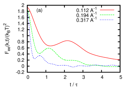
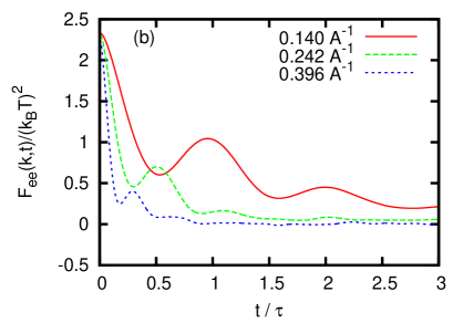
Figure 1: (Color online) Energy density autocorrelation functions $F_{ee}(k,t)$ at three wave numbers as calculated from MD simulations for supercritical Ar at $T=280$ K and densities 750 kg/m³ (a) and 1464.5 kg/m³ (b). The time scales $\tau$ are equal to 3.701 ps (a) and 2.961 ps (b).

Energy density autocorrelation functions $F_{ee}(k,t)=\langle e(k,t)\mathrm{e}^{*}(k,t=0)\rangle$ calculated in MD simulations are shown for three wavenumbers in small-$k$ region in figure 1. The time dependence of these time correlation functions is very similar to the relaxation of the heat density autocorrelations shown in figure 2. A typical feature is an increasing amplitude and a decreasing frequency of the damped oscillations in the shape of $F_{ee}(k,t)$ and $F_{hh}(k,t)$ towards smaller wave numbers, which is typical of the contribution coming from acoustic excitations. The relative strength of the relaxing and oscillating contributions in $F_{hh}(k,t)$ was estimated in the long-wavelength limit in [25] as the inverse of $(\gamma-1)$, i.e., the inverse of the Landau-Placzek ratio known for the density-density time correlation functions. Hence, for the case of the two thermodynamic points of the supercritical Ar studied here and having the experimental ratio of specific heats $\gamma$ of 2.30 and 1.55 [24] for the low- and high-density studied systems, one should observe much smaller relaxing contribution for the low-density state. Indeed, in figure 2 (a) the oscillations in the shape of $F_{hh}(k,t)$ even make the heat density autocorrelation function negative close to $\omega\tau\sim 1$ for the smallest possible in these simulations wave number, while in figure 2 (b), due to the much stronger contribution from the relaxing thermal mode, the $F_{hh}(k,t)$ is positive for all times. It is important that the dimensionless functions $F_{hh}(k,t)$ have the zero-time values tending to the macroscopic values of $C_{\mathrm{v}}$ due to (2.2). Indeed, in figure 2 (a) the zero-time values tend to the macroscopic value of $C_{\mathrm{v}}=1.775$ [24], while for the high-density state they tend to the value $C_{\mathrm{v}}=2.34$.

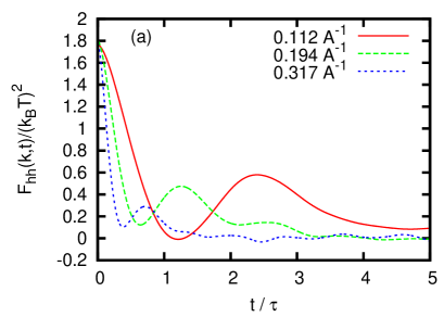
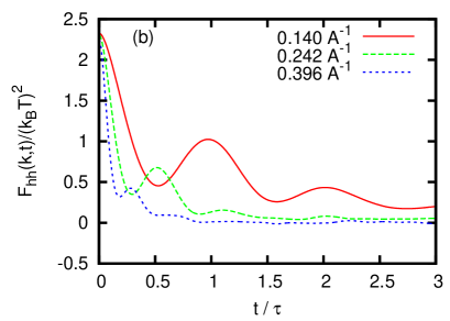
Figure 2: (Color online) Heat density autocorrelation functions $F_{hh}(k,t)$ at three wave numbers as calculated from MD simulations for supercritical Ar at $T=280$ K and densities 750 kg/m³ (a) and 1464.5 kg/m³ (b). The time scales $\tau$ are equal to 3.701 ps (a) and 2.961 ps (b).

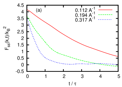
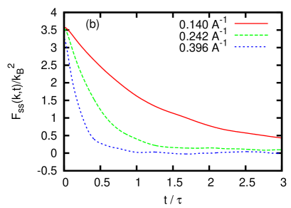
Figure 3: (Color online) Entropy density autocorrelation functions $F_{ss}(k,t)$ at three wave numbers as calculated from MD simulations for supercritical Ar at $T=280$ K and densities 750 kg/m³ (a) and 1464.5 kg/m³ (b). The time scales $\tau$ are equal to 3.701 ps (a) and 2.961 ps (b).

The entropy density autocorrelation functions $F_{ss}(k,t)$ calculated in MD simulations for two densities of the supercritical Ar (figure 3) show for the smallest wave numbers a simple relaxation shape without any oscillating contribution. This is in complete agreement with the prediction of the hydrodynamic theory (2.4). The zero-time values of $F_{ss}(k,t)$ (2.5) should tend in the long-wavelength limit to the macroscopic value of $C_{\mathrm{p}}$. Indeed, one observes in figures 3 (a) and (b) that in agreement with this hydrodynamic prediction, the zero-time values of the normalized functions tend to the macroscopic values of $C_{\mathrm{p}}$ reported in the NIST database: 4.097 for the low-density state and 3.62 for the high-density state.

The time-Fourier transformed energy density (e-e), heat energy density (h-h) and entropy density (s-s) autocorrelation functions, $S_{ii}(k,\omega),~{}i=e,h,s$ are shown for the two studied densities of the supercritical Ar in figure 4. The $S_{ee}(k,\omega)$ and $S_{hh}(k,\omega)$ have the typical of the dynamic structure factors shape with the central peak due to thermal relaxation and the side peak due to propagating acoustic excitations. The ratio of the integral intensities of the central and two side peaks known as the Landau-Placzek-type ratio was obtained in [25] for the case of $S_{hh}(k,\omega)$ and is equal to $(\gamma-1)^{-1}$. The side peak of the $S_{ee}(k,\omega)$ and $S_{hh}(k,\omega)$ is the consequence of the corresponding oscillating contributions to the $F_{ee}(k,t)$ and $F_{hh}(k,t)$, respectively. It is remarkable that the calculated spectral function $S_{ss}(k,\omega)$ shows only the one-peak shape with the central peak due to thermal relaxation (line connected star symbols in figure 4).

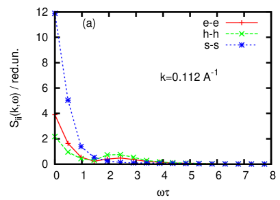
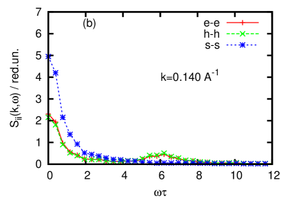
Figure 4: (Color online) Spectral functions energy-energy $S_{ee}(k,\omega)$, heat-heat $S_{hh}(k,\omega)$, entropy-entropy $S_{ss}(k,\omega)$ at the smallest available in MD simulations wave numbers for supercritical Ar at $T=280$ K and densities 750 kg/m³ (a) and 1464.5 kg/m³ (b). The time scales $\tau$ are equal to 3.701 ps (a) and 2.961 ps (b).

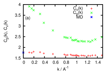
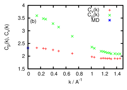
Figure 5: (Color online) Generalized wavenumber-dependent specific heats at constant volume $C_{\mathrm{v}}(k)$ and constant pressure $C_{\mathrm{p}}(k)$ for supercritical Ar at $T=280$ K ad densities 750 kg/m³ (a) and 1464.5 kg/m³ (b). The asterisks at $k=0$ correspond to macroscopic values of $C_{\mathrm{v}}$ calculated from the temperature fluctuations [11].

The zero-time values of the time correlation functions $F_{hh}(k,t)$ and $F_{ss}(k,t)$ permit estimation of the wavenumber-dependent specific heats $C_{\mathrm{v}}(k)$ and $C_{\mathrm{p}}(k)$, which in the long-wavelength limit tend to their macroscopic values. In figure 5 we show the wavenumber dependencies of $C_{\mathrm{v}}(k)$ and $C_{\mathrm{p}}(k)$ for the two densities of the supercritical Ar at temperature 280 K. The asterisks at $k=0$ show the values of macroscopic values of $C_{\mathrm{v}}$ obtained from the standard expression via the thermal fluctuations in the fluid system [11]. One can see that the reported wave-number dependencies tend quite well to the experimental values for the supercritical Ar taken from the NIST database [24]: $C_{\mathrm{v}}$=1.775$k_{\mathrm{B}}$ and $C_{\mathrm{p}}$=4.097$k_{\mathrm{B}}$ for the density of 750 kg/m³ and $C_{\mathrm{v}}$=2.34$k_{\mathrm{B}}$ and $C_{\mathrm{p}}$=3.62$k_{\mathrm{B}}$ for the density of 1464.5 kg/m³.

5 Conclusions

In the MD simulations we calculated the autocorrelation functions of energy density, heat density and energy density and compared them for the smallest available wave numbers with the predictions of the hydrodynamic theory. Our results give evidence of a nice correspondence of the hydrodynamic description of time correlation functions and their zero-time values, which made it possible to estimate the wavenumber-dependent specific heats $C_{\mathrm{v}}(k)$ and $C_{\mathrm{p}}(k)$, with the MD-based estimation of their macroscopic values and experimental values for specific heats of supercritical Ar taken from the NIST database.

These results are very important from the viewpoint of analysing the contributions from thermal relaxation and collective excitations to the specific heats of liquids. Our results and the hydrodynamic approach make evidence of the definitive role of the thermal relaxation in calculation of the specific heats of fluids when it is estimated via dynamic processes. These results will urge a further understanding of the dynamics of the supercritical state of matter, which shows many interesting features observed recently in the scattering experiments and MD simulations on supercritical Argon [29, 30] and Oxygen [31].

Ukrainian 0

Теплоємнiсть рiдин: Гiдродинамiчний пiдхiд Т. Брик${}^{\textsf{\footnotesize{\mbox{?},\penalty 1000\mbox{?}}}}$, Т. Скопiньйо${}^{\textsf{\footnotesize{\mbox{?}}}}$, Дж. Руокко${}^{\textsf{\footnotesize{\mbox{?},\penalty 1000\mbox{?}}}}$

             
${}^{\textsf{\footnotesize 1}}$ Iнститут фiзики конденсованих систем НАН України, 79011 Львiв, Україна ${}^{\textsf{\footnotesize 2}}$ Iнститут прикладної математики та фундаментальних наук, Нацiональний Унiверситет ‘‘Львiвська Полiтехнiка’’, 79013 Львiв, Україна ${}^{\textsf{\footnotesize 3}}$ Фiзичний факультет, Римський унiверситет ‘‘La Sapienza’’, I–00185, Рим, Iталiя ${}^{\textsf{\footnotesize 4}}$ Центр бiо-нано наук Sapienza, Iталiйський технологiчний iнститут, 295 вул. королеви Елени, I–00161, Рим, Iталiя

References

- [1] Hansen J.-P., McDonald I.R., Theory of Simple Liquids, London, Academic, 1986.
- [2] Barker J.A., Henderson D., J. Chem. Phys., 1967, 47, 2856; doi:10.1063/1.1712308.
- [3] Barker J.A., Henderson D., Rev. Mod. Phys., 1976, 48, 587; doi:10.1103/RevModPhys.48.587.
- [4] Weeks J.D., Chandler D., Andersen H.C., J. Chem. Phys., 1971, 54, 5237; doi:10.1063/1.1674820.
-
[5]
Melnyk R., Nezbeda I., Henderson D., Trokhymchuk A.,
Fluid Phase Equilibr., 2009, 279, 1;
doi:10.1016/j.fluid.2008.12.004. - [6] Nezbeda I., Melnyk R., Trokhymchuk A., J. Supercritical Fluid, 2010, 55, 448; doi:10.1016/j.supflu.2010.10.041.
- [7] Kittel Ch., Introduction to Solid State Physics, 8-th Edition, New York, Wiley, 2004.
- [8] Boon J.-P., Yip S., Molecular Hydrodynamics, New-York, McGraw-Hill, 1980.
- [9] Bryk T., Mryglod I., Scopigno T., Ruocco G., Gorelli F., Santoro M., J. Chem. Phys., 2010, 133, 024502; doi:10.1063/1.3442412.
- [10] Bryk T., Eur. Phys. J. Spec. Top., 2011, 196, 65; doi:10.1140/epjst/e2011-01419-x.
- [11] Lebowitz J.L., Perkus J.K., Verlet L., Phys. Rev., 1967, 153, 250; doi:10.1103/PhysRev.153.250.
- [12] Schofield P., Proc. Phys. Soc., 1966, 88, 149; doi:10.1088/0370-1328/88/1/318.
- [13] Schofield P., In: Physics of simple liquids, Temperley H.N.V., Rowlinson J.S., Rushbrooke G.S. (Eds.), North-Holland Publishing, Amsterdam, 1968.
- [14] Copley J.R.D., Lovesey S.W., Rep. Prog. Phys., 1975, 38, 461; doi:10.1088/0034-4885/38/4/001.
- [15] de Schepper I.M., Cohen E.G.D., Bruin C., van Rijs J.C., Montfrooij W., de Graaf L.A., Phys. Rev. A, 1988, 38, 271; doi:10.1103/PhysRevA.38.271.
- [16] Mryglod I.M., Omelyan I.P., Tokarchuk M.V., Mol. Phys., 1995, 84, 235; doi:10.1080/00268979500100181.
- [17] Bryk T., Mryglod I., Phys. Rev. E, 2001, 63, 051202; doi:10.1103/PhysRevE.63.051202.
- [18] Bryk T., Mryglod I., Kahl G., Phys. Rev. E, 1997, 56, 2903; doi:10.1103/PhysRevE.56.2903.
- [19] Bryk T., Ruocco G., Mol. Phys., 2013, 111, 3457; doi:10.1080/00268976.2013.838313.
- [20] Landau L.D., Placzek G., Physik. Z. Sowjetunion., 1934, 5, 172.
- [21] Mountain R.D., Rev. Mod. Phys., 1966, 38, 205; doi:10.1103/RevModPhys.38.205.
- [22] Cohen C., Sutherland J.W.H., Deutch J.M., Phys. Chem. Liq., 1971, 2, 213;doi:10.1080/00319107108083815.
- [23] Bhatia A.B., Thornton D.E., March N.H., Phys. Chem. Liq., 1974, 4, 97;doi:10.1080/00319107408084276.
- [24] Lemmon E.W., McLinden M.O., Friend D.G., Thermophysical Properties of Fluid Systems, In: NIST Chemistry WebBook, NIST Standard Reference Database 69 (National Institute of Standards and Technology, Gaithersburg MD, 2004).http://webbook.nist.gov.
- [25] Bryk T., Ruocco G., Scopigno T., J. Chem. Phys., 2013, 138, 034502; doi:10.1063/1.4774406.
- [26] Woon D.E., Chem.Phys.Lett., 1993, 204, 29; doi:10.1016/0009-2614(93)85601-J.
- [27] Bomont J.-M., Bretonnet J.-L., Pfleiderer T., Bertagnolli H., J. Chem. Phys., 2000, 113, 6815; doi:10.1063/1.1290131.
- [28] Bryk T., Ruocco G., Mol. Phys., 2011, 109, 2929; doi:10.1080/00268976.2011.617321.
- [29] Simeoni G., Bryk T., Gorelli F.A., Krisch M., Ruocco G., Santoro M., Scopigno T., Nat. Phys., 2010, 6, 503; doi:10.1038/nphys1683.
- [30] Gorelli F.A., Bryk T., Krisch M., Ruocco G., Santoro M., Scopigno T., Sci. Rep., 2013, 3, 01203; doi:10.1038/srep01203.
- [31] Gorelli F.A., Santoro M., Scopigno T., Krisch M., Ruocco G., Phys. Rev. Lett., 2006, 97, 245702; doi:10.1103/PhysRevLett.97.245702.
Ukrainian \adddialect\l@ukrainian0 \l@ukrainian