Chemical Abundances in NGC 5053: A Very Metal-Poor and Dynamically Complex Globular Cluster

Abstract

NGC 5053 provides a rich environment to test our understanding of the complex evolution of globular clusters (GCs). Recent studies have found that this cluster has interesting morphological features beyond the typical spherical distribution of GCs, suggesting that external tidal effects have played an important role in its evolution and current properties. Additionally, simulations have shown that NGC 5053 could be a likely candidate to belong to the Sagittarius dwarf galaxy (Sgr dSph) stream. Using the Wisconsin-Indiana-Yale-NOAO-Hydra multi-object spectrograph, we have collected high quality (signal-to-noise ratio $\sim$ 75-90), medium-resolution spectra for red giant branch stars in NGC 5053. Using these spectra we have measured the Fe, Ca, Ti, Ni, Ba, Na, and O abundances in the cluster. We measure an average cluster [Fe/H] abundance of -2.45 with a standard deviation of 0.04 dex, making NGC 5053 one of the most metal-poor GCs in the Milky Way (MW). The [Ca/Fe], [Ti/Fe], and [Ba/Fe] we measure are consistent with the abundances of MW halo stars at a similar metallicity, with alpha-enhanced ratios and slightly depleted [Ba/Fe]. The Na and O abundances show the Na–O anti-correlation found in most GCs. From our abundance analysis it appears that NGC 5053 is at least chemically similar to other GCs found in the MW. This does not, however, rule out NGC 5053 being associated with the Sgr dSph stream.

1. Introduction

Table 1Comparison of NGC 5053 and NGC 5024 (M53) Properties

Cluster	R.A.	Decl.	($l,b$)	$R_{\odot}^{a}$	$R_{\mathrm{GC}}^{a}$	$r_{c}^{b}$	$r_{h}^{b}$	$r_{\mathrm{tr}}^{b}$	c
	(J2000)	(J2000)		(kpc)	(kpc)	(pc)	(pc)	(pc)	$\mathrm{log}(\frac{r_{tr}}{r_{c}})$
NGC 5053	13:16:27.09	+17:42:00.9	$336^{\circ}$,$79^{\circ}$	17.4	17.8	9.71	12.39	89.13	0.96
NGC 5024	13:12:55.24	+18:10:05.4	$333^{\circ}$,$80^{\circ}$	17.9	18.4	2.18	5.84	239.9	2.04

Note. — ^aHarris (1996, Version 2010),^bMcLaughlin & van der Marel (2005)

Globular clusters (GCs) have long served as our laboratories to study the dynamics and evolution of simple stellar populations. With the greater availability of high quality and homogeneous photometric and spectroscopic data, it has become evident that GCs are increasingly complex stellar populations. The Galactic GC population has shown that most GCs exhibit abundance patterns and color-magnitude diagram (CMD) morphology indicative of multiple populations (see e.g., Gratton et al., 2012; Piotto et al., 2014). A number of possible sources for the gas out of which second generation (SG) stars might have formed have been suggested. These sources include rapidly rotating massive stars, massive binary stars, and intermediate-mass AGB stars (see e.g., Ventura et al., 2001; Prantzos & Charbonnel, 2006; D’Ercole et al., 2008, 2010, 2012; de Mink et al., 2009) and all the aspects of the formation, chemical, and dynamical evolution are currently a matter of intensive investigation.

As GCs orbit the Galaxy they are stripped of their stars and help populate the halo. In some instances, wide-field photometric surveys, such as the Sloan Digital Sky Survey (SDSS), have revealed large tidal tails extending from GCs, giving us a snapshot of the tidal stripping experienced by GCs. The most famous of these examples is Palomar 5 (Odenkirchen et al., 2001). Further exploration of SDSS data has revealed that other clusters also show large tidal features. NGC 5053 is one of these clusters (see Lauchner et al., 2006; Jordi & Grebel, 2010).

NGC 5053 is a metal-poor GC located near the north Galactic cap ($l=336^{\circ},b=79^{\circ}$) with a Galactocentric radius of $R_{GC}=17.8$ kpc. Near NGC 5053, $\sim$ 500 pc away based on the X,Y and Z positions from Harris (1996, 2010 version) is NGC 5024 (M53), located at ($l=333^{\circ},b=80^{\circ}$) with a $R_{GC}=18.4$ kpc. A comparison of the physical characteristics of these clusters is given in Table 1. In Figure 1, a history of the previously determined [Fe/H] abundances of NGC 5053 are plotted versus the year of publication. At one point NGC 5053 was considered the most metal-poor GC in the Milky Way (MW) (Zinn, 1985).

Using SDSS photometry, Lauchner et al. (2006) discovered a $6^{\circ}$ tidal tail associated with NGC 5053. A wider field analysis of SDSS photometry, by Jordi & Grebel (2010), confirmed the findings and further mapped the extra-tidal features of the cluster. A study by Chun et al. (2010), using Megacam on the Canada-France-Hawaii Telescope, detected a tidal bridge-like structure between NGC 5053 and its neighbor M53. If this bridge-like structure is genuine, it suggests that the evolution of NGC 5053 has been influenced not only by the Galaxy, but also through interactions with M53. It should be noted that Jordi & Grebel (2010) do not detect this bridge-like structure. The possible complex dynamical history of NGC 5053 does not stop there. Using simulations of the tidal disruption of the Sagittarius dwarf galaxy (Sgr dSph), Law & Majewski (2010) identify NGC 5053 as a likely candidate GC that belongs to the Sgr dSph.

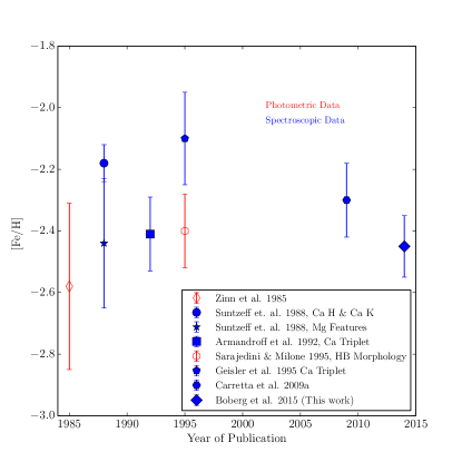
Figure 1.— Previous [Fe/H] determinations for NGC 5053 taken from the literature along with our results. Abundances determined from photometric data are represented by open red markers, and those determined by spectroscopic data are represented by solid blue markers.

Motivated by the apparently complex dynamics of NGC 5053, and its possible association with the Sgr dSph, we have collected high quality spectra of red giant branch (RGB) stars in the cluster. With these spectra we have been able to directly measure the Fe, Ni, Ca, Ti, Na, and O abundances of clusters members in order to determine if NGC 5053 exhibits the typical abundance patterns shown in GCs, such as the Na–O anti-correlation. We will compare these abundances with those seen in other Galactic GCs and field stars at a similar metallicity. We will also present how the abundances in NGC 5053 compare to the abundances in GCs that are generally considered part of the Sgr dSph (M54, Arp 2, Terzan 7, and Terzan 8; see e.g Carretta et al., 2014).

This paper is organized in the following manner. In Section 2 we will present how our observations and data reductions were performed, followed by a description of how cluster members were chosen for this study. In Section 3 we describe how the abundance analysis was carried out and how we assessed the errors in our measurements. The results of our analysis are presented in Section 4. In Section 5 we compare our results for NGC 5053 with abundances in other MW and Sgr GCs and fields stars. We will conclude with possible implications of these abundances and future studies to come.

2. Observations and Data Reduction

2.1. Observations

The spectroscopic data for this study were collected using the Wisconsin-Indiana-Yale-NOAO (WIYN) 3.5 m telescope with the Hydra multi-object spectrograph and a 2600 $\times$ 4000 pixel CCD (STA 1) on 2014 January 18 and 2014 February 14. The Bench Spectrograph was used with the “316@63.4” grating, resulting in spectra with a dispersion of 0.16 Å$\,\mathrm{pixel^{-1}}$ covering a wavelength range of approximately $6063-6380$ Å. The typical signal-to-noise (S/N) ratios of the spectra were 70-90 for the majority of the stars in the sample. In instances where a star was observed in multiple Hydra configurations, once on each of the nights, S/N ratios are on the order of 100. In addition to our program objects, high S/N radial velocity standards were observed at the beginning of each night along with a hot, rapidly rotating B star to use as a template for removing telluric features.

The data were reduced using the standard IRAF software to perform bias subtraction, flat fielding, dark subtraction, and dispersion correction with ThAr comparison lamp spectra. The full integration time (4.5 hr per configuration) was broken up into six separate exposures to reduce the effects of cosmic rays in the final combined spectra. The processed spectra from each exposure were combined using the IRAF task scombine.

2.2. Target Selection

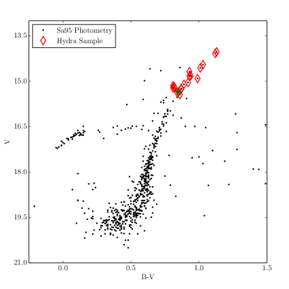
Figure 2.— $V$ vs $(B-V)$ CMD for NGC 5053. Data taken from Sarajedini & Milone (1995). The points overplotted with open diamonds are those stars for which we collected spectra. These are the stars that met the photometric criteria described in the paper. The point plotted as a star marks the location of a star that photometrically appeared to be part of the cluster, but its radial velocity ruled it out as a member.

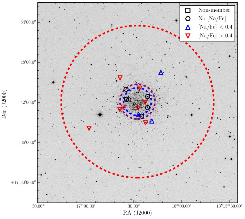
Figure 3.— A Digitized Sky Survey (DSS) image showing NGC 5053. The targets for this study are highlighted by small circles, triangles, and a square. The triangles mark stars for which we were able to measure Na abundances, and the circles mark the stars for which we were not able to do so. The location of the non-member that was observed is marked with a square. The dashed circles represent the core, half-mass, and King truncation radius, respectively, going from smallest to largest. The references for these radii are given in Table 1.

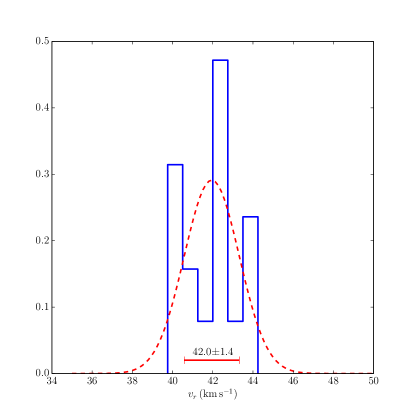
Figure 4.— The radial velocity (RV) distribution of the stars we observed with Hydra. The dashed line in the plot is a normal distribution fit to the histogram shown. The single error bar is centered at the cluster average RV, and the length of the error bar is the standard deviation of the RV sample. The average RV value and standard deviation for the sample are given on top of the the error bar. In measuring the RVs in our sample, we found one field star that met the photometric criteria, but was easy ruled out as a cluster member with an RV of -27.1 $\mathrm{km\,s^{-1}}$.

The stars for this study were selected based on their location on the $B$ vs $(B-V)$ CMD from Sarajedini & Milone (1995), as shown in Figure 2. Our initial sample only included those stars that lie along the RGB in the CMD with a $V\leq 15.5$. At the spectral resolution and high S/N ratio needed to accurately measure abundances, stars fainter than this would require unrealistically long exposure times. The stars that met these criteria, and were observed with Hydra, are represented by open diamonds in Figure 2. A summary of the observational data for our sample is given in Table 2. There we list the positions, photometric values, radial velocities, S/N of the spectra, and cluster membership of each star. The positions of the stars observed in this study are marked on a DSS image of NGC 5053 shown in Figure 3.

Radial velocities were determined for the observed sample using the fxcor task in the NOAO package in IRAF. For each star we measured its radial velocity with four radial velocity standards observed at the beginning of each night. The typical standard deviation of the four individual measurements for a given star was 0.3 $\mathrm{km\,s^{-1}}$ and each measurement had an average error of 2.2 $\mathrm{km\,s^{-1}}$, as estimated by fxcor. We adopted the weighted mean of the four measurements as the final radial velocity value for each star, which is listed in Table 2. The error associated with each velocity in Table 2 is the error on the weighted mean. We also denote which stars are cluster members and which are non-members with a Y and N flag, respectively. The average radial velocity of cluster members is 42.0 $\pm 1.4\,\mathrm{km\,s^{-1}}$. Our sample average radial velocity is in agreement with the previously determined value for the cluster $v_{r}=42.6\pm 0.3\,\mathrm{km\,s^{-1}}$ (Kimmig et al., 2014). The radial velocity distribution of the stars in our sample is shown in Figure 4. The only non-member we observed (Star 22), as listed in Table 2, is not included in Figure 4 because it sits too far away from the cluster distribution, and would skew the x-axis of the plot.

Table 2Observational Data

ID	R.A.	Decl.	$V$	$M_{v}$	$(B-V)_{0}$	$(V-K)_{0}$	$v_{r}$	$\sigma_{v_{r}}$	S/N	Member
	J2000	J2000					($\mathrm{km\,s^{-1}}$)	($\mathrm{km\,s^{-1}}$)		Y/N
2	13:16:26.71	+17:41:01.6	14.03	-2.23	1.09	2.71	44.2	0.8	83	Y
3	13:16:12.23	+17:46:22.9	14.08	-2.18	1.08	2.73	44.0	1.0	70	Y
4	13:16:20.60	+17:42:46.4	14.45	-1.81	0.99	2.58	42.2	0.8	82	Y
6	13:16:35.95	+17:41:12.8	14.56	-1.70	0.97	2.55	42.2	0.6	108	Y
9	13:16:26.45	+17:40:07.6	14.68	-1.58	0.89	2.41	43.8	1.1	108	Y
10	13:16:24.50	+17:39:50.0	14.82	-1.44	0.90	2.44	40.6	1.8	50	Y
11	13:16:57.64	+17:38:05.1	14.83	-1.43	0.89	2.43	40.5	0.7	71	Y
12	13:16:38.19	+17:40:51.8	14.91	-1.35	0.95	2.51	42.3	1.0	109	Y
14	13:16:37.90	+17:45:35.5	15.04	-1.22	0.88	2.39	40.1	1.2	80	Y
15	13:16:20.74	+17:41:05.9	15.10	-1.16	0.85	2.36	43.1	0.9	83	Y
16	13:16:25.56	+17:44:02.3	15.15	-1.11	0.77	2.20	42.6	1.4	79	Y
17	13:16:18.18	+17:39:05.7	15.19	-1.07	0.78	2.20	42.6	1.2	121	Y
18	13:16:32.51	+17:42:17.4	15.22	-1.04	0.77	2.16	41.7	1.1	60	Y
19	13:16:34.20	+17:43:53.1	15.24	-1.02	0.83	2.27	40.8	0.8	70	Y
20	13:16:22.27	+17:41:53.6	15.25	-1.01	0.83	2.53	42.1	0.8	82	Y
21	13:16:22.13	+17:38:50.1	15.26	-1.00	0.83	2.31	40.3	1.2	73	Y
22	13:16:28.55	+17:41:12.6	15.35	-0.91	0.81	1.82	-27.1	0.7	80	N
23	13:16:33.91	+17:42:22.9	15.37	-0.89	0.80	2.26	39.7	1.4	64	Y

Table 3Derived Atmospheric Parameters

ID	$T_{eff}$	$BC_{v}$	log(g)	$v_{t}$
	K		$\mathrm{cm\,s^{-2}}$	$\mathrm{km\,s^{-1}}$
2	4460	-0.53	0.80	1.67
3	4400	-0.55	0.80	1.73
4	4500	-0.48	1.10	1.67
6	4580	-0.46	1.10	1.85
9	4660	-0.42	1.20	1.85
10	$\cdots$	$\cdots$	$\cdots$	$\cdots$
11	4570	-0.46	1.20	2.00
12	4490	-0.51	1.20	2.08
14	4630	-0.44	1.40	1.65
15	4630	-0.43	1.40	2.09
16	4760	-0.38	1.50	1.80
17	4750	-0.39	1.50	1.41
18	4850	-0.35	1.69	1.34
19	4650	-0.43	1.40	1.65
20	4700	-0.33	1.50	2.11
21	4680	-0.41	1.50	1.19
22	$\cdots$	$\cdots$	$\cdots$	$\cdots$
23	4700	-0.41	1.50	1.50

3. Analysis

3.1. Atmospheric Parameters

Initial estimates of the atmospheric parameters ($T_{eff},BC_{v}$) were determined from the $B,V,I$ photometry (Sarajedini & Milone, 1995) and 2MASS $J,H,K$ for each star using the relations found in Alonso et al. (1999), using the $(B-V)$, $(V-K)$, $(J-H)$, and $(J-K)$ colors. The colors were dereddened with an E(B-V) = 0.04 (Lauchner et al., 2006), which is a consistent value across the literature, following the relations found by Rieke & Lebofsky (1985). Surface gravities were calculated based on the derived effective temperatures and bolometric corrections assuming a mass of $0.8M_{\odot}$ for every star in the sample and a distance modulus of $(m-M)_{V}=16.26$ (Sarajedini et al., 2007). Due to the limited number of measurable Fe I and Fe II lines in our spectral region, it was not possible to adjust the $T_{\mathrm{eff}}$ and log($g$) from their photometrically determined values using excitation or ionization equilibrium.

The microturbulent velocity ($v_{t}$) of each star was determined using the relationships found in Carretta et al. (2004), Johnson et al. (2008), and Pilachowski et al. (1996). The initial estimate of $v_{t}$ was an average of the velocities resulting from the relations found in the three references listed above. The $v_{t}$ was later adjusted to minimize the dependence of derived [Fe/H] abundance on Fe I line strength. The final adopted atmospheric parameters are listed in Table 3. MARCS LTE model atmospheres (Gustafsson et al., 2008) were interpolated to the photometrically determined atmospheric parameters in order to be used in the abundance measurements. We did not derive these stellar parameters for Star 10 because its spectrum was too noisy to use for abundances measurements. Star 22 is also listed without these parameters because it was determined to not be a cluster member from its radial velocity.

3.2. Equivalent Width (EW) Measurements

The iron (Fe), nickel (Ni), titanium (Ti), and calcium (Ca) abundances in our sample were determined from EW measurements of individual Fe I, Ni I, Ti I and Ca I lines, respectively. The spectra in our sample were compared to a high resolution solar spectrum (Wallace et al., 2011) to confirm the location of lines and possible blends. EWs were measured using the splot task in IRAF on the continuum-normalized spectra. The final line lists were complied with log($gf$) values and excitation potentials taken from the Gaia-ESO Survey (Heiter et al. in prep). The EW measurements and atomic parameters for all lines used are available electronically. The abundances were determined using the abfind task in the 2010 August version of MOOG (Sneden, 1973). We assumed the solar abundances as found by Anders & Grevesse (1989).

Table 4Equivalent Widths

Element	$\lambda$	log($gf$)	EP	EW
	(Å)		(eV)	(mÅ)
Fe I	6136.61	-1.402	2.45	99.9
Fe I	6136.99	-2.950	2.20	32.2
Fe I	6137.69	-1.402	2.59	999.9
Fe I	6151.62	-3.295	2.18	21.6
Fe I	6173.33	-2.880	2.22	36.1

Note. — Table 4 is published in its entirety in the electronic edition of the Astrophysical Journal. A portion is shown here for guidance regarding its form and content. The full version contains all the lines for the other 17 stars.

3.3. Spectral Synthesis

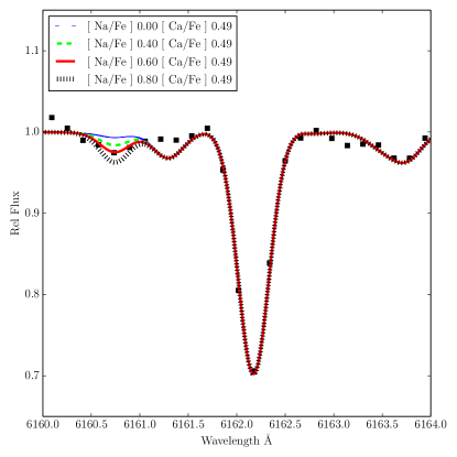
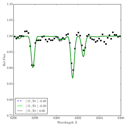
Figure 5.— An example of the spectral synthesis performed to determine the Na and O abundances for Star 6. Left panel: the spectral region around the Na I line near 6160 Å. The strong line located at approximately 6162 Å  is a Ca I line. Right panel: the spectral window near the [O I] line near 6300 Å. In each panel the data are plotted as black squares. The spectrum in the right hand panel has been corrected for telluric features.

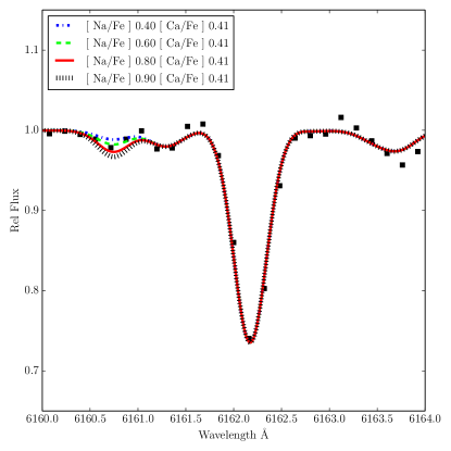
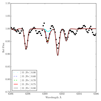
Figure 6.— As in Figure 5, but for Star 12 with similar atmospheric parameters but very different oxygen abundance.

The sodium (Na), oxygen (O), and barium (Ba) abundances were determined using spectral synthesis to account for blends, molecular bands, and in the case of Ba, hyperfine structure and the isotopic mix of the element. Synthetic spectra were generated using the synth task in MOOG, with MARCS model atmospheres that matched the atmospheric parameters of each star, and an [Fe/H] abundance as determined through EW measurements. Assuming Gaussian broadening, the FWHM of the synthetic spectral lines was set to match the FWHM of unblended lines in the observed spectra. The final abundances were determined by creating synthetic spectra with a range of abundances for the species and line in question, and choosing the synthesis that best matched the observed spectra. An error was assigned to these abundances by determining how much the abundance could be varied before the synthetic spectrum would greatly deviate from the observed lines. Examples of the spectral synthesis are shown in Figure 5 and Figure 6.

In our spectral region, there are two Na I lines that we used to determine the [Na/Fe] abundance at $6154$ Å  and $6160$ Å. For many of the stars, the line at $6154$ Å  was too weak to measure and the final [Na/Fe] abundances were based on the single line at $6160$ Å. In the cases where both lines were present, an average of the [Na/Fe] resulting from each line was used as the final abundance. There were also cases where both of these lines were too noisy to determine an [Na/Fe] abundance for the star. In total, we were able to determine the [Na/Fe] abundance in 11 of the 18 stars observed.

Oxygen abundances were determined from the [O I] line at $6300$ Å. In this region of the spectrum there is a significant amount of contamination from telluric features. To remove these features, we divided the observed spectrum by the scaled spectrum of a hot B star, which acted as our template for the telluric features. The synthetic spectra were then compared to these telluric corrected spectra when determining the final [O/Fe] abundances. As a test, we also determined the [O/Fe] abundances from uncorrected spectra and there were no differences in the results. This indicated to us that the [O I] line was not significantly affected by the neighboring telluric lines. There is also a strong night sky emission line near this [O I] feature. The radial velocity shift of the NGC 5053 stars moved the sky line off of the [O I] feature. In some cases, however, the strength of the sky line varied enough so that the sky subtraction was not good enough to completely remove the line. In these cases the residual from the sky line was large enough to affect the [O I] feature. It is for that reason that we were only able to measure [O/Fe] abundances in 8 stars.

The [Ba/Fe] abundances were determined from the Ba II line at $6141$ Å. In order to create an accurate synthetic spectrum including this feature, we had to assume an isotopic mix of Ba. This is complicated by the fact that Ba is both an s- and r-process neutron capture element. At low metallicities, such as those in NGC 5053, the Ba production is thought to be dominated by the r- process because of the slower timescales over which the s-process would contribute to the overall Ba production. Following the work of McWilliam (1998), we only considered the following isotopes ${}^{135}\mathrm{Ba},^{137}\mathrm{Ba},^{138}\mathrm{Ba}$, with a ratio of $40:32:28$, respectively. We also adopt the r-process solar composition of $\mathrm{log}(\epsilon_{\odot}(\mathrm{Ba})_{r})=1.46$, as found by McWilliam (1998). It should be noted that there is an Fe I line at $6140$ Å  which can blend with the Ba II line, resulting in inaccurate [Ba/Fe] abundance determinations. At the metallicity of NGC 5053, however, the line is very weak so the effect is minimal.

3.4. Uncertainties

To quantify the errors in our abundance measurements, we determined how much the abundances changed with variations in the atmospheric parameters of a given model. New models were generated with one of the atmospheric parameters varying, while the others were held constant. The abundance analysis was then repeated with these new models until we had sampled a sufficient grid of the parameter space to assess the errors induced by their individual uncertainties. A summary of this error analysis is given in Table 5. The analysis was performed on a star with the following atmospheric parameters over the range indicated with each value: $T_{eff}=4760\pm 100$ (K), $\mathrm{log}$ $g$, = 1.50 $\pm 0.2$ (cgs), [M/H] = -2.5 $\pm 0.2$ (dex),$v_{t}$ = 1.8 $\pm 0.2\,\mathrm{km\,s^{-1}}$.

In Table 5 we list the $\sigma_{\mathrm{obs.}}$ and $\sigma_{\mathrm{total}}$ for each abundance measured. For abundances determined using EWs, $\sigma_{\mathrm{obs.}}$ is the standard deviation of abundances determined from the number of lines listed in the table. In cases where only one line was measured this field is left blank. For those abundances that were determined with spectral synthesis (Na, O, Ba), $\sigma_{\mathrm{obs.}}$ is the error assigned to each abundance as described in the previous section. To calculate $\sigma_{\mathrm{total}}$, we added the uncertainties from the atmospheric parameters in quadrature. From this analysis we see that our observed uncertainty is consistent with that expected from variations in atmospheric parameters.

Table 5Uncertainties on Atmospheric Parameters

Ion	$T_{eff}\,\pm 100$	log $g\,\pm 0.20$	[M/H] $\,\pm 0.10$	$v_{t}\,\pm 0.25$	$\sigma_{\mathrm{total}}$	No.	$\sigma_{\mathrm{obs}}$
	(K)	(cgs)	(dex)	($\mathrm{km\,s^{-1}}$)	(dex)	Lines	(dex)
Fe I	$\pm 0.13$	$\pm 0.02$	$\pm 0.02$	$\mp 0.03$	0.14	9	0.07
$[\mathrm{OI}]$	$\pm 0.10$	$\pm 0.07$	$\pm 0.02$	$\pm 0.00$	0.12	1	0.20
Na I	$\pm 0.10$	$\pm 0.07$	$\pm 0.02$	$\mp 0.05$	0.13	1	0.20
Ca I	$\pm 0.11$	$\pm 0.03$	$\pm 0.01$	$\mp 0.07$	0.13	3	0.09
Ti I	$\pm 0.12$	$\pm 0.01$	$\pm 0.01$	$\mp 0.01$	0.12	1	$\cdots$
Ni I	$\pm 0.13$	$\pm 0.01$	$\pm 0.01$	$\mp 0.01$	0.13	1	$\cdots$
Ba II	$\pm 0.07$	$\pm 0.05$	$\pm 0.05$	$\mp 0.05$	0.11	1	0.20

4. Results

4.1. Fe, Ca, Ti, Ni, Ba

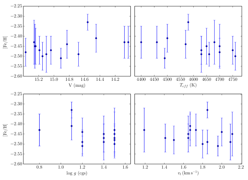
Figure 7.— [Fe/H] as a function of apparent magnitude $V$, $T_{\mathrm{eff}}$, log($g$), and $v_{t}$. The vertical error bars in each of the plots represent the standard deviation of the [Fe/H] abundance of a given star.

In Figure 7 we plot the [Fe/H] abundance as a function of V, $T_{\mathrm{eff}}$, log($g$), and $v_{t}$ for each star to see if there are trends in the measured [Fe/H] values with these parameters. The error bars in the vertical direction represent the standard deviation of the [Fe/H] values given by the Fe I lines in a given spectrum. We do not find any trends in [Fe/H] with any of these parameters.

The individual stellar abundances for Fe, Ca, Ti, Ni, and Ba are given in Table 6 with the number of lines averaged together to reach the final abundance. In the second to last row of Table 6 we list the the average cluster abundance for Fe, Ca, Ti, Ni, and Ba with the number of stars used in the average and the standard deviation of the measurements. The final row of Table 6 lists the assumed solar abundances used to calculate the abundance ratios given in this table. In Figure 8 we present a box- and -whisker plot of the Ca, Ti, Ni and Ba abundances to illustrate the median cluster abundance of these species, as well as their individual distributions in the cluster.

Table 6Fe, Ca, Ti, Ni, and Ba Abundances in NGC 5053

ID	[Fe/H]	$\sigma_{\mathrm{Fe}}$	n	[Ca/Fe]	$\sigma_{\mathrm{Ca}}$	n	[Ti/Fe]	$\sigma_{\mathrm{Ti}}$	n	[Ni/Fe]	$\sigma_{\mathrm{Ni}}$	n	[Ba/Fe]	$\sigma_{\mathrm{Ba}}$	n
2	-2.43	0.08	17	0.60	0.06	5	0.49	$\cdots$	1	-0.06	0.15	2	-0.58	0.1	1
3	-2.43	0.08	11	0.46	0.01	2	0.32	0.11	3	$\cdots$	$\cdots$	1	-0.33	0.1	1
4	-2.41	0.07	11	0.43	0.00	2	0.09	0.14	2	0.07	0.31	2	-0.58	0.2	1
6	-2.33	0.04	10	0.49	0.04	4	0.26	0.02	2	-0.26	0.02	2	-0.58	0.2	1
9	-2.49	0.06	12	0.44	0.07	6	$\cdots$	$\cdots$	$\cdots$	-0.07	$\cdots$	1	-0.58	0.2	1
10	$\cdots$	$\cdots$	$\cdots$	$\cdots$	$\cdots$	$\cdots$	$\cdots$	$\cdots$	$\cdots$	$\cdots$	$\cdots$	$\cdots$	$\cdots$	$\cdots$	$\cdots$
11	-2.44	0.07	8	0.32	0.07	3	0.28	0.22	2	0.02	$\cdots$	1	-0.58	0.1	1
12	-2.51	0.08	13	0.41	0.07	4	0.19	0.07	2	0.02	$\cdots$	1	-0.53	0.2	1
14	-2.47	0.07	9	0.51	0.14	5	0.39	$\cdots$	1	0.15	$\cdots$	1	-0.78	0.2	1
15	-2.48	0.09	13	0.32	0.05	2	0.32	0.20	2	-0.15	$\cdots$	1	-0.58	0.2	1
16	-2.50	0.07	9	0.51	0.09	3	0.56	$\cdots$	1	0.3	$\cdots$	1	-0.43	0.2	1
17	-2.47	0.07	9	0.42	0.09	6	$\cdots$	$\cdots$	$\cdots$	$\cdots$	$\cdots$	$\cdots$	-0.58	0.1	1
18	$\cdots$	$\cdots$	$\cdots$	$\cdots$	$\cdots$	$\cdots$	$\cdots$	$\cdots$	$\cdots$	$\cdots$	$\cdots$	$\cdots$	$\cdots$	$\cdots$	$\cdots$
19	-2.45	0.09	11	0.62	0.06	2	0.32	0.15	2	0.28	$\cdots$	1	-0.43	0.1	1
20	-2.45	0.11	13	0.43	0.12	3	$\cdots$	$\cdots$	$\cdots$	0.15	$\cdots$	1	-0.53	0.1	1
21	-2.43	0.11	13	0.5	0.16	5	0.27	$\cdots$	1	0.13	$\cdots$	1	-0.53	0.1	1
22	$\cdots$	$\cdots$	$\cdots$	$\cdots$	$\cdots$	$\cdots$	$\cdots$	$\cdots$	$\cdots$	$\cdots$	$\cdots$	$\cdots$	$\cdots$	$\cdots$	$\cdots$
23	-2.48	0.07	8	0.39	0.18	4	0.43	0.21	2	0.00	0.01	2	-0.43	0.1	1
Cluster Avg.	-2.45	0.04	15	0.45	0.08	15	0.32	0.11	12	0.03	0.14	13	-0.54	0.1	15
$\mathrm{log}(\epsilon_{\odot})$	7.52			6.36			4.99			6.25			2.13

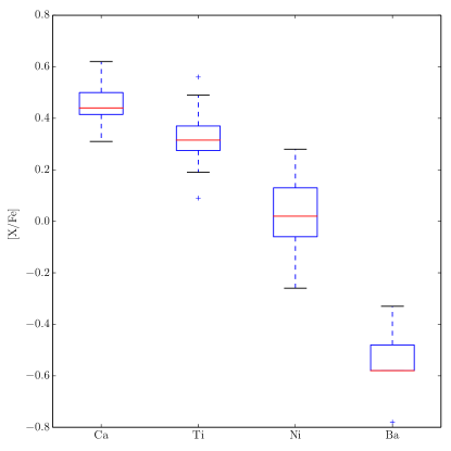
Figure 8.— Box- and- whisker plot of the Ca, Ti, Ni and Ba abundances in NGC 5053. The red line is the median of each abundance, the bottom of each box is the first quartile, the top of each box is the third quartile, and the caps represent the minimum and maximum values.

Table 7Na and O Abundances in NGC 5053

ID	$[\mathrm{Na/Fe}]$	Error	$[\mathrm{O/Fe}]$	Error
2	0.7	0.2	0.2	0.2
3	$<0.0$	$\cdots$	0.3	0.2
4	$\cdots$	$\cdots$	0.6	0.2
6	0.6	0.20	-0.2	0.2
9	$<0.0$	$\cdots$	0.4	0.2
10	$\cdots$	$\cdots$	$\cdots$	$\cdots$
11	1.0	0.2	$\cdots$	$\cdots$
12	0.6	0.2	0.75	0.1
14	0.8	0.3	$\cdots$	$\cdots$
15	$\cdots$	$\cdots$	$\cdots$	$\cdots$
16	0.9	0.3	$<0.2$	$\cdots$
17	0.0	0.2	0.4	0.2
18	$\cdots$	$\cdots$	$\cdots$	$\cdots$
19	$\cdots$	$\cdots$	$\cdots$	$\cdots$
20	0.9	0.2	$\cdots$	$\cdots$
21	0.8	0.2	$\cdots$	$\cdots$
22	$\cdots$	$\cdots$	$\cdots$	$\cdots$
23	$\cdots$	$\cdots$	$\cdots$	$\cdots$

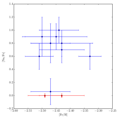
Figure 9.— The individual [Na/Fe] abundances for each star plotted vs their respective [Fe/H] abundance. This plot shows that there are two separate groups of [Na/Fe] abundances present in our sample.

4.2. Na and O

Using spectral synthesis we were able to determine the Na abundance in 11 of the 18 stars in our sample, and the O abundance in 8 of them. There were 7 stars which had both Na and O abundances measured. These abundances are summarized in Table 7. The [Na/Fe] versus [Fe/H] abundance for each star and the [Na/Fe] distribution for the cluster are plotted in Figure 9 and Figure 10, respectively. In Figure 10, the solid black line is a generalized histogram of the [Na/Fe] values. The generalized histogram was created by treating each measurement as a Gaussian with a standard deviation equal to the error on that measurement. These individual Gaussians were then added together to produce the distribution shown in Figure 10 by the solid line. The distribution represented by this generalized histogram is best fit by two Gaussians centered at [Na/Fe] = –0.03 dex and [Na/Fe] = 0.78 dex, with standard deviations of 0.30 and 0.28, respectively. From these figures we clearly see that there is a spread on the order of 0.8 dex in the [Na/Fe] distribution of our sample, which is larger than the expected errors on the measurements.

5. Discussion

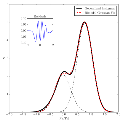
Figure 10.— Generalized histogram of the [Na/Fe] abundances. The thick dashed line is the two-peaked Gaussian fit to this distribution, with the individual Gaussian components plotted as thin dashed lines. The residuals between the fit and the generalized histogram are shown in the upper left-hand corner.

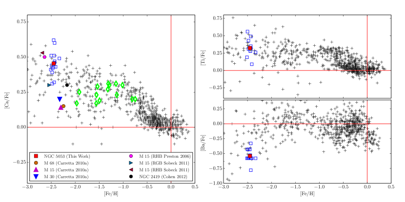
Figure 11.— The Ca, Ti, and Ba abundances of the stars in our sample plotted with a Milky Way Sample taken from Venn et al. (2004), plotted as black crosses. The open squares in each plot represent the individual abundances for the individual stars in our sample, the solid red square marks the average of these individual abundances. Left panel: the open diamonds are Milky Way GC abundances as measured by Carretta et al. (2010a) for Ca. Also on this plot, are additional measurements for M15, with references given in the legend. While M15, M68, and M30 are from the Carretta et al. (2010a) sample, they are given different markers to highlight their values in relationship to NGC 5053.

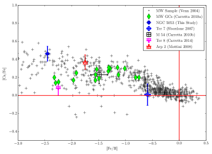
Figure 12.— A comparison of the NGC 5053 [Ca/Fe] abundance with the GCs traditionally thought to be associated with the Sgr dSph: M54, Arp 2, Terzan 7, and Terzan 8.

5.1. Comparison With MW

With the abundances that we determined, we can place NGC 5053 in the context of the chemical composition of stars in the MW. To make this comparison, in Figure 11 we plot the [Ca/Fe], [Ti/Fe], and [Ba/Fe] abundances of NGC 5053 with a MW sample taken from Venn et al. (2004). In these plots the Venn et al. (2004) sample is plotted as black crosses. For each species, the individual cluster members of NGC 5053 are plotted as open squares and the cluster average for that species is plotted as a filled square. From these plots we can see that NGC 5053 lies within the envelope defined by MW stars at a similar metallicity. Specifically, the alpha-elements in our sample, [Ca/Fe] and [Ti/Fe], are enhanced by typical amounts while the [Ba/Fe] is depleted. The large spread in the [Ti/Fe] abundances comes from the fact that the TiI lines were relatively weak and in many cases only 1 or 2 lines were available in our spectral window.

On the [Ca/Fe] vs [Fe/H] plot we include the [Ca/Fe] abundances for other GCs in the MW. The open green diamonds mark the abundances as found by Carretta et al. (2010a). The abundances for M68, M15, and M30 from the Carretta et al. (2010a) sample are given different markers to highlight the locations of the three most metal-poor GCs in their sample. In addition to the their sample, we include two other measurements of M15 from Preston et al. (2006) and Sobeck et al. (2011), and the abundances for NGC 2419 as found by Cohen & Kirby (2012). The abundance ratios from other studies have been adjusted to our assumed solar values.

From the [Ca/Fe] panel in Figure 11, it would appear that NGC 5053 is more similar to the MW field population than the GC sequence populated by the Carretta et al. (2010a) sample. It is difficult, however, to know if this offset is real or caused by the systematic differences between different studies. The abundances plotted for M15 illustrate this point well. Between the four measurements for M15 on this panel, [Fe/H] ranges from -2.3 to -2.64 and [Ca/Fe] ranges from 0.11 to 0.53. In the case of Sobeck et al. (2011) the difference in abundances could arise from the evolutionary state of the stars being studied, but this could not account for the larger offsets shown in the plot. Potential systematic differences in abundance analyses can arise from a multitude of effects, including different measurement and analysis techniques, adopted stellar models, stellar atmospheric parameters, and atomic parameters. The samples collected to make this plot did have a few Ca I and Fe I lines in common with our work and these had identical log($gf$) values, but most lines were unique to each study. With these considerations in mind, we can say that NGC 5053 exhibits alpha enhancement that is typical of MW field stars and GCs at a similar metallicity and is among the most metal-poor GCs in the MW.

5.2. Comparison with Sgr dSph GCs

Throughout the literature, M54, Arp 2, Terzan 7, and Terzan 8 are considered to be GCs that originated from the Sgr dSph, with M54 being at the nucleus of the dwarf galaxy (see Ibata et al., 1994; Da Costa & Armandroff, 1995; Law & Majewski, 2010). In Figure 12 we plot the [Ca/Fe] of NGC 5053 along with these four clusters versus their respective [Fe/H] abundances. Also plotted is the MW star sample from Venn et al. (2004). In this figure all of the abundances have been adjusted to our assumed solar values. As mentioned earlier and demonstrated in Figure 11, the apparent offset of some of the Sgr dSph GCs from the MW GC sequence could be due to the systematic differences between the studies. In general, the GCs considered to be members of the Sgr dSph do not show [Ca/Fe] values that are drastically different from either the MW GC sequence or the field stars at their respective metallicities, despite the systematic differences between studies. If NGC 5053 were to be confirmed as a member of the Sgr dSph it would be the most metal-poor cluster known to date.

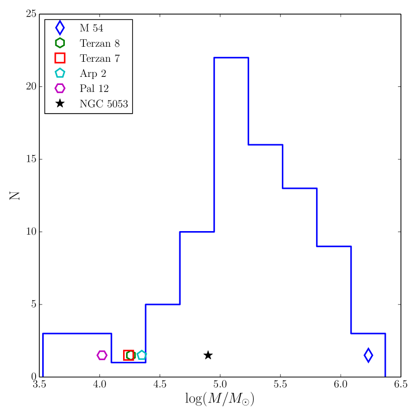
Figure 13.— Distribution of GC masses in the Milky Way. The locations of the 4 Sgr dSph GCs are marked in the distribution with open points and NGC 5053 is marked with a filled star symbol. The distribution was taken from McLaughlin & van der Marel (2005).

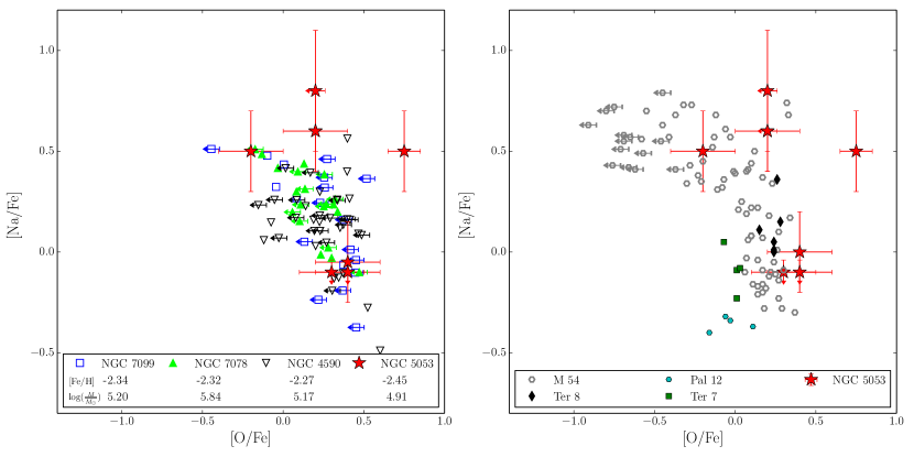
Figure 14.— Left panel: plot of the [Na/Fe] vs. [O/Fe] abundances in NGC 5053, NGC 7099, NGC 7078, NGC 4590. The [Fe/H] abundance and mass for each cluster is given in the plot legend. Right panel: plot of [Na/Fe] vs. [O/Fe] for NGC 5053 and other Sgr dSph candidate GCs. The abundances for M54, Pal 12, Terzan 7, and Terzan 8 were taken from Carretta et al. (2010b), Cohen (2004), Sbordone et al. (2007), and Carretta et al. (2014), respectively. All of the abundances have been put on our abundance scale and corrected for NLTE affects.

NGC 5053 would also be a relatively high-mass GC member of the Sgr dSph. Plotted in Figure 13 is the distribution of GC masses in the MW. The locations of M54, Arp 2, Terzan 7, Terzan 8, Pal 12 and NGC 5053 are marked on the distribution. The MW GC distribution shown in this plot results from the King model masses reported by McLaughlin & van der Marel (2005). The individual masses marked on the distribution were calculated based on their respective absolute magnitudes reported in Harris (1996, Version 2010) and a mass-to-light ratio of $M/L=2$. We used these calculated masses so that the individual clusters would be on a consistent scale. It should be noted that recent work by Salinas et al. (2012) and Sollima et al. (2014) report the mass of Terzan 8 to be slightly higher at $\mathrm{log}(M/M_{\odot})=$ 4.5 and 4.93, respectively. The result by Sollima et al. (2014) would give Terzan 8 a mass approximately equal to, or slightly larger, than NGC 5053. This figure shows that NGC 5053 would be the second most massive GC associated with the Sgr dSph, after M54.

5.3. Na–O Anti-correlation

As stated earlier, it was only possible to measure the [Na/Fe] and [O/Fe] abundances for seven of the stars in our sample. Despite this limited sample, NGC 5053 still exhibits an abundance pattern in these species that is consistent with the Na–O anti-correlation found in other clusters with larger samples, such as M54. In the left-hand panel of Figure 14, we plot the [Na/Fe] vs [O/Fe] abundances for NGC 5053 and clusters of similar metallicity (NGC 7099, NGC 7078, NGC 4590) from Carretta et al. (2009a). This panel shows that the extent of the Na–O anti-correlation present in NGC 5053 is consistent with that found in other metal-poor MW GCs. In the right-hand panel of Figure 14 we plot the [Na/Fe] and [O/Fe] abundances for NGC 5053 and the Sgr dSph clusters M54, Pal 12, Terzan 7, and Terzan 8. Pal 12 is an additional cluster that is considered to be a likely candidate associated with the Sgr dSph by Law & Majewski (2010). The abundances from other studies have been placed on our assumed solar scale and the [Na/Fe] abundances have been corrected for NLTE effects following the models in Gratton et al. (1999). From this panel, we see that Terzan 7, Terzan 8, and Pal 12 do not show an extended Na–O anti-correlation and appear to be composed mostly, or entirely, of a single, first generation (FG) of stars. Carretta et al. (2014) suggest that Terzan 8 is a GC composed of mostly FG stars, with only 1 star in their sample appearing to belong to the SG. The size of our sample of NGC 5053 stars with Na and O abundances is comparable to the Carretta et al. (2014) sample, with 7 and 6 respectively. The NGC 5053 sample, however, shows signs of a more extended Na–O anti-correlation and a larger fraction of stars in the SG. This panel also shows that the apparent FG of stars in NGC 5053 has [Na/Fe] abundances consistent with those in Pal 12, Terzan 7, and Terzan 8.

With so few stars in the sample it is difficult to put constraints on how to divide the sample into the FG and SG stars. Based on the [Na/Fe] distribution shown in Figure 10, an [Na/Fe] abundance of $\sim 0.4$ roughly divides the double peaked Gaussian distribution into its two components, with an [Na/Fe] $<0.4$ being the FG and [Na/Fe] $>0.4$ being the SG of stars. Following this separation criterion, our sample would contain 3 FG stars and 8 SG stars. The fractions of FG and SG stars in NGC 5053 are consistent with those found in other MW GCs (Carretta et al., 2009b). In Figure 3, we show the distribution of these stars on the cluster field; the FG stars are marked with blue triangles pointing up, and the SG stars are marked with red triangles pointing down. Unfortunately, there were too few stars to explore the radial distribution of the different generations in the cluster. Out of the 5 GCs plotted in Figure 14, NGC 5053 is the second most massive, after M54. In this less massive Sgr dSph candidate GC sample, NGC 5053 is the only GC to show signatures of SG stars. While this does not put any constraints on the likelihood that NGC 5053 is a Sgr dSph cluster, it does illustrate how cluster mass affects and balances the presence of multiple generations.

A study by Smolinski et al. (2011) found that NGC 5053 cluster members have an approximately unimodal CN band strength distribution, suggesting only FG stars are in the cluster. While their result my seem to contradict what we find in NGC 5053, this is not the case. As noted by Smolinski et al. (2011) and Shetrone et al. (2010), their analysis of CN and CH molecular bands is limited by the [Fe/H] of the clusters. At low metallicities, such as those found in NGC 5053, the variations in these molecular band strengths will become difficult to detect, causing clusters to appear to be chemically homogeneous in light element abundances. This leads them to conclude that a low metallicity cluster showing a unimodal band strength distribution could still have chemical inhomogeneities and multiple populations in the cluster.

6. Conclusions

NGC 5053 is possibly a very dynamically complex GC in our Galaxy. Not only has this cluster been shown to have significant tidal tails, but one study has also detected a tidal bridge with the neighboring cluster M53. The already rich dynamical environment of NGC 5053 is further complicated by its possible association with the Sgr dSph. The goal of this study was to determine if NGC 5053 shows the typical chemical signatures of MW GCs by collecting high quality spectra for a sample of RGB stars in the cluster. By using both EW measurements and spectral synthesis, we have been able to determine the Fe, Ca, Ti, Ni, Ba, Na, and O abundances in NGC 5053.

The abundance results are summarized as follows:

1. The cluster average [Fe/H] = -2.45 from 15 stars, with $\sigma=0.04$, making NGC 5053 one of the most metal-poor GCs in the Galaxy.

2. From our target selection we determine the radial velocity of the cluster to be $v_{r}=42.0\pm 1.4$ $\mathrm{km\,s^{-1}}$.

3. At this metallicity, the [Ca/Fe], [Ti/Fe], and [Ba/Fe] abundances are consistent with the abundances found for halo stars in the MW. Specifically, the $\alpha$-elements are enhanced and the Ba is depleted, relative to solar.

4. The Na and O abundances exhibit star-to-star variations within our sample. These variations are larger than the typical uncertainty in their respective measurements. The [Na/Fe] distribution is well fit by two Gaussians with mean values separated by 0.8 dex. The Na and O abundances exhibit a distribution that is consistent with other GCs in the MW. From these abundances, NGC 5053 appears to have both a FG and a SG of stars still present in the cluster. The relative fraction of FG and SG stars in our sample for NGC 5053 is consistent with other GCs in the MW. The extent of the Na-O anti-correlation in NGC 5053 is similar to what is seen in other metal-poor MW GCs, specifically M15, M68, and M30.

5. Like the other Sgr dSph candidate GCs, NGC 5053 appears chemically similar (e.g., alpha-enhanced) to the MW field population at a similar metallicity. Unlike MW GCs, however, the other Sgr dSph GC candidates do not show an extended Na–O anti-correlation or clear signs of multiple populations, apart from M54. Out of the candidate GCs with abundances we pulled from the literature, NGC 5053 is the most massive, after M54, and shows the signature of the most extended Na-O anti-correlation. In the case of the other Sgr dSph candidate GCs, this could be due to the small sample sizes available and the influence of their relatively low masses.

6. Based on these pieces of evidence we are unable to put further constraints on the possibility that NGC 5053 is a Sgr dSph cluster, so it will have to remain a maybe. While the Na–O anti-correlation we see is similar to those seen in other MW GCs, and not in the low mass Sgr dSph GCs candidates, this does not rule out its membership with the Sgr dSph. This could be the result of NGC 5053 being massive enough to support multiple generations while the less massive Sgr dSph clusters are not. These results do suggest, however, that the possible complex dynamical history of NGC 5053 has not affected its ability to produce the abundance trends we expect to see in GCs and the MW.

This work is the first piece of a comprehensive study of NGC 5053 and its neighbor M 53. Using WIYN, we have collected deep, wide-field photometry of the area around the two clusters, as well as the area between them, to fully charcterize the morphological properties of their outer regions and put further constraints on their tidal tails and the possible tidal bridge. Additionally, we have collected Hydra data for M53 that will allow us to explore its abundances in a similar way to this study. We will pair these observational data with N-body simulations of the clusters to create a more dynamically complete picture of the evolution of these clusters and the origin of their tidal features.

References

- Alonso et al. (1999) Alonso, A., Arribas, S., & Martínez-Roger, C. 1999, A&AS, 140, 261
- Anders & Grevesse (1989) Anders, E., & Grevesse, N. 1989, Geochim. Cosmochim. Acta, 53, 197
- Armandroff et al. (1992) Armandroff, T. E., Da Costa, G. S., & Zinn, R. 1992, AJ, 104, 164
- Carretta et al. (2009a) Carretta, E., Bragaglia, A., Gratton, R., & Lucatello, S. 2009a, A&A, 505, 139
- Carretta et al. (2010a) Carretta, E., Bragaglia, A., Gratton, R., et al. 2010a, ApJ, 712, L21
- Carretta et al. (2014) Carretta, E., Bragaglia, A., Gratton, R. G., et al. 2014, A&A, 561, A87
- Carretta et al. (2010b) Carretta, E., Bragaglia, A., Gratton, R. G., Lucatello, S., & Bellazzini. 2010b, A&A, 520, A95
- Carretta et al. (2004) Carretta, E., Bragaglia, A., Gratton, R. G., & Tosi, M. 2004, A&A, 422, 951
- Carretta et al. (2009b) Carretta, E., Bragaglia, A., Gratton, R. G., et al. 2009b, A&A, 505, 117
- Chun et al. (2010) Chun, S.-H., Kim, J.-W., Sohn, S. T., et al. 2010, AJ, 139, 606
- Cohen (2004) Cohen, J. G. 2004, AJ, 127, 1545
- Cohen & Kirby (2012) Cohen, J. G., & Kirby, E. N. 2012, ApJ, 760, 86
- Da Costa & Armandroff (1995) Da Costa, G. S., & Armandroff, T. E. 1995, AJ, 109, 2533
- de Mink et al. (2009) de Mink, S. E., Pols, O. R., Langer, N., & Izzard, R. G. 2009, A&A, 507, L1
- D’Ercole et al. (2012) D’Ercole, A., D’Antona, F., Carini, R., Vesperini, E., & Ventura, P. 2012, MNRAS, 423, 1521
- D’Ercole et al. (2010) D’Ercole, A., D’Antona, F., Ventura, P., Vesperini, E., & McMillan, S. L. W. 2010, MNRAS, 407, 854
- D’Ercole et al. (2008) D’Ercole, A., Vesperini, E., D’Antona, F., McMillan, S. L. W., & Recchi, S. 2008, MNRAS, 391, 825
- Geisler et al. (1995) Geisler, D., Piatti, A. E., Claria, J. J., & Minniti, D. 1995, AJ, 109, 605
- Gratton et al. (2012) Gratton, R. G., Carretta, E., & Bragaglia, A. 2012, A&A Rev., 20, 50
- Gratton et al. (1999) Gratton, R. G., Carretta, E., Eriksson, K., & Gustafsson, B. 1999, A&A, 350, 955
- Gustafsson et al. (2008) Gustafsson, B., Edvardsson, B., Eriksson, K., et al. 2008, A&A, 486, 951
- Harris (1996) Harris, W. E. 1996, AJ, 112, 1487
- Ibata et al. (1994) Ibata, R. A., Gilmore, G., & Irwin, M. J. 1994, Nature, 370, 194
- Johnson et al. (2008) Johnson, C. I., Pilachowski, C. A., Simmerer, J., & Schwenk, D. 2008, ApJ, 681, 1505
- Jordi & Grebel (2010) Jordi, K., & Grebel, E. K. 2010, A&A, 522, A71
- Kimmig et al. (2014) Kimmig, B., Seth, A., Ivans, I. I., et al. 2014, ArXiv e-prints, arXiv:1411.1763
- Lauchner et al. (2006) Lauchner, A., Powell, Jr., W. L., & Wilhelm, R. 2006, ApJ, 651, L33
- Law & Majewski (2010) Law, D. R., & Majewski, S. R. 2010, ApJ, 718, 1128
- McLaughlin & van der Marel (2005) McLaughlin, D. E., & van der Marel, R. P. 2005, ApJS, 161, 304
- McWilliam (1998) McWilliam, A. 1998, AJ, 115, 1640
- Mottini et al. (2008) Mottini, M., Wallerstein, G., & McWilliam, A. 2008, AJ, 136, 614
- Odenkirchen et al. (2001) Odenkirchen, M., Grebel, E. K., Rockosi, C. M., et al. 2001, ApJ, 548, L165
- Pilachowski et al. (1996) Pilachowski, C. A., Sneden, C., & Kraft, R. P. 1996, AJ, 111, 1689
- Piotto et al. (2014) Piotto, G., Milone, A. P., Bedin, L. R., et al. 2014, ArXiv e-prints, arXiv:1410.4564
- Prantzos & Charbonnel (2006) Prantzos, N., & Charbonnel, C. 2006, A&A, 458, 135
- Preston et al. (2006) Preston, G. W., Sneden, C., Thompson, I. B., Shectman, S. A., & Burley, G. S. 2006, AJ, 132, 85
- Rieke & Lebofsky (1985) Rieke, G. H., & Lebofsky, M. J. 1985, ApJ, 288, 618
- Salinas et al. (2012) Salinas, R., Jílková, L., Carraro, G., Catelan, M., & Amigo, P. 2012, MNRAS, 421, 960
- Sarajedini & Milone (1995) Sarajedini, A., & Milone, A. A. E. 1995, AJ, 109, 269
- Sarajedini et al. (2007) Sarajedini, A., Bedin, L. R., Chaboyer, B., et al. 2007, AJ, 133, 1658
- Sbordone et al. (2007) Sbordone, L., Bonifacio, P., Buonanno, R., et al. 2007, A&A, 465, 815
- Shetrone et al. (2010) Shetrone, M., Martell, S. L., Wilkerson, R., et al. 2010, AJ, 140, 1119
- Smolinski et al. (2011) Smolinski, J. P., Martell, S. L., Beers, T. C., & Lee, Y. S. 2011, AJ, 142, 126
- Sneden (1973) Sneden, C. 1973, ApJ, 184, 839
- Sobeck et al. (2011) Sobeck, J. S., Kraft, R. P., Sneden, C., et al. 2011, AJ, 141, 175
- Sollima et al. (2014) Sollima, A., Carretta, E., D’Orazi, V., et al. 2014, MNRAS, 443, 1425
- Suntzeff et al. (1988) Suntzeff, N. B., Kraft, R. P., & Kinman, T. D. 1988, AJ, 95, 91
- Venn et al. (2004) Venn, K. A., Irwin, M., Shetrone, M. D., et al. 2004, AJ, 128, 1177
- Ventura & D’Antona (2008) Ventura, P., & D’Antona, F. 2008, A&A, 479, 805
- Ventura et al. (2001) Ventura, P., D’Antona, F., Mazzitelli, I., & Gratton, R. 2001, ApJ, 550, L65
- Wallace et al. (2011) Wallace, L., Hinkle, K. H., Livingston, W. C., & Davis, S. P. 2011, ApJS, 195, 6
- Zinn (1985) Zinn, R. 1985, ApJ, 293, 424