Precision Measurement of the Position-space Wave Functions of Gravitationally Bound Ultracold Neutrons

Abstract

Gravity is the most familiar force at our natural length scale. However, it is still exotic from the view point of particle physics. The first experimental study of quantum effects under gravity was performed using a cold neutron beam in 1975. Following this, an investigation of gravitationally bound quantum states using ultracold neutrons was started in 2002. This quantum bound system is now well understood, and one can use it as a tunable tool to probe gravity. In this paper, we review a recent measurement of position-space wave functions of such gravitationally bound states, and discuss issues related to this analysis, such as neutron loss models in a thin neutron guide, the formulation of phase space quantum mechanics, and UCN position sensitive detectors. The quantum modulation of neutron bound states measured in this experiment shows good agreement with the prediction from quantum mechanics.

Introduction

Phenomena due to the gravitational field have been well understood at the macroscopic scales. However, there are only a few cases of experiments at microscopic scales, due to gravity’s extreme weakness when compared to the other forces, such as electromagnetic and nuclear forces.

Even though quantum mechanics was established in the early 1900s, the first experiment to investigate a quantum effect under gravity was reported in 1975 by the group of R. Colella [1], in where a neutron interference pattern induced by a gravitational potential was observed. The major systematic uncertainty was attributed to a bending effect of an interferometer when one rotates the system to manipulate a relative quantum phase difference between two neutron paths. A subsequent series of experiments were carried out with careful studies of systematic effects by measuring the bending effect using X-rays and considering the Sagnac Effect [2] due to the rotation of the Earth [3, 4]. The latest attempt was performed using normal-symmetric and skew-symmetric interferometers and a two-wavelength difference measurement method. The agreement with theoretical calculation is at the 1% level [5].

Another approach to observe quantum effects under gravity was carried out by the group of V. V. Nesvizhevsky [6, 7]. In this experiment, one measured a transmission of ultracold neutrons (UCNs) through a vertically thin neutron guide in the terrestrial gravitational field as a function of the slit thickness, and showed the evidence of quantum bound states in the gravitational potential by analyzing the minimum height of a guide through which UCN can be transmitted. In a later detailed analysis, the characteristic sizes of position-space wave functions for the first and second quantum states were evaluated with an uncertainty of around 10% [8]. The major systematic uncertainty in this evaluation came from the difficulty in modeling the rough surface of a scatterer used on the ceiling of the guide, which causes some deformation of the wave functions. To minimize the effects of the deformation, an “differential method” was designed, in which one directly measures the wave functions using a position sensitive detector. In this method, a neutron guide of moderate height can be used and the deforming effect was kept rather small compared to the previous “integrated method”. The first attempt of the differential method was reported in [8], where a plastic nuclear track detector (CR39) with an uranium coating [9] was used as the detector.

These quantum systems, in which the UCN bounces on a smooth floor, are expressed by the time-independent Schrödinger equation,

$$\{-\frac{\hbar^{2}}{2m}\frac{\mathrm{d}^{2}}{\mathrm{d}z^{2}}+V(z)\}\psi_{n}(z)=E_{n}\psi_{n}(z)$$ (1)

with the linear potential

$$V(z)=\left\{\begin{array}[]{ll}mgz,&z\geq 0,\\ \infty,&z\leq 0,\end{array}\right.$$ (2)

where $\psi_{n}$ and $E_{n}$ are the eigenfunctions and eigenenergies, $\hbar$ is the reduced Planck constant, $m$ is the neutron mass, and $g$ is the standard gravitational acceleration. Equation (1) can be rewritten in dimensionless form as

$$(\frac{\mathrm{d}^{2}}{\mathrm{d}\xi_{n}^{2}}-\xi_{n})\psi_{n}(\xi_{n})=0,$$ (3)

where $\xi_{n}\equiv z/z_{0}-E_{n}/E_{0}$ and the characteristic length and energy are given by

$$z_{0} = (\frac{\hbar^{2}}{2m^{2}g})^{1/3}~{}~{}~{}~{}\sim 6~{}\mu\rm{m,}$$ (4)

$$E_{0} = (\frac{mg^{2}\hbar^{2}}{2})^{1/3}~{}~{}\sim 0.6~{}\rm{peV.}$$ (5)

This is the Airy equation and solutions are described by Airy special functions, $\rm{Ai}(\xi_{n})$ and $\rm{Bi}(\xi_{n})$. Calculated probability distributions for the first five states are illustrated in Fig. 1. Note that $\xi_{n}=0$, where $z_{n}\equiv z_{0}E_{n}/E_{0}$, are the classical turning points of a classical bouncing ball, which are denoted in the cross points of each eigenenergy and the potential line of $mgz$ in Fig. 1.

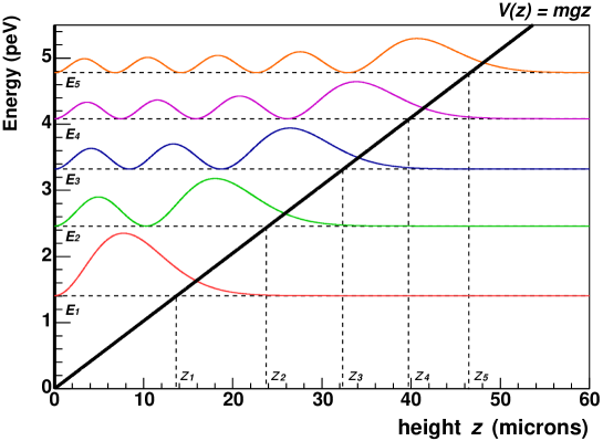
Figure 1: Probability distributions of gravitationally bound states of neutrons for the first five states[10]. Horizontal lines indicate eigenenegies $E_{n}$ and vertical lines show the classical turning points $z_{n}$ for each state.

This system is a suitable device with which to test the inverse square law of standard Newtonian gravity and to search for new gravity-like short-range interactions around these scales. The first limit to a non-Newtonian force with a Yukawa-type interaction potential using this microscopic system was reported in [11]. The limits for a CP-violating Yukawa-type potential were shown in [12, 13]. Several experimental schemes have been proposed to improve the sensitivity to such hypothetical new physics. One idea to achieve a better resolution on the measurement of the characteristic length is to utilize a convex reflection mirror to magnify the neutron distributions [14, 15]. In this review, we discuss an experiment using this scheme to precisely measure the UCN position-space wave functions, performed by the group of S. Komamiya of the University of Tokyo[16]. Experiments exploiting other ideas for measuring the energy scale, i.e. the energy differences between quantum states, are proposed by observing resonance transitions induced by a magnetic field[17, 18, 19, 20] and mechanical vibrations[21]. These projects are called GRANIT and qBounce, respectively. The first measurement of the resonance transition from the ground to the third state was reported by the group of H. Abele in [22]. For details of those projects, please see review papers [23] and [24] in this special issue.

Precision measurement and issues related to this analysis

The precision measurement with a convex magnification mirror[16] was performed using a UCN source provided at ILL(Institut Laue-Langevin)[25]. The velocity distribution was measured by a TOF method and is well characterized by a Gaussian distribution with mean of 9.4 m/s and standard deviation of 2.8 m/s. Figure 2(a) shows a schematic drawing of the experiment. The entire system was mounted on an anti-vibration table and magnetically shielded by a Permalloy sheet. The main components can be separated into three parts: a vertically thin collimating guide, a magnification mirror(rod), and a pixelated position sensitive detector. The layout of these components is shown in Fig. 2(b).

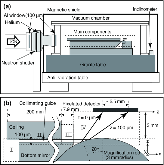
Figure 2: Schematic drawing of the precision measurement experiment using a convex magnification mirror[16]. (a) is an overview of the system and (b) shows the geometry of the main components.

Collimating guide

The guide settles gravitationally bound quantum states. To clearly distinguish each quantum state, which have energy differences of order of $\Delta E\sim 1~{}$peV, a resolving time of $\Delta t\sim\hbar/\Delta E\sim 1$ msec is required. Considering that the horizontal velocities of UCNs which we use are less than $15$ m/s, the collimating guide was designed to have a sufficient length (192 mm in our setup) to form each quantum states. The bottom mirror is made of polished glass with a roughness of $R_{a}$(arithmetic average) $=0.03~{}\mu$m. The ceiling scatterer is a Gd-Ti-Zr alloy (54/35/11) deposited on glass, with a Fermi potential tuned to be nearly zero, and a roughness of $R_{a}=0.4~{}\mu$m[30], which scatters out neutrons in the higher states. The guide selects lower states with appropriate populations to improve the contrast of the quantum spatial modulation. The neutron loss models for the scatterer or rough surface have been discussed in detail in [31, 32, 33], and they are still interesting issues not only for UCN guiding applications but also for storage experiments such as neutron EDM measurements. In the experiment reviewed in this paper, empirical models of the loss rates are adopted[16]. The loss rate by the scatterer, $\Gamma_{n}$, is assumed to be proportional to the probability of finding neutron in the roughness region, and is given by

$$\Gamma_{n}=\gamma\int_{h-2\delta}^{h}|\tilde{\psi_{n}}|^{2}dz~{},$$ (6)

where $\gamma$ is a scaling constant, estimated from data to be $9.5^{+0.7}_{-0.9}\times 10^{4}$ s^-1, $h$ is the height of the guide ($100~{}\mu$m), $\delta$ is the roughness of the scatterer ($0.4~{}\mu$m), and $\tilde{\psi_{n}}$ are deformed wave functions in the guide. Neutron losses at the bottom mirror due to absorption, non-specular reflection, up scattering and other processes are modeled empirically as

$$B_{n}=\beta\frac{g}{2\sqrt{2}}\sqrt{\frac{m}{\tilde{E_{n}}}}~{},$$ (7)

in which the loss rate is assumed to be proportional to the classical bouncing number per unit time, $g/2\tilde{v}_{z,n,max}$, where $\beta$ is a scaling constant (estimated to be $0.38^{+0.04}_{-0.03}$), $\tilde{v}_{z,n,max}\equiv\sqrt{2\tilde{E_{n}}/m}$ is the maximum vertical velocity of a neutron in the $n$th state, and $\tilde{E_{n}}$ is the eigenenergy of the deformed wave functions. The transmissivity of the guide for each state can be written as

$$\tilde{p_{n}}\propto\left<\exp[-\frac{l}{v_{x}}(\Gamma_{n}+B_{n})]\right>_{v_{x}}~{},$$ (8)

where $<...>_{v_{x}}$ indicate the average over the neutron horizontal velocities. By applying a diabatic transition from region II to III, the population distribution (a probability in the paper[16]) of neutrons for each state at the end of region III is estimated as in Fig. 3(a).

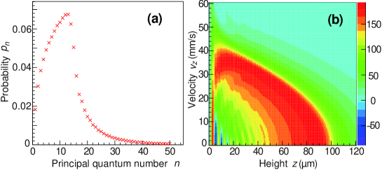
Figure 3: (a) is an estimated population distribution (probability distribution of the guide transmission) at the end of region III, and (b) shows the corresponding Wigner phase space distribution[16].

Magnification mirror

A Ni coated cylindrical rod is used as a magnifying convex mirror. Its radius is 3 mm and it is placed to have a grazing angle of 20 deg. for horizontally moving neutrons at the bottom floor level ($z=0$). Figure 4 shows the magnification power as a function of the height [10]. It gives about 20 times magnification around the lower region of $z\sim 20~{}\mu$m. Before depositing the Ni coating, the cylinder was polished at the Research Center for Ultra-Precision Science and Technology, Osaka University. The roughness of the rod after the depositing was measured to be $R_{a}=1.9$ nm, two orders of magnitude smaller than the neutron wavelength.

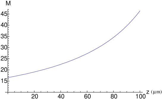
Figure 4: Magnification power $M$ of the cylindrical rod as a function of the height $z$[10]. It is about 20 times magnification around the lower region.

To calculate the detected position distribution on the detector surface, the wave function at the end of the bottom floor is re-expressed by the Wigner phase space distribution[37, 38],

$$W(z,p_{z})\equiv\frac{1}{2\pi\hbar}\int_{-\infty}^{\infty}\delta\eta~{}e^{-\frac{i}{\hbar}p_{z}\eta}<z+\frac{1}{2}\eta|\hat{\rho}|z-\frac{1}{2}\eta>~{},$$ (9)

where $p_{z}$ is the momentum and $\hat{\rho}$ is a density operator. The Wigner distribution is known as a phase space formulation of quantum mechanics, and is widely used for quantum optics, for example in the study of decoherence[39]. As an application to massive particles, one can find a paper which shows a phase-space tomography of the Wigner distribution for a coherent atomic beam in a double-slit experiment[40]. Figure 3(b) shows the Wigner distribution constructed from the estimated populations in our experiment[16]. The time evolution of the Wigner distribution is calculated by the evolution of the density operator described by the Liouville - von Neumann equation

$$\frac{\partial\hat{\rho}}{\partial t}=-\frac{i}{\hbar}[\hat{H},\hat{\rho}]~{},$$ (10)

where

$$\hat{H}=\frac{\hat{p_{z}^{2}}}{2m}+V(\hat{z})~{}.$$ (11)

By evaluating the kinetic part as

$$T=-\frac{p_{z}}{m}\frac{\partial}{\partial z}W(z,p_{z})~{},$$ (12)

and the potential part as

$$\sum_{l=0}^{\infty}U_{l}=\sum^{\infty}_{l=0}\frac{(-1)^{l}(\hbar/2)^{2l}}{(2l+1)!}\frac{d^{2l+1}V(z)}{dz^{2l+1}}\frac{\partial^{2l+1}}{\partial p_{z}^{2l+1}}W(z,p_{z})~{},$$ (13)

one can obtain the Quantum Liouville Equation for the Wigner distribution [41]

$$\left(\frac{\partial}{\partial t}+\frac{p_{z}}{m}\frac{\partial}{\partial z}-\frac{dV(z)}{dz}\frac{\partial}{\partial p_{z}}\right)W(z,p_{z})=\sum^{\infty}_{l=1}U_{l}~{}.$$ (14)

In the case of $V(z)=mgz$, the right hand side of the equation vanishes and it becomes the classical Liouville equation. Therefore, in region IV, one can treat the evolution of each phase point of the Wigner distribution as a classical path under gravity. Figure 5 shows the measured data and the best theoretical estimation using this model. The corresponding p-value is 0.715, and the experimental data support the quantum features described by the phase space formulation using the Wigner distribution[16].

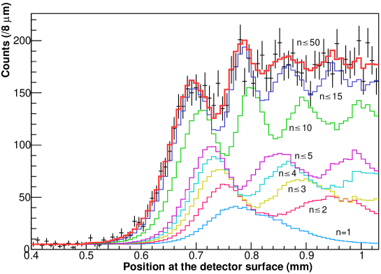
Figure 5: Black crosses show measured neutron position distribution[16]. Modulated distribution was clearly measured. The result shows good agreement with the quantum expectation calculated using phase space formalization by Wigner distribution (p-value is 0.715). The best estimated line is shown by a red solid curve and the other lines indicate contributions of each state to the distribution. For definitions of fitting parameters, best fit values, systematic uncertainties, and the other details, see [16].

Position sensitive detector for UCNs

A back-thinned CCD (HAMAMATSU S7030-1008) with thin Ti-¹⁰B-Ti layers is used for the position sensitive detector in the experiment[16]. Its pixel size is $24~{}\mu$m $\times$ $24~{}\mu$m and the thickness of the active volume is about $20~{}\mu$m. The ¹⁰B layer converts neutrons into charged particles by the nuclear reaction ¹⁰B(n,$\alpha$)⁷Li. The secondary particles are emitted in a nearly back-to-back configuration. One of them deposits its kinetic energy in the active area and creates a charge cluster, which typically spreads into nine pixels. The weighted center of the charge cluster is a good estimation of the incident neutron position. The thickness of the layers are 20 nm and 200 nm for Ti and ¹⁰B, respectively, and they are formed by evaporating directly on the CCD surface. The spatial resolution is measured to be $3.35\pm 0.09~{}\mu$m by evaluating the line spread function (LSF) (see Fig. 6) using very cold neutron beams at ILL[10]. For the detail of the evaluation scheme, see [15, 42]. A neutron converter of ⁶Li using ⁶Li(n,$\alpha$)³H reaction was also investigated. It is concluded that the use of ¹⁰B gives better spatial resolution[42].

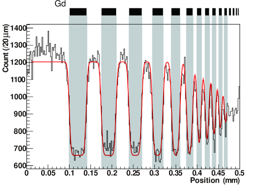
Figure 6: Fitting results of a Gd shadow pattern[10]. Spatial resolution is measured to be $3.35\pm 0.09~{}\mu$m by evaluating these line spread functions. For details of evaluation method, see [15, 42].

Other detectors using a silicon pixel device, Timepix[43], with ⁶LiF and ¹⁰B converter were studied in [44]. Its pixel pitch is $55~{}\mu$m $\times$ $55~{}\mu$m and the thickness of its silicon layer is about $300~{}\mu$m. The spatial resolution for the ⁶LiF converter was evaluated by LSF to be $2.3~{}\mu$m, corresponding to about $5.3~{}\mu$m in FWHM of the point spread function (PSF). The performance of the ¹⁰B converter is estimated by Monte-Carlo simulations to be better than $3~{}\mu$m in FWHM of the PSF.

Another detector concept of Uranium coated plastic nuclear tracker (CR39) [9] was used in several experiments[8, 34, 35, 36, 45]. Usually two fission fragments are emitted from a thin ²³⁵U coating, and one of the daughter nuclei makes a track of defects in the CR39. By chemical etching, the diameter of track points is increased up to 1 $\mu$m, allowing us to scan these vertexes using an optical microscope. Position resolution is around $1~{}\mu$m[9]. By carefully analyzing the vertex shape, the spatial resolution can be improved to $0.7~{}\mu$m[45].

Summary

The quantum system of a gravitationally bound neutron is one of the most suitable tools to investigate gravity or gravity-like hypothetical interactions around the scale of $10~{}\mu$m in length or 1 peV in energy. After establishing this research field by the pioneering work in observation of the quantum state[6], experimental schemes for precision measurements of these characteristic scales have developed rapidly, and nowadays, one can establish limits for parameter spaces of new physics experimentally[11, 12, 13, 26]. Furthermore one can start discussing a phase space formulation of quantum physics for the gravitationally bound quantum state [16]. An experiment for a possible test of phase space formalization using spatial interference is under preparation.

References

- [1] R. Colella, A. W. Overhauser, and S. A Werner, Phys. Rev. Lett. 34, 1472 (1975)
- [2] J. J. Sakurai, Phys. Rev. D 21, 2993 (1980)
- [3] J. L. Staudenmann et al., Phys. Rev. A 21, 1419 (1980)
- [4] S. A. Werner et al., Physica B 151, 22 (1988)
- [5] K. C. Littrell, B. E. Allman, and S. A. Werner, Phys. Rev. A 56, 1767 (1997)
- [6] V. V. Nesvizhevsky et al., Nature 415, 297 (2002)
- [7] V. V. Nesvizhevsky et al., Phys. Rev. D 67, 102002 (2003)
- [8] V. V. Nesvizhevsky et al., Eur. Phys. J. C 40, 479 (2005)
- [9] V. V. Nesvizhevsky et al., Nucl. Instrum. Meth. A 440, 754 (2000)
- [10] G. Ichikawa, PhD. Dissertation, The University of Tokyo (2013)
- [11] V. V. Nesvizhevsky and K. V. Protasov, Class. Quantum Grav. 21, 4557 (2004)
- [12] S. Baeßler it et al., Phys. Rev. D 75, 075006 (2007)
- [13] S. Baeßler it et al., Nucl. Instrum. Meth. A 611, 149 (2009)
- [14] V. V. Nesvizhevsky, Preprint ILL 96NE14T (1994)
- [15] T. Sanuki et al., Nucl. Instrum. Meth. A 600, 657 (2009)
- [16] G. Ichikawa et al., Phys. Rev. Lett. 112, 071101 (2014)
- [17] P. Schmidt-Wellenburg et al., Nucl. Instrum. Meth. A 611, 267 (2009)
- [18] M. Kreuz et al., Nucl. Instrum. Meth. A 611, 326 (2009)
- [19] S. Baeßler et al. (GRANIT Collaboration), C. R. Physique 12, 707 (2011)
- [20] V. V. Nesvizhevsky (GRANIT Collaboration), Mod. Phys. Lett. A 27, 1230006 (2012)
- [21] H. Abele et al., Phys. Rev. D 81, 065019 (2010)
- [22] T. Jenke et al., Nature Phys. 7, 468 (2011)
- [23] D. Roulier et al., Adv. High En. Phys. this issue (2014)
- [24] G. Cronenberg et al., Adv. High En. Phys. this issue (2014)
- [25] A. Steyeri et al., Phys. Lett. A 116, 347 (1986)
- [26] T. Jenke et al., Phys. Rev. Lett. 112, 151105 (2014)
- [27] J. Khoury and A. Weltman, Phys. Rev. Lett. 93, 171104 (2004)
- [28] D. F. Mota and D. J. A. Shaw, Phys. Rev. Lett. 97, 151102 (2006)
- [29] J. Khoury, Class. Quantum Grav. 30, 214004 (2013)
- [30] Y. Kamiya et al., KURRI Progress Report CO1-1 (2008)
- [31] A. E. Meyerovich and V. V. Nesvizhevsky, Phys. Rev. A 73, 063616 (2006)
- [32] A. Yu. Voronin et al., Phys. Rev. D 73, 044029 (2006)
- [33] A. Westphal et al., Eur. Phys. J. C 51, 367 (2007)
- [34] V. V. Nesvizhevsky et al., ILL Annual Report (2004)
- [35] H. Abele et al., Nucl. Phys. A 827, 593c (2009)
- [36] T. Jenke et al., Nucl. Instrum. Meth. A 611, 318 (2009)
- [37] E. Wigner, Phys. Rev 40, 749 (1932)
- [38] M. Hillery et al., Phys. Rep. 106, 121 (1984)
- [39] L. Mandel and E. Wolf, Optical Coherence and Quantum Optics (Cambridge University Press 1995)
- [40] Ch. Kurtsiefer, T Pfau, and J. Mlynek, Nature 386, 150 (1997)
- [41] W. P. Schleich, Quantum Optics in Phase Space (Wiley-VCH 2001)
- [42] S. Kawasaki et al., Nucl. Instrum. Meth. A 615, 42 (2010)
- [43] X. Llopart et al., Nucl. Instrum. Meth. A 581, 485 (2007)
- [44] J. Jakubek et al., Nucl. Instrum. Meth. A 600, 651 (2009)
- [45] T. Jenke et al., Nucl. Instrum. Meth. A 732, 1 (2013)