On the polar cap cascade pair multiplicity of young pulsars

Abstract

We study the efficiency of pair production in polar caps of young pulsars under a variety of conditions to estimate the maximum possible multiplicity of pair plasma in pulsar magnetospheres. We develop a semi-analytic model for calculation of cascade multiplicity which allows efficient exploration of the parameter space and corroborate it with direct numerical simulations. Pair creation processes are considered separately from particle acceleration in order to assess different factors affecting cascade efficiency, with acceleration of primary particles described by recent self-consistent non-stationary model of pair cascades. We argue that the most efficient cascades operate in the curvature radiation/synchrotron regime, the maximum multiplicity of pair plasma in pulsar magnetospheres is $\sim\mbox{few}\times 10^{5}$. The multiplicity of pair plasma in magnetospheres of young energetic pulsars weakly depends on the strength of the magnetic field and the radius of curvature of magnetic field lines and has a stronger dependence on pulsar inclination angle. This result questions assumptions about very high pair plasma multiplicity in theories of pulsar wind nebulae.

1. Introduction

The idea that production of electron-positron pairs in magnetospheres of rotation-powered pulsars is intimately connected with their activity had been proposed by Sturrock (1971) only a few years after the discovery of pulsars (Hewish et al., 1968). Since then it has become an integral part of the standard pulsar model and today, there is little doubt that an active rotationally powered pulsar produces electron-positron plasma. Although the pulsar emission mechanism(s) is still not yet identified, there is strong empirical evidence that pulsars stop emitting radio waves when pair formation ceases – the threshold for pair formation roughly corresponds to the “death line” in pulsar parameter space, what was already noted by Sturrock (1971). Furthermore, the narrow peaks in many pulsar high-energy light curves (Abdo et al., 2010) require pervasive screening of the whole magnetosphere by pair plasma, except in narrow accelerator gaps (e.g. Watters et al., 2009; Pierbattista et al., 2015). Understanding pair plasma generation in pulsar magnetospheres is therefore of crucial importance for developing pulsar emission models.

In the standard pulsar model, initially proposed by Goldreich & Julian (1969) and Sturrock (1971), the magnetosphere is filled with dense pair plasma which screens the accelerating electric field everywhere except some small zones which are responsible for particle acceleration and emission. Pair plasma is primarily created via conversion of $\gamma$ rays in the strong magnetic field near the polar caps (PCs). Pair production in the PCs is a “cornerstone” of the standard model – without dense plasma produced at the PCs, at the base of open magnetic field lines, the magnetosphere would have large volumes with unscreened electric field, as pair creation in e.g. outer gaps (Cheng et al., 1976) cannot screen the electric field over the rest of the magnetosphere.

Charge starvation (Arons & Scharlemann, 1979) or vacuum gaps (Ruderman & Sutherland, 1975) at the polar cap, when the number density of charged particles is not enough to screen the electric field, leads to formation of accelerating zone(s). Some charged particles enter this zone, are accelerated to very high energies and emit gamma-rays which are absorbed in the ultrastrong magnetic field, creating electron-positron pairs. The pairs, being relativistic, can also emit pair producing photons and so the avalanche develops until photons emitted by the last generation of pairs can no longer produce pairs and escape the magnetosphere.

The pair plasma created by pulsars flows out of the magnetosphere along open magnetic field lines and provides the radiating particles for the surrounding Pulsar Wind Nebulae (PWNe). Models of PWNe depend (at least) on the density of the plasma, what produces the observed synchrotron and inverse Compton emission. Estimates of the pair multiplicity (the number of pairs produced by each primary accelerated particle) needed to account for the emission from the Crab pulsar wind nebula (PWN) range from about $10^{5}-10^{6}$ (de Jager et al., 1996) up to $10^{7}$ (e.g. Bucciantini et al., 2011); for the Vela PWN the multiplicity is estimated to be about $10^{5}$ (de Jager, 2007). PWNe therefore give the most compelling evidence for pair production and pair cascades in at least young energetic pulsar magnetospheres.

Although PWNe are observed only around young pulsars ($<$ a few times $10^{4}$ yrs), evidence for pairs, at least for high plasma densities larger than those provided by primary particles, can also be found in older pulsars. Synchrotron absorption models for the eclipse in the double pulsar system PSR J0737-3039 (Arons et al., 2005; Lyutikov, 2004) require a pair multiplicity of around $10^{6}$ for the recycled 22 ms pulsar in that system.

The cascade process in pulsar polar caps has been the subject of extensive numerical as well as analytical studies (e.g. Daugherty & Harding, 1982; Gurevich & Istomin, 1985; Zhang & Harding, 2000; Hibschman & Arons, 2001a, b; Medin & Lai, 2010). The pair plasma multiplicity obtained in these studies was significantly lower than estimates of pair plasma multiplicity in PWNe, as it did not exceed $\sim$few$\times 10^{4}$. Most of those works considered pair creation together with the particle acceleration which makes these analyses dependent on the acceleration model considered. These studies also assumed steady, time-independent acceleration of the primary particles. However, recent studies by Timokhin (2010); Timokhin & Arons (2013) have found that pulsar polar cap pair cascades are not time-steady in the general case of arbitrary current, particularly those required by global magnetosphere models (e.g Contopoulos et al., 1999; Timokhin, 2006; Spitkovsky, 2006; Kalapotharakos & Contopoulos, 2009).

In this paper we study the question of what is the maximum pair multiplicity achievable in pulsar polar cap cascades and under which circumstances is it achieved. In contrast to previous pair cascade studies, we take a multistep approach. We consider the physical processes in pair cascades and particle acceleration models separately in order to clearly set apart different factors influencing the efficiency of pair cascades. We first assess how each of the microscopic processes affects the final multiplicity and the pulsar parameter ranges that result in the largest possible pair multiplicity. Then, we employ the most recent model of non steady-state particle acceleration in pulsar polar caps and derive a simple analytical estimate for the maximum energy of particles accelerated in a non-stationary cascade. One on the most important results of our study is a strong upper limit on pair plasma multiplicity in pulsars.

We limit ourselves to the case of cascades at the polar caps of young pulsars as from previous theoretical studies of polar cap cascades, such pulsars are expected to be the most efficient pair producers. We rely on results of previous cascade studies in our choice of the specific cascade process, namely cascades initiated by curvature radiation of primary particles.

The plan of the paper is as follows. In § 2 we briefly discuss the efficiency of cascades in general and give an overview of the most efficient cascade process in pulsar polar caps. In subsequent sections we consider in detail all physical processes in such cascades. §§3–7, the largest part of this paper, are devoted to development of a simple semi-analytical model for estimation of pair production efficiency in polar caps of young pulsars. This model allows efficient exploration of pulsar parameter space and helps to clarify the main factors affecting cascade multiplicity. Then, in §8 we use direct numerical simulations of PC cascades in a Crab-like pulsar to show that predictions of our semi-analytical model are indeed correct. We discuss uncertainties of current pulsar models in § 10 and summarize and discuss our findings and their implications in the Discussion.

2. Physics of polar cap cascades: an overview

An electron-positron cascade can be thought of as a process of splitting the energy of primary particles into the energies of secondary particles. The maximum multiplicity, the number of secondary particles for each primary particle, of an ideal cascade initiated by a single primary particle with energy $\epsilon_{p}$ would be

$$\kappa_{\textrm{\scriptsize{max}}}\simeq{}2\,\frac{\epsilon_{p}}{\epsilon_{\gamma,\,\textrm{\scriptsize{esc}}}}\,.$$ (1)

where $\epsilon_{\gamma,\,\textrm{\scriptsize{esc}}}$ is the maximum energy of photons escaping from the cascade (or the minimum energy of pair producing photons). Not all of the primary particle energy goes into pair producing photons, and pairs created in the cascade do not radiate all of their energy into the next generation of pair producing photons. Hence, $\kappa_{\textrm{\scriptsize{max}}}$ is only the theoretical upper limit on the multiplicity of a real cascade. The total pair yield of the cascade is a combination of four factors: (a) number of primary particles, (b) initial energy of primary particle – the higher the energy the more pairs can be produced, (c) threshold for pair formation – the lower the threshold the higher the multiplicity, (d) efficiency of splitting the energy of primary particles into pairs – the higher the fraction of particle energy going into pair creating photons, as opposed to the final kinetic energy of the particles and photons below the pair formation threshold, the higher the multiplicity.

In young, fast rotating pulsars, the electric field in the polar cap acceleration zones is strong and primary particles can be accelerated up to very high Lorentz factors, $\gamma\gtrsim{}10^{7}$. At these energies the most effective radiation process is curvature radiation (CR). CR efficiency grows rapidly with the particle energy and for young pulsars becomes the dominant emission mechanism for primary particles. For secondary particles, which are substantially less energetic than the primary ones, the primary way to create pair producing photons is via synchrotron radiation. In § 9 we argue that although another possible emission mechanism for secondary particles – Resonant Inverse Compton Scattering (RICS) of soft X-ray photons emitted by the NS – can generate pair producing photons in pulsars with magnetic field $\gtrsim\mbox{$3\times 10^{11}$}$ G, that channel never becomes the dominant one for pair production in young pulsars, at best resulting in pair multiplicity comparable to the one of the synchrotron channel. Hence, in young pulsars which are expected to have the highest multiplicity pair plasmas, the polar cap cascades should operate primarily in the CR-synchrotron regime – all known studies of cascades in pulsar polar cap agree on this point. In this paper we study in detail CR-synchrotron cascades. The resulting multiplicities will be good estimates for a wide range of pulsar parameters, however, as we consider only synchrotron radiation of secondary particles, for pulsars with magnetic field $\gtrsim\mbox{$3\times 10^{12}$}$ G our analysis might underestimate the cascade multiplicity by a factor of $\sim 2$, see § 9.

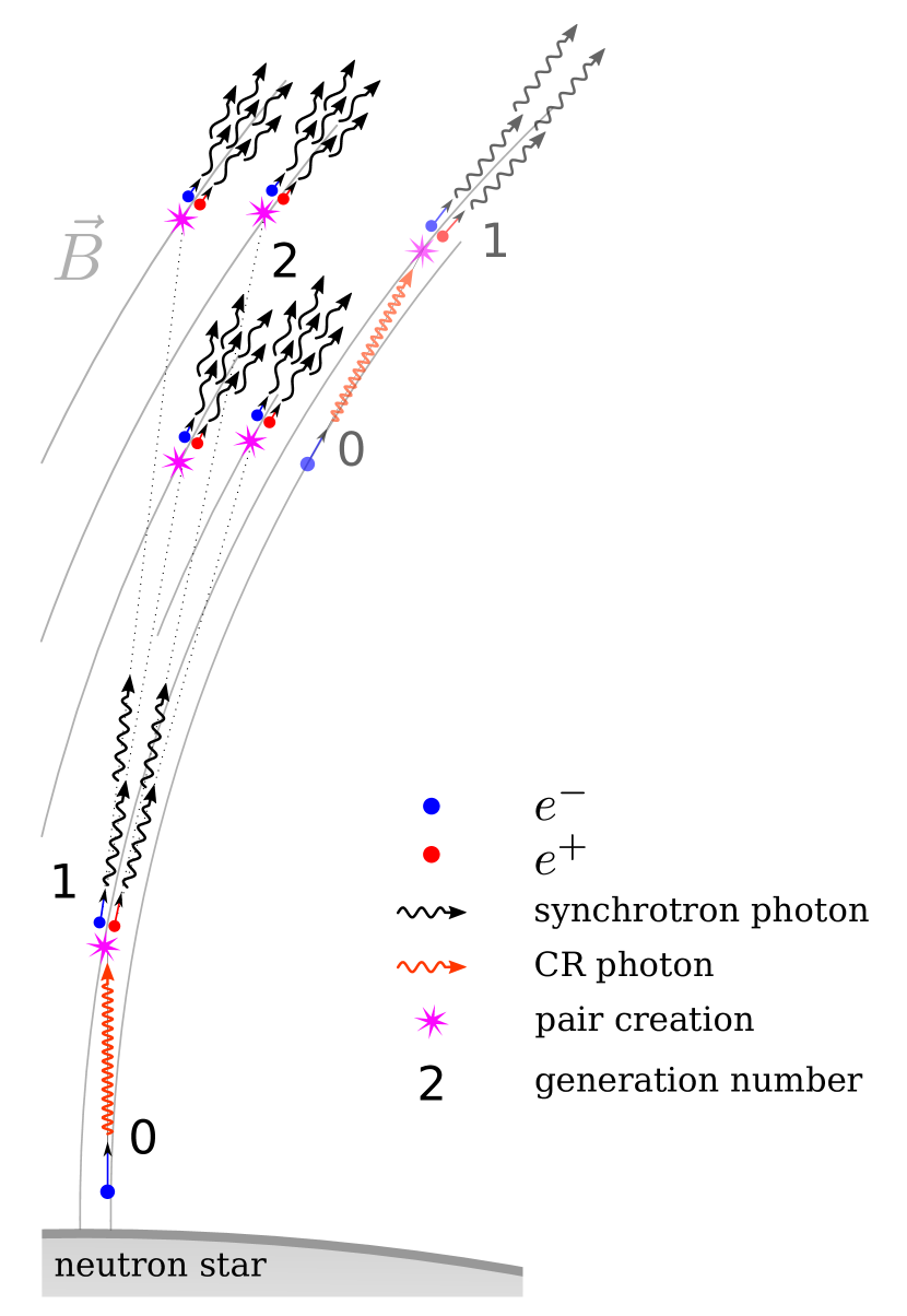
Figure 1.— Schematic representation of electron-positron cascade in the polar cap of a young pulsar, see text for description.

Fig. 1 gives a schematic overview of electron-positron cascade development in polar cap regions of young pulsars. Shown are the first two generations in a cascade initiated by a primary electron. Primary electrons emit CR photons (almost) tangent to the magnetic field lines; primary electrons and CR photons are generation 0 particles in our notation. Magnetic field lines are curved and the angle between the photon momentum and the magnetic field grows as the photon propagates further from the emission point. When this angle becomes large enough, photons are absorbed and each photon creates an electron-positron pair – generation 1 electron and positron. The pair momentum is directed along the momentum of the parent photon and at the moment of creation, the particles have non-zero momentum perpendicular to the magnetic field. They radiate this perpendicular momentum almost instantaneously via synchrotron radiation and then move along magnetic field lines. Although these secondary particles are relativistic, their energy is much lower than that of the primary electron and their curvature photons cannot create pairs. After the emission of synchrotron photons, secondary particles (generation 1 and higher) no longer contribute to cascade development. Generation 1 photons (synchrotron photons produced by the generation 1 particles) are also emitted (almost) tangent to the magnetic field line – as the secondary particles are relativistic – and propagate some distance before acquiring the necessary angle to the magnetic field and creating generation 2 pairs. These pairs in their turn radiate their perpendicular momentum via synchrotron radiation, emitting generation 2 photons. The cascade initiated by a single CR photon stops at a generation where the energy of synchrotron photons falls below $\epsilon_{\gamma,\,\textrm{\scriptsize{esc}}}$.

Only primary particles emit pair producing photons as they move along the field lines; all secondary particles emit pair producing photons just after their creation. The cascade development can be thus divided into two parts: (i) primary particles emit CR photons as they move along magnetic field lines and (ii) each CR photon gives rise to a synchrotron cascade, when synchrotron photons create a successive generation of pairs which emit the next generation synchrotron photons at the moment of creation. This division goes between generation 0 and all subsequent cascade generations.

In the following sections we analyze all four factors regulating the yield of CR-synchrotron cascades listed at the beginning of this section (in reverse order, from d to a). In §§3–7 we develop a simple semi-analytical models for calculation of multiplicity of strong polar caps cascades initiated by a primary electron which we then compare with detailed numerical computation described in §8. We start with gamma-ray absorption in a strong magnetic field in §3; then we discuss the efficiency of the synchrotron cascade in §4. Curvature radiation is considered in §5 and in §5.3 we discuss the multiplicity of a CR-synchrotron cascade initiated by a single particle of given energy. This covers items c and d from the list of factors affecting cascades efficiency. In §6 we address item b from the list - energy of primary particles initiating the cascade. §§7 and 8 are devoted to the total multiplicity of a CR-synchrotron cascade when particle acceleration is taken into account - in §7 we present results for cascade multiplicities from a semi-analytical model and in §8 we present results of detailed numerical simulations of cascades in a Crab-like pulsar. In §9 we discuss the role of RICS in polar caps cascades and argue that considering only CR-synchrotron cascades gives us an adequate estimate of the pair multiplicity in young pulsars. Finally, in §10, we address item a – the mean flux of primary particles and the total yield of a CR-synchrotron cascade in an energetic pulsar. We argue that this is the most important factor regulating pair yield in energetic pulsars. Despite the uncertainty in determining the mean flux of primary particles, we can set a rather strict upper limit on pair multiplicity in pulsars.

3. Photon absorption in the magnetic field

3.1. Opacity for $\gamma-B$ pair production

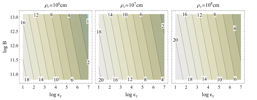
Figure 2.— Contour plot of $1/\chi_{a}$ as a function of the logarithms of the magnetic field strength $B$ in Gauss, and photon energy $\epsilon_{\gamma}$ normalized to the electron rest energy, for three values of the radius of curvature of magnetic field lines $\rho_{\textrm{\scriptsize{c}}}=10^{6},10^{7},10^{8}\mbox{cm}$. $1\chi_{a}$ values shown on this plot are calculated from eq. (7) and are not corrected for the kinematic threshold (see text).

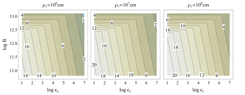
Figure 3.— Contour plot of $1/\chi_{a}$ corrected for kinematic threshold according to eq. (9). These values of $1/\chi_{a}$ are used in all calculations within semi-analytic model. Notations are the same as in Fig. 2.

The opacity for single photon pair production in strong magnetic field is (Erber, 1966)

$$\alpha_{B}(\epsilon_{\gamma},\psi)=0.23\,\frac{\alpha_{f}}{\lambdabar{}_{\textrm{\scriptsize{{c}}}}}\>b\,\sin\psi\,\exp\left(-\frac{4}{3\chi}\right)$$ (2)

where $b\equiv{}B/B_{q}$ is the local magnetic field strength $B$ normalized to the critical quantum magnetic field $B_{q}=e/\alpha_{f}\lambdabar{}_{\textrm{\scriptsize{{c}}}}^{2}=\mbox{$4.41\times 10^{13}$}$ G, $\psi$ is the angle between the photon momentum and the local magnetic field, $\alpha_{f}=e^{2}/\hbar{}c\approx{}1/137$ is the fine structure constant, and $\lambdabar{}_{\textrm{\scriptsize{{c}}}}=\hbar/mc=\mbox{$3.86\times 10^{-11}$}$ cm is the reduced Compton wavelength. The parameter $\chi$ is defined as

$$\chi\equiv\frac{1}{2}\,\epsilon_{\gamma}b\,\sin\psi\,,$$ (3)

where $\epsilon_{\gamma}$ is the photon energy in units of $m_{e}c^{2}$. For convenience from here on, all particle and photon energies will be quoted in terms of $m_{e}c^{2}$. The optical depths for pair creation by a high energy photon in a strong magnetic field after propagating distance $l$ is

$$\tau(\epsilon_{\gamma},l)=\int_{0}^{l}\alpha_{B}(\epsilon_{\gamma},\psi(x))\,dx\,,$$ (4)

where integration is along the photon’s trajectory.

Expression (2) is accurate if the magnetic field is small compared to the critical field $B_{q}$, $b<0.2$ suffices, and if $\epsilon_{\gamma}\sin\psi>2$ so that the created pair is in a high Landau level; pair production into low Landau levels and for higher magnetic fields has been discussed in Daugherty & Harding (1983) and Harding et al. (1997). For most pulsars, the magnetic field in polar cap regions is smaller that $B_{q}/3$. In this paper we study cascades in pulsars with “normal” magnetic fields and so we neglect high-field effects.

Expression (2) becomes inaccurate when pairs are created at low Landau levels, near the pair formation threshold, it overestimates the opacity and even formally allows pair formation below the kinematic threshold $\epsilon_{\gamma}\sin\psi=2$. However, pairs created at low Landau levels will not give rise to strong cascades, as their perpendicular energy will be too low to emit pair-producing synchrotron photons. Hence, for the case of strong cascades, accurate treatment of pair formation near the kinematic threshold is not necessary. Throughout this paper we use Erber’s approximation (2) in all our analytical calculations but introduce a cut off at the kinematic threshold $\epsilon_{\gamma}\sin\psi=2$ as described at the end of this section, thus taking into account the cessation of pair formation below the the kinematic threshold.

If the mean free path (mfp) of a pair-producing photon $l_{\gamma}$ is comparable to or larger than the characteristic scale of the magnetic field variation $L_{B}$, this photon will not initiate a strong cascade with the same emission processes by which it was produced. The reason for this is as follows. The opacity for $\gamma{}B$ pair production exponentially depends on the magnetic field strength and photon energy via $\chi$. The energy of the next generation photon will be smaller than that of the primary one, and, because the primary photon has already traveled the distance over which the magnetic field has substantially declined, the magnetic field along the next generation photon’s trajectory will be substantially weaker than that along the primary photon’s trajectory. The next generation photon’s mfp will be much larger than than that of the primary photon, and, even if this secondary photon will be absorbed, it will be the last cascade generation. Hence, in a strong cascade, for all but the last generation photons, $l_{\gamma}\ll{}L_{B}$. A reasonable estimate for $L_{B}$ would be the distance of the order of the NS radius $R_{\textrm{\scriptsize{{ns}}}}$ as any global NS magnetic field decays with the distance as $(r/R_{\textrm{\scriptsize{{ns}}}})^{-\delta}$, $\delta\geq 3$. Very localized, sun spot like magnetic fields, are in our opinion of no importance for the general pulsar case as the probability of such a “spot” to lie at the polar cap should be rather low, i.e. most pulsars should be able to produce plasma in a more or less regular magnetic field. A dipole field, $\delta=3$, is often considered as a reasonable assumption for a general pulsar model. Pure dipole field, however, seems to be a too idealized approximation, as even if the NS field is a pure dipole, it will be slightly disturbed by the currents flowing in the magnetosphere. In general, near dipole magnetic fields with different curvatures of magnetic field lines should be examined in cascade models.

We consider strong cascades with large multiplicities, where, as argued above, photons propagate distances much shorter than the characteristic scale of the magnetic field variation, so we assume that in the region where most of the pairs are produced the magnetic field is constant. The radius of curvature of magnetic field lines $\rho_{\textrm{\scriptsize{c}}}$ is not smaller than $L_{B}$, and as $l_{\gamma}\ll{}L_{B}$ the angle $\psi$ is always small, the approximation $\sin\psi\approx\psi$ is very accurate. For photons emitted tangent to the magnetic field line, $dx=\rho_{\textrm{\scriptsize{c}}}d\psi$. In our approximation both $b$ and $\rho_{\textrm{\scriptsize{c}}}$ are constants. From eq. (3) we have $\psi=2\chi/\epsilon_{\gamma}{}b$, and substituting it into eq. (4) we can express the optical depth $\tau$ to pair production as an integral over $\chi$

$$\tau(\epsilon_{\gamma},l)=A_{\tau}\,\frac{\rho_{\textrm{\scriptsize{c}}}}{\epsilon_{\gamma}^{2}b}\;\int_{0}^{\chi(\epsilon_{\gamma},\psi(l))}\chi\exp\left(-\frac{4}{3\chi}\right)\,d\chi\,,$$ (5)

where $A_{\tau}\equiv{}0.92\alpha_{f}/\lambdabar{}_{\textrm{\scriptsize{{c}}}}\approx\mbox{$1.74\times 10^{8}$}\;\mbox{cm}^{-1}$.

Integrating eq. (5) over $\chi$ by parts two times we can get an expression for $\tau$ in terms of elementary functions and the exponential integral function Ei:

$$\tau(\chi) = A_{\tau}\,\frac{\rho_{\textrm{\scriptsize{c}}}}{\epsilon_{\gamma}^{2}b}\times$$ (6)

$$\left[\frac{\chi^{2}}{2}\left(1-\frac{4}{3\chi}\right)e^{-\frac{4}{3\chi}}-\frac{8}{9}\,\mbox{Ei}\left(-\frac{4}{3\chi}\right)\right]\,.$$

$\mbox{Ei}(z)$ is a widely used special function, defined as $\mbox{Ei}(z)=-\int_{-z}^{\infty}\exp(-t)/t\,dt$. There are efficient numerical algorithms for its calculation implemented in many numerical libraries and scientific software tools; using eq. (6) for calculation of the optical depths will result in much more efficient numerical codes than direct integration of eq. (5).

As the optical depth to pair formation grows exponentially with $\chi$ (and distance), for analytical estimates it is reasonable to assume that all photons are absorbed when they have traveled the distance $l_{\gamma}$ such that $\tau(l_{\gamma})=1$. We denote the value of $\chi$ when the optical depth reaches 1 as $\chi_{a}:$

$$\chi_{a}:\tau(\chi_{a})=1\,.$$ (7)

In all our computations we will use $\chi_{a}$ as the value of the parameter $\chi$ at the point of the photon’s absorption. $\chi_{a}$ is a solution of the non-linear equation (7) with $\tau$ given by eq. (6). Because of the exponential dependence of $\tau$ on $1/\chi$ it is to be expected that $1/\chi_{a}$ should have a close to linear dependence on logarithms of $\epsilon_{\gamma}$, $b$, and $\rho_{\textrm{\scriptsize{c}}}$. We solved equation (7) numerically for different values of $\epsilon_{\gamma}$, $b$, and $\rho_{\textrm{\scriptsize{c}}}$ and, indeed, the inverse quantity $1/\chi_{a}$ depends almost linearly on $\log\epsilon_{\gamma}$, $\log{}b$, and $\log\rho_{\textrm{\scriptsize{c}}}$ in a wide range of these parameters. Making a modest size table of $1/\chi_{a}$ values one can later use piecewise interpolation to find a particular value of $\chi_{a}$ quite accurately.

In Fig. 2 we plot contours of $1/\chi_{a}$ as functions of $\log(\epsilon_{\gamma})$ and $\log(B)$ for three different values for the radius of curvature of the magnetic field lines. We want to point out that $1/\chi_{a}$ differs from the value $1/\chi_{a}=15$ used by Ruderman & Sutherland (1975), especially for higher energy photons. Although this difference is only a factor of a few, as we will point out later, the cascade efficiency in each generation depends on the corresponding value of $\chi_{a}$, and in a strong cascade with several generations, the estimate for the final multiplicity will be substantially affected by the value of $\chi_{a}$.

Erber’s expression is not applicable for pairs produced at low Landau levels as it overestimates the opacity and, formally, solutions for $\chi_{a}$ obtained from eq. (7) allows pair creation even for $\epsilon_{\gamma}\sin\psi<2$. In our analytical treatment we introduce a limit on $\chi_{a}$ to correct for the kinematic threshold. For photons above kinematic threshold from eq. (3) it follows that

$$\chi_{a}>b\,,$$ (8)

In all our analytical calculation we get $\tilde{\chi}_{\textrm{\scriptsize{a}}}$ from eq. (7) and then use the maximum value of $\tilde{\chi}_{\textrm{\scriptsize{a}}}$ and $b$:

$$\chi_{a}=\max\left(\tilde{\chi}_{\textrm{\scriptsize{a}}},\;b\right)\,.$$ (9)

In Fig. 3 we plot contours of $1/\chi_{a}$ which incorporate corrections to $\chi_{a}$ due to the kinematic threshold according to eq. (9). It is clear from the plot that this correction affects only cases with high magnetic field and low particle energies.

3.2. Energy of escaping photons

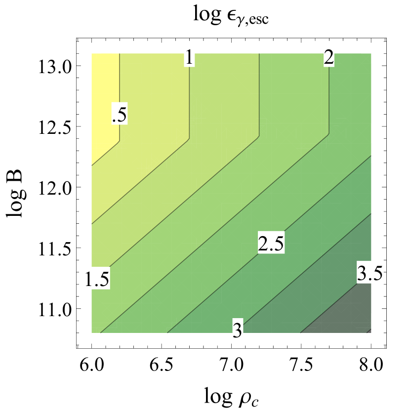
Figure 4.— Energy of escaping photons: contours of $\log{\epsilon_{\gamma,\,\textrm{\scriptsize{esc}}}}$ as a function of logarithms of the radius of curvature of magnetic field lines $\rho_{\textrm{\scriptsize{c}}}$ in cm and magnetic field strength $B$ in Gauss for $s_{\textrm{\scriptsize{esc}}}=1$.

As discussed above, photons escaping the cascade are those whose mfp $l_{\gamma}$ is larger than the distance of significant magnetic field attenuation $L_{B}$. The formal criteria we use for calculating the energy of escaping photons $\epsilon_{\gamma,\,\textrm{\scriptsize{esc}}}$ is $l_{\gamma}(\epsilon_{\gamma,\,\textrm{\scriptsize{esc}}})=s_{\textrm{\scriptsize{esc}}}R_{\textrm{\scriptsize{{ns}}}}$; $s_{\textrm{\scriptsize{esc}}}$ is a dimensionless parameter quantifying the escaping distance in units of $R_{\textrm{\scriptsize{{ns}}}}$. The photon mfp is $l_{\gamma}{}=\rho_{\textrm{\scriptsize{c}}}\psi_{a}$ and expressing the angle between the photon momentum and the magnetic field at the point of absorption $\psi_{a}$ through $\chi_{a}$ we get a (non-linear) equation for $\epsilon_{\gamma,\,\textrm{\scriptsize{esc}}}$

$$\epsilon_{\gamma,\,\textrm{\scriptsize{esc}}}=2\,\frac{\rho_{\textrm{\scriptsize{c}}}}{s_{\textrm{\scriptsize{esc}}}R_{\textrm{\scriptsize{{ns}}}}}\frac{\chi_{a}(\epsilon_{\gamma,\,\textrm{\scriptsize{esc}}},b,\rho_{\textrm{\scriptsize{c}}})}{b}\,.$$ (10)

The non-linearity in this equation is due to dependence of $\chi_{a}$ on $\epsilon_{\gamma,\,\textrm{\scriptsize{esc}}}$, $b$, and $\rho_{\textrm{\scriptsize{c}}}$. Using an interpolation table for $1/\chi_{a}$ this equation is very easy to solve numerically for all reasonable values of physical parameters involved.

In Fig. 4 we plot energy of escaping photons, $\log{\epsilon_{\gamma,\,\textrm{\scriptsize{esc}}}}$ as a function of the radius of curvature of magnetic field lines $\rho_{\textrm{\scriptsize{c}}}$ and magnetic field strength $B$ for $s_{\textrm{\scriptsize{esc}}}=1$. For smaller values of $s_{\textrm{\scriptsize{esc}}}$ the whole plot would move to the left. This figure shows (an obvious) trend that for higher magnetic field and smaller radii of curvature, the energy of escaping photons is lower, which allows for more cascade generations and larger multiplicity. The break in contour lines around $\log{B}\simeq 12.4$ is due to the kinematic threshold.

For a given geometry of the magnetic field a more accurate analytical expression for the energy of escaping photons can be derived using an exact expression for $\psi$ along photon’s travel path by expanding the integral in eq. (4) around its upper endpoint, as was done by Hibschman & Arons (2001b). However here we try to explore different possible magnetic field configuration – exploring parameter space in $\rho_{\textrm{\scriptsize{c}}}$ – and our simple estimate is accurate to a factor of a few.

4. Synchrotron Cascade

In this section we discuss the synchrotron cascade, where most of the electron-positron pairs are created. The synchrotron cascade is the part of the whole cascade that is initiated by generation 0 photons. In the synchrotron cascade each generation’s primary photon is divided into many (lower energy) next generation’s pair-producing photons by synchrotron radiation of freshly created pairs.

4.1. Fraction of parent photon energy remaining
in the cascade

A high energy photon, when absorbed in the magnetic field, produces an electron and a positron; the total energy of these particles is equal to the energy of the photon. Particle momenta just after production have pitch angles equal to $\psi_{a}$, when pair production takes place well above threshold. When pairs are created at high Landau levels, as is the case in strong cascades, relativistic particles have non-zero pitch angles and they radiate their perpendicular energy via synchrotron radiation; in superstrong magnetic fields, this happens almost instantaneously. The component of particle momentum parallel to the magnetic field is unaffected by synchrotron radiation and so the final Lorentz factor of the particle $\epsilon_{\pm,\,\textrm{\scriptsize{{f}}}}$ will be

$$\epsilon_{\pm,\,\textrm{\scriptsize{{f}}}}=(1-\beta_{\parallel}^{2})^{-1/2}\approx\epsilon_{\pm,\,\textrm{\scriptsize{{i}}}}\left[1+(\psi_{a}\,\epsilon_{\pm,\,\textrm{\scriptsize{{i}}}})^{2}\right]^{-1/2}$$ (11)

where $\beta_{\parallel}\equiv{}v_{\parallel}/c$ is particle velocity along the magnetic field line and $\epsilon_{\pm,\,\textrm{\scriptsize{{i}}}}$ is the initial Lorentz factor of the particle right after creation. If the photon absorption happens at $\chi_{a}<1$ – which is indeed the case near pulsar polar caps, see §3.1 – with a high degree of accuracy we can assume that the energy of the photon is equally divided between the electron and positron (e.g. Daugherty & Harding, 1983). Expressing $\psi_{a}$ in eq. (11) through $\chi_{a}$, $\psi_{a}=2\chi_{a}/\epsilon_{\gamma}{}b$, and the initial particle energy through the photon energy $\epsilon_{\gamma}{}$, $\epsilon_{\pm,\,\textrm{\scriptsize{{i}}}}=\epsilon_{\gamma}/2$ we get $\epsilon_{\pm,\,\textrm{\scriptsize{{f}}}}$ as a function of $\chi_{a}$ and $b$

$$\epsilon_{\pm,\,\textrm{\scriptsize{{f}}}}=\frac{\epsilon_{\gamma}}{2}\left[1+\left(\frac{\chi_{a}}{b}\right)^{2}\right]^{-1/2}.$$ (12)

The fraction $\zeta_{\textrm{\scriptsize{syn}}}$ of photon energy radiated as synchrotron photons, which is going into subsequent pair creation, is

$$\zeta_{\textrm{\scriptsize{syn}}}=\frac{2(\epsilon_{\pm,\,\textrm{\scriptsize{{i}}}}-\epsilon_{\pm,\,\textrm{\scriptsize{{f}}}})}{\epsilon_{\gamma}}=1-\left[1+\left(\frac{\chi_{a}}{b}\right)^{2}\right]^{-1/2}\,.$$ (13)

Because of the kinematic threshold (8) the minimum value of this fraction is $\zeta_{\textrm{\scriptsize{syn}}}|_{\chi_{a}=b}\simeq 0.292$, i.e. formally at least $\simeq 30\%$ of absorbed photon energy will go into synchrotron radiation of created pairs. In Fig. 5 we plot the fraction of pair-producing photon energy radiated as synchrotron photons by freshly created pairs given by eq. (13). Contours of $\zeta_{\textrm{\scriptsize{syn}}}$ are plotted as functions of the photon energy $\epsilon_{\gamma}$ and magnetic field strength $B$, the radius of curvature was assumed to be $\rho_{\textrm{\scriptsize{c}}}=10^{7}\mbox{cm}$. The dependence of $\zeta_{\textrm{\scriptsize{syn}}}$ on $\rho_{\textrm{\scriptsize{c}}}$ (via $\chi_{a}$) is very weak, and Fig. 5 is a good representation of how $\zeta_{\textrm{\scriptsize{syn}}}$ depends on $\epsilon_{\gamma}$ and $B$ for any $\rho_{\textrm{\scriptsize{c}}}$ of interest.

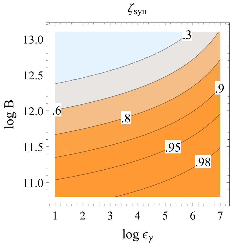
Figure 5.— Fraction of the parent photon energy radiated as synchrotron photons by freshly created pairs: contours of $\zeta_{\textrm{\scriptsize{syn}}}$ as a function of logarithms of the parent photon energy $\epsilon_{\gamma}$ and magnetic field strength $B$ in Gauss for $\rho_{\textrm{\scriptsize{c}}}=10^{7}\mbox{cm}$.

It is evident from Fig. 5 that for higher magnetic field strengths, $B\gtrsim\mbox{$3\times 10^{12}$}\mbox{G}$, and lower energies of parent photons, a progressively smaller fraction of the parent photon energy goes into synchrotron photons; the rest remains in the kinetic energy of the created pairs moving along magnetic field lines. The portion of the parent photon energy energy left in kinetic energy of pairs does not go into production of next generation pairs but is “lost” from the synchrotron cascade. The reason for this is that for higher magnetic field strengths pairs are created when the photon has a smaller pitch angle $\psi_{a}$, so that a smaller fraction of the photon energy goes into perpendicular pair energy, and hence, a smaller fraction of the photon energy is emitted and remains in the cascade.

4.2. Number of secondary photons

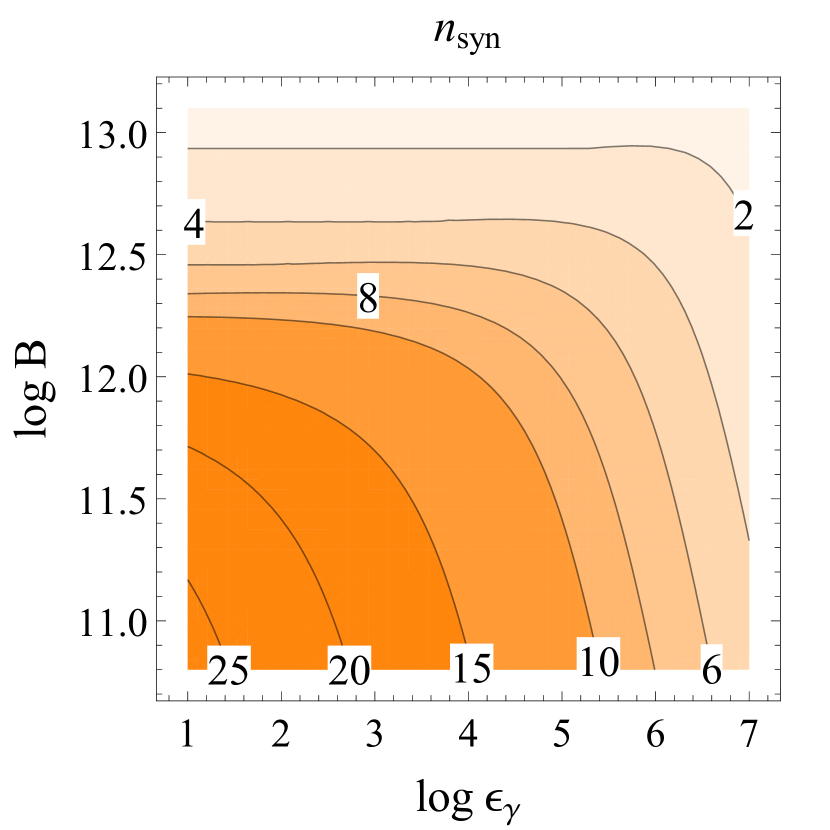
Figure 6.— Number of synchrotron photons with the characteristic energy $\epsilon_{\gamma,\,\textrm{\scriptsize{syn}}}$ emitted at each $\gamma\rightarrow{}e^{+}e^{-}$ conversion: contours of $n_{\textrm{\scriptsize{syn}}}$ as a function of logarithms of the parent photon energy $\epsilon_{\gamma}$ and magnetic field strength $B$ in Gauss for $\rho_{\textrm{\scriptsize{c}}}=10^{7}\mbox{cm}$.

At each pair creation event the parent photon is effectively transformed into an electron-positron pair and lower energy synchrotron photons. Those photons become parent photons for the next cascade generation or escape the magnetosphere, terminating the cascade.

The characteristic energy of synchrotron photons emitted by a newly created particle in terms of quantities used in this paper is given by

$$\epsilon_{\gamma,\,\textrm{\scriptsize{syn}}}=\frac{3}{2}b\,\psi_{a}\epsilon_{\pm,\,\textrm{\scriptsize{{i}}}}^{2}.$$ (14)

The number of synchrotron photons with the characteristic energy $\epsilon_{\gamma,\,\textrm{\scriptsize{syn}}}$ – these photons carry most of the energy of synchrotron radiation – emitted at each event of conversion of a parent photon with energy $\epsilon_{\gamma}$ into an electron-positron pair is

$$n_{\textrm{\scriptsize{syn}}}\simeq\frac{\zeta_{\textrm{\scriptsize{syn}}}\,\epsilon_{\gamma}}{\epsilon_{\gamma,\,\textrm{\scriptsize{syn}}}}=\frac{4}{3}\frac{\zeta_{\textrm{\scriptsize{syn}}}}{\chi_{a}}.$$ (15)

In eq. (15) both $\zeta_{\textrm{\scriptsize{syn}}}$ and $\chi_{a}$ are functions of $B$, $\epsilon_{\gamma}$, and $\rho_{\textrm{\scriptsize{c}}}$. In Fig. 6 we plot contours of $n_{\textrm{\scriptsize{syn}}}$ as functions of the photon energy and magnetic field strength, the radius of curvature was assumed to be $\rho_{\textrm{\scriptsize{c}}}=10^{7}\mbox{cm}$. Two clear trends are visible on this plot: the lower the energy of the primary photon the larger the number of secondary synchrotron photons produced at each conversion event, and the higher the magnetic field the smaller is the number of synchrotron photons. The first one is a general trend of emission processes when higher energy particles emit less photons which, however, have larger energies. The second trend is due to the suppression of the synchrotron cascade discussed above, in §4.1.

4.3. Multiplicity of synchrotron cascade

The generation $i+1$ cascade photon is a synchrotron photon emitted at the event of pair creation by a photon of generation $i$. Expressing $b$, $\psi_{a}$ and $\epsilon_{\gamma}^{(i)}$ through $\chi_{a}$ and $\epsilon_{\gamma}$ from eq. (14) we get for the characteristic energy of the next generation photon

$$\epsilon_{\gamma}^{(i+1)}=\frac{3}{4}\chi_{a}\epsilon_{\gamma}^{(i)}\,,$$ (16)

where $\epsilon_{\gamma}^{(i)}$ and $\epsilon_{\gamma}^{(i+1)}$ are energies of $i$’th and $(i+1)$’th generation photons. The photon energy degrades with each successive generation of the cascade. This degradation accelerates as the cascade proceeds through generations because with the decrease of the photon energy $\chi_{a}$ increases, see Fig. 2.

The photon mfp in a constant magnetic field goes as $l_{\gamma}\propto\chi_{a}/\epsilon_{\gamma}$. For photon energies $\epsilon_{\gamma}\lesssim{}10^{4}$, when $\chi_{a}\gtrsim{}10$, the mfp of successive generations increases by at least an order of magnitude in each successive generation; therefore the crudeness of our approximation for estimating the energy of escaping photons, eq. (10), could affect only the last cascade generation.

The rapid energy degradation results in a rather small number of generations in polar cap cascades as the energy of pair-producing photons rapidly reaches the threshold energy. On the other hand, the number of emitted synchrotron photons increases with the decrease of the energy of the parent photon, see Fig. 6; consequently synchrotron cascades can have quite large multiplicities despite a small number of generations.

Each cascade photon creates 2 particles at the moment of absorption, and particles are produced until $\epsilon_{\gamma}^{(i+1)}\geq\epsilon_{\gamma,\,\textrm{\scriptsize{esc}}}$. The total number of particles generated in synchrotron cascades initiated by a primary photon can be calculated by summation over all generations of the number of pairs produced in each cascade generation. The algorithm for this calculation is shown in Appendix A, algorithm 1. We will use this algorithm for calculation of the polar cap cascade multiplicity after we discuss curvature radiation, the radiation mechanism responsible for generating the primary photons for synchrotron cascades in young energetic pulsars.

Finally we wish to point out how the magnetic field strength affects the multiplicity of the synchrotron cascade. From discussions presented in §§3.2, 4.1 it is evident that, for the same energy of the primary photon, a higher magnetic field strength results in (i) reducing the final energy of escaping photons, therefore increasing cascade efficiency, and at the same time (ii) in suppression of cascade efficiency by forcing a smaller fraction of the photon energy to go into perpendicular energy of the created pairs and so short-circuiting the cascade. Therefore, there should be a “sweet spot” in magnetic field strength where the synchrotron cascade is most efficient.

5. Curvature Radiation

In this section we discuss how primary particles emit photons which “launch” the synchrotron cascade. As we discussed above the most efficient process for supplying the primary (generation 0) photons in young energetic pulsars is curvature radiation.

5.1. Fraction of the primary particle energy going into the cascade

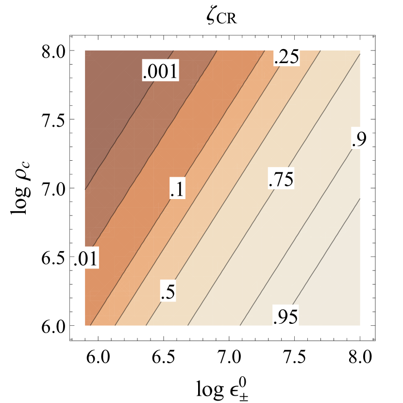
Figure 7.— Fraction of the primary particle energy emitted as CR photons over the distance $s_{\textrm{\scriptsize{{cr}}}}=1$: contours of $\zeta_{\textrm{\scriptsize{{cr}}}}$ as a function of logarithms of the initial particle energy $\epsilon_{\pm}^{0}$ and the radius of curvature of magnetic field lines $\rho_{\textrm{\scriptsize{c}}}$ in cm.

Ultrarelativistic particles moving along curved magnetic field lines emit electromagnetic radiation with power (Jackson, 1975)

$$P_{\textrm{\scriptsize{{cr}}}}=\frac{2}{3}\frac{e^{2}}{m_{e}c^{5}}\left(\frac{c^{2}}{\rho_{\textrm{\scriptsize{c}}}}\right)^{2}\epsilon_{\pm}^{4}\,,$$ (17)

where $P_{\textrm{\scriptsize{{cr}}}}$ is normalized to $m_{e}c^{2}/\mbox{sec}$, $\epsilon_{\pm}$ is the particle’s energy normalized to $m_{e}c^{2}$; we do not distinguish between electrons and positrons. Since we are treating the pair generation problem separately from the problem of particle acceleration, we consider cascades produced by particles injected in a region with screened electric field, so that particles are not accelerated and only lose energy to CR. The particle’s energy decreases with time according to the equation of motion

$$\frac{d\epsilon_{\pm}}{dt}=-P_{\textrm{\scriptsize{{cr}}}}.$$ (18)

Solving eq. (18) we get for the particle energy after it travels the distance $s$ from the injection point

$$\epsilon_{\pm}(s)=\epsilon_{\pm}^{0}\left[1+3H\frac{(\epsilon_{\pm}^{0})^{3}}{\rho_{\textrm{\scriptsize{c}}}^{2}}s\right]^{-1/3}$$ (19)

(see also Harding, 1981), where $s$ is normalized to $R_{\textrm{\scriptsize{{ns}}}}$, $\epsilon_{\pm}^{0}$ is the initial particle energy; constant $H$ is defined as $H=(2/3)R_{\textrm{\scriptsize{{ns}}}}{}r_{e}\approx\mbox{$1.88\times 10^{-7}$}\mbox{cm}^{2}$, where $r_{e}=e^{2}/m_{e}c^{2}$ is the classical electron radius.

The fraction $\zeta_{\textrm{\scriptsize{{cr}}}}$ of the initial particle energy lost to curvature radiation after a particle has traveled distance $s_{\textrm{\scriptsize{{cr}}}}$ is

$$\zeta_{\textrm{\scriptsize{{cr}}}}(s_{\textrm{\scriptsize{{cr}}}})=1-\frac{\epsilon_{\pm}(s_{\textrm{\scriptsize{{cr}}}})}{\epsilon_{\pm}^{0}}.$$ (20)

If the energy of these CR photons goes into creation of electron-positron pairs, $\zeta_{\textrm{\scriptsize{{cr}}}}$ gives the efficiency of the CR part of the full cascade. The electric field in the acceleration zone transforms electromagnetic energy into particle’s kinetic energy, which is then radiated as pair producing photons. Only the photon’s energy can be divided in chunks carried by a large number of pairs. The cascade will have high efficiency if (i) primary particles have high energy, (ii) emit most of their energy as photons, and (iii) inject these photons in the region where the synchrotron cascade can work effectively, i.e. in a region close to the NS which is smaller than the characteristic scale of magnetic field variation $L_{B}$.

In Fig. 7 we plot the fraction of the primary particle energy emitted as CR photons after the particle has traveled distance $s_{\textrm{\scriptsize{{cr}}}}=1$. Shown are contours of $\zeta_{\textrm{\scriptsize{{cr}}}}(s_{\textrm{\scriptsize{{cr}}}})$ as a function of the initial particle energy $\epsilon_{\pm}^{0}$ and the radius of curvature of magnetic field lines $\rho_{\textrm{\scriptsize{c}}}$. For smaller values of $s_{\textrm{\scriptsize{{cr}}}}$ the whole plot would move to the right. CR is most efficient in transferring particle energy into the cascade in the parameter space corresponding to the lower right triangular region of Fig. 7. Going from the upper left (smaller $\epsilon_{\pm}^{0}$, larger $\rho_{\textrm{\scriptsize{c}}}$) to the lower right (larger $\epsilon_{\pm}^{0}$, smaller $\rho_{\textrm{\scriptsize{c}}}$) on this plot, not only the particle energy increases but also the fraction of the energy which can go into the cascade.

For a certain range of $\epsilon_{\pm}^{0}$ and $\rho_{\textrm{\scriptsize{c}}}$ the energy put into the cascade by the primary particle grows faster than the energy of that particle, i.e. the fraction of particle’s energy going into the cascade increases stronger than linearly with the energy of the particle. For more or less regular global magnetic fields, with $\rho_{\textrm{\scriptsize{c}}}\gtrsim 10^{7}\mbox{cm}$, the transition between effective and ineffective CR cascades occurs at particle energies $\epsilon_{\pm}\sim 10^{7}$, and the efficiency is very sensitive to the particle energy. In this parameter range even a modest increase of the primary particle energy can result in a large boost of the cascade multiplicity.

5.2. Energy of CR photons and critical particle energy

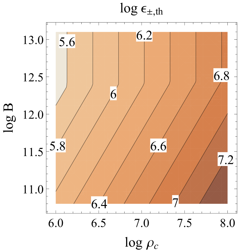
Figure 8.— Critical particle energy above which it can emit pair-producing photons via curvature radiation: contours of $\log\epsilon_{\pm,\,\textrm{\scriptsize{th}}}$ as a function of logarithms of the radius of curvature of magnetic field lines $\rho_{\textrm{\scriptsize{c}}}$ in cm and magnetic field strength $B$ in Gauss for $s_{\textrm{\scriptsize{esc}}}=1$.

The characteristic energy of CR photons emitted by a particle with the energy $\epsilon_{\pm}$ is (Jackson, 1975)

$$\epsilon_{\gamma,\,\textrm{\scriptsize{{cr}}}}=\frac{3}{2}\frac{\lambdabar{}_{\textrm{\scriptsize{{c}}}}}{\rho_{\textrm{\scriptsize{c}}}}\epsilon_{\pm}{}^{3}\approx\mbox{$5.8\times 10^{3}$}\,\rho_{\textrm{\scriptsize{c,\,7}}}^{-1}\>\epsilon_{\pm,\,\textrm{\scriptsize{7}}}^{3}\,,$$ (21)

where $\rho_{\textrm{\scriptsize{c,\,7}}}\equiv{}\rho_{\textrm{\scriptsize{c}}}/10^{7}\mbox{cm}$ and $\epsilon_{\pm,\,\textrm{\scriptsize{7}}}\equiv\epsilon_{\pm}/10^{7}$. The number of CR photons emitted by the particle while traveling distance $ds$ normalized to $R_{\textrm{\scriptsize{{ns}}}}$ is

$$\frac{d\,n_{\textrm{\scriptsize{{cr}}}}}{ds}\simeq\frac{R_{\textrm{\scriptsize{{ns}}}}}{c}\frac{P_{\textrm{\scriptsize{{cr}}}}}{\epsilon_{\gamma,\,\textrm{\scriptsize{{cr}}}}}$$ (22)

Each CR photon above the pair formation threshold will be a primary photon for the synchrotron cascade discussed in §4. The critical energy at which primary particles can produce pair-creating CR photons can be calculated by equating $\epsilon_{\gamma,\,\textrm{\scriptsize{{cr}}}}$ given by eq. (21) to the escape photon energy $\epsilon_{\gamma,\,\textrm{\scriptsize{esc}}}$ from eq. (10). In Fig. 8 we plot the critical particle energy which could initiate pair production with CR photons $\epsilon_{\pm,\,\textrm{\scriptsize{th}}}$ for $s_{\textrm{\scriptsize{esc}}}=1$. Shown are contours of $\log\epsilon_{\pm,\,\textrm{\scriptsize{th}}}$ as a function of the radius of curvature of magnetic field lines $\rho_{\textrm{\scriptsize{c}}}$ and magnetic field strength $B$. Primary particles should have energies $\epsilon_{\pm}\gtrsim{}10^{6}$ to be able to initiate pair production via CR.

5.3. Multiplicity of CR-synchrotron cascade

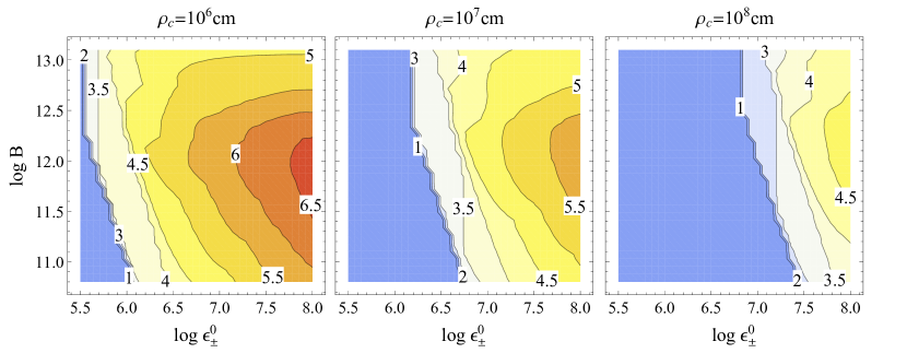
Figure 9.— Multiplicity of CR-synchrotron cascade: contours of $\log\kappa_{\textrm{\scriptsize{{cr}-syn}}}$ as a function of logarithms of the primary particle energy $\epsilon_{\pm}^{0}$ and magnetic field strength $B$ in Gauss for three values of the radius of curvature of magnetic field lines $\rho_{\textrm{\scriptsize{c}}}=10^{6},10^{7},10^{8}\mbox{cm}$. Assumed values for characteristic lengths: $s_{\textrm{\scriptsize{{cr}}}}=s_{\textrm{\scriptsize{esc}}}=1$.

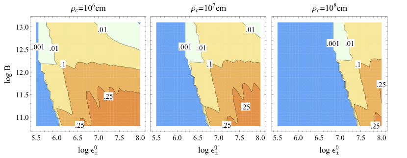
Figure 10.— Efficiency of CR-synchrotron cascade as given by eq. (24): contours of $\zeta_{\textrm{\scriptsize{{cr}-syn}}}$ as a function of logarithms of the primary particle energy $\epsilon_{\pm}^{0}$ and magnetic field strength $B$ in Gauss for three values of the radius of curvature of magnetic field lines $\rho_{\textrm{\scriptsize{c}}}=10^{6},10^{7},10^{8}\mbox{cm}$. Assumed values for characteristic lengths: $s_{\textrm{\scriptsize{{cr}}}}=s_{\textrm{\scriptsize{esc}}}=1$.

The multiplicity of the the CR-synchrotron cascade – the total number of particles produced by a single primary electron or positron accelerated in the gap – can be computed by multiplying the number of CR photons $n_{\textrm{\scriptsize{{cr}}}}$, eq. (22), by the number of particles produced in the synchrotron cascade initiated by these photons $n_{\textrm{\scriptsize{syn}}}$, eq. (15), and integrating it over the distance where CR can initiate a cascade

$$\kappa_{\textrm{\scriptsize{{cr}-syn}}}=\int_{0}^{s_{\textrm{\scriptsize{{cr}}}}}n_{\textrm{\scriptsize{syn}}}\frac{d\,n_{\textrm{\scriptsize{{cr}}}}}{ds}\,ds\,.$$ (23)

The actual algorithm we use to compute the total multiplicity is the Algorithm 2 from Appendix A. Integration in eq. (23) is done assuming constant values for $B$ and $\rho_{\textrm{\scriptsize{c}}}$, as discussed in § 3.1. In Fig. 9 we plot $\kappa_{\textrm{\scriptsize{{cr}-syn}}}$ as a function of the initial particle energy $\log\epsilon_{\pm}^{0}$ and magnetic field strength $\log{}B$ for three different radii of curvature of magnetic field lines $\rho_{\textrm{\scriptsize{c}}}=10^{6},10^{7},10^{8}$ cm assuming $s_{\textrm{\scriptsize{{cr}}}}=s_{\textrm{\scriptsize{esc}}}=1$.

It is evident from these plots that in a dipolar magnetic field, with $\rho_{\textrm{\scriptsize{c}}}\approx 10^{8}\mbox{cm}$, the maximum achievable multiplicity is $\kappa_{\textrm{\scriptsize{{cr}-syn}}}\sim\mbox{$\mbox{few}\times 10^{4}$}$ even in cascades initiated by extremely energetic primary particles. If the radius of curvature is an order of magnitude less, a rather high multiplicity $\kappa_{\textrm{\scriptsize{{cr}-syn}}}\gtrsim 10^{5}$ could be achieved in polar cap cascades for magnetic field strength $B\sim 10^{12}$ G and particle energies $\epsilon_{\pm}\gtrsim 10^{7}$, parameters quite realistic for young pulsars. For strongly non-dipolar magnetic field, with $\rho_{\textrm{\scriptsize{c}}}\approx 10^{6}\mbox{cm}$ the multiplicity can be another order of magnitude higher $\kappa_{\textrm{\scriptsize{{cr}-syn}}}\sim\mbox{$\mbox{few}\times 10^{6}$}$.

The properties of CR do not depend on the strength of the magnetic field, therefore the effect of the magnetic field strength on the multiplicity of CR-synchrotron cascade is due to the synchrotron cascade and how many CR photons pair produce. As discussed at the end of § 4.3 there should be an optimum magnetic field strength where the multiplicity is the highest; the multiplicity decreases both for higher (due to larger energy left in particle motion along magnetic field lines) as well as lower magnetic field (due to increase of the energy of escaping photons). This trend is clearly visible on all plots of Fig. 9. The highest cascade multiplicity is achieved for magnetic field around $B\sim 10^{12}$ G. The value of this optimum magnetic field grows slightly with increase of $\rho_{\textrm{\scriptsize{c}}}$, but it stays around $\sim\mbox{$\mbox{few}\times 10^{12}$}$ G even for dipolar magnetic fields. This is noteworthy in view of the fact that $B\sim 10^{12}$ G is the typical value of magnetic field strength for normal pulsars. For any given energy of the primary particle the decrease of the cascade multiplicity towards stronger magnetic fields is faster than for weaker fields.

The dependence of cascade multiplicity on the initial energy of the primary particle is non-linear. Let us consider what happens when the initial particle energy $\epsilon_{\pm}^{0}$ goes from the highest to the lowest value (horizontal direction in plots of Fig. 9). For the highest values of $\epsilon_{\pm}^{0}$ multiplicity decreases uniformly, but then it drops by an order of magnitude in a rather small range of $\epsilon_{\pm}^{0}$ (for $B\sim 10^{12}$G it happens around $\epsilon_{\pm}^{0}\sim 10^{6.3}$ for $\rho_{\textrm{\scriptsize{c}}}=10^{6}$cm, $\epsilon_{\pm}^{0}\sim 10^{6.8}$ for $\rho_{\textrm{\scriptsize{c}}}=10^{7}$cm, and $\epsilon_{\pm}^{0}\sim 10^{7.4}$ for $\rho_{\textrm{\scriptsize{c}}}=10^{8}$cm). After about half a decade of $\epsilon_{\pm}^{0}$ values the multiplicity drops again to 1, when no particles can be produced (for $B\sim 10^{12}$G it happens around $\epsilon_{\pm}^{0}\sim 10^{5.7}$ for $\rho_{\textrm{\scriptsize{c}}}=10^{6}$cm, $\epsilon_{\pm}^{0}\sim 10^{6.3}$ for $\rho_{\textrm{\scriptsize{c}}}=10^{7}$cm, and $\epsilon_{\pm}^{0}\sim 10^{7}$ for $\rho_{\textrm{\scriptsize{c}}}=10^{8}$cm). The first effect is due to the decrease of the efficiency of CR, discussed in §5.1. For lower initial energies of the primary particle there is less energy available to create pairs, not only because the particle energy is smaller, but also due to smaller efficiency of CR in producing photons – the primary particle keeps most of its energy, depositing only a small fraction of it in the cascade zone. The drop in the efficiency of CR $\zeta_{\textrm{\scriptsize{{cr}}}}$, where it becomes less than 10% (see Fig. 7) manifests in a rapid decrease of cascade multiplicity – by an order of magnitude – on all plots of Fig. 9 for magnetic field strengths where the maximum multiplicity is achieved. This drop in $\kappa_{\textrm{\scriptsize{{cr}-syn}}}$ is most prominent for $B\sim 10^{12}$G and is less pronounced for both higher and lower magnetic field strengths due to lower efficiency of the cascade discussed above. The second drop in $\kappa_{\textrm{\scriptsize{{cr}-syn}}}$, towards 1, is due to the threshold in pair formation – for those particle energies CR photons have too low an energy to initiate a cascade. The blue region on the plots of Fig. 9 show the parameter space where no particles can be produced by the CR-synchrotron cascade. It does not mean, however, that no pairs can be produced in the polar cap cascades for such primary particle energies. Instead of CR, the primary photons for synchrotron cascade will be produced by inverse Compton scattering of thermal photons emitted by the NS, however, those primary photons will have much lower energies and multiplicities of such cascades will be quite low (see Harding & Muslimov, 2002).

We find it also instructive to compare the multiplicity of the CR-synchrotron cascade with the theoretical upper limit on cascade multiplicity $\kappa_{\textrm{\scriptsize{max}}}$, given by eq. (1) in §2. The ratio

$$\zeta_{\textrm{\scriptsize{{cr}-syn}}}=\frac{\kappa_{\textrm{\scriptsize{{cr}-syn}}}}{\kappa_{\textrm{\scriptsize{max}}}}$$ (24)

can be considered as the efficiency of splitting the energy of the primary particle into pairs. In Fig. 10 we plot $\zeta_{\textrm{\scriptsize{{cr}-syn}}}$ for the same values of parameters as $\kappa_{\textrm{\scriptsize{{cr}-syn}}}$ in Fig. 9. Despite lower multiplicity for smaller values of $B$, the cascade efficiency is higher, i.e. more of the initial energy of the primary particle goes into pair formation as opposed to the energy of escaping photons and kinetic energy of pairs and primary particles. This trend is discussed in §4.1, 5.1. It is interesting to note that for $B\lesssim\mbox{$\mbox{few}\times 10^{11}$}$ G the cascade can be quite efficient in splitting a noticeable fraction of primary particle energy into pairs. For magnetic field $\sim 10^{12}$ G the fraction of the primary particle’s energy going into pair production saturates at $\sim 10\%$; this is the limiting efficiency of the highest possible multiplicity cascade in a typical pulsar. The dependence of $\zeta_{\textrm{\scriptsize{{cr}-syn}}}$ on $\epsilon_{\pm}^{0}$ is similar to the dependence of $\kappa_{\textrm{\scriptsize{{cr}-syn}}}$ on $\epsilon_{\pm}^{0}$.

6. Particle acceleration

6.1. Overview of particle acceleration regimes

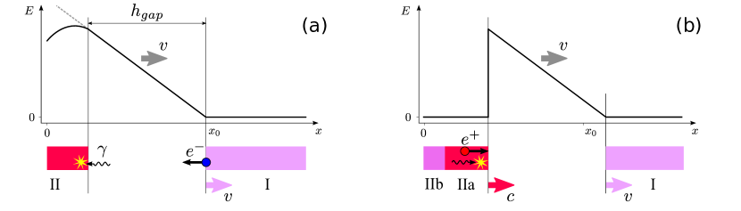
Figure 11.— Schematic representation of gap formation and evolution for cascades in Ruderman-Sutherland regime with $j_{\textrm{\scriptsize{m}}}/j_{\textrm{\scriptsize{{gj}}}}>0$. See text for explanation.

In this section we will get an estimate for the energy of primary cascade particles. In the following discussion we will rely on results of self-consistent modeling of pair cascades by Timokhin (2010) [T10] and Timokhin & Arons (2013) [TA13]. First, we give a brief overview of how particle acceleration proceeds according to these simulations.

Whether and how the pair formation along given magnetic field lines occurs depends on the ratio $j_{\textrm{\scriptsize{m}}}/j_{\textrm{\scriptsize{{gj}}}}$ of the current density required to support the twist of magnetic field lines in the pulsar magnetosphere (e.g. Timokhin, 2006; Bai & Spitkovsky, 2010), $j_{\textrm{\scriptsize{m}}}\equiv(c/4\pi)\,|\nabla\times\mathbf{B}|$, to the local GJ current density, $j_{\textrm{\scriptsize{{gj}}}}\equiv\eta_{\textrm{\scriptsize{{gj}}}}c$, where $\eta_{\textrm{\scriptsize{{gj}}}}=B/Pc$ is the GJ charge density.

For the Ruderman & Sutherland (1975) cascade model, where particles cannot be extracted from the NS surface, effective particle acceleration and pair formation is possible for almost all values of $j_{\textrm{\scriptsize{m}}}/j_{\textrm{\scriptsize{{gj}}}}$ (T10). In the space charge limited flow regime, first discussed by Arons & Scharlemann (1979), pair formation is not possible if $0<j_{\textrm{\scriptsize{m}}}/j_{\textrm{\scriptsize{{gj}}}}<1$, but is possible for all other values of $j_{\textrm{\scriptsize{m}}}/j_{\textrm{\scriptsize{{gj}}}}$ (TA13). Pair formation is always non-stationary: an active phase when particles are accelerated to ultrarelativistic energies and give rise to electron-positron cascades – with a burst of pair formation – is followed by a quiet phase when recently generated dense electron-positron plasma screens the electric field everywhere.

As pair plasma leaves the active region, it flows into the magnetosphere, and later into the pulsar wind. When the density of the pair plasma drops below the minimum density necessary for screening of the electric field a gap appears – a charge starved region where the electric field is very strong, of the order of the vacuum electric field. To screen the electric field, the plasma density must be high enough to provide both the GJ charge density $\eta_{\textrm{\scriptsize{{gj}}}}$ and the imposed current density $j_{\textrm{\scriptsize{m}}}$. The transition between the region(s) still filled with plasma (hereafter we call it “plasma tail”) and the gap is sharp – plasma still capable of screening the electric field moves in bulk, its density is close to the critical density. The plasma density drops abruptly at the gap boundary; within the gap the particle number density is much smaller than the critical density (cf. Fig. 22, 23 in § 10). The motion of the boundary between the plasma filled region and the gap sets the gap’s growth rate. Some particles enter the gap and are accelerated to ultrarelativistic energies. The gap grows until the energy of particles accelerated there becomes sufficient to start electron-positron cascades and the cycle repeats. The gap is not stationary; in almost all cases it moves as a whole – after its growth has been terminated by newly created pairs its upper and low boundaries are moving in the same direction. The gap can move, keeping its size for a long time, or it might disappear rather quickly. The details of gap behavior – where the gap appears, what direction it moves, how fast it disappears – depend on the ratio $j_{\textrm{\scriptsize{m}}}/j_{\textrm{\scriptsize{{gj}}}}$. However, despite these differences, the way in which the highest energy particles are accelerated is very similar in any regime which allows pair formation studied in T10, TA13. Namely, the size of the charge starved region grows as the tail of pair plasma moves, the bulk velocity of the tail $v$ sets the rate of the gap expansion. Particles entering the gap from the tail are accelerated in a larger and larger gap, until they are able to produce pair-producing photons. The place where these photons are absorbed and produce pairs is the other boundary of the gap.

6.2. Energy of primary particles

In this section we obtain a quantitative estimate for the maximum energy of accelerated particles using as an example the case of the Ruderman-Sutherland (RS) cascade, when particles cannot be supplied from the surface of the NS. As we mentioned before, gap formation and particle acceleration in the space charge limited flow regime, when pair creation is allowed, is very similar to the RS case and estimates for particle energies obtained in this section are applicable for the space charge limited flow with $j_{\textrm{\scriptsize{m}}}/j_{\textrm{\scriptsize{{gj}}}}>1$ and $j_{\textrm{\scriptsize{m}}}/j_{\textrm{\scriptsize{{gj}}}}<0$. The GJ charge density is positive and we consider the case when the ratio $j_{\textrm{\scriptsize{m}}}/j_{\textrm{\scriptsize{{gj}}}}>0$. In Fig. 11 we show a schematic picture of how particles are accelerated in this cascade. On the top of each figure we show the electric field in the accelerating region and on the bottom a schematic representation of plasma motion in and around the gap; plot (a) corresponds to the time when the electric field screening has just started, plot (b) shows a well-developed gap moving into the magnetosphere. These schematic plots illustrate results of actual simulations of RS cascades shown in Fig. 3,4,11 and 13 in T10.

At the beginning of the burst of pair formation, the gap appears at the NS surface and its upper boundary is the “tail” of plasma left from the previous burst of pair formation, where the particle number density is still high enough to screen the electric field (region I in Fig. 11). Electrons and positrons in this tail are trapped in electrostatic oscillations and the bulk velocity of this tail $v$ is sub-relativistic, but for large current densities (around or greater than $j_{\textrm{\scriptsize{{gj}}}}$) it is quite close to $c$. Electrons from this tail which get to the gap boundary are pulled into the gap and are accelerated toward the NS. As the tail moves, the gap grows; the current and charge density in the gap is due to the flux of electrons from the tail and so it remains constant within the gap. The gap growth is stopped when electrons reach an energy high enough to produce pair-creating photons. This first-generation of pairs start screening the electric field – electrons move toward the NS and positrons are accelerated toward the magnetosphere and start producing pair creating photons as well (region II in Fig. 11(a)). In numerical simulations (T10) the first-generation positrons moving toward the magnetosphere have approximately the same energies as the primary electrons which initiated the discharge. Because those positrons are ultrarelativistic they practically co-move with the photons and so new pairs are injected close to their parent particles making a blob of pair plasma moving into the magnetosphere (region IIa in Fig. 11(b)). This blob is the lower boundary of the accelerating gap, and the gap exists until this blob catches up with the tail from the previous pair formation cycle. For large current densities this can take a while as $v$ is close to $c$. Plasma leaking from the blob forms the new tail (region IIb on Fig. 11(b)).

In the discharge described above primary particles are moving in both directions and initiate cascades toward the NS (electrons) and the magnetosphere (positrons). As the discharges happen close to the NS surface, the cascade can fully develop only in the direction of the magnetosphere – particles moving toward NS slam onto the star’s surface before they can produce a lot of pairs. For RS discharges the primary, generation 0, particles initiating the full cascade in Fig. 1 are positrons in region IIa in Fig. 11(b). As we mentioned above, the energy of those positrons is very close to the energy of the primary electrons and here, for the sake of simplicity, we provide estimates only for the energy of primary electrons.

The evolution of the electric field in any given point $x$ and moment of time $t$ is given by (see e.g. eq. 1 in TA13)

$$\frac{\partial{E}}{\partial{t}}(x,t)=-4\pi\left(j(x,t)-j_{\textrm{\scriptsize{m}}}\right)\equiv-4\pi\tilde{\jmath}\,,$$ (25)

$j$ is the actual current density along a given magnetic field line and $j_{\textrm{\scriptsize{m}}}$ is the current density imposed by the magnetosphere. The difference $\tilde{\jmath}\equiv{}j-j_{\textrm{\scriptsize{m}}}$ in the gap remains constant. When the upper boundary of the gap moves with the constant speed $v$ this equation can be integrated to get the electric field in the gap

$$E(x,t)=E(x_{0},t_{0})+4\pi\tilde{\jmath}\,\frac{x_{0}-x}{v}+4\pi\tilde{\jmath}\,(t-t_{0})$$ (26)

Where $E(x_{0},t_{0})$ is the electric field within the gap at the moment $t_{0}$ at the point $x_{0}$. If we assume that the gap boundary is at $x_{0}$ at the moment $t_{0}$, then $E(x_{0},t_{0})=0$.

Electrons enter the gap from above and are quickly accelerated by the strong electric field and move with relativistic speed practically from the moment they leave the plasma tail. If a particle enters the gap at $t_{0}$ (in point $x_{0}$) its coordinate is $x_{\pm}=x_{0}-c(t-t_{0})$, substituting $x_{\pm}$ into eq. (26) the electric field seen by that particle is given by

$$E(x_{p})=\frac{4\pi}{c}\tilde{\jmath}\,\left(1+\frac{c}{v}\right)\left(x_{0}-x_{\pm}\right)\equiv 4\pi\eta_{\textrm{\scriptsize{{gj}}}}^{0}\,\xi_{j}\,l_{\pm}$$ (27)

In the last step in eq. (27) we denote with $l_{\pm}\equiv|x_{\pm}-x_{0}|$ the distance traveled by the particle in the gap and introduce $\xi_{j}$ defined as

$$\xi_{j}\equiv\frac{\tilde{\jmath}}{j_{\textrm{\scriptsize{{gj}}}}^{0}}\left(1+\frac{c}{v}\right)\,,$$ (28)

where $j_{\textrm{\scriptsize{{gj}}}}^{0}$ is the GJ current density in an aligned rotator

$$j_{\textrm{\scriptsize{{gj}}}}^{0}\equiv\eta_{\textrm{\scriptsize{{gj}}}}^{0}c=\frac{B}{P}\,.$$ (29)

$\xi_{j}$ is a factor which shows how stronger/weaker the electric field in the gap is compared to the situation of a static vacuum gap in an (anti-)aligned rotator, like the one considered by Ruderman & Sutherland (1975). $v\simeq\mbox{const}$ is a good approximation to the numerical results and so $\xi_{j}\simeq\mbox{const}$. In cascades along magnetic field lines where $j_{\textrm{\scriptsize{m}}}$ is close to the local value of $j_{\textrm{\scriptsize{{gj}}}}$ in an aligned rotator $\xi_{j}\sim 2$, for the same situation in a pulsar with inclination angle of $60^{\circ}$, $\xi_{j}\sim 1$.

For energy losses dominated by curvature radiation, free acceleration is a good approximation for $B\gtrsim{}10^{11}$ G (see Appendix B). If radiation losses are negligible, the particle’s equation of motion is

$$\frac{dp}{dt}=-eE\,,$$ (30)

where $p=mc\gamma$ is particle’s momentum. In terms of the distance traveled by the particle in the gap $l_{\pm}=c(t-t_{0})$ with $E$ given by eq. (27), particle equation of motion can be written as

$$\frac{dp}{dl_{\pm}}=\frac{4\pi e}{c}\eta_{\textrm{\scriptsize{{gj}}}}^{0}\xi_{j}\,l_{\pm}\,.$$ (31)

Integrating this equation and expressing $j_{\textrm{\scriptsize{{gj}}}}$ through pulsar parameters we get for particle energy

$$\epsilon_{\pm}=\frac{2\pi}{B_{q}\lambdabar{}_{\textrm{\scriptsize{{c}}}}c}\xi_{j}\frac{B}{P}\,l_{\pm}^{2}$$ (32)

The distance the primary particle travels in the region of unscreened electric field $l_{\textrm{\scriptsize{gap}}}$ – the size of the gap as seen by the moving particle – is the sum of the distance the particle travels before emitting pair-producing photons terminating the gap $l_{\pm,\,\textrm{\scriptsize{gap}}}^{\textrm{\scriptsize{e}}}$ and the distance these protons travel until the absorption point $l_{\gamma,\,\textrm{\scriptsize{gap}}}$

$$l_{\textrm{\scriptsize{gap}}}=l_{\pm,\,\textrm{\scriptsize{gap}}}^{\textrm{\scriptsize{e}}}+l_{\gamma,\,\textrm{\scriptsize{gap}}}\,.$$ (33)

For any given particle, the larger the distance $l_{\pm}^{\textrm{\scriptsize{e}}}$ the particle travels to the emission point, the higher the particle energy and the energy of CR photons it emits, and so the smaller is the distance traveled by the photon until the absorption point $l_{\gamma}$. The distance the particle travels in the gap $l_{\textrm{\scriptsize{gap}}}$ is the minimum value of $l=l_{\pm}^{\textrm{\scriptsize{e}}}+l_{\gamma}$ because once the first pairs are injected the avalanche of pair creation will lead to screening of the electric field. The photon mean free path $l_{\gamma}$ can be estimated from eq. (3) as

$$l_{\gamma}=2\chi_{a}\frac{\rho_{\textrm{\scriptsize{c}}}}{b\epsilon_{\gamma}}\,.$$ (34)

Photon energy $\epsilon_{\gamma}$ depends on the particle energy $\epsilon_{\pm}$ which depends on $l_{\pm}^{\textrm{\scriptsize{e}}}$ according to eq. (32), and so $l_{\gamma}$ is a function of $l_{\pm}^{\textrm{\scriptsize{e}}}$. $l_{\textrm{\scriptsize{gap}}}$ can be found by minimizing $l=l_{\pm}^{\textrm{\scriptsize{e}}}+l_{\gamma}$ using $l_{\pm}^{\textrm{\scriptsize{e}}}$ as an independent variable: $l_{\textrm{\scriptsize{gap}}}$ is the value of $l$ which satisfies $dl/dl_{\pm}^{\textrm{\scriptsize{e}}}=0$, $l_{\gamma,\,\textrm{\scriptsize{gap}}}$ and $l_{\pm,\,\textrm{\scriptsize{gap}}}^{\textrm{\scriptsize{e}}}$ are the values of $l_{\gamma}$ and $l_{\pm}^{\textrm{\scriptsize{e}}}$ where $l$ reaches its minimal value. Using eq. (33) we can write an equation for $l_{\gamma,\,\textrm{\scriptsize{gap}}}$

$$\frac{dl_{\gamma,\,\textrm{\scriptsize{gap}}}}{dl_{\pm,\,\textrm{\scriptsize{gap}}}^{\textrm{\scriptsize{e}}}}=-1\,.$$ (35)

If the photon energy depends on $l_{\pm}^{\textrm{\scriptsize{e}}}$ as $\epsilon_{\gamma}\propto{}(l_{\pm}^{\textrm{\scriptsize{e}}})^{\alpha}$, then eq. (35) is reduced to

$$l_{\pm,\,\textrm{\scriptsize{gap}}}^{\textrm{\scriptsize{e}}}=\alpha{}l_{\gamma,\,\textrm{\scriptsize{gap}}}\,,$$ (36)

where $l_{\gamma,\,\textrm{\scriptsize{gap}}}$ is expressed in terms of $l_{\pm,\,\textrm{\scriptsize{gap}}}^{\textrm{\scriptsize{e}}}$ using eq. (34). $l_{\textrm{\scriptsize{gap}}}$ is then given by

$$l_{\textrm{\scriptsize{gap}}}=\frac{\alpha+1}{\alpha}l_{\pm,\,\textrm{\scriptsize{gap}}}^{\textrm{\scriptsize{e}}}\,.$$ (37)

The final energy of the primary particle is given by eq. (32) with $l_{\pm}=l_{\textrm{\scriptsize{gap}}}$. Please note that because the gap moves, the actual size of the gap (see Fig. 11(a)) is

$$h_{\textrm{\scriptsize{gap}}}=\left(1+\frac{v}{c}\right)l_{\textrm{\scriptsize{gap}}}\,.$$ (38)

The energy of the CR photons depends on the particle energy as $\epsilon_{\pm}^{3}$ (eq. 21), the particle energy depends on $l_{\pm}$ as $l_{\pm}^{2}$ (eq. 32), hence, $\epsilon_{\gamma}\propto{}(l_{\pm}^{\textrm{\scriptsize{e}}})^{6}$ and $\alpha=6$. Substituting expression for $\epsilon_{\pm}$ (eq. 32) into the expression for CR photon energy $\epsilon_{\gamma}$ (eq. 21), the latter into eq. (34), and the resulting expression for $l_{\gamma}$ into eq. (36) with $\alpha=6$ after algebraic transformations we get the following expression for $l_{\pm,\,\textrm{\scriptsize{gap}}}^{\textrm{\scriptsize{e}}}$

$$l_{\pm,\,\textrm{\scriptsize{gap}}}^{\textrm{\scriptsize{e}}}=\left(\frac{B_{q}^{4}\lambdabar{}_{\textrm{\scriptsize{{c}}}}^{2}c^{3}}{\pi^{3}}\right)^{1/7}\chi_{a}^{1/7}\xi_{j}^{-3/7}\rho_{\textrm{\scriptsize{c}}}^{2/7}P^{3/7}B^{-4/7}\,.$$ (39)

The size of the gap as seen by the moving particle according to eq. (37) is

$$l_{\textrm{\scriptsize{gap}}}\simeq\mbox{$2\times 10^{4}$}\>\chi_{a}^{1/7}\xi_{j}^{-3/7}\rho_{\textrm{\scriptsize{c,\,7}}}^{2/7}\,P^{3/7}B_{12}^{-4/7}\mbox{cm}\,,$$ (40)

where $B_{12}\equiv{}B/10^{12}\mbox{G}$ and $\rho_{\textrm{\scriptsize{c,\,7}}}\equiv{}\rho_{\textrm{\scriptsize{c}}}/10^{7}\mbox{cm}$. Substituting $l_{\pm}=l_{\textrm{\scriptsize{gap}}}$ into eq. (32) we get for the final energy of particles accelerated in the gap

$$\epsilon_{\pm,\,\textrm{\scriptsize{acc}}} = \frac{49}{18}\left(\frac{\pi B_{q}}{\lambdabar{}_{\textrm{\scriptsize{{c}}}}^{3}c}\right)^{1/7}\chi_{a}^{2/7}\;\xi_{j}^{1/7}\rho_{\textrm{\scriptsize{c}}}^{4/7}P^{-1/7}B^{-1/7}$$ (41)

$$\simeq \mbox{$5\times 10^{7}$}\>\chi_{a}^{2/7}\;\xi_{j}^{1/7}\rho_{\textrm{\scriptsize{c,\,7}}}^{4/7}P^{-1/7}B_{12}^{-1/7}\,.$$

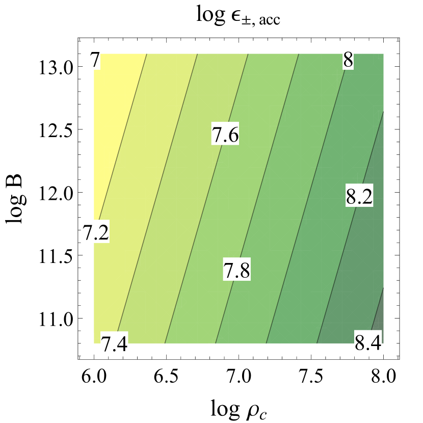
Figure 12.— Primary particle energy: contours of $\log\epsilon_{\pm,\,\textrm{\scriptsize{acc}}}$ as a function of logarithms of the radius of curvature of magnetic field lines $\rho_{\textrm{\scriptsize{c}}}$ in cm and magnetic field strength $B$ in Gauss. We used the following values for gap parameters $P=33$ ms, $\xi_{j}=2$ and $\chi_{a}=1/7$.

The dependence of the primary particles energy on pulsar period $P$, filling factor $\xi_{j}$ and the strength of the magnetic field $B$ is very weak, the only substantial dependence is on the radius of curvature of magnetic field lines. The reason for this is the strong dependence of CR photon energy on the energy of emitting particles $\epsilon_{\gamma}\propto\epsilon_{\pm}^{3}$, eq. (21). Changes in the threshold energy of pair producing photons which can stop the gap growth cause only modest variation of the energy of primary particles, which explicitly depends on $P$, $\xi_{j}$ and $B$, but not on $\rho_{\textrm{\scriptsize{c}}}$, eq. (32). The energy of pair producing photons sets the energy of accelerated particles, and in pulsars with a strong accelerating electric field the gap will be smaller than in pulsars with a weaker accelerating field. In Fig. 12 we plot the energy of particles $\epsilon_{\pm,\,\textrm{\scriptsize{acc}}}$ accelerated in the gap of a pulsar with $P=33$ ms as a function of the radius of curvature of magnetic field lines $\rho_{\textrm{\scriptsize{c}}}$ and magnetic field strength $B$, assuming $\xi_{j}=2$ and $\chi_{a}=1/7$. The value $\chi_{a}\approx 1/7$ corresponds to $\chi_{a}$ of CR photons emitted by relativistic particles with $\epsilon_{\pm}^{0}=\mbox{$2.5\times 10^{7}$}$ in a magnetic field $B=10^{12}$ G with $\rho_{\textrm{\scriptsize{c}}}=10^{7}$ cm, this is a good estimate for $\chi_{a}$ in eq. (41) for young pulsars as the dependence on $\chi_{a}$ is very weak. This plot clearly illustrates the dependence of $\epsilon_{\pm,\,\textrm{\scriptsize{acc}}}$ on $B$ and $\rho_{\textrm{\scriptsize{c}}}$ – weaker magnetic field and/or larger radius of curvature requires larger photon energies for terminating gap growth, and so the energy of the primary particles is larger.

We derived eq. (41) under the following assumptions: (i) particles are accelerated freely, i.e. radiation reaction can be neglected, (ii) the length of the gap is much smaller that the polar cap radius, so that a one dimensional approximation can be used, (iii) the magnetic field is $B\lesssim{}0.2B_{q}\approx\mbox{$8.8\times 10^{12}$}$ G so that the opacity to $\gamma{}B$ pair creation is described by eq. (2). Constraints on the pulsar parameters (i) and (ii) are derived in Appendix B and Appendix C correspondingly. Plotted on the $P\dot{P}$ diagram, Fig. 13, these restrictions select the range of pulsar period and period derivatives – shown as yellow region – where all three assumptions are valid. In this figure, the one-dimensional approximation (ii) is valid to the left of the solid line, given by eq. (C5), the approximation (i) of free acceleration above the dot-dashed line, given by eq. (B2), and pulsars with $B<0.2B_{q}$ are below the dotted line. We see that most of young normal pulsars, including gamma-ray pulsars from the Fermi second pulsar catalog, fall in this range.

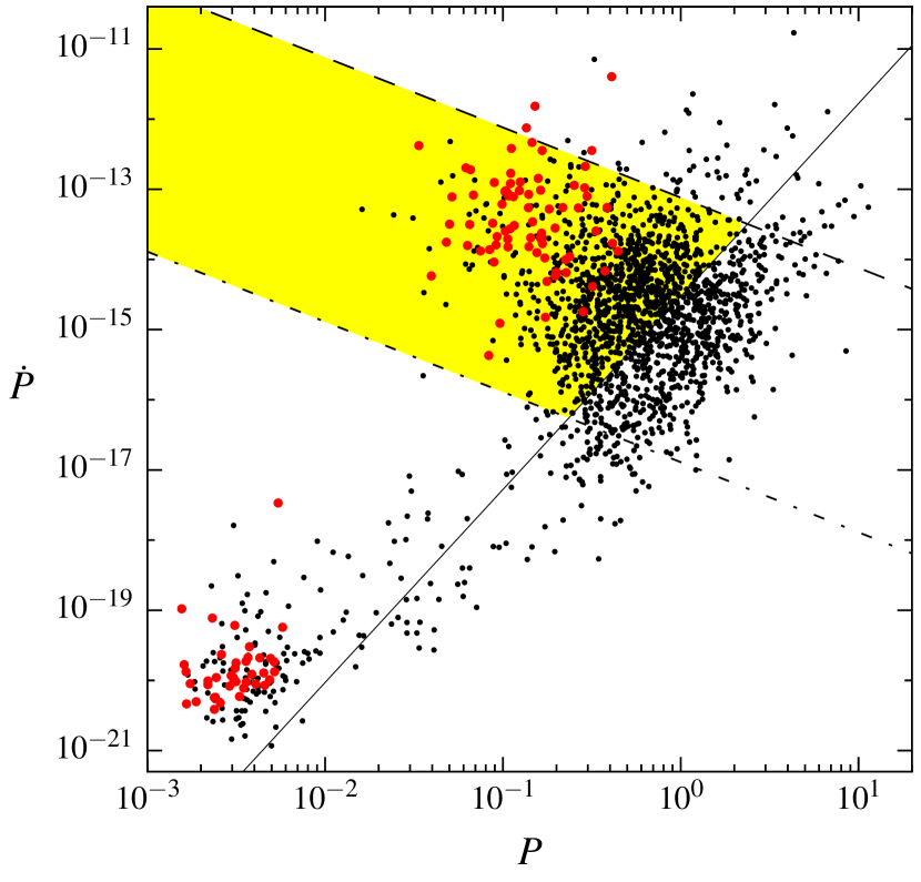
Figure 13.— $P\dot{P}$ diagram with the yellow area showing the range of parameters where approximation for particle acceleration used in this paper is applicable, see text for description. Pulsars from ATNF catalog (Manchester et al. (2005), http://www.atnf.csiro.au/research/pulsar/psrcat) are shown by black dots, $\gamma$-ray pulsars from the second Fermi catalog (Abdo et al., 2013) by red dots.

7. Cascade multiplicity per primary particle: semi-analytical model

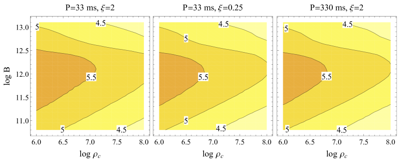
Figure 14.— Multiplicity of polar cap cascades: contours of $\log\kappa$ as a function of logarithms of curvature of magnetic field lines $\rho_{\textrm{\scriptsize{c}}}$ in cm and magnetic field strength $B$ in Gauss for three sets of the gap parameters $(P[\mbox{ms}],\xi_{j})$: $(33,2)$, $(33,0.25)$, $(330,2)$. In all cases we used $\chi_{a}=1/7$ for calculation of the energy of primary particles.

We now combine the results of §5.3 concerning the cascade multiplicity for a fixed energy of the primary particle, and of §6.2 concerning the energy of primary particles accelerated in the gap with given parameters $P$, $\xi_{j}$, strength $B$, and $\rho_{\textrm{\scriptsize{c}}}$. The multiplicity of CR-synchrotron cascades depends on the energy of the primary particle $\epsilon_{\pm}$, magnetic field $B$, and radius of curvature of magnetic field lines $\rho_{\textrm{\scriptsize{c}}}$. The only significant dependence of the energy of accelerated particles $\epsilon_{\pm}$ in young pulsars is on the radius of curvature of magnetic field lines $\rho_{\textrm{\scriptsize{c}}}$; the dependence on $P$, $\xi_{j}$, and $B$ is very weak, see eq. (41). Therefore, when particle acceleration is taken into account, the overall cascade multiplicity $\kappa$ can depend substantially only on $B$ and $\rho_{\textrm{\scriptsize{c}}}$.

In CR-synchrotron cascade changes in $\epsilon_{\pm}$ and $\rho_{\textrm{\scriptsize{c}}}$ change $\kappa$ in opposite directions – for higher $\epsilon_{\pm}$ multiplicity is higher, for larger $\rho_{\textrm{\scriptsize{c}}}$ multiplicity is lower. But the energy of the primary particles accelerated in polar caps of young pulsars $\epsilon_{\pm}$ is higher for larger radii of curvature of magnetic field lines $\rho_{\textrm{\scriptsize{c}}}$. Hence, increasing $\rho_{\textrm{\scriptsize{c}}}$ lowers the cascade multiplicity for a fixed $\epsilon_{\pm}$, but at the same time increases $\epsilon_{\pm}$, which partially compensates the decrease of cascade multiplicity. Therefore, the final cascade multiplicity should have a rather weak dependence on $\rho_{\textrm{\scriptsize{c}}}$, which leaves the magnetic field strength $B$ the only parameter significantly affecting the multiplicity of strong cascades in polar caps of young pulsars.

In Fig. 14 we show the final multiplicity as a function of magnetic field strength and radius of curvature of magnetic field lines. We present plots for three sets of parameters $P$ and $\xi_{j}$ which differ by $\sim$ an order of magnitude. As expected, both pulsar period as well as the filling parameter $\xi_{j}$ have a very small effect on the final multiplicity. For the range of $\rho_{\textrm{\scriptsize{c}}}$ and $B$ in Fig. 14, the CR-synchrotron cascade has the highest efficiency – primary particles lose most of their energy as CR photons within the distance $s_{\textrm{\scriptsize{{cr}}}}=R_{\textrm{\scriptsize{{ns}}}}$ where the cascade is possible – and higher multiplicities cannot be achieved. According to Fig. 14 the cascade multiplicity scales with $\rho_{\textrm{\scriptsize{c}}}$ roughly as $\kappa\propto(\rho_{\textrm{\scriptsize{c}}})^{\nu}$, with $\nu\lesssim 1/2$. The interval $[10^{6},10^{8}]$cm represents the most reasonable values of $\rho_{\textrm{\scriptsize{c}}}$ for any global magnetic field configuration in the pulsar polar cap. For very different magnetic field configurations – a highly multipolar field with $\rho_{\textrm{\scriptsize{c}}}\sim 10^{6}$cm vs. a dipole field with $\rho_{\textrm{\scriptsize{c}}}\sim 10^{8}$cm – the multiplicity differs by less than an order of magnitude. The dependence of $\kappa$ on the magnetic field is stronger, with the maximum reached near $B\sim 10^{12}$ G.

It is a remarkable fact that the multiplicity of the most efficient cascades is sensitive mostly to the strength of the magnetic field. The multiplicity is not very sensitive to $\rho_{\textrm{\scriptsize{c}}}$ and for typical pulsar magnetic field of $10^{12}$ G is around $10^{5}$. For fixed $B$ the total pair yield – the total number of particles injected into the magnetosphere – depends then only on the flux of primary particles. This is true for pulsars where the accelerating potential is regulated by pair production and where cascade operate in CR-synchrotron regime have high efficiency.

8. Cascade multiplicity per primary particle: Numerical simulations

In §§3–7 we developed a semi-analytical model of strong polar cap cascades. In order to verify the key assumptions and conclusions of this model we have performed numerical simulations of time-dependent polar cap pair cascades. Because such numerical simulations are quite time consuming we limited ourselves to the case of a young pulsar with parameters similar to the Crab pulsar ($P=33$ ms) and magnetic field strength $B$ and radius of curvature of magnetic field lines $\rho_{\textrm{\scriptsize{c}}}$ having values resulting in high multiplicity. Our goal was to show that the main assumptions and conclusions of our analysis of polar cap cascades are realistic. More extensive self-consistent numerical studies of the polar cap cascades will be done in subsequent papers.

As outlined in §6.1, particles are quickly accelerated in the gap which is much smaller than the typical distance over which the full cascade develops. The primary pair producing particles are moving most of the time in the region with screened electric field. If the primary particle energies are known, the full cascade can be modeled using traditional Monte-Carlo techniques (Daugherty & Harding, 1982); to obtain the energies of primary particles initiating the CR-synchrotron cascade a self-consistent model of the cascade (Timokhin, 2010; Timokhin & Arons, 2013) is necessary.

We have performed numerical simulations of time-dependent polar cap pair cascades in a two-step process. In the first step, we use a hybrid Particle-in-Cell/Monte Carlo (PIC/MC) code PAMINA (PIC And Monte-Carlo code for cascades IN Astrophysics) to simulate the initial self-consistent electric field generation, particle acceleration and electric field screening near the NS to obtain the distribution functions of the electrons and positrons in the acceleration/screening region. This code includes only CR of the particles and first generation of pairs needed to screen the gap, and so does not follow the full synchrotron cascade. The details of this code are described in Timokhin (2010); Timokhin & Arons (2013).

In the second step, we use another code to simulate the full pair cascade in the pulsar dipole field above the PC, including both CR of primary particles and synchrotron radiation of pairs. This code, based on the calculation described in detail in Harding & Muslimov (2011) [HM11], is a Monte-Carlo simulation of the electron-positron pair cascade generated above a PC by accelerated particles in the region of screened electric field. Although HM11 included a steady particle acceleration component, this component is not used in the present calculation. We therefore assume that the particles and the further pairs they create do not undergo any acceleration. This code takes as input the distribution functions of accelerated particles output by the time-dependent PAMINA code that are moving away from the NS surface and simulates the combined cascade from all of the particles. Although our setup is capable of calculating full cascades generated by primary particles with arbitrary distribution functions, in the simulations described in this section we used a monochromatic injection of primary particles. On the one hand, the energy distribution of the most energetic primary particles which produce the bulk of the pairs in many cases is close to monochromatic (see e.g. §10, Fig. 23), and on the other hand this enables us to compare numerical simulations with predictions of our semi-analytical theory. The energy of the primaries was calculated from the self-consistent model however.

The MC code first follows the primary particle in discrete steps along the magnetic field line at magnetic colatitude $\theta$, starting from the location $x_{0}$ and particle energy $\epsilon_{\pm}^{0}$ at time $t_{\textrm{\scriptsize{peak}}}$ at the peak of the pair production cycle in PAMINA code, computing its curvature radiation. The steps $\Delta{}x$ are set to the minimum of a fraction $0.1$ of a NS radius and the distance over which the particle would lose 1% of its energy to curvature radiation. Dividing the CR spectrum at each step into logarithmic energy intervals, a representative photon from each energy interval is followed through the curved magnetic field until its point of pair production (determined as a random fraction of the mean-free path). The number of CR photons in each energy bin, $n_{\textrm{\scriptsize{{cr}}}}$, is determined by the energy loss rate and average energy in that bin. The pairs produced by the photon, or the escaping photon number, is then weighted by $n_{\textrm{\scriptsize{{cr}}}}$. The created pair is assumed to have the same direction and half the energy of the parent photon. Although the CR photons are radiated parallel to the magnetic field, they must acquire a finite angle to the field before producing a pair, so the created pairs have finite pitch angles at birth. Each member of the pair emits a sequence of cyclotron and/or synchrotron photons, starting from its initial Landau state until it reaches the ground state, assuming the position of the particle remains fixed (given the very rapid radiation rate). As described in HM11, when the pair Landau state is larger than 20, the asymptotic form of the quantum synchrotron rate (Sokolov & Ternov, 1968) is used to determine the photon emission energy and final Landau state. When the Landau state is below 20, the full QED cyclotron transition rate (Harding & Preece, 1987) is used. At large distances above the NS surface, when the magnetic field drops below $0.002B_{q}$, we short-cut the individual emission sequence and use an expression for the spectrum of synchrotron emission for an electron that loses all of its perpendicular energy (Tademaru, 1973). Each emitted photon is then propagated through the magnetic field from its emission point until it pair produces or escapes. The next generation of pairs are then followed through their synchrotron/cyclotron emission sequence. By use of a recursive routine that is called upon the emission of each photon, we can follow an arbitrary number of pair generations. The cascade continues until all photons from each branch have escaped. As each member of each created pair completes its synchrotron emission, its ground-state energy, position and generation number are stored in a pair table. As each photon either pair produces or escapes, its energy, generation and position of pair creation or escape are stored in tables for absorbed and escaping photons. The photons and pairs from all accelerated particles are summed together to produce the complete cascade portrait at that time step.

The NS magnetic field in the MC code described above is a distorted dipole with an azimuthal ($\phi$) component which is off-set from the center of the NS. The magnetic field is given by

$$\mathbf{B} = B_{0}\left(\frac{R_{\textrm{\scriptsize{{ns}}}}}{r}\right)^{3}\times$$ (42)

$$\left[\mathbf{e_{r}}\cos[\theta(1+a)]+\mathbf{e_{\theta}}\;\frac{1}{2}\,\sin[\theta(1+a)]\right.$$

$$\phantom{[}\left.-\mathbf{e_{\phi}}\;\frac{1}{2}\,\varepsilon(\theta+\sin\theta\cos\theta)\,\sin(\phi-\phi_{0})\right],$$

where $B_{0}$ is the surface magnetic field strength at the magnetic pole, $r$ is the radial coordinate, $a=\varepsilon\;\cos(\phi-\phi_{0})$ is the parameter characterizing the distortion of polar field lines, and $\phi_{0}$ is the magnetic azimuthal angle defining the meridional plane of the offset PC. The parameter $\varepsilon$ sets the magnitude and the parameter $\phi_{0}$ sets the direction of asymmetry of this azimuthal component. Setting $\varepsilon=0$ gives a pure dipole field structure, while a non-zero value of $\varepsilon$ produces an effective offset of the PC from the dipole axis in the direction specified by $\phi_{0}$. For non-zero $\varepsilon$, the radius of curvature of the magnetic field lines is smaller than dipole in the direction of the offset and larger than dipole in the direction opposite to the direction of offset. This particular parametric form for the magnetic field was used in simulations of stationary cascades in HM11, it was chosen to account for distortion of the shape of the PC caused by currents flowing in pulsar magnetosphere. Such azimuthal asymmetries in the near-surface magnetic field is caused by the sweepback of the field lines near the light cylinder due to retardation (e.g. Dyks & Harding, 2004) and currents (e.g. Timokhin, 2006; Bai & Spitkovsky, 2010; Kalapotharakos et al., 2014) or, additionally, by asymmetric currents in the NS.

We did not perform a systematic study of all parameter space with our numerical simulations, which will be done elsewhere, with our numerical simulations we test assumptions and predictions of our semi-analytic cascade model. Any form of magnetic field with adjustable radius of curvature of magnetic field lines would serve our purposes, but using the magnetic field given by eq. (42) allows comparison with the most recent simulations in the frame of the previous-generation cascade models HM11. We explored cases of pair cascades both for pure dipole fields and for azimuthally distorted fields. Multiplicities obtained from the numerical simulations agree reasonably well with the semi-analytic model, within a factor of a few. As an example we describe in detail results of particular simulations with pulsar parameters yielding high multiplicity for a cascade at the peak of the pair creation cycle. The magnetic field is $B=10^{12}$ G and is moderately distorted, with the offset $\varepsilon=0.4$ resulting in the radius of curvature of magnetic field lines near the NS $\rho_{\textrm{\scriptsize{c}}}=\mbox{$8.8\times 10^{6}$}$ cm. The initial energy of primary particles from PAMINA simulations is $\epsilon_{\pm}^{0}=\mbox{$2.3\times 10^{7}$}$.

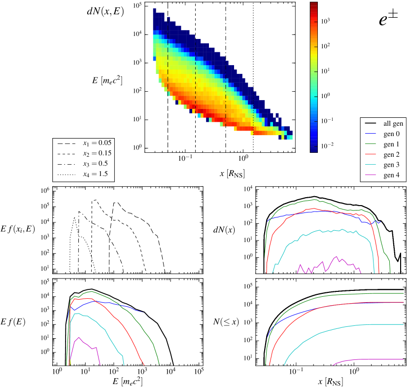
Figure 15.— Cascade portrait of electron-positron pairs. Top panel: number of particles produced in each energy and distance bin $dN(x,E)$ color coded in logarithmic scale according to the colorbar on the right. Middle left: $E\,f(x_{i},E)$ – energy distribution of particles produced at four distances $x_{i},i=1\dots 4$; different line styles correspond to different distances according to the left plot legend. Bottom left: $E\,f(E)$ – energy distribution of all particles produced in the cascade. Middle right: $dN(x)$ – differential pair production rate – number of particles produced in a distance bin. Bottom right: $N(\leq{}x)$ – total number of particles produced up to the distance $x$. Color lines in plots for $E\,f(E)$, $dN(x)$, and $N(\leq{}x)$ show contributions of different cascade generations, lines are color-coded according to the right plot legend. Thick black lines show contributions of all cascade generations. $x$ is the distance from the NS normalized to NS radius $R_{\textrm{\scriptsize{{ns}}}}$ and $E$ is particle energy normalized to $m_{e}c^{2}$. Particle number density is normalized to $n_{\textrm{\scriptsize{{gj}}}}$. Parameters of this simulation: pulsar period $P=33$ ms; the magnetic field in the PC has $B_{0}=10^{12}$ G and $\rho_{\textrm{\scriptsize{c}}}=\mbox{$8.8\times 10^{6}$}$ cm; initial energy of primary particles $\epsilon_{\pm}^{0}=\mbox{$2.3\times 10^{7}$}$.

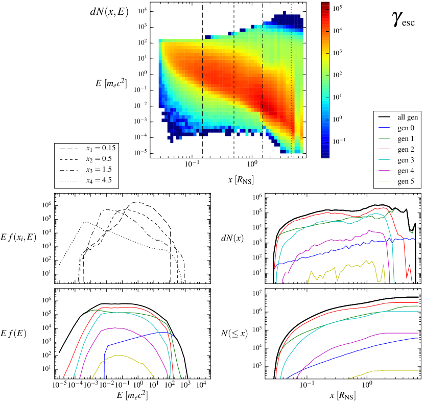
Figure 16.— Cascade portrait of escaping photons for the same cascade as in Fig. 15. Notations and normalizations are the same as in Fig. 15.

In Figures 15 and 16 we show a set of five plots which we call “cascade portraits”. These plots illustrate different aspects of the cascade development by showing moments of the photon or particle distribution function $f(x,E)$. The top panel shows the number of particles produced in each energy and distance bin

$$dN(x,E)=f(x,E)\,dx\,dE,$$ (43)

as a 2D color map. The number of particles is color coded in logarithmic scale according to the color bar on the right. The middle left plot shows the energy distribution $E\,f(x_{i},E)$ of particles produced at four distances $x_{i},i=1\dots 4$; different line styles correspond to different distances according to the left plot legend. These spectra are essentially cross-sections of the map of $dN(x,E)$ (multiplied by particle energy) along four lines shown in the plot for $dN(x,E)$. The bottom left plot shows the energy distribution of all particles produced in the cascade ($dN(x,E)$ integrated along $x$ direction and multiplied by $E$)

$$E\,f(E)=E\int_{0}^{x_{\max}}d\tilde{x}\,f(\tilde{x},E)\,.$$ (44)

In this and the following plots, colored lines show contributions of different cascade generations; lines are color-coded according to the right plot legend. The middle right plot shows the differential pair production rate – number of particles produced in a distance bin ($dN(x,E)$ integrated along the $E$ direction)

$$dN(x)=dx\,\int_{0}^{E_{\max}}f(x,E)\,dE\,.$$ (45)

The bottom right plot shows the cumulative pair production rate – total number of particles produced up to the distance $x$

$$N(\leq{}x)=\int_{0}^{x}d\tilde{x}\,\int_{0}^{E_{\max}}f(\tilde{x},E)\,dE\,.$$ (46)

Figure 15 shows the cascade portrait of the pairs (we do not differentiate between electrons and positrons). The cascade extends to about $\sim 6R_{\textrm{\scriptsize{{ns}}}}$, where it dies out completely as the magnetic field strength and the accelerated particle energy decrease. The pair number grows very quickly, within a few tenths of a NS radius, and then saturates at $\kappa\approx\mbox{$7.4\times 10^{4}$}$. The majority of pairs are produced at distances $<R_{\textrm{\scriptsize{{ns}}}}$ (see plot for $N(\leq{}x)$), which supports the assumption about the length of the cascade zone being $\sim R_{\textrm{\scriptsize{{ns}}}}$ made in § 3.1. The number of pair generations is highest at $\lesssim R_{\textrm{\scriptsize{{ns}}}}$, up to six in this case. The occurrence of most of the cascade generations at distances up to $\sim R_{\textrm{\scriptsize{{ns}}}}$ is the evidence that the photon mfp in a strong cascade is indeed small, $l_{\gamma}\ll R_{\textrm{\scriptsize{{ns}}}}$, so that the cascade initiated by any given particle goes through several generations within the distance $\sim R_{\textrm{\scriptsize{{ns}}}}$. The large extent of the cascade zone relative to $l_{\gamma}$ is due to continuous injection of pair-producing CR photons (see the blue line in the plot of $dN(x)$; generation 0 pairs are produced by CR photons). The largest contribution to pair multiplicity in this case comes from generation 1, pairs created by the first synchrotron photons (see plots for $dN(x)$ and $N(\leq{}x)$). In our simulations for different pulsar parameters, contributions of generation 1 and 2 to the pair multiplicity sometimes become comparable; for weaker cascades the relative contribution of generation 0 is higher than in this case, however we did not see generations 3 and higher producing the majority of pairs. The number of cascade generations is not very large in any of our simulations (several at most), but in each generations high numbers of pair producing photons are emitted which results in high multiplicity.

The energy of created pairs decrease with distance (see plots for $dN(x,E)$ and $E\,f(x_{i},E)$), mostly because of energy losses of primary particles which results in lower energy CR photons. The pair spectrum extends down to a few $mc^{2}$, since the cascade is very efficient at converting initial pair energy into more photons (and pairs). Degradation of pair energies through cascade generations discussed in § 4.3 is clearly visible on the plot for $E\,f(E)$ – the maximum pair energy systematically decreases with cascade generations at all distances.

Figure  16 show the portrait of photons escaping the cascade. Photon generation 0 is CR while the higher generations ($\leq 1$) are synchrotron/cyclotron radiation. Although the highest energy photons are produced nearest the NS surface, these photons are absorbed by pair production attenuation so that the spectra at the lowest altitudes show sharp cutoffs near $100~{}mc^{2}$. This cutoff is clearly visible in the plot for $Ef(x_{i},E)$ for $x_{1}=0.15R_{\textrm{\scriptsize{{ns}}}}$ shown by a dashed line. In the plot for $dN(x,E)$ the cutoff is evident as a sharp horizontal boundary of the colored region for $x\lesssim 0.16R_{\textrm{\scriptsize{{ns}}}}$. The escaping photon energies increase with distance from the NS surface, as the magnetosphere becomes more transparent. The highest escaping photon energies are produced near the end of the cascade, at around 4 NS radii. The highest energy photons escaping the cascade are CR photons (blue line in the plot for $Ef(E)$). Synchrotron radiation is emitted by pairs right after their creation, so that the pair formation and synchrotron radiation end at the same distance – in the plot for $dN(x)$, the number of photons in each generation drops at large distances in accordance with the drop of number of injected pairs shown on a similar plot in Fig. 15. Above $\sim 4R_{\textrm{\scriptsize{{ns}}}}$ the emitted CR photon energies drop as the primary particles continue to lose energy. The spectrum of escaping photons also broadens at the lower end because, as the magnetic field decreases, so does the cyclotron energy which sets the lower limit of the synchrotron spectrum. Thus the lowest and the highest energy escaping photons are produced at the largest distances from then NS, cf. spectra at different $x_{i}$ in the plot for $Ef(x_{i},E)$. The bulk of high energy emission from the PC cascade comes from synchrotron radiation of pairs in generations 1,2, and 3.

Quantitatively, our semi-analytic theory compares with this particular numerical simulation as follows. For pulsar parameters used in this simulation, the energy of primary particles according to eq. (41) should be $\epsilon_{\pm}^{0,\,\textrm{\scriptsize{a}}}\approx\mbox{$3.6\times 10^{7}$}$, which is $\approx 1.6$ times larger than the result obtained from numerical simulations with PAMINA code $\epsilon_{\pm}^{0,\,\textrm{\scriptsize{num}}}\approx\mbox{$2.3\times 10^{7}$}$. For the multiplicity of the CR-synchrotron cascade started by primary particles with monochromatic energies $\epsilon_{\pm}^{0,\,\textrm{\scriptsize{num}}}$, the semi-analytic model gives $\kappa_{\textrm{\scriptsize{{cr}-syn}}}^{\textrm{\scriptsize{a}}}\approx\mbox{$1.56\times 10^{5}$}$, from eq. (23), which is also about $2$ times higher than the value obtained in numerical simulations $\kappa^{\textrm{\scriptsize{num}}}\approx\mbox{$7.4\times 10^{4}$}$. The combined model from § 7, which uses the analytic model for particle acceleration as an input for the semi-analytic model of CR-synchrotron cascade, predicts for the multiplicity $\kappa^{\textrm{\scriptsize{a}}}\approx\mbox{$2.9\times 10^{5}$}$, see Fig. 14, which is $\approx 4$ times larger than the multiplicity from numerical simulations. The discrepancy with the semi-analytic model for several other numerical simulations we performed with different parameters is of the same order. We attribute this discrepancy mostly to the approximation of constant magnetic field – in the numerical simulations, where $B$ and $\rho_{\textrm{\scriptsize{c}}}$ (which is derived from $B$) depend on the distance according to eq. (42), photon absorption decreases and becomes less efficient with the distance. We think that for such a simple model the agreement with the numerical simulations is reasonable and the model can be used for estimates of multiplicities in young energetic pulsars.

9. Resonant Inverse Compton Scattering

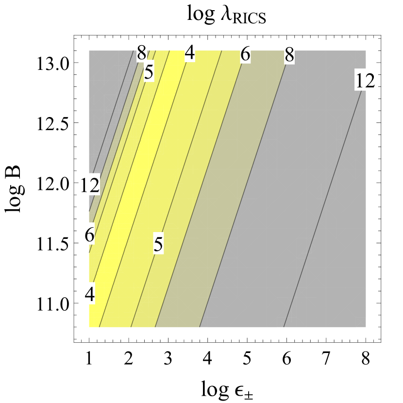
Figure 17.— Distance (in cm) over which a particle loses its energy via resonant inverse Compton scattering. Contours of $\log{\lambda_{\textrm{\scriptsize{RICS}}}}$ are plotted as a function of logarithms of particle energy $\epsilon_{\pm}$ and magnetic field $B$ in Gauss for a NS surface temperature $T=10^{6}$K and $\mu_{s}=0.5$.

Figure 18.— Diagram showing the general chain of physical processes in a strong polar cap cascade. Cascade generations are shown on the left – numbers connected by double arrows. In each generation particles $e^{\pm}$ (electrons and/or positrons) produce photons ($\gamma_{\textrm{\scriptsize{{cr}}}}$ – via curvature radiation, $\gamma_{\textrm{\scriptsize{syn}}}$ – via synchrotron radiation, $\gamma_{\textrm{\scriptsize{RICS}}}$ – via Resonant inverse Compton scattering), which are turned into pairs of the next cascade generation. The CR-synchrotron cascades studied in detail in this paper are shown by solid arrow, dashed arrows show RICS initiated branches which are discussed only in § 9.

Figure 19.— Ratio of of the characteristic energy of RICS photons $\epsilon_{\gamma,\,\textrm{\scriptsize{{RICS}}}}^{(1)}$ emitted by the first generation pairs to the energy of escaping photons: contours of $\log\left[\epsilon_{\gamma,\,\textrm{\scriptsize{{RICS}}}}^{(1)}/\epsilon_{\gamma,\,\textrm{\scriptsize{esc}}}\right]$ are plotted as a function of of logarithms of the radius of curvature of magnetic field lines $\rho_{\textrm{\scriptsize{c}}}$ in cm and magnetic field strength $B$ in Gauss. We used the following values for gap parameters $P=33$ ms, $\xi_{j}=2$ and $\chi_{a}=1/7$.

Another emission mechanism for relativistic particles besides curvature and synchrotron radiation is inverse Compton scattering (ICS). In strong magnetic fields typical for pulsar polar caps, ICS can occur in the resonant regime, when the photon energy in the electron’s rest frame is equal to the cyclotron energy. The cross-section for scattering of such photons is greatly enhanced compared to that of non-magnetic scattering. It has been noted that resonant ICS (RICS) with the soft thermal photons from the NS surface is important for high-energy emission from pulsar polar caps (Sturner, 1995; Zhang & Harding, 2000) and can be important in the development of polar cap cascades because for quite a wide range of pulsar parameters, scattered photons can be above pair-formation threshold (e.g. Sturner et al., 1995; Zhang & Harding, 2000). In this section we argue that although RICS can play a role in the development of polar cap cascades, it never becomes the dominant source for pair multiplicity and, therefore, considering only CR-synchrotron cascades provides adequate estimates for pair multiplicity in strong cascades of normal pulsars. A detailed study of the role of RICS in polar cap cascades will be presented in a subsequent paper.

First, let us consider the efficiency of RICS in transforming particle kinetic energy into radiation. The distance over which a particle loses most of its energy to RICS is given by (Zhang & Harding, 2000; Sturner, 1995; Dermer, 1990):

$$\lambda_{\textrm{\scriptsize{RICS}}} = -0.061\,\epsilon_{\pm}^{2}\,T_{6}^{-1}B_{12}^{-2}\times$$ (47)

$$\ln^{-1}\left[1-\exp\left(-\frac{134B_{12}}{\epsilon_{\pm}\,T_{6}(1-\mu_{s})}\right)\right]\,\mbox{cm}$$

where $T_{6}$ is the temperature of the NS surface in units of $10^{6}$K, $B_{12}$ is the magnetic field strength in units of $10^{12}$ G, and $\mu_{s}=\cos\theta_{s}$, where $\theta_{s}$ is the angle between the momenta of the scattering photon and particle in the lab frame. If the NS is young, its surface temperature comes mostly from cooling and should be about $10^{6}$K. It emits X-ray photons necessary for RICS from the whole surface, and for particles at a distance comparable to the NS radius the range of $\mu_{s}$ is quite large. For older NS, with full surface temperatures below few$\times 10^{5}$K only the polar cap region, heated by the backflow of accelerated particles up to $\sim\mbox{few}\times{}10^{6}$K (e.g. Harding & Muslimov, 2001, 2002), can emit enough photons for RICS to become important. In the latter case when the particle reaches a distance comparable to the width of the polar cap $r_{\textrm{\scriptsize{pc}}}\simeq 1.4\times 10^{4}\,P$ cm, where $P$ is pulsar period in sec, the range of $\mu_{s}$ gets very small and photons quickly get out of resonance. So, for young NSs RICS is an important radiation process if $\lambda_{\textrm{\scriptsize{RICS}}}\sim R_{\textrm{\scriptsize{{ns}}}}$; for old NSs this condition changes to $\lambda_{\textrm{\scriptsize{RICS}}}\sim r_{\textrm{\scriptsize{pc}}}$

In Fig. 17 we plot $\lambda_{\textrm{\scriptsize{RICS}}}$ as a function of particle energy $\epsilon_{\pm}$ and magnetic field $B$, for $T=10^{6}$K and $\mu_{s}=0.5$. It is evident from this plot that primary particles, with $\epsilon_{\pm}>10^{6}$, lose a negligible amount of their energy via RICS, and curvature radiation is the dominant emission mechanism for generation 0 of strong cascades. For cold NSs, RICS of photons from heated polar caps might be an important emission mechanism only for a very narrow energy range of low energetic particles, in one of the later cascade generation – the parameter space between two $\lambda_{\textrm{\scriptsize{RICS}}}=10^{4}$ contours is rather small – and for most values of $B$ the scattered photons will be below pair formation threshold. Hence, RICS can be completely neglected in strong polar cap cascades of cold NSs. For hot NSs RICS becomes an important emission mechanism for a wide range of moderate particle energies $\epsilon_{\pm}<10^{4}$ – the energy range between contours of $\lambda_{\textrm{\scriptsize{RICS}}}=10^{6}$ in Fig. 17 is quite wide. In the latter case, the diagram for physical processes in a strong polar cap cascade can have the general form shown in Fig. 18, with RICS photons in some cases carrying non-negligible energy starting from cascade generation 1. The extension of the semi-analytical analysis of CR-synchrotron cascade developed in §§3–7 to the whole cascade taking into account multiple cascade branches is not straightforward and we postpone it to future publications. Here we will make rough estimates of the contribution of RICS cascade branches to the multiplicity of the whole cascade.

Let us now discuss the efficiency of RICS cascade branches in splitting the available energy into pairs. The energy of photons after scattering by particles of energy $\epsilon_{\pm}$ in the RICS regime is (e.g. Zhang & Harding, 2000)

$$\epsilon_{\gamma,\,\textrm{\scriptsize{{RICS}}}}=2\epsilon_{\pm,\,\textrm{\scriptsize{{f}}}}\,b\,,$$ (48)

where $\epsilon_{\pm,\,\textrm{\scriptsize{{f}}}}$, given by eq. (12), is the kinetic energy of a particle moving along a magnetic field line – the final energy of freshly created pairs after they emit all perpendicular to $B$ energy via synchrotron radiation. Using eqs. (48), (12) together with eq. (21) for the energy of CR photons and eq. (41) for the energy of the primary particle, we get an upper limit on the energy of the generation 1 RICS photons – the highest energy RICS photons. In Fig. 19 we plot the ratio of the energy of generation 1 RICS photons $\epsilon_{\gamma,\,\textrm{\scriptsize{{RICS}}}}^{(1)}$ to the energy of photons escaping from the cascade zone $\epsilon_{\textrm{\scriptsize{esc}}}$ as a function of the radius of curvature of magnetic field lines and the strength of the magnetic field $B$. It is easy to see that for magnetic fields weaker than a few $\times 10^{11}$ G, even the highest energy RICS photons are not capable of producing electron-positron pairs. For stronger magnetic fields, however, RICS photons do contribute to pair multiplicity.

The characteristic energy of RICS photons in terms of the energy of the previous generation photon can be obtained by substituting $\epsilon_{\pm,\,\textrm{\scriptsize{{f}}}}$ into eq. (48)

$$\epsilon_{\gamma,\,\textrm{\scriptsize{{RICS}}}}^{(i+1)}=\epsilon_{\gamma}^{i}\,b\left[1+\left(\frac{\chi_{a}}{b}\right)^{2}\right]^{-1/2}\,.$$ (49)

This equation describes the energy degradation in each cascade generation for the RICS process. In Fig. 20 we plot the ratio of the characteristic energies of synchrotron and RICS photons (given by eqs. (49) and (16) correspondingly) produced by pairs created by the same parent photon as a function of the parent photon energy $\epsilon_{\gamma}^{(i)}$ and magnetic field strength $B$. The energy of RICS photons are always smaller than the energy of synchrotron photons, and for $B<10^{12}$ G significantly so. Because of the much faster energy degradation in the RICS process, cascade branches initiated by RICS photons are in general shorter than those initiated by synchrotron photons. In later cascade generations RICS photons freely escape the cascade zone while synchrotron photons emitted by the same particles are absorbed, still splitting the energy of the parent photons into pairs. Therefore, RICS cascade branches should be in general less efficient in splitting the energy than synchrotron ones.

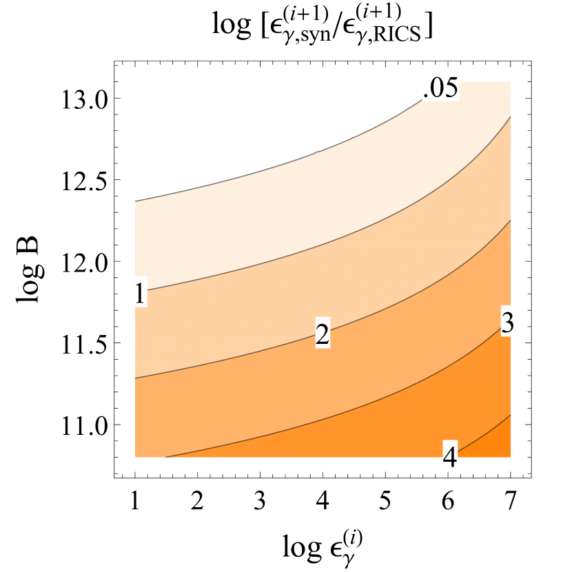
Figure 20.— Ratio of the characteristic energies of synchrotron $\epsilon_{\gamma,\,\textrm{\scriptsize{syn}}}^{(i+1)}$ and RICS $\epsilon_{\gamma,\,\textrm{\scriptsize{{RICS}}}}^{(i+1)}$ photons emitted by freshly created pairs ($(i+1)^{th}$ generation cascade photons): contours of $\log\left[\epsilon_{\gamma,\,\textrm{\scriptsize{syn}}}^{(i+1)}/\epsilon_{\gamma,\,\textrm{\scriptsize{{RICS}}}}^{(i+1)}\right]$ are plotted as a function of logarithms of the parent photon energy $\epsilon_{\gamma}^{(i)}$ and magnetic field strength $B$ in Gauss for $\rho_{\textrm{\scriptsize{c}}}=10^{7}\mbox{cm}$.

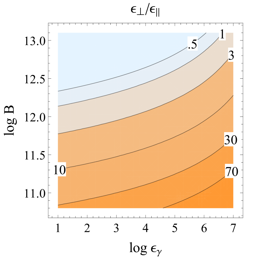
Figure 21.— Ratio of perpendicular to parallel to $B$ energy of freshly created pairs: contours of $\epsilon_{\perp}/\epsilon_{\parallel}$ as a function of logarithms of the parent photon energy $\epsilon_{\gamma}$ and magnetic field strength $B$ in Gauss for $\rho_{\textrm{\scriptsize{c}}}=10^{7}\mbox{cm}$.

Finally let us address the question of how much energy is going into RICS branches of the cascade. The energy powering RICS branches is the kinetic energy of pairs moving along magnetic field lines, while synchrotron branches are powered by the perpendicular energy of freshly created pairs. From eqs. (12), (13) we get for the ratio of the perpendicular to parallel pair energies

$$\frac{\epsilon_{\perp}}{\epsilon_{\parallel}}=\left[1+\left(\frac{\chi_{a}}{b}\right)^{2}\right]^{-1/2}-1\,.$$ (50)

As $\chi_{a}>b$ (see eq. (8)), the minimum value for this ratio is $\sqrt{2}-1\simeq 0.414$. In Fig. 21 we plot $\epsilon_{\perp}/\epsilon_{\parallel}$ as a function of the energy of the parent photon and magnetic field strength $B$. For most of the parameter space in each pair creation event, the fraction of energy going into a the RICS cascade branch is smaller than those going into the synchrotron branch. Even in the case when more energy is left in the pairs’ parallel motion, the energy available to the RICS branch is only $1.5$ times larger than the energy available for synchrotron branch. In this case, however, the value of $\chi_{a}$ is close to $b$, i.e. pair formation occurs near the kinematic threshold and is not very efficient (see § 3.1). Hence, cascades where RICS branches have more available energy should not be very efficient.

Summarizing the above arguments, RICS branches are less efficient in splitting photon energy into pairs and the energy available to those branches is in the best case comparable to the energy available for synchrotron branches. The effect of RICS branches are strongest for higher values of the magnetic field, $\gtrsim\mbox{few}\times 10^{12}$ G, when pair formation happens close to kinematic threshold and the cascade multiplicities are lower than for weaker magnetic fields. The final multiplicity of the total cascades should be less than twice that of the pure CR-synchrotron cascade in the best case and so the pure CR-synchrotron cascades studied in this paper provide good estimates for the multiplicity of strong polar cap cascades.

10. Flux of primary particles and pair yield

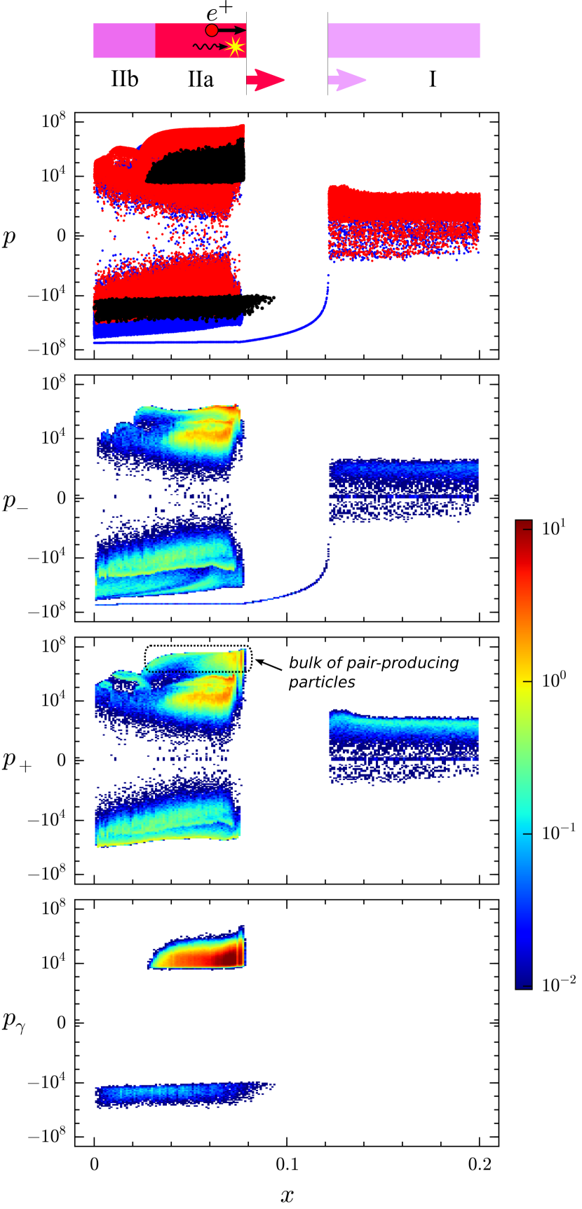
Figure 22.— Snapshot of the phase space for Ruderman-Sutherland cascade at the end of a discharge. Cascade an pulsar parameters: $j_{\textrm{\scriptsize{m}}}/j_{\textrm{\scriptsize{{gj}}}}=1$ $B=10^{12}$ G, $P=33$ ms, $\xi_{j}=1$. Horizontal axis – particle positron $x$, vertical axis – particle momentum normalized to $m_{e}c$; the vertical axis is logarithmic except for the region around zero momentum ($-5<p<5$), where the scale is linear. The top panel shows phase space portrait of the cascade: each dot represents a numerical particle (every 10th particle is plotted); blue dots – electrons, red dots – positrons, black dots – photons. Three plots beneath show particle number density in phase space: $p_{-}$ vs $x$ – electrons, $p_{+}$ vs $x$ – positrons, $p_{\gamma}$ vs $x$ – photons. Particle number density is color-coded according to the color map on the right in units of $n_{\textrm{\scriptsize{{gj}}}}$. Particles which produce most of the pairs are positrons inside the area surrounded by dotted line marked as “bulk of pair-producing particles”. On the top of the plots we show the sketch of the structure of the acceleration zone from Fig. 11(b).

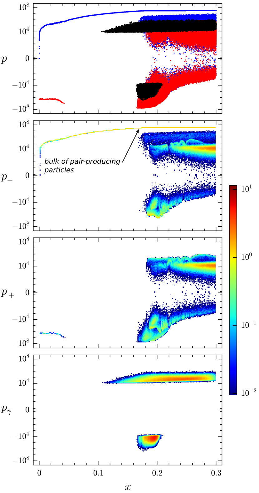
Figure 23.— Snapshot of the phase space for cascade in Space Charge Limited Flow regime. Cascade an pulsar parameters: $j_{\textrm{\scriptsize{m}}}/j_{\textrm{\scriptsize{{gj}}}}=1.5$ $B=10^{12}$ G, $P=33$ ms, $\xi_{j}=0.25$. Types of plots and notations are the same as in Fig. 22.

As we have shown above, for the most efficient polar cap cascades the total pair yield for a given value of the magnetic field $B$ depends mostly on the flux of primary particles. According to self-consistent models of polar cap acceleration zones (T10, TA13), particle acceleration is intermittent and the pattern of plasma flow and acceleration efficiency depends on the ratio of the current density imposed by the magnetosphere to the GJ current density $j_{\textrm{\scriptsize{m}}}/j_{\textrm{\scriptsize{{gj}}}}$ as well as the boundary conditions at the NS surface – whether particles can be extracted from the surface or not.

There are essentially three qualitatively different regimes of plasma flow that determine the flux of primary pair-producing particles: (i) in space charge limited flow with $0<j_{\textrm{\scriptsize{m}}}/j_{\textrm{\scriptsize{{gj}}}}<1$ particles are accelerated up to very low energies, $\epsilon_{\pm}\sim$ few, and no pairs are produced, (ii) in space charge limited flow with $j_{\textrm{\scriptsize{m}}}/j_{\textrm{\scriptsize{{gj}}}}>1$ a significant flux of primary particles of the order of $\sim j_{\textrm{\scriptsize{{gj}}}}/e$ is accelerated through the gap while the gap is moving toward the NS, (iii) in all other cases – i.e. for any current density in Ruderman-Sutherland model and for $j_{\textrm{\scriptsize{m}}}/j_{\textrm{\scriptsize{{gj}}}}<0$ in space charge limited flow regime – in each burst of pair formation a blob of primary particles is produced during formation of the gap, and then no significant amount of primary particles is created until the formation of the next gap.

In Fig. 22 we plot as an example for case (iii) a phase portrait and densities of plasma and photons in the phase space for a Ruderman-Sutherland cascade with $j_{\textrm{\scriptsize{m}}}/j_{\textrm{\scriptsize{{gj}}}}=1$. The process of gap formation for this case is described at the beginning of §6.2. When the gap is formed, only a very few particles leak from the plasma tail – in this case electrons, visible as a line-like feature in the top two panels of Fig. 22 – are accelerated in the gap, the flux of these particles is much less than $\sim j_{\textrm{\scriptsize{{gj}}}}/e$ and their contribution to the pair production can be neglected. The blob of primary particles which was created during the gap formation has a density of a few $n_{\textrm{\scriptsize{{gj}}}}$ in its densest parts and a size comparable to the gap’s height. Those particles – in this case positrons in the area surrounded by a dotted line on the plot for positron phase space density in Fig. 22 – create the vast majority of pairs. The density of primary particles in the blob is high but no new primary particles are created until the next gap is formed, the duty cycle of the cascade is small. The resulting flux of primary particles averaged over the period of gap formation is rather low.

In case (ii), in space-charge limited flow with super GJ current density, the situation is qualitatively different in that during the lifetime of the gap, and not only during the time the gap is forming, as in case (iii), a significant constant flux of particles is going through the acceleration zone. The duty cycle of such a cascade should be substantially higher than in any other types of cascades. As an example of such a cascade we plot in Fig. 23 a phase portrait and the densities of plasma and photons in phase space for a cascade in space-charge limited flow regime with $j_{\textrm{\scriptsize{m}}}/j_{\textrm{\scriptsize{{gj}}}}=1.5$. The gap is formed at some distance from the NS and moves toward it. When the first particles are formed the process of electric field screening proceeds in a similar way to the case of Ruderman-Sutherland cascades; the blob of ultrarelativistic particles is created and particles leaking from it create a tail of mildly relativistic plasma screening the electric field behind the blob; this blog moves toward the NS creating pairs. However a constant flux of particles extracted from the NS surface – in this case electrons, visible as a line-like feature in the top two panels of Fig. 23 – are accelerated in the gap. The density of these electrons is high (for the case shown in Fig. 23 it is $\simeq 1.25\,n_{\textrm{\scriptsize{{gj}}}}$) and these particles, and not the particles from the blob, produce most of the pairs.

Because of the intermittency of pair formation, the resulting multiplicity must be adjusted by the relative fraction of time during which primary particles are produced. If $\tau_{\textrm{\scriptsize{active}}}$ is the time of active particle acceleration and $T_{\textrm{\scriptsize{cascade}}}$ is the time between the beginning of successive bursts of pair creation, then the pair multiplicity as discussed in previous sections should be multiplied by the attenuation factor

$$f_{\kappa}=\frac{\tau_{\textrm{\scriptsize{active}}}}{T_{\textrm{\scriptsize{cascade}}}}$$ (51)

to get the average multiplicity of pair cascades.

The existing self-consistent simulations of particle acceleration (T10, TA13) are inconclusive about the cascade repetition rate. The numerical resolution in these simulations was inadequate for that purpose – because of copious pair formation the Debye length of plasma at some point became smaller than the cell size and the formation of the plasma tail could not be simulated accurately; the repetition rate, however, is determined by the mildly relativistic plasma in the plasma tail, as the next burst of pair formation starts only when plasma leaves the polar cap region. Future numerical simulations would address this issue and provide accurate values for cascade duty cycles; meanwhile here we will try to give a rough estimate for the cascade repetition rate using the following simple physical arguments.

The strongest pair formation can continue up to the distance of the order of a few NS radii $R_{\textrm{\scriptsize{{ns}}}}$. Although the exact physical mechanism responsible for formation of the mildly relativistic plasma tail is not clear (see previous paragraph) it seems to us plausible to expect that when plasma injection due to pair formation stops, reversal of some pairs toward the NS – plasma leakage from the blob to the tail – should taper off as well. So, the time when plasma is filling the polar cap region is of the order of $\sim R_{\textrm{\scriptsize{{ns}}}}/c$. The mildly relativistic pairs which fill the polar cap region after the blob of plasma has moved away are moving with relativistic velocities, so the time the plasma needs to clear out is also of the order of $\sim R_{\textrm{\scriptsize{{ns}}}}/c$. Therefore, the cascade repetition rate seems to be $T_{cascade}\sim\mbox{few}\times R_{\textrm{\scriptsize{{ns}}}}/c$

For the case (iii), in the flow regime with vacuum gaps – Ruderman-Sutherland cascades or space-charge limited flow in return current regions – particles are accelerated only during formation of the gap, the time of active particle acceleration is quite short. The longitudinal size of the blob of primary particles is about the size of the gap $h_{\textrm{\scriptsize{gap}}}$, and the primary particle density in the blob is a few $n_{\textrm{\scriptsize{{gj}}}}$. All primary particles in the blob move in the same direction and the blob passes any given surface normal to the field lines during time $\tau_{\textrm{\scriptsize{active}}}\sim{}h_{\textrm{\scriptsize{gap}}}/c$. If the next gap will form after the blob of primary particles moves a few $R_{\textrm{\scriptsize{{ns}}}}$ away, the attenuation factor should be

$$f_{\kappa}\sim\frac{h_{\textrm{\scriptsize{gap}}}}{R_{\textrm{\scriptsize{{ns}}}}}\simeq\mbox{$4\times 10^{-2}$}\>\chi_{a}^{1/7}\xi_{j}^{-3/7}\rho_{\textrm{\scriptsize{c,\,7}}}^{2/7}P^{3/7}B_{12}^{-4/7}$$ (52)

For the Crab pulsar this attenuation factor is around $0.001$ if we assume $P=33$ ms, $B=\mbox{$3\times 10^{12}$}$ G, $\chi_{a}=1/7$, and $\xi_{j}=1$ (for inclination angle $60^{\circ}$ and current density $j_{\textrm{\scriptsize{m}}}\simeq j_{\textrm{\scriptsize{{gj}}}}$). The resulting multiplicity of such cascades in Crab would be $\lesssim{}10^{3}n_{\textrm{\scriptsize{{gj}}}}$.

In the space-charge limited flow regime with super-GJ current density, case (ii), the cascade efficiency should be much higher. The gap appears at some distance and moves toward the NS (see § 6.2 in TA13). The process of gap formation is very similar to that in cascades for case (iii) discussed above. A blob of relativistic particles is created, which in this case propagates toward the NS, and pair plasma leaking from it creates a plasma tail filling the region behind the blob which prevents formation of the next gap. But in this case particles extracted from the NS surface flow into the magnetosphere through the gap and are accelerated all the time the gap exists; these particles create most of the pairs. When the gap disappears, particle acceleration stops. The remaining plasma should leave the gap and flow into the magnetosphere before the next gap can appear. The time necessary for the remaining plasma to leave should be comparable to the time of the gap’s existence, as all particles are relativistic. Therefore, in this case the attenuation factor should be $f_{\kappa}\sim{}1/\mbox{few}$ – much higher than given by eq. (52). So, polar cap regions with super-GJ current density should have a pair yield of about $10^{5}n_{\textrm{\scriptsize{{gj}}}}$.

Let us summarize our findings. Pulsars with polar cap cascades operating in the Ruderman-Sutherland regime would not be efficient pair producer, the highest yield should be less that $\sim{}10^{3}n_{\textrm{\scriptsize{{gj}}}}$. If the polar cap cascades operate in the space charge limited flow regime, then in regions with super-GJ current densities the pair yield is quite high, around $10^{5}n_{\textrm{\scriptsize{{gj}}}}$; in the regions with return current (anti-GJ current density) the yield should be less that $\sim{}10^{3}n_{\textrm{\scriptsize{{gj}}}}$, and in regions with sub-GJ current densities no pair plasma would be produced at all. We therefore conclude that the maximum pair yield of a young pulsar would be less that $10^{5}n_{\textrm{\scriptsize{{gj}}}}$, as only a fraction of the polar cap can have super-GJ current density.

Pair yield is mostly affected by the duty cycle of the cascade, and not by pulsar parameters such as magnetic field strength $B$, radius of curvature of magnetic field lines $\rho_{\textrm{\scriptsize{c}}}$, or pulsar period $P$. This holds only for the regime in which the gap height is much smaller than the PC radius, true for all young pulsars. When the gap height approaches and exceeds the PC radius, the pair yield drops quickly, as shown in Figure 9. The distribution of $j_{\textrm{\scriptsize{m}}}/j_{\textrm{\scriptsize{{gj}}}}$ in the polar cap is determined by the pulsar inclination angle and we expect that inclination angle should be the most important factor determining pair yield of a young pulsar.

11. Discussion

We have performed a systematic study of electron-positron pair cascades above pulsar polar caps for a variety of input parameters including surface magnetic field, pulsar rotation period, primary particle energy and magnetic field radius of curvature. We have also studied here for the first time the multiplicity of self-consistent pair cascades, i.e. those that are capable of generating currents consistent with global magnetosphere models.

We find that pair multiplicity is maximized for a magnetic field strength near $10^{12}$ G, independent of the other parameters. This value of field strength strikes a balance between maximizing the fraction of photons that pair produce – the weaker the magnetic field the higher the number of escaping photons – and the fraction of photon energy going into pair production – in stronger fields photons are absorbed when they have smaller angles to $B$, and created pairs, having smaller perpendicular to $B$ momenta, emit less synchrotron photons, which produce the next generation of pairs. This is true for curvature radiation - synchrotron cascades, which should be the dominant source of pairs in young energetic pulsars. For stronger magnetic fields $B\gtrsim\mbox{$3\times 10^{12}$}$ G resonant inverse Compton scattering of soft X-ray photons emitted by the NS surface can tap some of the pair’s energy parallel to $B$ and increase the cascade multiplicity. RICS cascade branches, however, are less efficient than the synchrotron branches; this together with the decrease of the photon absorption cross-section for near threshold pair creation in strong magnetic fields should not change the fact the polar cap cascade multiplicity reaches its maximum for $B\sim 10^{12}$ G.

We find that the pair multiplicity at the peak of the cascade cycle, $\kappa\sim 10^{5}$, is remarkably insensitive to pulsar period, magnetic field and radius of curvature of magnetic field lines. The reason for this is self-regulation of the accelerator by pair creation: for pulsar parameters resulting in more efficient pair production, the size of the acceleration gap is smaller and the primary particle energy is lower and vice-versa. The most important factor determining the multiplicity of polar cap cascades is the flux of primary particles which depends on the “duty cycle” of the particle acceleration in time-dependent cascades. Estimating the “duty cycle” we find that the time-averaged pair multiplicity is limited to $\sim 10^{5}$ for the case of space charge-limited flow (free particle extraction from the NS) with super Goldreich-Julian current density ($j/j_{\textrm{\scriptsize{{gj}}}}>1$) and to only $\sim 10^{3}$ for the case of Ruderman-Sutherland gaps (no particle extraction from the PC) and space charge-limited flow with anti Goldreich-Julian current density ($j/j_{\textrm{\scriptsize{{gj}}}}<0$). The current density distribution in the PC depends on the pulsar inclination angle, and so for young energetic pulsars the inclination angle should be the most important factor determining the total multiplicity of plasma in the magnetosphere.

Our finding of a peak multiplicity from self-consistent pair cascades in young pulsars ($\sim 10^{5}$), that is largely independent of their period and magnetic fields, is very different from previous predictions from steady cascades that produce a range of multiplicities ($10^{2}-10^{4}$) that depend strongly on pulsar parameters. This difference primarily results from much smaller gap heights in the time-dependent cascades, that keep the gap size much less than the PC radius over a large parameter range. This in turn results in a nearly uniform magnetic field strength throughout the gaps, higher accelerating electric fields, higher primary particle energies and more efficient pair production – primary particles are accelerated faster and photons are injected in the region of stronger magnetic field than in previous steady cascade models.

We have also numerically simulated the photon spectra from self-consistent polar cap pair cascades. Our results show that the cascade photon spectra from the more compact gaps nearer to the neutron star surface have cutoffs that are around 10 - 100 MeV. This is at the lower end the Fermi energy band ($30$ MeV - $300$ GeV), which may explain why Fermi has not seen strong evidence for $\gamma$-ray emission from the PC. High energy emission from pair cascades is thus expected to occur in lower energy bands, below 100 MeV. PC cascade emission may have been detected recently from PSR J1813-1246 (Marelli et al., 2014) at X-ray energies by XMM-Newton and Chandra. The unusual X-ray light curve that shows two peaks separated by 0.5 in phase but offset by a quarter of a period with the $\gamma$-ray peaks can be explained through a geometric model placing the $\gamma$-ray emission in the outer magnetosphere and the X-ray emission at lower altitude above the PCs, and could be coming from the PC cascades.

Our results show that PC cascades are more efficient in producing electron-positron pairs that was previously assumed. However, even the higher pair multiplicity of $10^{5}$ is not enough to account for the fluxes of particles needed to explain the synchrotron radiation from PWNe. Based on a multiplicity of $10^{5}$, we estimate that the Crab pulsar produces a pair flux from each PC of about $\mbox{$2\times 10^{39}$}\,\mbox{pairs}\,\mbox{s}^{-1}$. The flux from both PCs is an order of magnitude smaller than the pair flux required to account for the radiation from the nebula, which is estimated to be about $\sim\mbox{$4\times 10^{40}$}\,\mbox{pairs}\,\mbox{s}^{-1}$ (de Jager et al., 1996). Cascades in the outer magnetosphere are not very efficient pair producers (e.g. Hirotani, 2006), and so the injection of plasma by pulsars can not account for the population of particles in PWNe emitting at radio wavelengths. These radio emitting particles must then have a different origin from particles emitting at shorter wavelength; for example, they might be picked up from the gas filaments in the supernova remnant or be remnants of some unknown acceleration mechanism in the early history of the nebula (Atoyan & Aharonian, 1996).

Another implication of our results concerns observations of cosmic-ray electrons and positrons at Earth that have shown an excess of positrons over what can be produced in secondary cosmic-ray interactions (Adriani et al., 2009; Accardo et al., 2014), indicating the existence of primary positron sources in the Galaxy. Various studies (e.g. Gendelev et al., 2010) have estimated that PWNe could account for the excess of cosmic ray positrons. With higher pair multiplicity from young pulsars, and subsequent acceleration of the pairs at the pulsar wind termination shock, PWNe could produce a more significant contribution of primary cosmic ray positrons.

Appendix A Algorithms for semi-analytical calculation of cascade multiplicity

Here we show pseudo-codes of algorithms used to compute cascade multiplicity. For calculation of $\chi_{a}(\epsilon_{\gamma},B,\rho_{\textrm{\scriptsize{c}}})$ we computed and stored a table of $1/\chi_{a}$ values for a uniformly divided grid $77\times 30\times 20$ in $\log\epsilon_{\gamma}\times\log{B}\times\log{\rho_{\textrm{\scriptsize{c}}}}$ space, and then used cubic piece-polynomial interpolation to get $\chi_{a}$ for parameter values required by expressions used in the algorithms.

Algorithm 1 computes total number of particles produced in synchrotron cascade initiated by a single primary photon with the energy $\epsilon_{\gamma}$, physical processes are described in §4.3. e_phot and n_phot are the number and the energy of synchrotron photons emitted by particles of the current generation, e_phot is the energy of escaping photons, and n is the total number of particles produced in all previous generations.

Data: $\epsilon_{\gamma}$ – energy of primary photon, $s_{\textrm{\scriptsize{esc}}}$ – mfp of escaping photon

Result: $N_{\textrm{\scriptsize{syn}}}$ – total number of particles produced in synchrotron cascade initiated by a photon with the energy $\epsilon_{\gamma}$

Function $N_{\textrm{\scriptsize{syn}}}$($\epsilon_{\gamma},s_{\textrm{\scriptsize{esc}}}$):

       $\textnormal{{e\_esc}}\leftarrow\epsilon_{\gamma,\,\textrm{\scriptsize{esc}}}(s_{\textrm{\scriptsize{esc}}})$

        // eq. (10)

       $\textnormal{{e\_phot}}\leftarrow\epsilon_{\gamma}$

       $\textnormal{{n\_phot}}\leftarrow 1$

       $\textnormal{{n}}\leftarrow 0$

       while e_phot $\geq\textnormal{{e\_esc}}$ do

             $\textnormal{{n}}\leftarrow\textnormal{{n}}+2~{}\textnormal{{n\_phot}}$

             $\textnormal{{n\_phot}}\leftarrow\textnormal{{n\_phot}}~{}n_{\textrm{\scriptsize{syn}}}(\textnormal{{e\_phot}})$

              // eq. (15)

             $\textnormal{{e\_phot}}\leftarrow\epsilon_{\gamma}^{(i+1)}(\textnormal{{e\_phot}})$

              // eq. (16)

            

       end while

       return n

end

Algorithm 1 Multiplicity of synchrotron cascade

Algorithm 2 computes the total multiplicity $\kappa$ of a CR-synchrotron cascade according to eq. (23). e_part is the energy of the primary particle at the current distance $s_{i}$; e_phot is the energy and n_phot is the number of CR photons emitted by the primary particle at the current distance, Nsyn is the number of particles generated in synchrotron cascades initiated by the primary particle at the current distance. Integration over the distance is done with the simple trapezoidal rule.

Data: $\epsilon_{\pm}^{0}$ – energy of the primary particle, $s_{\textrm{\scriptsize{{cr}}}}$ – characteristic size of the cascade, $s_{\textrm{\scriptsize{esc}}}$ – mfp of escaping photons

Result: total number of pairs produced by the primary particle with the energy $\epsilon_{\pm}^{0}$

begin

       divide $[0,s_{\textrm{\scriptsize{{cr}}}}]$ in subintervals $s_{0},\dots{},s_{i_{max}}$

       $\textnormal{{Nsyn\_last}}\leftarrow{0}$

       $\textnormal{{n}}\leftarrow{0}$

      

      for $i\leftarrow 1$ to $i_{max}$ do

             // CR radiation at distance $s_{i}$

             $\textnormal{{e\_part}}\leftarrow\epsilon_{\pm}(\epsilon^{0}_{\pm},\textnormal{{$s_{i}$}})$

              // eq. (19)

             $\textnormal{{e\_phot}}\leftarrow\epsilon_{\gamma,\,\textrm{\scriptsize{{cr}}}}(\textnormal{{e\_part}})$

              // eq. (21)

             $\textnormal{{n\_phot}}\leftarrow n_{\textrm{\scriptsize{{cr}}}}(\textnormal{{e\_part}})$

              // eq. (22)

            

            // synchrotron cascade multiplicity

             $\textnormal{{Nsyn}}\leftarrow\textnormal{{n\_phot}}$ $N_{\textrm{\scriptsize{syn}}}$(e_phot, $s_{\textrm{\scriptsize{esc}}}$)

              // algorithm 1

            

            // trapezoidal rule

             $\textnormal{{n}}\leftarrow\textnormal{{n}}+0.5(\textnormal{{Nsyn}}+\textnormal{{Nsyn\_last}})(\textnormal{{$s_{i}$}}-\textnormal{{$s_{i-1}$}})$

             Nsyn_last $\leftarrow$ Nsyn

            

       end for

       return n

end

Algorithm 2 Multiplicity of CR-synchrotron cascade

Appendix B Transition to radiation reaction limited regime

Radiation reaction begins playing an important role in the dynamics of particle acceleration if particle energy losses per unit time become comparable to the work done on the particle by the accelerating electric field. For curvature radiation the condition for applicability of the free acceleration regime is (see eq. (17))

$$eEc\gtrsim\frac{2}{3}\frac{e^{2}}{c^{3}}\left(\frac{c^{2}}{\rho_{\textrm{\scriptsize{c}}}}\right)^{2}\epsilon_{\pm}^{4}\,.$$ (B1)

The electric field $E$ grows linearly with the distance $l_{\pm}$ traveled by the particle in the gap, eq. (27); the particle energy $\epsilon_{\pm}$ increases as $l_{\pm}^{2}$, eq. (32), and at some distance the condition (B1) is violated. However, if condition (B1) holds up to the distance $l_{\pm}^{\textrm{\scriptsize{e}}}$ where the particle emits “gap-terminating” photons, then the gap length and the final particle energies can be well described by the free acceleration regime, neglecting radiation energy losses. Using eq. (27) for $E$, eq. (32) for $\epsilon_{\pm}$, and substituting $l_{\pm,\,\textrm{\scriptsize{gap}}}^{\textrm{\scriptsize{e}}}$ for $l_{\pm}$ from the eq. (39) inequality (B1) becomes the condition on the magnetic field strength

$$B>\frac{8}{3}\alpha_{f}\chi_{a}B_{q}\simeq\mbox{$2.8\times 10^{-3}$}B_{q}=\mbox{$1.15\times 10^{11}$}\mbox{G}\,.$$ (B2)

In the second step we used the value $\chi_{a}=1/7$. The radius of curvature $\rho_{\textrm{\scriptsize{c}}}$ and pulsar period $P$ cancel out, except for a weak dependence of $\chi_{a}$ on $\rho_{\textrm{\scriptsize{c}}}$. We see that for most non-millisecond pulsars radiation reaction can be neglected.

Appendix C Limit on 1-d approximation

The one-dimensional approximation for particle acceleration in the gaps works well if the length of the gap is much smaller that the width of the polar cap. As the length of the gap is $\sim{}2$ times larger than $l_{\textrm{\scriptsize{gap}}}$, we can set the formal limit on 1-D approximation as

$$l_{\textrm{\scriptsize{gap}}}<r_{\textrm{\scriptsize{pc}}}\,,$$ (C1)

where $r_{\textrm{\scriptsize{pc}}}=\sqrt{2\pi R_{\textrm{\scriptsize{{ns}}}}^{3}/Pc}$ is the polar cap radius. Using eq. (37), (39) for $l_{\textrm{\scriptsize{gap}}}$ and $l_{\pm}^{\textrm{\scriptsize{e}}}$ we get the following limits on pulsar parameters for applicability of the 1-D approximation

$$B^{4/7}P^{-13/14}>\frac{7}{6}\left(\frac{c}{2\pi R_{\textrm{\scriptsize{{ns}}}}^{3}}\right)^{1/2}\left(\chi_{a}\frac{B_{q}^{4}\lambdabar{}_{\textrm{\scriptsize{{c}}}}^{2}c^{3}}{\pi^{3}}\right)^{1/7}\xi_{j}^{-3/7}\,\rho_{\textrm{\scriptsize{c}}}^{2/7}\,.$$ (C2)

The pulsar magnetic field is usually estimated assuming magnetodipolar energy losses from the values of period $P$ and period derivative $\dot{P}$ as $B=\mbox{$3.2\times 10^{19}$}\sqrt{P\dot{P}}$. Expressing $B$ in this way and putting the numerical values for physical constants, we get from eq. (C2) the following condition for applicability of 1-D approximation in terms of $P$ and $\dot{P}$

$$\dot{P}>\mbox{$3.21\times 10^{-22}$}\chi_{a}^{1/2}\xi_{j}^{-3/2}\rho_{\textrm{\scriptsize{c}}}\,P^{9/4}\simeq\mbox{$4.3\times 10^{-16}$}\rho_{\textrm{\scriptsize{c,\,7}}}\,P^{9/4}\,,$$ (C3)

in the last step we used values $\xi_{j}=2$ and $\chi_{a}=1/7$. For cascades along dipole magnetic field lines at the edge of the polar cap with the radius of curvature

$$\rho_{\textrm{\scriptsize{c}}}=\frac{4}{3}\frac{R_{\textrm{\scriptsize{{ns}}}}}{\theta_{\textrm{\scriptsize{pc}}}}\approx{}\mbox{$9.2\times 10^{7}$}\sqrt{P}\,\mbox{cm},$$ (C4)

where $\theta_{\textrm{\scriptsize{pc}}}=\sqrt{2\pi R_{\textrm{\scriptsize{{ns}}}}/cP}$ is the colatitude of the polar cap edge, condition (C3) takes the form

$$\dot{P}>\mbox{$4\times 10^{-16}$}P^{11/4}\,.$$ (C5)

References

- Abdo et al. (2010) Abdo, A. A., Ackermann, M., Ajello, M., et al. 2010, ApJS, 187, 460
- Abdo et al. (2013) Abdo, A. A., Ajello, M., Allafort, A., et al. 2013, ApJS, 208, 17
- Accardo et al. (2014) Accardo, L., Aguilar, M., Aisa, D., et al. 2014, Phys. Rev. Lett., 113, 121101
- Adriani et al. (2009) Adriani, O., Barbarino, G. C., Bazilevskaya, G. A., et al. 2009, Nature, 458, 607
- Arons et al. (2005) Arons, J., Backer, D. C., Spitkovsky, A., & Kaspi, V. M. 2005, in Astronomical Society of the Pacific Conference Series, Vol. 328, Binary Radio Pulsars, ed. F. A. Rasio & I. H. Stairs, 95
- Arons & Scharlemann (1979) Arons, J., & Scharlemann, E. T. 1979, ApJ, 231, 854
- Atoyan & Aharonian (1996) Atoyan, A. M., & Aharonian, F. A. 1996, MNRAS, 278, 525
- Bai & Spitkovsky (2010) Bai, X., & Spitkovsky, A. 2010, ApJ, 715, 1282
- Bucciantini et al. (2011) Bucciantini, N., Arons, J., & Amato, E. 2011, MNRAS, 410, 381
- Cheng et al. (1976) Cheng, A., Ruderman, M., & Sutherland, P. 1976, ApJ, 203, 209
- Contopoulos et al. (1999) Contopoulos, I., Kazanas, D., & Fendt, C. 1999, ApJ, 511, 351
- Daugherty & Harding (1982) Daugherty, J. K., & Harding, A. K. 1982, ApJ, 252, 337
- Daugherty & Harding (1983) —. 1983, ApJ, 273, 761
- de Jager (2007) de Jager, O. C. 2007, ApJ, 658, 1177
- de Jager et al. (1996) de Jager, O. C., Harding, A. K., Michelson, P. F., et al. 1996, ApJ, 457, 253
- Dermer (1990) Dermer, C. D. 1990, ApJ, 360, 197
- Dyks & Harding (2004) Dyks, J., & Harding, A. K. 2004, ApJ, 614, 869
- Erber (1966) Erber, T. 1966, Reviews of Modern Physics, 38, 626
- Gendelev et al. (2010) Gendelev, L., Profumo, S., & Dormody, M. 2010, J. Cosmology Astropart. Phys, 2, 16
- Goldreich & Julian (1969) Goldreich, P., & Julian, W. H. 1969, ApJ, 157, 869
- Gurevich & Istomin (1985) Gurevich, A. V., & Istomin, I. N. 1985, Zhurnal Eksperimental noi i Teoreticheskoi Fiziki, 89, 3
- Harding (1981) Harding, A. K. 1981, ApJ, 245, 267
- Harding et al. (1997) Harding, A. K., Baring, M. G., & Gonthier, P. L. 1997, ApJ, 476, 246
- Harding & Muslimov (2001) Harding, A. K., & Muslimov, A. G. 2001, ApJ, 556, 987
- Harding & Muslimov (2002) —. 2002, ApJ, 568, 862
- Harding & Muslimov (2011) —. 2011, ApJ, 726, L10+
- Harding & Preece (1987) Harding, A. K., & Preece, R. 1987, ApJ, 319, 939
- Hewish et al. (1968) Hewish, A., Bell, S. J., Pilkington, J. D. H., Scott, P. F., & Collins, R. A. 1968, Nature, 217, 709
- Hibschman & Arons (2001a) Hibschman, J. A., & Arons, J. 2001a, ApJ, 554, 624
- Hibschman & Arons (2001b) —. 2001b, ApJ, 560, 871
- Hirotani (2006) Hirotani, K. 2006, ApJ, 652, 1475
- Jackson (1975) Jackson, J. D. 1975, Classical electrodynamics (John Wiley & Sons)
- Kalapotharakos & Contopoulos (2009) Kalapotharakos, C., & Contopoulos, I. 2009, A&A, 496, 495
- Kalapotharakos et al. (2014) Kalapotharakos, C., Harding, A. K., & Kazanas, D. 2014, ApJ, 793, 97
- Lyutikov (2004) Lyutikov, M. 2004, MNRAS, 353, 1095
- Manchester et al. (2005) Manchester, R. N., Hobbs, G. B., Teoh, A., & Hobbs, M. 2005, AJ, 129, 1993
- Marelli et al. (2014) Marelli, M., Harding, A., Pizzocaro, D., et al. 2014, ApJ, 795, 168
- Medin & Lai (2010) Medin, Z., & Lai, D. 2010, MNRAS, 406, 1379
- Pierbattista et al. (2015) Pierbattista, M., Harding, A. K., Grenier, I. A., et al. 2015, A&A, 575, A3
- Ruderman & Sutherland (1975) Ruderman, M. A., & Sutherland, P. G. 1975, ApJ, 196, 51
- Sokolov & Ternov (1968) Sokolov, A., & Ternov, I. 1968, Synchrotron Radiation (Pergamon Press)
- Spitkovsky (2006) Spitkovsky, A. 2006, ApJ, 648, L51
- Sturner (1995) Sturner, S. J. 1995, ApJ, 446, 292
- Sturner et al. (1995) Sturner, S. J., Dermer, C. D., & Michel, F. C. 1995, ApJ, 445, 736
- Sturrock (1971) Sturrock, P. A. 1971, ApJ, 164, 529
- Tademaru (1973) Tademaru, E. 1973, ApJ, 183, 625
- Timokhin (2006) Timokhin, A. N. 2006, MNRAS, 368, 1055
- Timokhin (2010) —. 2010, MNRAS, 408, 2092
- Timokhin & Arons (2013) Timokhin, A. N., & Arons, J. 2013, MNRAS, 429, 20
- Watters et al. (2009) Watters, K. P., Romani, R. W., Weltevrede, P., & Johnston, S. 2009, ApJ, 695, 1289
- Zhang & Harding (2000) Zhang, B., & Harding, A. K. 2000, ApJ, 532, 1150