Spot evolution on the red giant star XX Triangulum

Abstract

Context. Solar spots appear to decay linearly proportional to their size. The decay rate of solar spots is directly related to magnetic diffusivity, which itself is a key quantity for the length of a magnetic-activity cycle. Is a linear spot decay also seen on other stars, and is this in agreement with the large range of solar and stellar activity cycle lengths?

Aims. We investigate the evolution of starspots on the rapidly-rotating ($P_{\rm rot}$ $\approx$ 24 d) K0 giant XX Tri, using consecutive time-series Doppler images. Our aim is to obtain a well-sampled movie of the stellar surface over many years, and thereby detect and quantify a starspot decay law for further comparison with the Sun.

Methods. We obtained continuous high-resolution and phase-resolved spectroscopy with the 1.2-m robotic STELLA telescope on Tenerife over six years, and these observations are ongoing. For each observing season, we obtained between 5 to 7 independent Doppler images, one per stellar rotation, making up a total of 36 maps. All images were reconstructed with our line-profile inversion code iMap. A wavelet analysis was implemented for denoising the line profiles. To quantify starspot area decay and growth, we match the observed images with simplified spot models based on a Monte Carlo approach.

Results. It is shown that the surface of XX Tri is covered with large high-latitude and even polar spots and with occasional small equatorial spots. Just over the course of six years, we see a systematically changing spot distribution with various timescales and morphology, such as spot fragmentation and spot merging as well as spot decay and formation. An average linear decay of $D$ = $-$0.022 $\pm$ 0.002 SH/day is inferred. We found evidence of an active longitude in phase toward the (unseen) companion star. Furthermore, we detect a weak solar-like differential rotation with a surface shear of $\alpha$ = 0.016 $\pm$ 0.003. From the decay rate, we determine a turbulent diffusivity of $\eta_{T}$ = (6.3 $\pm$ 0.5) $\times$ 10¹⁴ cm²/s and predict a magnetic activity cycle of $\approx$ 26 $\pm$ 6 years. Finally, we present a short movie of the spatially resolved surface of XX Tri.

1 Introduction

Sunspots enable us to trace differential rotation and meridional circulation on the solar surface to extreme precision as well as to measure in detail a surface magnetic field in full three dimensions (e.g., Solanki, 2003; Moradi et al., 2010). Sunspots are understood as the emergence of magnetic flux tubes originating from a dynamo process in the interior (Babcock, 1961; Leighton, 1964; Stix, 1989), in mean-field terms referred to as the so-called $\alpha\Omega$-dynamo. As sunspots host strong magnetic fields, their study may provide indirect information about the internal dynamo activity, reminding us that the latter is still very controversial (e.g., Käpylä et al., 2011, 2012; Jabbari et al., 2014; Yadav et al., 2015).

Even the decay of sunspots, and thus the decay of the surface magnetic flux, is still not fully understood (Rüdiger & Kitchatinov, 2000; Martínez Pillet, 2002). Analyzing a subset of the Greenwich Photoheliographic Results (GPR), Bumba (1963) proposed a linear decay law of form $dA/dt$ = $D$ (where $A$ is the area of the sunspot usually given in units of millionths of the solar hemisphere, 1 MSH = 3.05 Mm²) for recurrent sunspots (those with two or more disk passages) with a mean value for $D$ of $-$4.2 MSH/day and an exponential law for nonrecurrent spot groups. Moreno-Insertis & Vazquez (1988) analyzed the GPR data from 1874-1939 and obtained a parabolic decay law. Using the more accurate Debrecen data, Petrovay & van Driel-Gesztelyi (1997) obtained results supporting a parabolic decay law. Martinez Pillet et al. (1993) analyzed sunspot decay rates using the GPR data from 1874-1976 and found a lognormal distribution as well as some evidence for weak nonlinearities in the decay process of isolated spots. A linear area decay law has been studied from a theoretical point of view (Gokhale & Zwaan, 1972; Meyer et al., 1974; Krause & Rüdiger, 1975). Meyer et al. (1974) obtained a constant area decrease rate through a process of diffusion of magnetic field over the entire area of the spot. This diffusion model predicts a linear area (and magnetic flux) decay, implying that $dA/dt$ is proportional to the turbulent diffusivity $\eta_{T}$. Krause & Rüdiger (1975) proposed a similar model based on turbulence, where the turbulent diffusion was related to the flux decay by $d\Phi/dt$ $\propto$ $\eta_{T}$. Rüdiger & Kitchatinov (2000) used a mean-field formulation of diffusivity quenching and produced quasi-linear decays for both the spot area as well as the magnetic flux.

(a)
(b)
(c)

Figure 1: STELLA spectroscopy of XX Tri. a) A section of a representative single spectrum showing a subset of the spectral lines used for the Doppler imaging inversions. b) The full time-series radial velocities from a cross-correlation analysis. It shows the rotational phase sampling for the STELLA spectra. Each dot is from a full echelle spectrum, covering the wavelength range 390-880 nm. c) A section of b) referring to the observational season 2008/09. The dotted line represents a radial-velocity fit.

Since the modern rediscovery of starspots (Hall, 1972; Strassmeier, 2009, and the many references therein), the study of spots on other stars introduced an extra line of research to better understand the Sun. Despite this, it is generally not possible to resolve stellar surfaces directly, with a few recent exceptions (e.g., Kloppenborg et al., 2010), clever mathematical methods and observing techniques were introduced to resolve stellar surfaces indirectly (e.g., Vogt & Penrod, 1983; Rice, 2002; Carroll et al., 2012). These techniques, commonly referred to as Doppler imaging, became the most advanced tool for the study of starspots. Unfortunately, the needed time series of well-sampled, high-resolution spectra are difficult to obtain, even for a single Doppler image, given that intrinsic stellar surface variations confine the data gathering process to a single or possibly two consecutive stellar rotations. For a star like XX Tri with a rotation period of 24 days, this is obviously not a simple task. Sampling the evolution of starspots requires repeated visits of a target, or preferably even continuous decade-long time series of spectra. In the present paper, we present for the first time, such long-term, highly-sampled, phase-resolved spectroscopic data for Doppler imaging, made possible by the use of STELLA robotic telescopes (Strassmeier et al., 2010b).

There have been several other attempts to monitor active stars by means of Doppler imaging. For example, for the rapidly rotating single late-type giant FK Comae, a series of snapshots consisting of 25 Doppler maps between 1993-2003 exists, see Korhonen et al. (2007). The RS CVn binary II Peg was monitored by Berdyugina et al. (1998, 1999) between 1992-1999, resulting in 15 Doppler maps. These maps were partially reanalyzed by Lindborg et al. (2011), including six new maps. Hackman et al. (2012) added 12 more Doppler maps using the same spectrograph (SOFIN at the Nordic Optical Telescope), resulting in a total of 28 Doppler maps between 1994-2010. Another RS CVn binary, IM Peg, was monitored by Berdyugina et al. (2000) who obtained eight Doppler maps between 1996-1999. Marsden et al. (2007) obtained a movie from 31 Doppler maps for IM Peg during a monitoring campaign between 2004-2007. Another starspot movie was published earlier for HR 1099 (V711 Tau) from 37 Doppler maps taken in 1996 (Strassmeier & Bartus, 2000). Table 2 in Strassmeier (2009) lists all Doppler-imaging attempts and their general results until 2008.

Our target is the spotted, red giant XX Tri (HD 12545), a member of the RS CVn class of magnetically active components of close binaries. This red giant is a synchronized SB1-type system with a period of $P_{\rm rot}$ $\approx$ $P_{\rm orb}$ $\approx$ 24 days. We have obtained 667 usable spectra between July 2006 and April 2012, which cover 36 rotational periods. This star is famous for its detected superspot with a linear extension of $12$ $\times$ 20 solar radii (Strassmeier, 1999). In the mid-1980’s XX Tri became one of the most attractive targets for photometrists because of its unusually large lightcurve variations. Bidelman (1985) observed strong Ca ii H&K emission lines in the spectrum of XX Tri and suggested that it might also be a photometric variable. Photometric variability of RS CVn stars is generally attributed to the presence of large, cool starspots moving in and out of view as the star rotates. The presence of an extremely active chromosphere on XX Tri was confirmed by Strassmeier et al. (1990), showing that the Ca ii H&K emission intensity was two to three times that of the local continuum. The first published photometric observations dated back to 1986-87 and showed a fairly scattered light curve (Hooten & Hall, 1990). Three years later, a remarkably high $V$ amplitude of $0\aas@@fstack{m}6$ was observed by Nolthenius (1991). Multicolor photometry, obtained in early 1991, showing a large amplitude of $0\aas@@fstack{m}5$ in $V$ and $0\aas@@fstack{m}12$ in $V-I$, and allowed Strassmeier & Olah (1992) to derive a precise temperature difference between spot and photosphere of 1100 $\pm$ 35 K, which suggests a spot coverage of approximately 20 % of the entire stellar surface. Furthermore, the $U-B$ and $B-V$ values suggest a K0III classification rather than the G5IV spectral type previously reported. Using spectroscopic data, Bopp et al. (1993) confirmed the K0III spectral type and determined an orbital period of $P_{\rm orb}$ = 23.97 days and $v\sin i$ = 17 $\pm$ 2 km s^-1. A record light-curve amplitude of $0\aas@@fstack{m}63$ in $V$ and $0\aas@@fstack{m}17$ in $V-I$ in January 1998 was reported by Strassmeier (1999). At this state of high activity, spectroscopic observations were obtained at Kitt Peak National Observatory (KPNO) that yielded the first Doppler image of XX Tri (Strassmeier, 1999). It showed a gigantic, cool, high-latitude spot of elliptical shape with a temperature of around 1300 K below the photospheric temperature. Beside this superspot, a smaller, cool spot with a temperature of around 4000 K and a warm equatorial spot on the adjacent hemisphere were reconstructed. A 28-yr data set of photometric observations (Oláh et al., 2014), including about 20 years of APT photometry (see Strassmeier et al. 1997 for details about APT), revealed a long-term modulation in $V$ of $1\aas@@fstack{m}05$ from the deepest minimum to the overall maximum with a length comparable to the length of the data set.

Most spotted stars investigated so far show solar-like differential rotation, i.e., the equator rotates faster than the pole (e.g., Barnes et al., 2005; Reiners, 2006). In the last decade, several stars with antisolar differential rotation were detected (see, e.g., Kővári et al., 2015, and references therein). As the differential rotation holds important information about the stellar dynamo working beneath the surface, theoretical developments need continuous feedback from observations. It is particularly important to measure stars of different types because it is still not fully understood how stellar dynamos work. In close binaries, such as the RS CVn-systems, tidal effects are thought to play an important role, as they help maintain the fast rotation and magnetic activity on high levels (cf. Scharlemann, 1981, 1982; Schrijver & Zwaan, 1991; Holzwarth & Schüssler, 2002).

In this paper, we present a series of starspot distributions with different morphology, such as spot fragmentation and spot merging, and with apparently a large range of variability timescales. We found evidence for starspot decay and active longitudes, and we estimate a magnetic cycle timescale. The paper is structured as follows. Sect. 2 describes the STELLA observations. Sect. 3 redetermines the absolute astrophysical parameters of XX Tri. Among these parameters is a revised orbit for the binary system, revised atmospheric abundances, and better constrained values for mass, radius, and age. Sect. 4 presents our Doppler imagery of a total of 36 maps over the course of six years. In this section, firstly we describe our Doppler-imaging code iMap and the parallel line-profile denoising algorithm. Secondly, we present and apply a phase-refilling scheme that uses data from the previous or the following stellar rotation. Next, we present several tests of this scheme with partially artificial, partially real data. It includes inversion tests with phase gaps like in the real data, e.g., due to bad weather. Thirdly, we define the term spot area on the basis of photometric image analysis that fits a spot model to each Doppler image. These images are then analyzed in detail in Sect. 5 and discussed in Sect. 6.

2 Spectroscopic observations

Time-series, high-resolution echelle spectroscopy of XX Tri was taken with the 1.2-m STELLA telescopes and the STELLA Echelle Spectrograph (SES) on a nightly basis between July 2006 and April 2012. The STELLA observatory is located at the Izana Observatory on Tenerife and operates fully robotic with two 1.2-m telescopes (Strassmeier et al., 2004, 2010b). The SES is a white-pupil spectrograph with an R2 grating with two off-axis collimators, a prism cross disperser and a folded Schmidt camera with an e2v 2k$\times$2k CCD as the detector, the latter two items were replaced by a fully refractive camera and an e2v 4k$\times$4k CCD in mid-2012. In 2010, the SES fiber was moved to the prime focus of the second STELLA telescope (STELLA-II), while STELLA-I now hosts the Wide-Field STELLA Imaging Photometer (WiFSIP). Further details of the performance of the system were reported by Granzer et al. (2010) and Weber et al. (2012).

Table 1: Astrophysical properties of XX Tri (HD 12545).

Parameter	Value	Based on
Classification, MK	K0III	Strassmeier (1999)
Distance, pc	$160_{-22}^{+32}$	van Leeuwen (2007)
$V_{\rm max}$, mag	7.76	Oláh et al. (2014)
$V-I_{C}$, mag	1.18	Oláh et al. (2014)
Rotation period, d	$\approx$ 24.0	Strassmeier (1999)
Orbital period, d	23.96741	radial velocities
Inclination, deg	60 $\pm$ 10	Strassmeier (1999)
$v\sin i$, km s-1	19.9 $\pm$ 0.7	spectrum synthesis
Temperature, K	4,620 $\pm$ 30	spectrum synthesis
Log gravity, cgs	2.82 $\pm$ 0.04	spectrum synthesis
Metallicity, [Fe/H]⊙	$-$0.13 $\pm$ 0.04	spectrum synthesis
Microturb., km s-1	1.5	spectrum synthesis
Macroturb., km s-1	3.0	spectrum synthesis
Radius, R⊙	10.9 $\pm$ 1.2	from $R\sin i$ and $i$
Luminosity, L⊙	$30_{-8}^{+13}$	from $M_{\rm bol}$
Mass, M⊙	1.26 $\pm$ 0.15	evolutionary tracks
Age, Gyr	7.7 $\pm$ 3.1	evolutionary tracks

We obtained a total of 667 usable spectra from six observational seasons. Spectra cover the wavelength range from 388-882 nm with increasing inter-order gaps near the red end starting at 734 nm toward 882 nm before the camera and CCD exchange. The resolving power is $R$ = 55,000 corresponding to a spectral resolution of 0.12 Å at 650 nm.

We set the integration time to 7200 s because of the relative faintness of the target for a 1m-class telescope. Depending on weather conditions, the averaged signal-to-noise (S/N) ratios are between 50-300:1 for each spectrum, but typically 150:1. The SES spectra are automatically reduced using the IRAF-based STELLA-SES data-reduction pipeline (Weber et al., 2008). We corrected the images for bad pixels and cosmic-ray impacts. We removed bias levels by subtracting the average overscan from each image followed by the subtraction of the mean of the (already overscan subtracted) master bias frame. We flattened the target spectra with a nightly master flat, which itself is constructed from around 50 individual flats observed during dust, dawn, and around midnight. After removal of scattered light, the one-dimensional spectra were extracted using an optimal-extraction algorithm. We then removed the blaze function from the target spectra, followed by a wavelength calibration using consecutively recorded Th-Ar spectra. Finally, the extracted spectral orders were continuum normalized by dividing with a flux-normalized synthetic spectrum of the same spectral classification as XX Tri.

Fig. 1a shows an example spectrum (Echelle order #89) from HJD 2,454,146.37 while Fig. 1b gives an overview of the time and phase sampling of all 667 STELLA spectra.

3 Astrophysical parameters of XX Tri

The revised reduction of the Hipparcos data (van Leeuwen, 2007) yielded a parallax of 6.24 $\pm$ 1.02 mas and fixed the distance of XX Tri (HIP 9630) to $\approx$ 160 pc. With an apparent maximum visual magnitude of $7\aas@@fstack{m}76$ (Oláh et al., 2014), the absolute visual magnitude of XX Tri is $M_{V}$ = $1\aas@@fstack{m}58_{-0.40}^{+0.32}$. We took interstellar absorption into account with $0\aas@@fstack{m}1$ per 100 pc (Strassmeier, 1999). We note that Oláh et al. (2014) estimated the reddening of XX Tri from all-sky infrared imaging and found a color excess $E(B-V)$ of $\approx$ $0\aas@@fstack{m}05$, which leads to the same value of extinction as above. With a bolometric correction of $-0\aas@@fstack{m}517$ (Flower, 1996), the bolometric magnitude of XX Tri is $1\aas@@fstack{m}06$ and, with an absolute magnitude for the Sun of $M_{\rm bol,\odot}$ = $4\aas@@fstack{m}75$, the luminosity must be approximately $30_{-8}^{+13}$ L_⊙.

(a)

(b)

(c)

(d)

Figure 2: Stellar parameter determinations with PARSES. Shown are the obtained values for effective temperature, log gravity, metallicity, and $v\sin i$ for all spectra excluding 3-$\sigma$ outliers.

Atmospheric surface stellar parameters (effective temperature, log gravity, metallicity, and $v\sin i$) were determined with the program PARSES (Allende Prieto, 2004; Jovanovic et al., 2013), which is included in the SES data reduction pipeline. It fits synthetic spectra to a defined spectral region, in our case most echelle orders between 480-750 nm, using MARCS model atmospheres (Gustafsson et al., 2008). We verified this approach by applying it to the ELODIE library (Prugniel & Soubiran, 2001), and used linear regressions to the offsets with respect to the literature values to correct the zero point of our PARSES results. In Fig. 2 these corrected values are shown for all spectra (excluding 3-$\sigma$ outliers). For more details of this procedure, we refer to previous applications (e.g., Strassmeier et al., 2010a, 2012). The mean values are $T_{\rm eff}$ of 4620 $\pm$ 30 K, a gravity $\log g$ of 2.82 $\pm$ 0.04, a $v\sin i$ of 19.9 $\pm$ 0.7 km s^-1, and a metallicity of $-$0.13 $\pm$ 0.04 dex relative to the Sun. Its errors are internal errors based on the rms of the entire time series. The above effective temperature is close to what Oláh et al. (2014) obtained from $VI$ photometry during maximum photometric brightness, but the metallicity differs by a factor of two.

Fig. 2 also shows that the plotted values are systematically variable. In particular the effective temperature and line broadening clearly vary with the rotational period of the star and from season to season. There may be a similar trend in gravity, i.e., an increase during the first three observing seasons and a decrease during the last three seasons. A possible explanation could be related to the assumption that a higher surface temperature means fewer cool spots, which implies a weaker internal magnetic field (and therefore magnetic pressure), and hence that the star contracts a bit and thus the surface gravity increases. We will investigate this behavior in a forthcoming paper in more detail where we compare the observed broadband light curves with the photometric predictions from our Doppler maps along with the spectrum-integrated values from PARSES.

Figure 3: Stellar evolutionary tracks of low-mass stars from Bertelli et al. (2008) together with the position of XX Tri. Each track is interpolated to a metallicity of $-0.13$ and covers the range from the ZAMS up to the RGB. The stellar mass (in M_⊙) is indicated at the initial point of evolution.

To determine the mass and age of XX Tri, a trilinear interpolation between stellar evolutionary tracks (Bertelli et al., 2008) based on a Monte Carlo (MC) method (Künstler, 2008) was used. Within the three-dimensional space ($L$, $T_{\rm eff}$, [Fe/H]) 10,000 random positions were generated, taking Gaussian errors into account. For each generated position, we calculated the mass and age. The obtained mean values are a mass of 1.26 $\pm$ 0.15 M_⊙ and an age of 7.7 $\pm$ 3.1 Gyrs. Fig. 3 shows the evolutionary tracks interpolated to the metallicity of XX Tri including the star’s position.

A rotation period of 24.0 days together with a projected rotational velocity of $v\sin i$ = 19.9 $\pm$ 0.7 km s^-1 yields a minimum radius of $R\sin i$ = 9.4 $\pm$ 0.3 R_⊙. With an inclination of $i$ $\approx$ 60 $\pm$ 10^∘ (Strassmeier, 1999), the stellar radius is $R$ = 10.9 $\pm$ 1.2 R_⊙. The unprojected equatorial rotational velocity would then be $v_{\mathrm{eq}}$ = 23.0 km s^-1.

We use preliminary revised orbital elements from our radial-velocity fit of the STELLA data, see Fig. 1c: $P_{\mathrm{orb}}$ = 23.9674 $\pm$ 0.0005 days, $\gamma$ = $-$25.389 $\pm$ 0.031 km s^-1, $K$ = 16.772 $\pm$ 0.044 km s^-1, $a\sin i$ = 5.528 $\pm$ 0.014 $\times$ 10⁶ km, $e$ = 0 (adopted), and $f(M)$ = 0.0117 $\pm$ 0.0001. Phase is always computed from a time of maximum positive radial velocity with the revised orbital period,

$$HJD=2,453,926.6663+E\times 23.9674\ .$$ (1)

Final orbital elements will be presented in our forthcoming paper where we remove the radial-velocity jitter due to spots and add three more years of data.

The revised mass function, together with the primary mass of 1.26 M_⊙ and an orbital inclination of $i$ $\approx$ 60^∘, suggests a low-mass secondary star with a mass of $\approx$ 0.36 M_⊙. Because the secondary is not seen in the spectrum, the most likely secondary star is then a red dwarf of spectral type M. The most important astrophysical properties of XX Tri are summarized in Table 1.

Table 2: Spectral lines used in the inversion process.

Ion	$\lambda$ (Å)	Ion	$\lambda$ (Å)
Fe i	5049.820	Fe i	5576.089
Cu i	5105.537	Ca i	5581.965
Fe i	5198.711	Ca i	5601.277
Fe i	5232.940	Fe i	6020.169
Fe i	5302.300	Fe i	6024.058
Fe i	5307.361	Fe i	6065.482
Fe i	5324.179	Ca i	6122.217
Cr i	5345.796	Fe i	6173.334
Cr i	5348.315	Fe i	6219.281
Fe i	5367.466	Fe i	6254.258
Fe i	5383.369	Fe i	6265.132
Fe i	5393.167	Fe i	6322.685
Mn i	5394.677	Fe i	6393.600
Mn i	5420.355	Fe i	6408.018
Fe i	5434.524	Fe i	6411.648
Fe i	5445.042	Fe i	6421.350
Fe i	5497.516	Fe i	6430.845
Fe i	5501.465	Ca i	6439.075
Fe i	5506.779	Ca i	6717.681
Fe i	5569.618	Fe i	6750.152

4 Doppler Imaging

The spectral resolution of 55,000 combined with the $v\sin i$ of just $\approx$ 20 km s^-1 and the relative faintness of the star for a 1.2-m telescope, places XX Tri close to our limit for Doppler imaging. Significant effort is thus put to remove instrumental noise and other systematics from the data and to denoise the line profiles to prepare for the inversion.

4.1 The iMap code

All maps were computed with our Doppler Imaging (DI) and (Zeeman Doppler Imaging) ZDI-code iMap (Carroll et al., 2007, 2008, 2009, 2012). Here we give just a brief description of the code, for further details see Carroll et al. (2012). The code performs a multiline inversion of a large number of photospheric line profiles simultaneously. For the local line profile calculation, the code utilizes a full (polarized) radiative transfer solver (Carroll et al., 2008). The atomic line parameters are taken from the VALD database (Kupka et al., 1999). We used Kurucz model atmospheres (Castelli & Kurucz, 2004) which are interpolated for each desired temperature, gravity, and metallicity during the course of the inversion. Additional input parameters are $v\sin i$, micro- and macroturbulence.

Because of the typical ill-posed nature of the problem, an iterative regularization based on a Landweber algorithm (Carroll et al., 2012) is implemented, having the advantage that no additional constraints are imposed in the image reconstruction. For all temperature maps, the surface segmentation is set to a $5^{\circ}$ $\times$ $5^{\circ}$ equal-degree partition, resulting in 2592 segments. Because of the inclination of $60^{\circ}$ a total of 432 segments are hidden and therefore only 2160 segments are included during the inversion process. The code calculates the full radiative transfer of all involved line profiles for each surface segment depending on the current effective temperature and atmospheric model. The surface temperature of each segment is adjusted according to the local (temperature) gradient information. The line profile discrepancy is reduced until a minimum $\chi^{2}$ is obtained.

4.2 Line profile denoising

We included 40 well-defined absorption lines simultaneously in our inversion, which are listed in Table 2. These lines were chosen individually by investigating the stellar spectra and VALD database and several other criteria, such as having a minimum line depth of 0.75 $I/I_{C}$, being almost blend-free, and having a good continuum stratification above 0.9 $I/I_{C}$. Additionally, all blends within $\pm$ 1 Å of each extracted line profile and a minimum line depth of 0.1 are included in the inversion. As we have to deal with relatively low S/N ratios, a wavelet analysis based on the $\grave{a}$ trous-algorithm (Starck et al., 1998, chapter 1.4.4 and references therein) is implemented for further denoising. Starck et al. (1997) showed that for noisy data the wavelet transform is a powerful signal processing technique for spectral analysis. Each line profile, in our case the mean profile out of the 40 individual lines, is split into so-called wavelet scales $w_{j}$ and a smoothed array $c_{p}$, whereas their sum represents the original spectrum $c_{0}(\lambda)$ = $c_{p}(\lambda)$ + $\sum_{j=1}^{p}$ $w_{j}(\lambda)$. For each wavelet scale the standard deviation is determined and only signals above 3 $\sigma$ are overtaken in the recomposition of the spectral line.

(a)

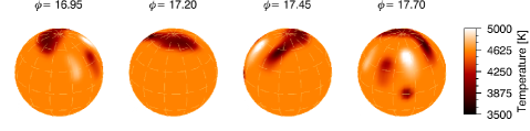
(b)

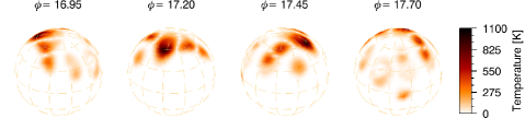
(c)

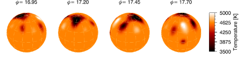
(d)

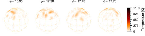
(e)

Figure 4: Test #1 of the influence of phase gaps and filled gaps. Each image is shown in four spherical projections $90^{\circ}$ apart. a) Input map. This map is identical to the first reconstruction from season 2007/08 (DI #8 from 2007.67) with a total of 21 phases. b) The reconstruction when ignoring phases no. 4-9 in the inversion process. c) The (absolute) difference $a-b$. d) The reconstruction when the phase gap is filled with phases from the following stellar rotation. e) The (absolute) difference $a-d$.

(a)

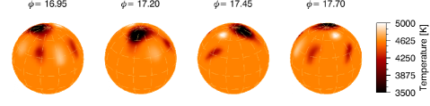
(b)

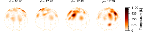
(c)

(d)

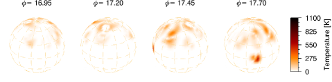
(e)

Figure 5: Test #2 of the influence of phase gaps and filled gaps. Each image is shown in four spherical projections $90^{\circ}$ apart. a) Input map. This map is identical to the first reconstruction from season 2007/08 (DI #8 from 2007.67) with a total of 21 phases. b) The reconstruction when ignoring phases no. 10-15 in the inversion process. c) The (absolute) difference $a-b$. d) The reconstruction when the phase gap is filled with phases from the following stellar rotation. e) The (absolute) difference $a-d$.

4.3 Phase selection and gap filling

To later quantify the continuous evolution of spots based on consecutive Doppler maps, we first deal with the inherent limitations of our phase coverage. In certain circumstances it is difficult to compare consecutive maps that had different phase coverage and that even contained some larger observational gaps (several tenths of a phase) at different rotational phases at different times. The effect of phase gaps on the recovery of individual spots had been simulated by many authors in the past (e.g., Rice & Strassmeier, 2000, and references therein). Generally, Doppler imaging is very robust against small phase gaps but large phase gaps may introduce spurious spots at surface locations not covered by the data.

Fig. 4 and 5 show our simulations with iMap based on real data of XX Tri. During the season 2007/08, STELLA has covered two consecutive stellar rotations completely with one observation per night (DI #8 from 2007.67 and DI #9 from 2007.73, amounting to 21 phases from 23 nights per rotation). From DI #8, we removed six consecutive phases to create an artificial phase gap of $90^{\circ}$ (0$\aas@@fstack{p}$25), and compared the resulting map with the original map (Fig. 4a-c). The two darkest and biggest spots at phases around 17$\aas@@fstack{p}$25 and 17$\aas@@fstack{p}$55 could not be separated anymore. The larger spot loses a big part of its area, which is seen in the difference map in Fig. 4c with a temperature similar to the difference between photospheric and spot temperature. In the next step, we filled these gaps with observations from the following stellar rotation (DI #9) and again compared the resulting map with the original map (Fig. 4d-e). All individual spots are now reconstructed with no changes of their size or temperature exceeding the expected errors driven by the S/N of the data. Fig. 5a-c shows another simulation of the same data with an artificial phase gap of $90^{\circ}$ but at a different rotational phase. Here, the smaller spot at phase around 17$\aas@@fstack{p}$55 has almost completely vanished, whereas it is recovered for the case with gap filling (Fig. 5d-e). We further verified this method on a few other Doppler images with the same result (not shown).

We conclude that large ($\approx$ 90$\degr$) phase gaps have a strong impact on the recovery of the global stellar spot distribution. It affects not only their size and shape but also their location. For smaller spots located within or near the missing phases it affects even their existence. However, when we compare the original map with the maps where the missing phases were filled by phases from one rotation earlier or later, we see a significantly better agreement. This is the case even if the spot distribution had evolved in the meantime. Based on these simulations, we have a simple method to minimize the systematics due to phase gaps. This is only a first-order approximation because the spot evolution within the missing surface area remains unknown. Fig. 23 shows the phase coverage and gap filling of each Doppler image for all seasons, if applicable. Real phase gaps ranged between 1-13 d or 0$\aas@@fstack{p}$04-0$\aas@@fstack{p}$54 at the extremes, but with typical values more near $\approx$ 4 d or 0$\aas@@fstack{p}$17.

For two out of the 36 Doppler images, we had to use phases from two rotations earlier and/or later, as there were no observations closer in time available. In the first case (DI #5) we filled a gap of 5 d (0$\aas@@fstack{p}$21) with two phases. To minimize a possible smearing effect, one phase was taken from two rotations earlier and one from two rotations later. In the case of DI #20, we had to deal with a small number of existing phases in addition. In general, we would not have taken this rotation into account, but in this particular case, we would have only four maps for the observing season 2007/08, two consecutive maps at the beginning and two consecutive maps at the end of the season, which would have severely limited our coverage for this season. We will rediscuss this explicitly in Sect. 5.1 in terms of spot-area evolution.

Table 3 summarizes our Doppler-image log. The year indicates the mid-time of the Doppler image, followed by its Heliocentric Julian Date (HJD) range, the time $\Delta t$ elapsed in days, the number of spectra $N$, the largest phase gap in number of consecutive days (the rotation period is 24 d), and the number of observations from following or preceding stellar rotations that were used to fill phase gaps. In total, we obtained 36 individual Doppler images, each with between 11 to 24 spectra.

4.4 Image analysis: definition of the spot area

One parameter to be extracted from each image is the surface area of a spot. Its measurement depends on the definition where a spot ends and where the undisturbed photosphere begins. Our inversion code is completely free in the reconstruction and usually recovers an irregular spot morphology. Furthermore, the images contain small-scale structures, which seem to appear or disappear from one rotation to another and/or move to different longitudes/latitudes on timescales that are likely shorter than a stellar rotation. These structures often appear as hot spots or as a pair of a hot and a cool spot (but not necessarily along the same isoradial line which would indicate an artifact). The appearance of elongated appendages to the polar spot, or spots that appear connected to another spot, are further complications for determining a spot’s area. Because of inherent limitations of the spatial surface resolution due to the low $v\sin i$, as well as to a lesser extent also due to the choice of regularization during the inversion, these spot configurations cannot easily be separated from each other anymore. Simple area integration of the disk within a certain temperature difference would thus lead to erroneous spot areas.

We define the spot area by fitting artificial spot models to the maps. Our artificial spots have circular shapes of arbitrary size, but a constant temperature of 3500 K. From photometric spot-modeling with spot temperature as free parameter the derived temperature difference $\Delta T$ = $T_{\rm phot}$ $-$ $T_{\rm spot}$ were determined to 1100 K (Strassmeier & Olah, 1992) and 1280 K (Eker, 1995) as well as in the range of 650-1200 K (Hampton et al., 1996) for various epochs. Furthermore, the superspot on the first Doppler image had a temperature difference of 1300 K (Strassmeier, 1999). These values are in agreement with the derived spot temperatures of $\approx$ 3500 K from our Doppler images for long-lived spot structures. As our focus lies in the evolution of starspots, i.e., their decay or growth, we investigate mainly large-scale spot structures that are repeatedly reconstructed from one stellar rotation to the next.

Our method is based on the spot-modeling procedure used in light-curve analysis (e.g., Ribárik et al., 2003), where an appropriate number of spots with circular shape and a defined temperature is taken as input. An initial guess of the spot’s location and radius was taken directly from the observed Doppler images. With these starting values, we calculated the best fit with an area- and temperature-weighted Monte Carlo (MC) method and thus extracted a definition-dependent, best-effort spot location and area. Within the three-parameter space (longitude, latitude, radius) 10,000 random positions were generated, using a range of $15^{\circ}$ for each parameter, and then cross correlated with the original Doppler map. From the best 100 correlation maps (which corresponds to $\sqrt{N}$), the mean values and their standard deviations are determined. In the following, spot area always refers to the spot area deduced from this analysis.

The area of the individual spots from the spot-model fits is summarized in Table 3 in units of solar hemispheres (SH). To estimate the quality of the spot-model fit, we compared the total spotted area between the spot model and the Doppler image. To determine the total spotted area of the Doppler image, a temperature weighting by analogy to the MC method was used. We obtain the total spotted area such that each spotted segment $i$ attributes a certain fraction of its area $a_{i}$ to the total spotted area dependent on its temperature given by

$$A_{\rm total}=\sum_{i}a_{i}\frac{(T_{\rm eff}-T_{i})}{(\Delta T)_{\rm max}}\ ,$$ (2)

where $(\Delta T)_{\rm max}$ = $(T_{\rm phot}$ $-$ $T_{\rm spot})_{\rm max}$ = 1120 K. The small-scale surface structures, cool and hot spots, were not counted into the total spotted area. The quality of the spot-model fits is given in Table 3 in terms of the uncertainty of the spot models, where all our spot models lie within 1 $\sigma$. The absolute scale of the area units in m² is set by the stellar radius of 10.9 R_⊙. Formally, the stellar surface of XX Tri is 724 Gm² and thus 118.8 times the surface of the Sun or 1 SH $\approx$ 0.8 % of an hemisphere of XX Tri.

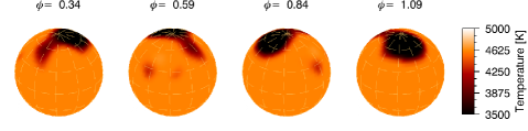
(a)

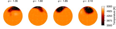
(b)

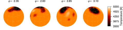
(c)

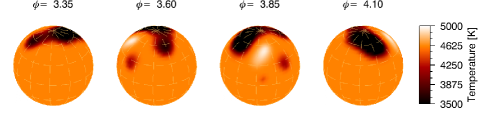
(d)

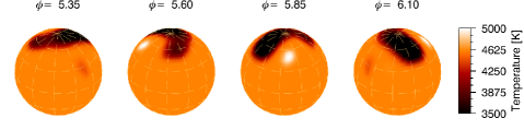
(e)

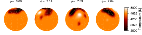
(f)

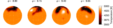
(g)

Figure 6: Doppler images of XX Tri for the observing season 2006/07. Each image is shown in four spherical projections separated by $90^{\circ}$. The rotational shift between consecutive images is corrected, i.e., the stellar orientation remains the same from map to map and from season to season. The time difference between each Doppler image is indicated in units of rotational phase $\phi$.

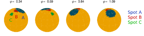
(a)

(b)

(c)

(d)

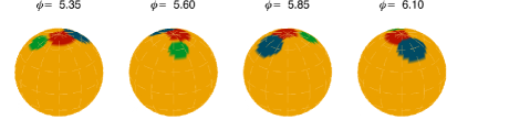
(e)

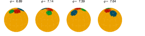
(f)

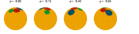
(g)

Figure 7: Spot-model fits of the Doppler images in Fig. 6. Each spot is shown with different color/contrast for better visualization.

4.5 Doppler images and spot models

Fig. 6 is a representative figure for our results and shows all maps for the observing season 2006/07. Seven consecutive Doppler images are reconstructed from a total of $\approx$ 9.5 stellar rotations. All maps show a large polar spot with a temperature of $\approx$ 3500 K. During this season, the polar spot drifted apart and changed its morphology from almost circular to an elongated spot form. This drift could be a sign of differential rotation and is investigated further in Section 5.3. Furthermore, a smaller high-latitude spot with a temperature of around 3800 K is reconstructed. It is seen that the larger spot approached the smaller spot. Because of the inherent technical limitations of Doppler imaging, the surface resolution near the rotational pole is poor and thus spot separations not well constrained. Therefore, one cannot say whether the large spot is a monolithic structure or being a conglomerate of several smaller spots. Besides the polar spot, scattered small cool and/or hot spots are visible at latitudes between 0-60^∘ with absolute temperatures between 4200 to 5000 K.

Table 3: Doppler image log, fit quality, surface temperature, and spot areas. Detailed information is given in Section 4.3-4.5.

DI	Year	HJD range	$\Delta t$	$N$	$\phi$-gap	$N$-fill	RMS	RMS	Temperature (K)		Spot area (SH)
#		(2450000+)	(d)		(d)			($\sigma_{\rm spot}$)	$T_{\rm max}$	$T_{\rm mean}$	Spot A	Spot B	Spot C	Spot D	Spot E	Spot Total
1	2006.58	3935-3963	28	15	4	2	0.0048	0.6	4667	4470	$9.2\pm 0.3$	$1.1\pm 0.6$	$1.3\pm 0.8$	—	—	$11.5\pm 1.0$
2	2006.64	3959-3980	21	19	3	0	0.0046	0.6	4731	4477	$8.5\pm 0.5$	$1.5\pm 0.5$	$1.2\pm 0.7$	—	—	$11.2\pm 0.9$
3	2006.71	3966-4015	49	14	5	3	0.0047	0.7	4796	4489	$8.1\pm 0.6$	$2.1\pm 0.6$	$1.6\pm 0.9$	—	—	$11.8\pm 1.0$
4	2006.78	4007-4050	43	18	7	3	0.0047	0.7	4961	4476	$7.2\pm 0.7$	$2.6\pm 0.5$	$2.4\pm 0.7$	—	—	$12.2\pm 0.8$
5	2006.91	4011-4108	97	17	5	3	0.0047	0.8	5059	4477	$6.0\pm 0.5$	$3.3\pm 0.5$	$3.0\pm 1.1$	—	—	$12.3\pm 1.1$
6	2007.01	4092-4138	46	16	5	2	0.0044	0.5	5052	4492	$5.4\pm 0.6$	$3.7\pm 0.6$	$3.1\pm 1.2$	—	—	$12.2\pm 1.3$
7	2007.14	4124-4161	37	19	5	2	0.0043	0.7	5125	4486	$5.4\pm 0.7$	$3.9\pm 0.6$	$3.2\pm 1.1$	—	—	$12.5\pm 1.3$
8	2007.67	4333-4356	23	21	3	0	0.0040	0.4	5129	4541	$5.5\pm 0.5$	$1.6\pm 0.4$	—	—	—	$7.1\pm 0.8$
9	2007.73	4357-4380	23	21	2	0	0.0035	0.4	5027	4537	$5.2\pm 0.4$	$1.8\pm 0.7$	—	—	—	$7.0\pm 0.9$
10	2007.87	4362-4475	113	15	13	8	0.0033	0.7	4912	4538	$4.1\pm 0.7$	$2.6\pm 0.3$	—	—	—	$6.7\pm 0.7$
11	2008.05	4468-4512	44	19	4	1	0.0037	0.6	4685	4534	$4.3\pm 0.7$	$2.5\pm 0.4$	—	—	—	$6.8\pm 0.7$
12	2008.12	4481-4516	35	15	5	2	0.0038	0.6	5188	4524	$4.1\pm 0.5$	$2.6\pm 0.5$	—	—	—	$6.6\pm 0.4$
13	2008.53	4649-4671	22	20	2	0	0.0040	0.5	4903	4503	$4.8\pm 0.2$	$3.2\pm 0.3$	—	—	—	$8.0\pm 0.4$
14	2008.60	4673-4696	23	22	3	0	0.0037	0.5	4839	4501	$5.5\pm 0.3$	$3.0\pm 0.4$	—	—	—	$8.5\pm 0.5$
15	2008.73	4722-4744	22	14	5	0	0.0038	0.7	4845	4501	$6.4\pm 0.4$	$2.0\pm 0.2$	—	—	—	$8.4\pm 0.4$
16	2008.80	4726-4790	64	15	7	5	0.0034	0.5	4745	4497	$7.5\pm 0.5$	$1.6\pm 0.4$	—	—	—	$9.1\pm 0.6$
17	2008.88	4775-4798	23	16	3	0	0.0035	0.4	5057	4503	$8.0\pm 0.7$	$0.7\pm 0.2$	—	—	—	$8.7\pm 0.8$
18	2008.94	4799-4822	23	15	4	0	0.0032	0.3	5004	4508	$8.1\pm 0.6$	$0.6\pm 0.3$	—	—	—	$8.8\pm 0.7$
19	2009.07	4844-4873	29	16	5	2	0.0035	0.9	5193	4493	$8.2\pm 0.4$	$1.2\pm 0.3$	—	—	—	$9.4\pm 0.5$
20	2009.60	5039-5066	27	18	5	1	0.0033	0.3	4918	4522	$7.8\pm 1.2$	$2.9\pm 0.4$	—	—	—	$10.7\pm 1.3$
21	2009.67	5039-5083	44	17	6	2	0.0035	0.7	4825	4500	$8.1\pm 1.0$	$3.3\pm 0.4$	—	—	—	$11.3\pm 1.1$
22	2009.86	5135-5161	26	17	4	1	0.0039	0.9	5061	4495	$8.3\pm 1.1$	$4.7\pm 0.5$	—	—	—	$13.0\pm 1.1$
23	2009.93	5154-5173	19	16	11	3	0.0036	0.4	5001	4511	$7.4\pm 1.1$	$4.8\pm 0.3$	—	—	—	$12.2\pm 1.1$
24	2010.06	5207-5224	17	17	7	0	0.0035	0.6	5146	4506	$6.8\pm 0.7$	$4.9\pm 0.6$	—	—	—	$11.6\pm 1.0$
25	2010.59	5401-5447	46	12	6	4	0.0029	0.6	4935	4535	$4.5\pm 0.7$	$3.3\pm 0.3$	$0.9\pm 0.6$	—	—	$8.7\pm 0.9$
26	2010.67	5429-5452	23	19	2	0	0.0031	0.4	5088	4538	$4.0\pm 0.7$	$3.1\pm 0.4$	$1.1\pm 0.6$	—	—	$8.1\pm 0.9$
27	2010.74	5439-5496	57	13	7	3	0.0029	0.9	4967	4532	$3.2\pm 0.4$	$2.4\pm 0.6$	$1.5\pm 0.7$	—	—	$7.2\pm 0.9$
28	2010.84	5467-5512	45	17	7	2	0.0030	0.9	4943	4522	$2.6\pm 0.4$	$1.5\pm 0.6$	$2.4\pm 0.6$	—	—	$6.5\pm 0.7$
29	2011.12	5595-5614	19	11	5	0	0.0021	0.5	4620	4513	—	—	—	$5.1\pm 0.5$	$2.3\pm 0.4$	$7.4\pm 0.5$
30	2011.61	5774-5797	23	18	3	0	0.0033	0.3	4758	4493	$4.7\pm 0.6$	$2.9\pm 0.4$	$1.2\pm 0.6$	—	—	$8.8\pm 0.7$
31	2011.68	5799-5822	23	24	1	0	0.0032	0.4	4756	4501	$4.5\pm 0.7$	$2.5\pm 0.8$	$1.7\pm 0.6$	—	—	$8.8\pm 0.8$
32	2011.81	5830-5879	49	17	7	2	0.0029	0.8	4649	4509	$3.7\pm 0.7$	$1.4\pm 0.7$	$3.1\pm 0.4$	—	—	$8.2\pm 1.0$
33	2011.88	5871-5894	23	16	4	0	0.0025	0.9	4722	4501	$3.0\pm 0.5$	$2.7\pm 0.8$	$3.4\pm 0.3$	—	—	$9.1\pm 0.8$
34	2012.01	5919-5940	21	20	3	0	0.0027	0.4	4664	4486	$3.6\pm 0.7$	$3.4\pm 0.9$	$2.6\pm 0.4$	—	—	$9.6\pm 1.0$
35	2012.08	5944-5967	23	18	3	0	0.0026	0.7	4620	4506	$3.3\pm 0.7$	$4.2\pm 0.9$	$1.7\pm 0.4$	—	—	$9.2\pm 1.1$
36	2012.19	5983-6006	23	17	3	0	0.0031	0.3	4767	4477	$3.6\pm 0.7$	$5.8\pm 0.6$	$0.6\pm 0.4$	—	—	$10.0\pm 0.8$

Comparing our new Doppler images with the first image published by Strassmeier (1999) shows a very good agreement of spot locations and spot temperatures, despite $\approx$ 10-year time difference. In both cases, the largest spot appears near the pole with a temperature of around 3500 K. Smaller cool/hot spots appear on lower latitudes, again with comparable temperature differences. The super spot from 1998 with an area of approximately 11 % of the entire stellar surface is much larger than the largest recovered spots that we present. This is expected because the star appeared to be in its brightest stage ever in 2009. In parallel, the rotationally-modulated photometric light curves show a small amplitude compared to that in 1998. During the season 1998/99 a record amplitude of $\approx$ $0\aas@@fstack{m}6$ in $V$ was observed in comparison to an amplitude of $<$ $0\aas@@fstack{m}4$ during the seasons from 2006/07 to 2011/12 (see Oláh et al., 2014).

In Fig. 7 the best spot-model fits for observing season 2006/07 are shown. Three artificial spots were sufficient to reach a high correlation for all Doppler images in this season. Two spots were utilized to represent the large polar spot and to model its drift during almost ten stellar rotations. The third spot represented the smaller high-latitude spot on the opposite hemisphere. All other cool and/or hot spots at lower latitudes with no or only very short continuous appearance were ignored and therefore not implemented in the spot-model analysis.

Doppler images and spot models for the observing seasons 2007-12 are shown in Fig. 11-20. The observed and inverted line profiles of each Doppler image are given in Fig. 21 and 22. Table 3 lists the fit quality between observed ($x_{i,O}$) and calculated ($x_{i,C}$) profiles,

$$RMS=\sqrt{\frac{1}{n}\sum_{i=1}^{n}(x_{i,O}-x_{i,C})^{2}}\ ,$$ (3)

where $n$ is the total number of points of all line profiles used during the inversion. Table 3 also tabulates the maximum and mean surface temperatures of each Doppler image.

5 Results

5.1 Spot area evolution

In each observing season, we see both decay and growth of individual spots. From these spots we infer a linear area decay/formation law of form

$$dA(t)/dt=D\ .$$ (4)

As known from sunspot-decay studies (e.g., Martínez Pillet, 2002), the application of a linear law is the most appropriate way to describe sunspot decay as well as sunspot growth rates. Fig. 8 shows the area evolution of the total spotted area of XX Tri as well as of the individual spots from the spot models for each season. The numerical values of $D$ for each spot together with the overall mean are summarized in Table 4.

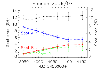
(a)

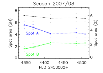
(b)

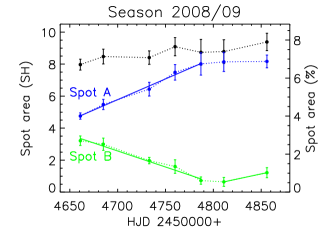
(c)

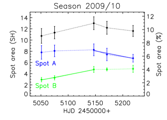
(d)

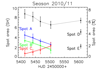
(e)

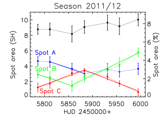
(f)

Figure 8: Spot area evolution on XX Tri from 2006 to 2012. Shown are the seasonal evolution of the individual spots (dotted colored lines) for each observing season. The solid (colored) lines represent linear fits to the decay or growth of a spot. The black dotted line represents the total spotted area. The spot area is given in solar hemispheres on the left axis (1 SH = 3.05 $\mathrm{Gm^{2}}$) and relative to the total area of a stellar hemisphere of XX Tri on the right axis.

Season 2006/07. Three artificial spots are sufficient to match the observed spot distribution in this season. The three spots appear partly merged and make up for the elongated polar-spot appendage in the Doppler images. In the case of overlapping spots, the overlapped area refers to the larger spot. The two overlapping spots, A and B, fragment, while the larger spot A shrinks and the smaller spot B waxes. Between DI #1-6 ($\Delta t$ $\approx$ 6.5 $P_{\rm rot}$) spot A loses around 40 % of its area from 9.2 to 5.4 SH ($D$ = $-$0.025 $\pm$ 0.003 SH/day), while the smaller spot B increases to more than three times its area from 1.1 to 3.7 SH ($D$ = +0.017 $\pm$ 0.004 SH/day). It seems that spot A “feeds” spot B, suggesting flux transport between these two spots. Between DI #6-7 both spots A and B remain almost constant in area. Spot C is located on the opposite hemisphere with a longitudinal shift of around $180^{\circ}$. Between DI #2-5 ($\Delta t$ $\approx$ 5.5 $P_{\rm rot}$) it waxes to almost three times its area from 1.2 to 3.0 SH ($D$ = +0.020 $\pm$ 0.012 SH/day). Afterwards, spot C remains almost constant in area. If we were to exclude DI #5 (see Sect. 4.3), the determined values of $D$ would be $-$0.024 $\pm$ 0.004 SH/day for spot A, +0.017 $\pm$ 0.005 SH/day for spot B, and +0.016 $\pm$ 0.010 SH/day for spot C, respectively.

Season 2007/08. We concentrate on the two larger spots (at phases around 17$\aas@@fstack{p}$25 and 17$\aas@@fstack{p}$55) for a meaningful analysis of spot area evolution. Both spots A and B are separated by around a quarter of rotation in DI #8. During the observing season they merge, as the larger spot A rotates much slower near the pole than the smaller spot B, which is located at mid-latitudes. This indicates that differential rotation is detectable as shown in Sect. 5.3. Between DI #8-10 ($\Delta t$ = 3 $P_{\rm rot}$) spot A loses around 25 % of its area from 5.5 to 4.1 SH ($D$ = $-$0.021 $\pm$ 0.012 SH/day), while spot B increases to almost two times its area from 1.6 to 2.6 SH ($D$ = +0.014 $\pm$ 0.007 SH/day). This phenomenon of two spots interacting with each other, while one spot is decaying and the other is growing, has also been detected in the previous season. If we were to exclude DI #10 (see Sect. 4.3), a reliable determination of $D$ for this season would not have been possible because of the time sampling of the Doppler images. However, removing it from the entire time series has no impact on the mean decay rate.

Season 2008/09. Two spots are sufficient to characterize the spot evolution during this season. The two spots, A and B, are very close and appear connected to each other as seen in DI #13. The large spot A increases from 4.8 to 8.0 SH ($D$ = +0.026 $\pm$ 0.004 SH/day) between DI #13-17 ($\Delta t$ $\approx$ 5 $P_{\rm rot}$) and afterwards remains almost constant in area. Within the same time span, the smaller spot B loses in area from 3.2 to 0.7 SH ($D$ = $-$0.020 $\pm$ 0.003 SH/day). After an almost complete decay, it starts to increase to two times its area from 0.6 to 1.2 SH ($D$ = +0.013 $\pm$ 0.009 SH/day) between DI #18-19 ($\Delta t$ $\approx$ 2 $P_{\rm rot}$). As in the previous season, indications of differential rotation are seen. Spot A is located nearer to the pole than spot B and therefore both spots get separated from each other.

Season 2009/10. Again, two spots are adequate to match the observed spot distribution throughout this season. Both spots A and B are located at opposite hemispheres with a longitudinal shift of around $180^{\circ}$. Between DI #20-22 ($\Delta t$ = 4 $P_{\rm rot}$) the smaller spot B waxes to around 160 % its area from 2.9 to 4.7 SH ($D$ = +0.019 $\pm$ 0.007 SH/day), whereas the larger spot A remains almost constant in area. Between DI #22-24 ($\Delta t$ = 3 $P_{\rm rot}$) the larger spot A loses in area from 8.3 to 6.8 SH ($D$ = $-$0.019 $\pm$ 0.016 SH/day), whereas the smaller spot B remains almost constant in area.

Season 2010/11. During this season three spots are required to characterize the spot evolution. The two large polar spots, A and B, are located at opposite hemispheres with a longitudinal shift of around $150^{\circ}$ and are moving toward each other. Between DI #25-28 ($\Delta t$ $\approx$ 4 $P_{\rm rot}$) both spots A and B lose in area from 4.5 to 2.6 SH ($D$ = $-$0.021 $\pm$ 0.008 SH/day) and 3.3 to 1.5 SH ($D$ = $-$0.020 $\pm$ 0.007 SH/day), respectively. During the same time span, the smaller spot C increases from 0.9 to 2.4 SH ($D$ = +0.017 $\pm$ 0.009 SH/day) and moves toward higher latitudes. There is a large time gap of around four rotations between DI #28-29. During this time span, the spot configuration obviously changes to a two-spot-model. As it is not clear whether one can identify these spots with spots from DI #25-28, we decide to regard them separately. These two polar spots, D and E, are located at opposite hemispheres with a longitudinal shift of around $180^{\circ}$. This spot configuration is almost identical with the first DI (#30) of the following observational season.

Season 2011/12. Again, three spots are sufficient to match the observed large-scale spot distribution during this season. As in the first season, the three spots appear partly merged and make up for the elongated polar-spot appendage in the Doppler images. The two spots, A and B, are located at opposite hemispheres with a longitudinal shift of around $180^{\circ}$. This spot distribution is very similar to that at the end of the previous season. The larger spot A fragments into two smaller spots, A and C, between DI #30-32. Spot C is located very close to the pole and rotates much slower than the other two spots A and B. Between the time of DI #33-36 spot C merges with spot B. Therefore, it again suggests flux transport between spot A and B. Spot A loses in area from 4.5 to 3.0 SH ($D$ = $-$0.021 $\pm$ 0.012 SH/day) between DI #31-33 ($\Delta t$ $\approx$ 3 $P_{\rm rot}$) and remains almost constant in size afterwards. Spot B loses in area from 2.9 to 1.4 SH ($D$ = $-$0.021 $\pm$ 0.011 SH/day) between DI #30-32 ($\Delta t$ = 3 $P_{\rm rot}$) and waxes between DI #32-36 ($\Delta t$ $\approx$ 6 $P_{\rm rot}$) up to 5.8 SH ($D$ = +0.030 $\pm$ 0.006 SH/day). Spot C increases in area up to 3.4 SH ($D$ = +0.023 $\pm$ 0.006 SH/day) between DI #30-33 and decays between DI #33-36 ($\Delta t$ $\approx$ 4.5 $P_{\rm rot}$) almost completely ($D$ = $-$0.024 $\pm$ 0.005 SH/day).

Finally, if we exclude Doppler images #5 and #10, our spot area evolution analysis would lead to an identical mean value for spot decay (¡$D$¿ = $-$0.022 $\pm$ 0.002 SH/day) and only a marginally increased mean value for spot formation (¡$D$¿ = +0.022 $\pm$ 0.002 SH/day). Therefore, we include them in our analysis. Furthermore, we repeated the entire analysis also for the scattered small cool and/or hot spots at low latitudes. Their respective values of $D$ (for small cool spots $\pm$ 0.02 for growth and decay, respectively; hot spots $\pm$ 0.03) scatter within the range of the large-scale spots, but the time sampling is such that we can not determine a true beginning nor ending of the evolution.

Table 4: Individual spot decay and growth rates. Derived values represent a linear area decay law of form $dA(t)/dt$ = $D$. $D$ is given in solar hemispheres (SH) per day (1 SH = 3.05 $\mathrm{Gm^{2}}$).

Season	Spot	DI #	$D$ (SH/day)	type
2006/07	A (blue)	1-6	$-0.025\pm 0.003$	decay
	B (red)	1-6	$+0.017\pm 0.004$	growth
	C (green)	2-5	$+0.020\pm 0.012$	growth
2007/08	A (blue)	8-10	$-0.021\pm 0.012$	decay
	B (green)	8-10	$+0.014\pm 0.007$	growth
2008/09	A (blue)	13-17	$+0.026\pm 0.004$	growth
	B (green)	13-17	$-0.020\pm 0.003$	decay
	B (green)	18-19	$+0.013\pm 0.009$	growth
2009/10	A (blue)	22-24	$-0.019\pm 0.016$	decay
	B (green)	20-22	$+0.019\pm 0.007$	growth
2010/11	A (blue)	25-28	$-0.021\pm 0.008$	decay
	B (green)	25-28	$-0.020\pm 0.007$	decay
	C (red)	25-28	$+0.017\pm 0.009$	growth
2011/12	A (blue)	31-33	$-0.021\pm 0.012$	decay
	B (green)	30-32	$-0.021\pm 0.011$	decay
	B (green)	32-36	$+0.030\pm 0.006$	growth
	C (red)	30-33	$+0.023\pm 0.006$	growth
	C (red)	33-36	$-0.024\pm 0.005$	decay
2006-12			¡$-0.022\pm 0.002$¿	decay
			¡$+0.021\pm 0.002$¿	growth

5.2 Active longitudes

Active longitudes are longitudes on which spots occur preferentially. The analysis of long-term photometric observations as well as time-series Doppler imaging revealed active longitudes on several stars. Berdyugina & Tuominen (1998) found permanent active longitudes on four RS CVn stars. If two active longitudes, which are typically separated by 180^∘, change their spot activity a so-called “flip-flop” occured. This kind of a phenomenon was first noticed on the late-type giant FK Com (Jetsu et al., 1991). The average time between these phenomena is referred to as flip-flop cycle and has been observed to be in the range of a few years up to a decade. An observational overview is given in Berdyugina (2007) and Korhonen & Järvinen (2007). In binary stars, a longitudinal dependence due to tidal effects is suggested (Holzwarth & Schüssler, 2002). Observations show that in binaries preferred longitudes exist on giant components mostly at the substellar points (e.g., Oláh et al., 2002).

(a)

(b)

Figure 9: Active longitudes on XX Tri from 2006 to 2012. a) The overall mean distribution of the spot area (histogram in bins of 15^∘) is shown. The spot area is given in solar hemispheres on the left axis (1 SH = 3.05 $\mathrm{Gm^{2}}$) and relative to the total area of a stellar hemisphere of XX Tri on the right axis. The dashed line represents the phase toward the companion star, whereas the dotted line represents the phase in the opposite direction. b) Spot longitudes as a function of time. Spots A-E from all Doppler images are shown. The filled dots represent the larger spot at any given time. The dashed and dotted lines represent again the phases toward the companion star and in the opposite direction, respectively.

Fig. 26a-f shows the mean longitudinal distributions of all individual spots from our spot-models for each season. There is clear evidence for preferred longitudes during each season but significantly spread out in location because of individual spot evolution. A particularly well-defined pair of active longitudes separated by 180^∘ is seen in season 2009/10. Averaging the longitudinal spot distribution from all 36 Doppler images, we find the most spotted longitude to appear on average in phase toward the unseen companion star ($\pm$ 90^∘; Fig. 9a). Fig. 9b plots the spot centers from our spot-model fits (spots A-E) as a function of time. The larger spot always appears in alternating hemispheres at locations either close to the phase toward the companion star or shifted by around 180^∘. The larger spot appears in between these phases near quadrature possibly only between DI #29-32. Nevertheless, we interpret this behavior as a flip-flop and estimate a tentative period of around two years.

5.3 Differential rotation

Tracking sunspots is a classic technique to measure solar differential rotation and other surface velocity fields like meridional flows (e.g., Wöhl, 2002; Brajša et al., 2002). In case of XX Tri a large number of temperature surface maps with unprecedented good sampling is available, and therefore may enable us to reveal a similarly accurate differential rotation law by tracking individual starspots. Differential rotation has been detected on a number of stars by cross-correlating consecutive Doppler images in longitudinal direction (e.g., Donati & Collier Cameron, 1997; Kővári et al., 2007b). Applying this method to our data, we reconstruct between three and six cross-correlation-function (ccf) maps per observing season, which we average to increase their validity. We did not use the ccf map with DI #29, the last map in season 2010/11, because the time span to the previous map (#28) is comparable large, approximately four rotational periods. Within such a time span, we expect significant local spot evolution. Fig. 24 shows the average ccf maps for each observational season. The resulting grand average ccf map, which consists of 29 ccf maps in total, is given in Fig. 10a.

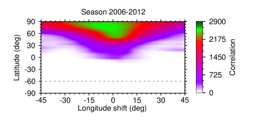
(a)

(b)

Figure 10: a) Grand average cross-correlation-function map from 2006 to 2012. The map represents the average ccf map of all seasonal ccf maps from Fig. 24, thus consisting of 29 ccf maps in total. b) Global differential rotation signature. The dots are the correlation peaks per $5^{\circ}$-latitude bin and their error bars are defined as the FWHM of the corresponding Gaussian fits. The dashed line represents a fit using Eq. 5, whereas the solid line represents a fit using Eq. 6. The parameters for each fit are summarized in Table 5.

We determined the correlation peak for each longitudinal stripe of $5^{\circ}$ width with a Gaussian profile and fitted a standard differential rotation law of the form

$$\Omega(b)=\Omega_{\mathrm{eq}}-\Delta\Omega\sin^{2}(b)\ ,$$ (5)

which is usually used for differential rotation measurements on stars. The parameter $\Omega(b)$ represents the angular velocity at latitude $b$, while $\Delta\Omega$ = $\Omega_{\mathrm{eq}}$ $-$ $\Omega_{\mathrm{pole}}$ represents the difference between the angular velocities at the equator and at the pole, respectively. The surface shear parameter $\alpha$ is defined as $\Delta\Omega/\Omega_{\mathrm{eq}}$, and the lap time as the reciprocal of the rotational shear, i.e., the time it takes for the equator to do a full lap more than the pole.

Alternatively, we fit a differential rotation law of the form

$$\Omega(b)=\Omega_{\mathrm{eq}}+\Omega_{1}\sin^{2}(b)+\Omega_{2}\sin^{4}(b)\ ,$$ (6)

which is usually used for differential rotation measurements on the Sun. In this case the angular velocity at the pole is defined as $\Omega_{\mathrm{pole}}$ = $\Omega_{\mathrm{eq}}$ + $\Omega_{1}$ + $\Omega_{2}$. Fig. 25 and Fig. 10b show the observed differential rotation pattern determined from the ccf maps together with the best fit of the differential rotation following Eq. 5 and Eq. 6. In Table 5 all seasonal fits for differential rotation are listed.

Table 5: Results for differential rotation. Parameters for best fits using Eq. 5 (middle part) and Eq. 6 (right part). The parameter $\Omega_{\mathrm{eq}}$ is fixed for $P_{\mathrm{rot}}$ = 24.0 d in both cases.

Season	$\#$ ccf maps	$\Delta\Omega$ (∘/d)	$\alpha$	lap time (d)	$\Omega_{1}$ (∘/d)	$\Omega_{2}$ (∘/d)	$\alpha$	lap time (d)
2006/07	6	0.05$\pm$0.03	0.003$\pm$0.002	$\approx$6870	0.53$\pm$0.04	–0.68$\pm$0.04	0.010$\pm$0.001	$\approx$2430
2007/08	4	0.30$\pm$0.08	0.020$\pm$0.005	$\approx$1190	0.83$\pm$0.20	–1.35$\pm$0.23	0.035$\pm$0.010	$\approx$690
2008/09	6	0.29$\pm$0.06	0.019$\pm$0.004	$\approx$1240	0.51$\pm$0.16	–0.95$\pm$0.18	0.030$\pm$0.011	$\approx$810
2009/10	4	0.11$\pm$0.04	0.007$\pm$0.003	$\approx$3290	0.22$\pm$0.21	–0.39$\pm$0.24	0.011$\pm$0.012	$\approx$2130
2010/11	3	0.19$\pm$0.06	0.013$\pm$0.004	$\approx$1870	–0.20$\pm$0.25	0.01$\pm$0.33	0.013$\pm$0.058	$\approx$1890
2011/12	6	0.00$\pm$0.04	0.000$\pm$0.003	—	0.64$\pm$0.14	–0.74$\pm$0.17	0.007$\pm$0.002	$\approx$3460
2006-12	29	0.13$\pm$0.04	0.009$\pm$0.003	$\approx$2740	0.45$\pm$0.07	–0.69$\pm$0.09	0.016$\pm$0.003	$\approx$1530

Because most spots on XX Tri appear at high latitudes, Eq. 6 with its $\sin^{4}b$ term leads to a much better fit to the observed shear than Eq. 5. Therefore, we favor Eq. 6 over Eq. 5. All observing seasons show a solar-like differential rotation law with an overall shear parameter of $\alpha$ = 0.016 $\pm$ 0.003 and a lap time of $\approx$ 1500 days. The surface shear on XX Tri is therefore only around a tenth of the solar value.

5.4 Stellar cycle prediction

Because turbulent diffusion is believed to be the dominating effect of spot decay, the decay rate of spot area is directly proportional to the turbulent diffusivity (Meyer et al., 1974; Krause & Rüdiger, 1975),

$$dA/dt=-4\pi\eta_{T}\ .$$ (7)

Using the mean decay rate of $D$ = $-$0.022 $\pm$ 0.002 SH/day from our analysis in Table 4 leads to a turbulent diffusivity of $\eta_{T}$ = (6.3 $\pm$ 0.5) $\times$ 10¹⁴ cm²/s. This value is at minimum one order of magnitude higher than that predicted for solar values, which vary from $10^{10}$ cm²/s (Dikpati & Charbonneau, 1999) to $10^{13}$ cm²/s (Rüdiger & Kitchatinov, 2000). The diffusion timescale for the magnetic field inside the convection zone (CZ) is given by

$$\tau=\frac{L_{CZ}^{2}}{\eta_{T}}\ ,$$ (8)

where $L_{CZ}^{2}$ is the width of the stellar convection zone. Using stellar models calculated with the Yale Rotational stellar Evolution Code (YREC; see Spada et al. (2013) for more details) we estimate a depth of 0.94 $R_{\star}$ for the convection zone of XX Tri. Thus, leading to a magnetic cycle of approximately 26 $\pm$ 6 years.

5.5 A starspot movie

We merged all 36 Doppler images into an animated gif file (xxtri-di-anim.gif), which is available through the A&A video depository or our group web page. It particularly emphasizes surface detail not covered in the spot-decay analysis and shows the general migration and decay trends. It may be used for general demonstration purposes.

The movie shows the same four equidistant surface views as, e.g., in Fig. 6 but just as a function of time. Between each Doppler image a time delay of 250 ms is included.

6 Discussion and summary

Thanks to our robotic STELLA telescopes the present time series of Doppler images resolves 36 single stellar rotations over a time span of six years. The sample is long enough that it enables, for the first time, a direct determination of a starspot decay law. Our target is the K0 giant XX Tri with a rotation period ($\approx$ 24 d) comparable to that of the Sun but being more massive by 26 % and significantly older with an age of $\approx$ 8 Gyrs. This combination of parameters is only possible because the star is a component of a close binary. A comparison with solar analogies is therefore only for general guidance.

The time series enabled the cartography of a variety of surface activity phenomena, such as active longitudes, flip-flops, and differential rotation on XX Tri. However, our main result is a spot decay law leading to a prediction of a magnetic activity cycle solely based on an observationally constrained value of the turbulent magnetic diffusivity. The individual spot decay rates, $dA/dt$ = $D$, scattered between $-0.019$ and $-0.025$ SH/day over the six year observing period with a mean value of $D$ = $-$0.022 $\pm$ 0.002 SH/day. The rates for spot growth were between $+0.013$ and $+0.030$ SH/day with a mean of $D$ = +0.021 $\pm$ 0.002 SH/day and thus of nearly the same amount as the decay. In above units, the spot decay on XX Tri would be of the order of $10^{4}$ times faster than what Bumba (1963) suggested for sunspots. Bumba proposed a mean value for $D$ of $-4.2$ MSH/day. However, the areal size of starspots on XX Tri is also $10^{3}$ to $10^{4}$ times larger than the largest observed sunspots ($\approx$ 10^-3 SH; Baumann & Solanki 2005). From this, we depict a turbulent diffusivity for XX Tri of $\approx$ 6 $\times$ 10¹⁴ cm²/s, a value between 10 to 10,000 times larger than current model values for the solar convection zone (from the surface layers to the bottom of the convection zone). Because the (squared) absolute depth of the convection zone of XX Tri is about 1,200 times larger than that of the Sun (200 Mm), the diffusion timescale becomes comparable to that of the Sun. We obtain an average diffusion time of $\approx$ 26 yr for XX Tri compared to $\approx$ 12 yr for the Sun (the latter for an assumed diffusivity of 10¹² cm²/s).

So far, stellar activity cycles were inferred from long-term chromospheric Ca ii H&K or photospheric $V$-band variations (e.g., Baliunas et al., 1995; Oláh et al., 2007) or from repeated detections of a “flip-flop” phenomenon (see Hackman et al., 2013; Korhonen & Järvinen, 2007). Derived timescales for RS CVn stars range between 2-50 yr. Just recently, Oláh et al. (2014) investigated 28 years of photometry of XX Tri along with two other over-active K giants and found a long-term sinusoidal brightness trend with a length comparable to the length of the data set, i.e., $\approx$ 28 yr. Our diffusivity-based cycle prediction of $\approx$ 26 yr matches this observation surprisingly well despite the comparable shortness of the photometric coverage. XX Tri reached its maximum brightness in 2009 and is in a declining state since then. Removing this overall trend, Oláh et al. (2014) found a second shorter-period variation of approximately 6 yr or an integer multiple of it. No clear explanation for this period, if real, could be given.

As already mentioned in Sect. 4.5, the reconstructed giant spots may be monolithic, but could also be a conglomerate of smaller, unresolved spots. This “classical” uncertainty could in principle impact on the interpretation of the observed decay rate, and thus the cycle length. Assuming that each unresolved spot only decays (and never grows), and does not interact with an other spot fragment, then we should observe on average the same decay rate as if the spot were monolithic. If decay and growth of individual fragments coexist, then our determined decay rate would be just a lower boundary. It then enables a maximum decay rate of  $\approx$ $-0.03$ SH/day, resulting in a cycle length of $\approx$ 19 yr. This cycle period would be close to our determined 1-$\sigma$ uncertainty. On the contrary, no such cycle period was detected from broadband photometry. In addition, a possible cycle length of six years (from photometry) or two years (from flip-flop) would suggest a decay rate of $-0.10$ and $-0.29$ SH/day, respectively; neither of which is supported by our analysis. We conclude that our predicted cycle of $\approx$ 26 yr, including an uncertainty of 6 yr, appears to be the most credible.

Active longitudes are a common feature in rapidly-rotating active stars and there is even some evidence for long-term active longitudes and a 7-yr flip-flop period on the Sun (Berdyugina & Usoskin, 2003). Our Doppler imagery provides evidence for a $\approx$ 2-yr flip-flop period on XX Tri with a preferred longitude typically facing the (unseen) companion star. This is significantly shorter than the 6-yr period from photometric data, but could be the true flip-flop cycle length and thus would identify the 6-yr period just as an alias. From a theoretical perspective, flip-flops possibly represent the nonaxisymmetric component of a mixed-mode dynamo for weakly differentially rotating stars (Elstner & Korhonen, 2005; Moss, 2004). These authors explained flip-flops as an excited nonaxisymmetric dynamo mode, giving rise to two permanent active longitudes in opposite stellar hemispheres, but still need an oscillating axisymmetric magnetic field in parallel. The stability of this kind of a mixed mode is still a matter of discussion.

For XX Tri, our Doppler images indicate a weak solar-like differential rotation of $\alpha$ = 0.016 $\pm$ 0.003, which seems to be a typical value for this kind of rapidly rotating stars. Despite the fact that large-scale mean-field dynamo models predict only a poor tracing quality for its large spots (Korhonen & Elstner 2011; but see also Czesla et al. 2013), numerous differential-rotation laws were deduced from cross correlations of cool features from consecutive Doppler images (at this point we refer to the many references cited in Korhonen & Elstner 2011). Recently, weak solar-like differential rotation was confirmed, e.g., on the K giants IL Hya (Kővári et al., 2014; Weber & Strassmeier, 1998) or $\zeta$ And (Kővári et al., 2012, 2007a), while weak antisolar differential rotation was confirmed on the K-giant $\sigma$ Gem (Kővári et al., 2015, 2007b). Furthermore, weak antisolar differential rotation was claimed for the K giants UZ Lib (Oláh et al., 2003), HD 31993 (Strassmeier et al., 2003), and possibly HU Vir (Strassmeier, 1994). All the latter still in need of further independent verification. For a previous summary on this topic we refer to Weber et al. (2005). XX Tri fits into the differentially rotating giants with approximately ten times weaker surface latitudinal shear when compared to the Sun.

Appendix A Doppler images for the seasons 2007/08 to 2011/12

A.1 Season 2007/08

In Fig. 11 five almost consecutive Doppler images are shown, which cover around eight rotations. In Fig. 12 the spot-model fits of the Doppler images are shown.

(a)

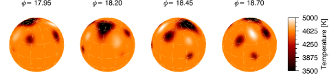
(b)

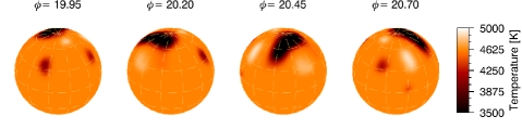
(c)

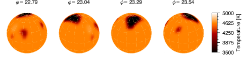
(d)

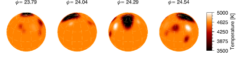
(e)

Figure 11: Doppler images of XX Tri for the observing season 2007/08. Each DI is shown in four spherical projections separated by $90^{\circ}$. The rotational shift between consecutive images is corrected, i.e., the stellar orientation remains the same from map to map and from season to season. The time difference between each Doppler image is indicated in units of rotational phase $\phi$.

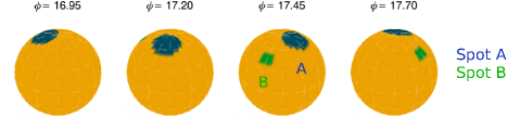
(a)

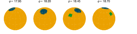
(b)

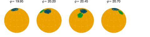
(c)

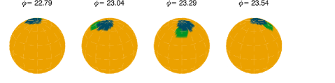
(d)

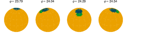
(e)

Figure 12: Spot-model fits of the Doppler images in Fig. 11. Each spot is shown with different color/contrast for better visualization.

A.2 Season 2008/09

In Fig. 13 seven almost consecutive Doppler images are shown, which cover around nine rotations. In Fig. 14 the spot-model fits of the Doppler images are shown.

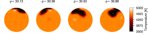
(a)

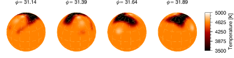
(b)

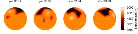
(c)

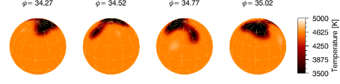
(d)

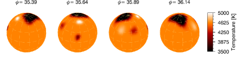
(e)

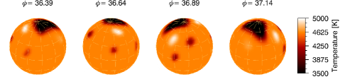
(f)

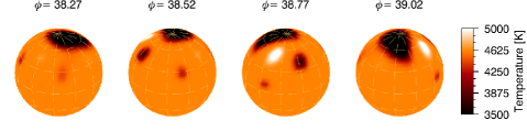
(g)

Figure 13: Doppler images of XX Tri for the observing season 2008/09. Otherwise as in Fig. 11.

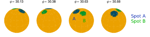
(a)

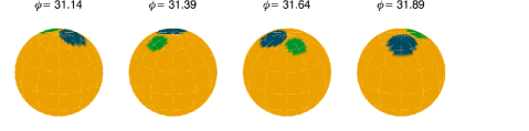
(b)

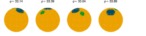
(c)

(d)

(e)

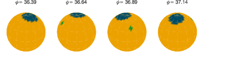
(f)

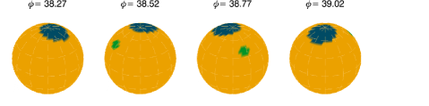
(g)

Figure 14: Spot-model fits of the Doppler images in Fig. 13. Otherwise as in Fig. 12.

A.3 Season 2009/10

In Fig. 15 five almost consecutive Doppler images are shown, which cover around eight rotations. In Fig. 16 the spot-model fits of the Doppler images are shown.

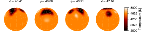
(a)

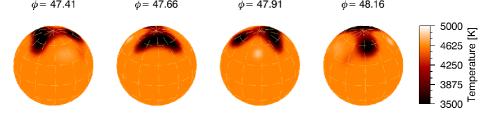
(b)

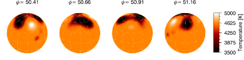
(c)

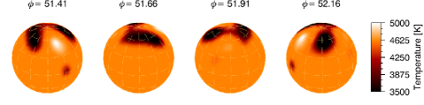
(d)

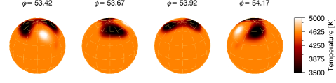
(e)

Figure 15: Doppler images of XX Tri for the observing season 2009/10. Otherwise as in Fig. 11.

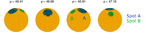
(a)

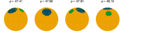
(b)

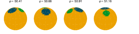
(c)

(d)

(e)

Figure 16: Spot-model fits of the Doppler images in Fig. 15. Otherwise as in Fig. 12.

A.4 Season 2010/11

In Fig. 17 five almost consecutive Doppler images are shown, which cover around nine rotations. In Fig. 18 the spot-model fits of the Doppler images are shown.

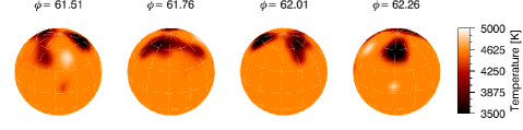
(a)

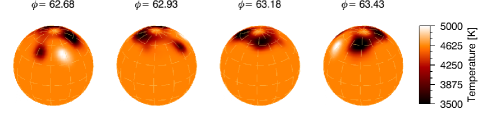
(b)

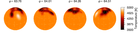
(c)

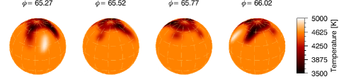
(d)

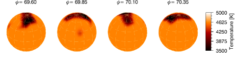
(e)

Figure 17: Doppler images of XX Tri for the observing season 2010/11. Otherwise as in Fig. 11.

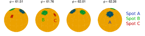
(a)

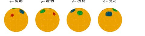
(b)

(c)

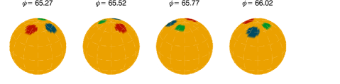
(d)

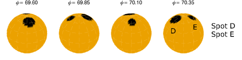
(e)

Figure 18: Spot-model fits of the Doppler images in Fig. 17. Otherwise as in Fig. 12.

A.5 Season 2011/12

In Fig. 19 seven almost consecutive Doppler images are shown, which cover around ten rotations. In Fig. 20 the spot-model fits of the Doppler images are shown.

(a)

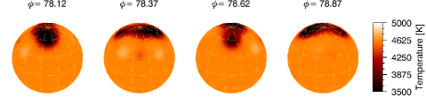
(b)

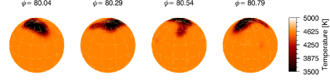
(c)

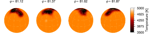
(d)

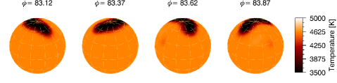
(e)

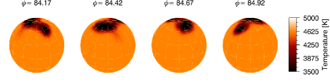
(f)

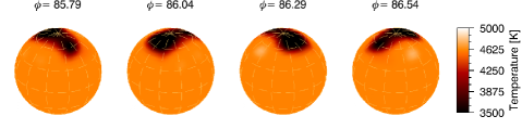
(g)

Figure 19: Doppler images of XX Tri for the observing season 2011/12. Otherwise as in Fig. 11.

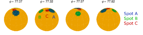
(a)

(b)

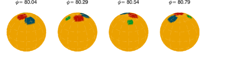
(c)

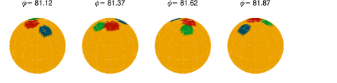
(d)

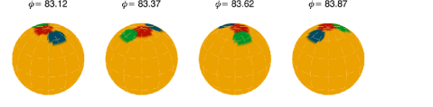
(e)

(f)

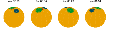
(g)

Figure 20: Spot-model fits of the Doppler images in Fig. 19. Otherwise as in Fig. 12.

Appendix B Line profiles of Doppler images for the seasons 2006/07 to 2011/12

Fig. 21 and Fig. 22 show the observed and inverted line profiles of each Doppler image for all observational seasons.

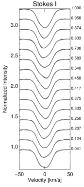
(a) 2006.58

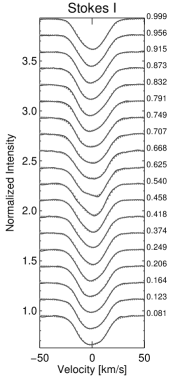
(b) 2006.64

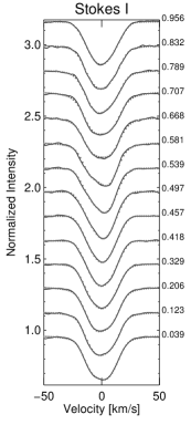
(c) 2006.71

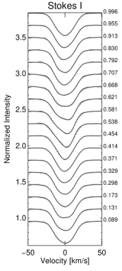
(d) 2006.78

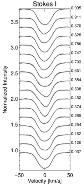
(e) 2006.91

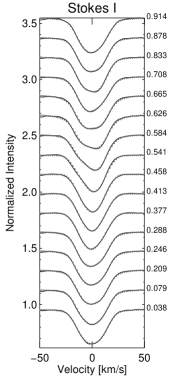
(f) 2007.01

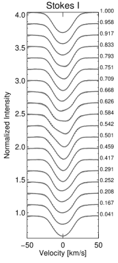
(g) 2007.14

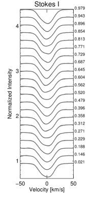
(h) 2007.67

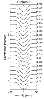
(i) 2007.73

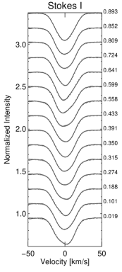
(j) 2007.87

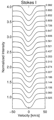
(k) 2008.05

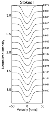
(l) 2008.12

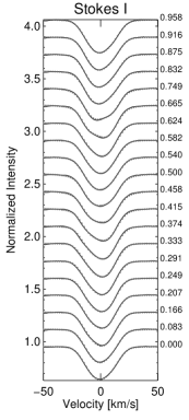
(m) 2008.53

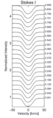
(n) 2008.60

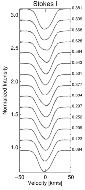
(o) 2008.73

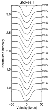
(p) 2008.80

(q) 2008.88

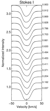
(r) 2008.94

Figure 21: Line profiles of Doppler images #1-18. Each figure shows the observed (solid lines) and inverted (dotted lines) line profiles for one Doppler image stating their mid times and the respective phases. Rotation advances from bottom to the top. Their corresponding RMS-errors are given in Table 3.

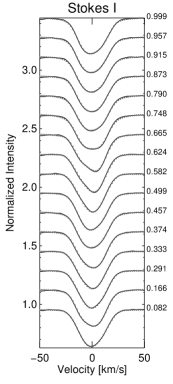
(a) 2009.07

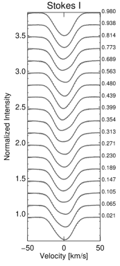
(b) 2009.60

(c) 2009.67

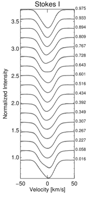
(d) 2009.86

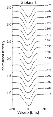
(e) 2009.93

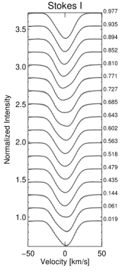
(f) 2010.06

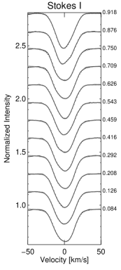
(g) 2010.59

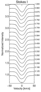
(h) 2010.67

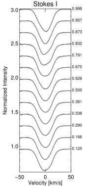
(i) 2010.74

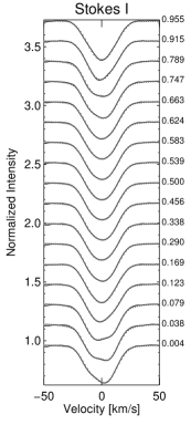
(j) 2010.84

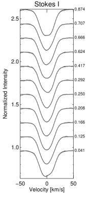
(k) 2011.12

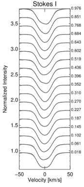
(l) 2011.61

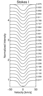
(m) 2011.68

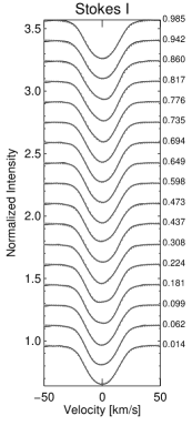
(n) 2011.81

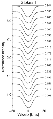
(o) 2011.88

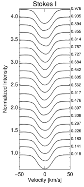
(p) 2012.01

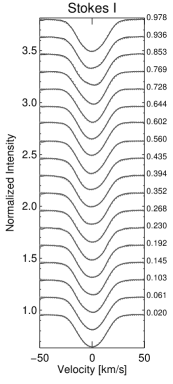
(q) 2012.08

(r) 2012.19

Figure 22: Line profiles of Doppler images #19-36. Otherwise as in Fig. 21.

Appendix C Phase coverage of Doppler images for the seasons 2006/07 to 2011/12

Fig. 23 shows the phase coverage of each Doppler image for all observational seasons.

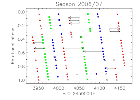
(a)

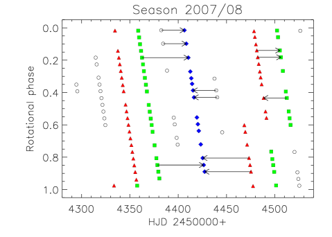
(b)

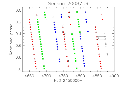
(c)

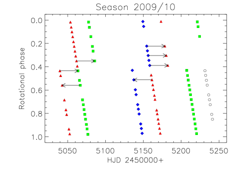
(d)

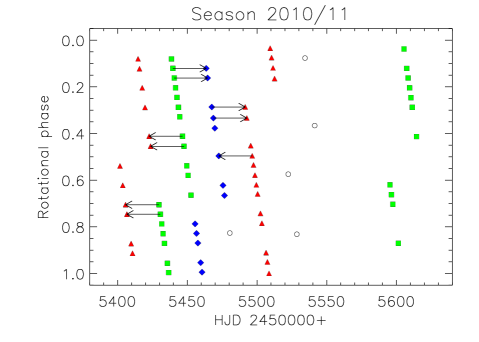
(e)

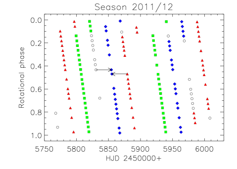
(f)

Figure 23: Phase coverage of Doppler images from 2006 to 2012. Different filled (colored) symbols represents the phases of each individual Doppler image, whereas not-filled circles represents non-used spectra (except for gap filling). The arrows indicate the spectra, which were used to fill up large observational gaps. Detailed information is given in Table 3.

Appendix D CCF-maps and DR-fits for the seasons 2006/07 to 2011/12

Fig. 24 shows the ccf maps from each observing season. In Fig. 25 the observed differential rotation pattern determined from the ccf maps, together with the best fit of the differential rotation following Eq. 5 and Eq. 6 are shown.

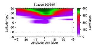
(a)

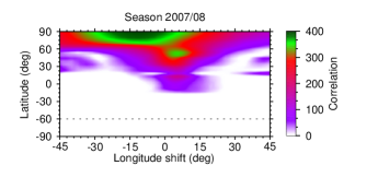
(b)

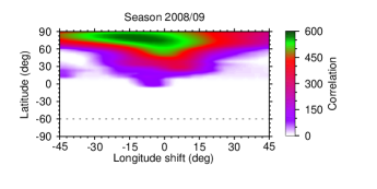
(c)

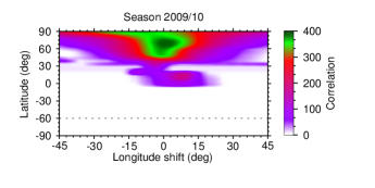
(d)

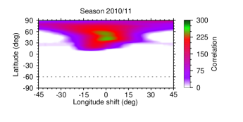
(e)

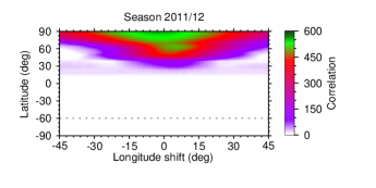
(f)

Figure 24: Cross-correlation function maps from 2006 to 2012. Each map represents the average ccf map for one observing season.

(a)

(b)

(c)

(d)

(e)

(f)

Figure 25: Differential rotation signatures from 2006 to 2012. Analyzing the ccf maps in Fig. 24 reveals a weak solar-like differential rotation. The dots are the correlation peaks per $5^{\circ}$-latitude bin and their error bars are defined as the FWHMs of the corresponding Gaussians. The dashed line represents a fit using Eq. 5, whereas the solid line represents a fit using Eq. 6. The parameters for each fit are summarized in Table 5.

Appendix E Longitudinal spot distribution for the seasons 2006/07 to 2011/12

Fig. 26 shows the mean distribution of the spot area from our spot-model fits for each observing season.

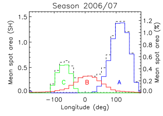
(a)

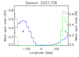
(b)

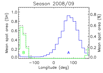
(c)

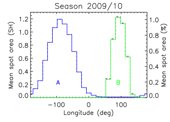
(d)

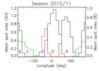
(e)

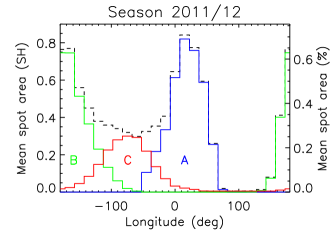
(f)

Figure 26: Longitudinal spot area distribution on XX Tri from 2006 to 2012. Shown are the seasonal mean distributions of the individual spots (solid colored lines) from our spot-model fits for each observing season. The black dashed line represents the total spotted area. The spot area is given in solar hemispheres on the left axis (1 SH = 3.05 $\mathrm{Gm^{2}}$) and relative to the total area of a stellar hemisphere of XX Tri on the right axis.

References

- Allende Prieto (2004) Allende Prieto, C. 2004, Astronomische Nachrichten, 325, 604
- Babcock (1961) Babcock, H. W. 1961, ApJ, 133, 572
- Baliunas et al. (1995) Baliunas, S. L., Donahue, R. A., Soon, W. H., et al. 1995, ApJ, 438, 269
- Barnes et al. (2005) Barnes, J. R., Collier Cameron, A., Donati, J.-F., et al. 2005, MNRAS, 357, L1
- Baumann & Solanki (2005) Baumann, I. & Solanki, S. K. 2005, A&A, 443, 1061
- Berdyugina (2007) Berdyugina, S. V. 2007, Highlights of Astronomy, 14, 275
- Berdyugina et al. (1998) Berdyugina, S. V., Berdyugin, A. V., Ilyin, I., & Tuominen, I. 1998, A&A, 340, 437
- Berdyugina et al. (1999) Berdyugina, S. V., Berdyugin, A. V., Ilyin, I., & Tuominen, I. 1999, A&A, 350, 626
- Berdyugina et al. (2000) Berdyugina, S. V., Berdyugin, A. V., Ilyin, I., & Tuominen, I. 2000, A&A, 360, 272
- Berdyugina & Tuominen (1998) Berdyugina, S. V. & Tuominen, I. 1998, A&A, 336, L25
- Berdyugina & Usoskin (2003) Berdyugina, S. V. & Usoskin, I. G. 2003, A&A, 405, 1121
- Bertelli et al. (2008) Bertelli, G., Girardi, L., Marigo, P., & Nasi, E. 2008, A&A, 484, 815
- Bidelman (1985) Bidelman, W. P. 1985, International Amateur-Professional Photoelectric Photometry Communications, 21, 53
- Bopp et al. (1993) Bopp, B. W., Fekel, F. C., Aufdenberg, J. P., Dempsey, R., & Dadonas, V. 1993, AJ, 106, 2502
- Brajša et al. (2002) Brajša, R., Wöhl, H., Vršnak, B., et al. 2002, Sol. Phys., 206, 229
- Bumba (1963) Bumba, V. 1963, Bulletin of the Astronomical Institutes of Czechoslovakia, 14, 91
- Carroll et al. (2007) Carroll, T. A., Kopf, M., Ilyin, I., & Strassmeier, K. G. 2007, Astronomische Nachrichten, 328, 1043
- Carroll et al. (2008) Carroll, T. A., Kopf, M., & Strassmeier, K. G. 2008, A&A, 488, 781
- Carroll et al. (2009) Carroll, T. A., Kopf, M., Strassmeier, K. G., Ilyin, I., & Tuominen, I. 2009, in IAU Symposium, ed. K. G. Strassmeier, A. G. Kosovichev, & J. E. Beckman, Vol. 259, 437
- Carroll et al. (2012) Carroll, T. A., Strassmeier, K. G., Rice, J. B., & Künstler, A. 2012, A&A, 548, A95
- Castelli & Kurucz (2004) Castelli, F. & Kurucz, R. L. 2004, ArXiv:astro-ph/0405087
- Czesla et al. (2013) Czesla, S., Arlt, R., Bonanno, A., Strassmeier, K. G., & Huber, K. F. 2013, Astronomische Nachrichten, 334, 89
- Dikpati & Charbonneau (1999) Dikpati, M. & Charbonneau, P. 1999, ApJ, 518, 508
- Donati & Collier Cameron (1997) Donati, J.-F. & Collier Cameron, A. 1997, MNRAS, 291, 1
- Eker (1995) Eker, Z. 1995, ApJ, 445, 526
- Elstner & Korhonen (2005) Elstner, D. & Korhonen, H. 2005, Astronomische Nachrichten, 326, 278
- Flower (1996) Flower, P. J. 1996, ApJ, 469, 355
- Gokhale & Zwaan (1972) Gokhale, M. H. & Zwaan, C. 1972, Sol. Phys., 26, 52
- Granzer et al. (2010) Granzer, T., Weber, M., & Strassmeier, K. G. 2010, Advances in Astronomy, 2010
- Gustafsson et al. (2008) Gustafsson, B., Edvardsson, B., Eriksson, K., et al. 2008, A&A, 486, 951
- Hackman et al. (2012) Hackman, T., Mantere, M. J., Lindborg, M., et al. 2012, A&A, 538, A126
- Hackman et al. (2013) Hackman, T., Pelt, J., Mantere, M. J., et al. 2013, A&A, 553, A40
- Hall (1972) Hall, D. S. 1972, PASP, 84, 323
- Hampton et al. (1996) Hampton, M., Henry, G. W., Eaton, J. A., Nolthenius, R. A., & Hall, D. S. 1996, PASP, 108, 68
- Holzwarth & Schüssler (2002) Holzwarth, V. & Schüssler, M. 2002, Astronomische Nachrichten, 323, 399
- Hooten & Hall (1990) Hooten, J. T. & Hall, D. S. 1990, ApJS, 74, 225
- Jabbari et al. (2014) Jabbari, S., Brandenburg, A., Kleeorin, N., Mitra, D., & Rogachevskii, I. 2014, ArXiv e-prints: 1411.4912
- Jetsu et al. (1991) Jetsu, L., Pelt, J., Tuominen, I., & Nations, H. 1991, in Lecture Notes in Physics, Berlin Springer Verlag, Vol. 380, IAU Colloq. 130: The Sun and Cool Stars. Activity, Magnetism, Dynamos, ed. I. Tuominen, D. Moss, & G. Rüdiger, 381
- Jovanovic et al. (2013) Jovanovic, M., Weber, M., & Allende Prieto, C. 2013, Publications de l’Observatoire Astronomique de Beograd, 92, 169
- Käpylä et al. (2012) Käpylä, P. J., Mantere, M. J., & Brandenburg, A. 2012, ApJ, 755, L22
- Käpylä et al. (2011) Käpylä, P. J., Mantere, M. J., & Hackman, T. 2011, ApJ, 742, 34
- Kővári et al. (2007a) Kővári, Z., Bartus, J., Strassmeier, K. G., et al. 2007a, A&A, 463, 1071
- Kővári et al. (2007b) Kővári, Z., Bartus, J., Strassmeier, K. G., et al. 2007b, A&A, 474, 165
- Kővári et al. (2012) Kővári, Z., Korhonen, H., Kriskovics, L., et al. 2012, A&A, 539, A50
- Kővári et al. (2015) Kővári, Z., Kriskovics, L., Künstler, A., et al. 2015, A&A, 573, A98
- Kővári et al. (2014) Kővári, Z., Kriskovics, L., Oláh, K., et al. 2014, in IAU Symposium, ed. P. Petit, M. Jardine, & H. C. Spruit, Vol. 302, 379
- Kloppenborg et al. (2010) Kloppenborg, B., Stencel, R., Monnier, J. D., et al. 2010, Nature, 464, 870
- Korhonen et al. (2007) Korhonen, H., Berdyugina, S. V., Hackman, T., et al. 2007, A&A, 476, 881
- Korhonen & Elstner (2011) Korhonen, H. & Elstner, D. 2011, A&A, 532, A106
- Korhonen & Järvinen (2007) Korhonen, H. & Järvinen, S. P. 2007, in IAU Symposium, ed. W. I. Hartkopf, P. Harmanec, & E. F. Guinan, Vol. 240, 453
- Krause & Rüdiger (1975) Krause, F. & Rüdiger, G. 1975, Sol. Phys., 42, 107
- Künstler (2008) Künstler, A. 2008, Diploma thesis, Landessternwarte Heidelberg
- Kupka et al. (1999) Kupka, F., Piskunov, N., Ryabchikova, T. A., Stempels, H. C., & Weiss, W. W. 1999, A&AS, 138, 119
- Leighton (1964) Leighton, R. B. 1964, ApJ, 140, 1547
- Lindborg et al. (2011) Lindborg, M., Korpi, M. J., Hackman, T., et al. 2011, A&A, 526, A44
- Marsden et al. (2007) Marsden, S. C., Berdyugina, S. V., Donati, J.-F., Eaton, J. A., & Williamson, M. H. 2007, Astronomische Nachrichten, 328, 1047
- Martínez Pillet (2002) Martínez Pillet, V. 2002, Astronomische Nachrichten, 323, 342
- Martinez Pillet et al. (1993) Martinez Pillet, V., Moreno-Insertis, F., & Vazquez, M. 1993, A&A, 274, 521
- Meyer et al. (1974) Meyer, F., Schmidt, H. U., Wilson, P. R., & Weiss, N. O. 1974, MNRAS, 169, 35
- Moradi et al. (2010) Moradi, H., Baldner, C., Birch, A. C., et al. 2010, Sol. Phys., 267, 1
- Moreno-Insertis & Vazquez (1988) Moreno-Insertis, F. & Vazquez, M. 1988, A&A, 205, 289
- Moss (2004) Moss, D. 2004, MNRAS, 352, L17
- Nolthenius (1991) Nolthenius, R. 1991, Information Bulletin on Variable Stars, 3589, 1
- Oláh et al. (2003) Oláh, K., Jurcsik, J., & Strassmeier, K. G. 2003, A&A, 410, 685
- Oláh et al. (2014) Oláh, K., Moór, A., Kővári, Z., et al. 2014, A&A, 572, A94
- Oláh et al. (2007) Oláh, K., Strassmeier, K. G., Granzer, T., Soon, W., & Baliunas, S. L. 2007, Astronomische Nachrichten, 328, 1072
- Oláh et al. (2002) Oláh, K., Strassmeier, K. G., & Weber, M. 2002, A&A, 389, 202
- Petrovay & van Driel-Gesztelyi (1997) Petrovay, K. & van Driel-Gesztelyi, L. 1997, Sol. Phys., 176, 249
- Prugniel & Soubiran (2001) Prugniel, P. & Soubiran, C. 2001, A&A, 369, 1048
- Reiners (2006) Reiners, A. 2006, A&A, 446, 267
- Ribárik et al. (2003) Ribárik, G., Oláh, K., & Strassmeier, K. G. 2003, Astronomische Nachrichten, 324, 202
- Rice (2002) Rice, J. B. 2002, Astronomische Nachrichten, 323, 220
- Rice & Strassmeier (2000) Rice, J. B. & Strassmeier, K. G. 2000, A&AS, 147, 151
- Rüdiger & Kitchatinov (2000) Rüdiger, G. & Kitchatinov, L. L. 2000, Astronomische Nachrichten, 321, 75
- Scharlemann (1981) Scharlemann, E. T. 1981, ApJ, 246, 292
- Scharlemann (1982) Scharlemann, E. T. 1982, ApJ, 253, 298
- Schrijver & Zwaan (1991) Schrijver, C. J. & Zwaan, C. 1991, A&A, 251, 183
- Solanki (2003) Solanki, S. K. 2003, A&A Rev., 11, 153
- Spada et al. (2013) Spada, F., Demarque, P., Kim, Y.-C., & Sills, A. 2013, ApJ, 776, 87
- Starck et al. (1998) Starck, J.-L., Murtagh, F. D., & Bijaoui, A. 1998, Image Processing and Data Analysis (Cambridge University Press)
- Starck et al. (1997) Starck, J.-L., Siebenmorgen, R., & Gredel, R. 1997, ApJ, 482, 1011
- Stix (1989) Stix, M. 1989, The Sun. An Introduction (Springer-Verlag)
- Strassmeier (1994) Strassmeier, K. G. 1994, A&A, 281, 395
- Strassmeier (1999) Strassmeier, K. G. 1999, A&A, 347, 225
- Strassmeier (2009) Strassmeier, K. G. 2009, A&A Rev., 17, 251
- Strassmeier & Bartus (2000) Strassmeier, K. G. & Bartus, J. 2000, A&A, 354, 537
- Strassmeier et al. (1997) Strassmeier, K. G., Boyd, L. J., Epand, D. H., & Granzer, T. 1997, PASP, 109, 697
- Strassmeier et al. (1990) Strassmeier, K. G., Fekel, F. C., Bopp, B. W., Dempsey, R. C., & Henry, G. W. 1990, ApJS, 72, 191
- Strassmeier et al. (2010a) Strassmeier, K. G., Granzer, T., Kopf, M., et al. 2010a, A&A, 520, A52
- Strassmeier et al. (2004) Strassmeier, K. G., Granzer, T., Weber, M., et al. 2004, Astronomische Nachrichten, 325, 527
- Strassmeier et al. (2010b) Strassmeier, K. G., Granzer, T., Weber, M., et al. 2010b, Advances in Astronomy, 2010
- Strassmeier et al. (2003) Strassmeier, K. G., Kratzwald, L., & Weber, M. 2003, A&A, 408, 1103
- Strassmeier & Olah (1992) Strassmeier, K. G. & Olah, K. 1992, A&A, 259, 595
- Strassmeier et al. (2012) Strassmeier, K. G., Weber, M., Granzer, T., & Järvinen, S. 2012, Astronomische Nachrichten, 333, 663
- van Leeuwen (2007) van Leeuwen, F., ed. 2007, Astrophysics and Space Science Library, Vol. 350, Hipparcos, the New Reduction of the Raw Data
- Vogt & Penrod (1983) Vogt, S. S. & Penrod, G. D. 1983, PASP, 95, 565
- Weber et al. (2012) Weber, M., Granzer, T., & Strassmeier, K. G. 2012, in Society of Photo-Optical Instrumentation Engineers (SPIE) Conference Series, Vol. 8451
- Weber et al. (2008) Weber, M., Granzer, T., Strassmeier, K. G., & Woche, M. 2008, in Society of Photo-Optical Instrumentation Engineers (SPIE) Conference Series, Vol. 7019
- Weber & Strassmeier (1998) Weber, M. & Strassmeier, K. G. 1998, A&A, 330, 1029
- Weber et al. (2005) Weber, M., Strassmeier, K. G., & Washuettl, A. 2005, Astronomische Nachrichten, 326, 287
- Wöhl (2002) Wöhl, H. 2002, Astronomische Nachrichten, 323, 329
- Yadav et al. (2015) Yadav, R. K., Gastine, T., Christensen, U. R., & Reiners, A. 2015, A&A, 573, A68
Acknowledgements.
We are grateful to the State of Brandenburg and the German federal ministry for education and research (BMBF) for their continuous support of the STELLA activities. The STELLA facility is a collaboration of the AIP in Brandenburg with the IAC in Tenerife. We thank all scientists and engineers involved, in particular Michael Weber and Thomas Granzer from AIP as well as Ignacio del Rosario and Miguel Serra from the IAC Tenerife daytime crew. It is our pleasure to thank G. Rüdiger, R. Arlt and C. Denker for many helpful discussions on solar decay laws. Last but not least, we like to thank our referee P. Petit for his many helpful suggestions that improved this paper.Appendix A Doppler images for the seasons 2007/08 to 2011/12