Thinning and thickening in active microrheology

Abstract

When pulling a probe particle in a many-particle system with fixed velocity, the probe’s effective friction, defined as average pulling force over its velocity, $\gamma_{eff}:=\langle F_{ex}\rangle/u$, first keeps constant (linear response), then decreases (thinning) and finally increases (thickening). We propose a three-time-scales picture (TTSP) to unify thinning and thickening behaviour. The points of the TTSP are that there are three distinct time scales of bath particles: diffusion, damping, and single probe-bath (P-B) collision; the dominating time scales, which are controlled by the pulling velocity, determine the behaviour of the probe’s friction. We confirm the TTSP by Langevin dynamics simulation. Microscopically, we find that for computing the effective friction, Maxwellian distribution of bath particles’ velocities works in low Reynolds number (Re) but fails in high Re. It can be understood based on the microscopic mechanism of thickening obtained in the $T=0$ limit. Based on the TTSP, we explain different thinning and thickening observations in some earlier literature.

1 Introduction

Microrheology studies flow of complex fluids under micro-mechanical control [1, 2]. It provides not only a novel method to understand materials’ viscoelasticity on the microscopic level [3, 4, 5, 6] but also a nice example of studying the response theory, which is a fundamental issue in statistical mechanics [7, 8, 9, 10]. While in passive microrheology, only linear response to thermal fluctuation is possible, in active microrheology (AM), nonlinear response can also be realized by large pulling. A typical AM experiment is to pull a probe particle embedded in a complex fluid with fixed velocity and then measure the fluctuating force of it . The probe’s friction coefficient, defined as average force over its velocity $\gamma_{eff}:=\langle F_{ex}\rangle/u$, shows intriguing nonlinear behaviour: it first keeps constant (linear response) in the small velocity regime, then starts to decrease (thinning) in the moderate velocity regime, and finally may increase (thickening) in the large velocity regime. Similar behaviour can occur in bulk shear of macrorheology [11, 12, 13] as well.

Linear response and thinning were observed in colloidal systems both in experiments [14, 15] and simulations [16, 17], theoretically studied by an effective two body Smoluchowski equation in low density [18], density functional theory [19] and mode-coupling theory in high density [20, 21, 22]. Thickening was observed in granular systems: both in static systems (bath particles at rest) in experiments [23, 24] and in driven systems (bath particles agitated by external driving) in simulation [25], and was explained by a simple kinetic model [26]. However, a unifying description of thinning and thickening is still absent. Why was only thinning observed in colloidal systems, while only thickening was observed in static granular systems? In this letter, we address this issue by proposing a TTSP.

2 Three-Time-Scales Picture

A unifying picture of thinning and thickening is that three time scales of bath particles are involved (see fig. 1.):

• diffusion time scale: $t_{diff}=R^{2}/D$, where $D=\frac{k_{B}T}{\gamma_{0}}$ is the diffusion coefficient with the solvent friction $\gamma_{0}$, $R$ is the characteristic length scale (for hard sphere systems, it should be the center distance of the probe-bath particles contacting with each other). The corresponding diffusion velocity is $u_{diff}=R/t_{diff}$.

• damping time scale: $t_{damp}=m_{b}/\gamma_{0}$, where $m_{b}$ is the mass of a bath particle. The damping velocity is $u_{damp}=R/t_{damp}$.

• collision time scale: $t_{col}=R/u$, where $u$ is the pulling velocity. It characterizes the mean-free time between first and second P-B collisions without damping. The collision velocity is $u_{col}=R/t_{col}=u$.

The dominating time scales are controlled by the pulling velocity $\bm{u}$, which can be indicated by Peclet number $Pe:=u/u_{diff}=\frac{R\gamma_{0}}{k_{B}T}u$ and Reynolds number $Re:=u/u_{damp}=\frac{m_{b}}{R\gamma_{0}}u$. Different dominating time scales lead to different behaviour of the increased friction $\Delta\gamma_{eff}=\gamma_{eff}-\gamma_{0}$. In detail, (i) when the pulling velocity is small enough that $Pe\ll 1$ and $Re\ll 1$, the diffusion dominates. $\Delta\gamma_{eff}$ arises from the diffusion of bath particles, which leads to a linear response regime. (ii) As the pulling velocity is much larger than the diffusion velocity but still much smaller than the damping velocity, i.e. $Pe\gg 1$ and $Re\ll 1$, diffusion is unimportant, damping dominates. $\Delta\gamma_{eff}$ arises from the damping of bath particles, which leads to another linear response regime. (iii) As the pulling velocity is even larger than the damping velocity, i.e. $Pe\gg 1$ and $Re\gg 1$, inertia dominates, $\Delta\gamma_{eff}$ arises from single P-B collision, which leads to an increasing friction regime.

The plateau value of the linear response regime in (i) should be larger than the value in (ii), because diffusion causes larger friction in (i) comparing to the one arising from the damping only in (ii). As a result, the crossover from (i) to (ii) causes thinning. And the crossover from (ii) to (iii) causes thickening. The turning points of thinning and thickening should be around $Pe=1$ and $Re=1$, respectively (see fig. 1).

3 Model

To demonstrate the TTSP, we consider the model of pulling a probe particle with fixed velocity embedded in a suspension of N identical bath particles in two dimensions. Because pulling with fixed force and pulling with fixed velocity behave similarly, both may show thinning and thickening , we choose the latter for simplicity. All particles are assumed to be smooth and elastic hard disks with the same radius $r_{0}$. The dynamics of a bath particle (labelled $i$) and of the probe (labelled $p$) obey the Langevin equations (1a) and (1b), respectively,

$$m_{b}\dot{\bm{v}}_{i} =-\gamma_{0}\bm{v}_{i}+\bm{\xi}_{i}+\bm{F}_{i,col}$$ (1a)

$$0 =-\gamma_{0}\bm{u}+\bm{\xi}_{p}+\bm{F}_{p,col}+\bm{F}_{ex}$$ (1b)

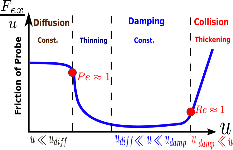
Figure 1: Sketch of the TTSP of thinning and thickening: the effective friction $\gamma_{eff}=F_{ex}/u$ vs. the pulling velocity $u$. Three time scales of bath particles are involved: diffusion, damping and single P-B collision, which lead to three friction behaviour: a high plateau regime, a low plateau regime, and an increasing friction regime, respectively. The pulling velocity controls the dominating time scales. The crossovers cause thinning and thickening. The turning points of thinning and thickening are around $Pe:=u/u_{diff}=\frac{R\gamma_{0}}{k_{B}T}u=1$ and $Re:=u/u_{damp}=\frac{m_{b}}{R\gamma_{0}}u=1$, respectively.

where $m_{b}$ is the mass of a bath particle; $\bm{v}_{i}$ is the velocity of the $i$-th bath particle, $\bm{u}$ is the fixed pulling velocity of the probe; $\gamma_{0}$ is the friction coefficient (all particles have the same value due to $\gamma_{0}\propto r_{0}\eta$; $\eta$ is the solvent’s viscosity.); $\bm{\xi}_{k}$ ($k=i$ or $p$) is a Gaussian random force satisfying the fluctuation-dissipation relation $\big{\langle}\xi_{k}^{\nu}(t)\xi_{k^{\prime}}^{\mu}(t^{\prime})\big{\rangle}=2\gamma_{0}k_{B}T\delta_{k,k^{\prime}}\delta^{\nu,\mu}\delta(t-t^{\prime})$ $\,\big{(}\nu,\mu\in\{x,y\}$ are the components of the random force$\big{)}$; $\bm{F}_{i,col}$ (or $\bm{F}_{p,col}$) is the interaction force between particles; $\bm{F}_{ex}$ is the external pulling force on the probe only.

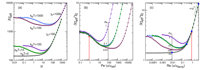
Figure 2: (a) Simulation results for the increased friction $\Delta\gamma_{eff}$ vs. the pulling velocity $u$ for different solvent frictions and temperatures. Different colors in (b) and (c) indicate different solvent frictions and temperatures as these labelled in (a).     (b) The rescaled increased friction $\Delta\gamma_{eff}/\gamma_{0}$ vs. the Peclet number $Pe=u/u_{diff}=\frac{R\gamma_{0}}{k_{B}T}u$. The red arrow indicates the turning point of the thinning around $Pe=1$. At $Pe=100$, for different solvent frictions and temperatures, the corresponding value of the Re numbers are indicated.     (c) The rescaled increased friction $\Delta\gamma_{eff}/\gamma_{0}$ vs. the Reynolds number $Re=u/u_{damp}=\frac{m_{b}}{R\gamma_{0}}u$. The red arrow indicates the turning point of the thickening around $Re=1$. At $Re=100$, for different solvent frictions and temperatures, the corresponding value of the Pe numbers are indicated. On the plot of $\{\gamma_{0}=100,\,k_{B}T=0\}$, four filled blue circles at $Re=0.01,\,0.3,\,1,\,5$ are drawn to compare with the corresponding streamlines in fig. 5.

According to the equation of motion (EOM) (1b), the probe’s increased friction $\Delta\gamma_{eff}:=\gamma_{eff}-\gamma_{0}$ is

$$\Delta\gamma_{eff}=\big{\langle}F_{p,col}\big{\rangle}/u,$$ (2)

where $u,F_{ex},F_{p,col}$ are absolute values of the corresponding vectors, and the random force has been averaged out: $\big{\langle}\bm{\eta}_{p}\big{\rangle}=0$.

Obviously, the P-B interaction directly leads to the increased friction, while the bath-bath (B-B) particle interaction affects indirectly. We omit the B-B interaction in our model because 1) such interaction may not be necessary for thinning and thickening behaviour; 2) the omission itself should be valid in the low density limit. In addition, we set the mass of the probe as much heavier than the mass of a bath particle: $m_{p}\gg m_{b}$, so that in the coordinate of the probe, P-B collision just causes specular reflection of the bath particles, but affects little the probe’s velocity.

Now the system of pulling a probe with fixed velocity $\bm{u}$ is equivalent to the system of a flow with velocity $-\bm{u}$ of a suspension of $N$ non-interacting bath particles passing a fixed disk with radius $R=2r_{0}$. The EOM of a bath particle (the index $i$ is dropped) in the coordinate of the probe is

$$m_{b}\dot{\bm{v}}=-\gamma_{0}(\bm{v}+\bm{u})+\bm{\xi}$$ (3a)

with the reflecting boundary condition (RBC)

$$\bm{v}=\bm{v}-(\bm{v}\cdot\bm{e}_{n})\bm{e}_{n}\,\mbox{ for }|\bm{r}|=R,$$ (3b)

where $R=2r_{0}$ is the contact distance between the probe and a bath particle, and $\bm{e}_{n}$ is the unit normal vector along the direction from the center of the probe to that of the bath particle colliding with it. Note that the P-B interaction term $\bm{F}_{i,col}$ in Eq.(1a) is mapped into the RBC (3b).

Being equivalent to its stochastic description Eq.(3), the probability description of a bath particle obeys the Fokker-Planck equation (FPE)

$$\partial_{t}P(\bm{r},\bm{v},t)=-\bm{v}\cdot\partial_{r}P+\frac{\gamma_{0}}{m_{b}}\partial_{\bm{v}}\cdot\Big{[}(\bm{v}+\bm{u})+\frac{k_{B}T}{m_{b}}\partial_{\bm{v}}\Big{]}P,$$ (4a)

which can be obtained by Kramers-Moyal expansion [28] of Eq. (3a). The corresponding RBC is

$$P(\bm{r},\bm{v},t)=P(\bm{r},\bm{v}-(\bm{v}\cdot\bm{e}_{n})\bm{e}_{n},t)\mbox{ for }|\bm{r}|=R.$$ (4b)

In principle, the steady state equation ($\partial_{t}P=0$) of the FPE (4a) can be solved with the RBC (4b). Then one can obtain the average collision force of $N$ bath particles on the probe:

$$\begin{split}\big{\langle}\bm{F}_{p,col}\big{\rangle}=\int d\bm{v}\oint_{r=R}dl&NP_{st}(\bm{r},\bm{v})\bm{v}\cdot(-\bm{e}_{n})\Theta[\bm{v}\cdot(-\bm{e}_{n})]\\ &2(-\bm{e}_{n})m_{b}\bm{v}\cdot(-\bm{e}_{n})\end{split}$$ (5)

where $P_{st}$ denotes the steady distribution, $dlNP_{st}(\bm{r},\bm{v})\bm{v}\cdot(-\bm{e}_{n})\Theta[\bm{v}\cdot(-\bm{e}_{n})]$ is the density current of bath particles with velocity $\bm{v}$ passing through a small contact surface $dl\bm{e}_{n}$ ( $\Theta(x)=1$ for $x\geq 0$;$\Theta(x)=0$ for $x\leq 0$ ), and $2(-\bm{e}_{n})m_{b}\bm{v}\cdot(-\bm{e}_{n})$ is the bath particles’ momentum transferred to the probe due to single P-B collision. Inserting Eq.(5) into Eq.(2), one obtains the effective friction $\gamma_{eff}$.

In practice, however, to analytically solve the FPE (4) is difficult due to the RBC (4b). Our strategy is to numerically solve Eq.(4) by simulation of the stochastic process Eq.(3), because of its equivalence to the FPE (4) and simplicity.

4 Stochastic Simulation

To calculate the effective friction, the stochastic dynamics simulation according to Eq.(3) is performed. The discrete form of the Gaussian random force is $\bm{\xi}=\sqrt{2\gamma_{0}k_{B}T/h}(\xi_{0}^{x},\xi_{0}^{y})$, where $\xi_{0}^{\mu}$ ($\mu\in{x,y}$) is the standard Gaussian random number of the probability distribution function as $P(\xi_{0}^{\mu})=\frac{1}{\sqrt{2\pi}}\exp(-\frac{\xi_{0}^{\mu\,2}}{2})$, and $h$ is the time step of the dynamics set to be $h=\frac{1}{2\gamma_{0}}$ for different solvent frictions. The box size is set to be $Lx\times Ly=20R\times 20R$ with periodic boundary conditions, which is large enough to suppress finite size effects. The mass of bath particles and the P-B contact distance are set to be unit values: $m_{p}=1$, $R=1$. The density of bath particles is also rescaled to unit value $n_{0}=1$, since it is not a control parameter in our model due to the assumption of non-interacting of bath particles. The control parameters are the pulling velocity $u$, the solvent friction $\gamma_{0}$ and the temperature $k_{B}T$, which are applied to investigate the whole regime of different time scales.

Initially, bath particles are homogeneously distributed in space with Maxwellian distributed velocities. Then the probe is pulled along the x direction with total running time $10R/u$, which ensures that the bath particles around the probe reach the steady state. After a transient time, the steady average P-B collision force is computed by detecting the bath particles passing through the boundary: $\big{\langle}\bm{F}_{p,col}\big{\rangle}=\frac{1}{\Delta t}\oint_{r=R}dl\int_{0}^{\Delta t}dt2\big{[}m_{p}(-\bm{e}_{n})\bm{v}(t)\cdot(-\bm{e}_{n})\big{]}\Theta[\bm{v}(t)\cdot(-\bm{e}_{n})]$, which is the simulation realization of the collision force expressed in Eq. (5). The corresponding increased friction $\Delta\gamma_{eff}$ is obtained based on Eq. (2).

5 Result

Fig. 2 (a) shows the simulation result of the increased friction $\Delta\gamma_{eff}$ versus the pulling velocity $u$ for different solvent frictions and temperatures, $\{\gamma_{0}=1000,\,k_{B}T=1000,100\}$ and $\{\gamma_{0}=100,\,k_{B}T=100,10,0\}$. All plots, except for $\{\gamma_{0}=100,\,k_{B}T=0\}$, exhibit linear response, thinning and thickening as expected by the TTSP. For the exception, only linear response and thickening occur, because no diffusion but only damping and collision time scales are involved.

Fig. 2 (b) shows that the rescaled increased friction $\Delta\gamma_{eff}/\gamma_{0}$ versus Peclet number, $Pe=u/u_{diff}=\frac{R\gamma_{0}}{k_{B}T}u$. In the small Pe regime $Pe<1$, the diffusion time scale dominates, all plots coincide with each other in a plateau value. With increasing $Pe$, diffusion becomes less important, all plots start to decrease around $Pe=1$, which agrees with the TTSP. Between $Pe=100$ and $Pe=1000$, for $\{\gamma_{0}=1000,\,k_{B}T=100\}$, the brown line, clearly there is a second plateau lower than the first one, being consistent with the TTSP. In addition, the length of the thinning regime varies for different data sets , because for the same $Pe$, the $Re$ numbers can also be different. At $Pe=100$, for $\{\gamma_{0}=1000,\,k_{B}T=100\}$, $Re=0.01$, bath particles are still in the damping regime; for $\{\gamma_{0}=100,\,k_{B}T=100\}$, $Re=1$, bath particles are already in the inertia (thickening) regime, which suppresses the thinning process.

Fig. 2 (c) shows that the rescaled increased friction $\Delta\gamma_{eff}/\gamma_{0}$ versus Reynolds number, $Re=u/u_{damp}=\frac{m_{b}}{R\gamma_{0}}u$. All plots start to converge around $Re=1$, which agrees with the TTSP. In the small $Re$ regime, for different plots, at $Re=0.01$, the frictions increase with the decreasing $Pe$ as indicated in the figure, which supports the TTSP that the diffusion causing larger friction than the one in the damping only regime $Pe\rightarrow\infty$. For $Re>1$, i.e. the inertia regime, all plots coincide with each other and asymptotically tend to $\Delta\gamma_{eff}\propto u$, because the flux of bath particles passing through the P-B contact surface is $j\propto n_{0}u$ with momentum transferring to the probe $p\propto mu$, and $\Delta\gamma_{eff}=\big{\langle}F_{col}\big{\rangle}/u=jp/u\propto u$.

In summary, the friction behaviour of different dominating time scales and of the two turning points as shown in fig. 2, all agree quite well with the TTSP.

6 Microscopic picture

The TTSP is indicated by $Pe$ and $Re$. Microscopically, what happens in the different $Pe$ and $Re$ regimes?

6.1 density distribution

It is convenient to compare the behaviour of bath particles in different $Pe$ regimes by computing the pair distribution function $g(\bm{r})$, which is the normalized number density of bath particles in the coordinate of the probe $g(\bm{r})=n(\bm{r})/n_{0}=V\int d\bm{v}\,p(\bm{r},\bm{v})$ ($V$ is the volume of bath particles, here for 2d it is the area, $n_{0}=N/V$). Fig. 3 shows the simulation result $g(\bm{r})$ for different $Pe$ numbers. For small $Pe$ numbers $Pe=0.1,1$, bath particles are both built up in front and left behind of the probe, i.e. the diffusion dominating regime. As $Pe$ is quite large, $Pe=10,100$, only a thin layer of bath particles build in front but no particles left behind in a long tail region of the probe, which means that the diffusion is ignorable. The observation that diffusion dominates in the small $Pe$ and is unimportant in large $Pe$, is consistent with the TTSP.

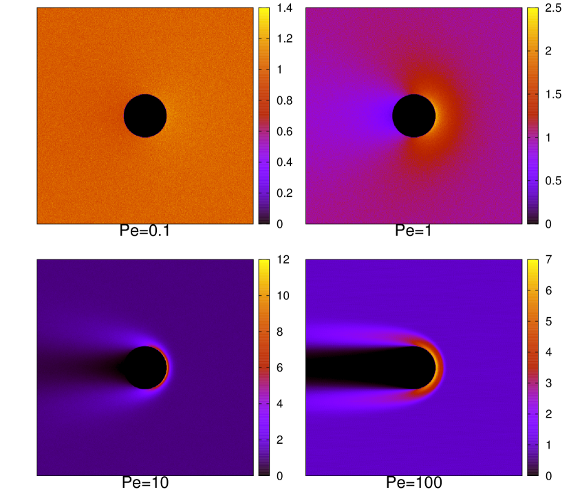
Figure 3: Pair distribution function $g(\bm{r})$ of bath particles in the frame of the probe for different Peclet numbers. The solvent friction is $\gamma_{0}=100$ and the temperature is $k_{B}T=100$.

6.2 velocity distribution

Does the pair distribution function contain enough information to calculate the effective friction? If the velocity of bath particles is Maxwellian distributed: $f_{eq}(\bm{v})=\big{(}\frac{1}{\sqrt{2\pi}v_{th}}\big{)}^{d}e^{-\frac{\bm{v}\cdot\bm{v}}{2v_{th}^{2}}}$ with thermal velocity $v_{th}=\sqrt{k_{B}T/m_{b}}$, then the total probability can be separated into $p(\bm{r},\bm{v})=V^{-1}g(\bm{r})f_{eq}(\bm{v})$, and the collision force in Eq. (5) is reduced to

$$\big{\langle}\bm{F}_{p,col}\big{\rangle}=-n_{0}k_{B}T\oint_{r=R}dl\bm{e}_{n}g(\bm{r}),$$ (6)

which is identical to the one in ref. [18]. If the velocity is delta distributed, $f(\bm{v})=\delta\big{(}\bm{v}-(-\bm{u})\big{)}$, the collision force in Eq. (5) is reduced to

$$\big{\langle}\bm{F}_{p,col}\big{\rangle}=-n_{0}2m_{b}\oint_{r=R}dl\bm{e}_{n}g(\bm{r})(\bm{u}\cdot\bm{e}_{n})^{2}\Theta[\bm{u}\cdot\bm{e}_{n}]$$ (7)

Inputting $g(\bm{r})$ from the simulation into Eq.(6) and Eq.(7), respectively, we obtain two increased effective frictions, the green line and black line, respectively, as indicated in fig. 4. Comparing them with the direct simulation result, the violet line (see fig. 4),

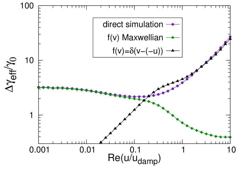
Figure 4: Increased effective friction from different methods: the violet line is the direct simulation result. the green and the black lines are calculated by inputting $g(\bm{r})$ from the simulation associated with Maxwellian distribution and delta distribution of velocity parts, respectively.

one can conclude that for the calculation of the friction, the pair distribution function still works, but the proper velocity distributions should be input, according to different $Re$ regimes: Maxwellian distribution in low Re and the delta distribution $\delta\big{(}\bm{v}-(-\bm{u})\big{)}$ in high Re.

6.3 streamline at $T=0$

To further investigate the role of the Reynolds number, let us consider the $T=0$ limit, where the diffusion time scale is ruled out, $Pe\rightarrow\infty$. Eq.(3a) is reduced to

$$m_{b}\dot{\bm{v}}=-\gamma_{0}\bm{v}-\gamma_{0}\bm{u}$$ (8)

with the RBC (3b). Interestingly, such simple dynamics provides a clear mechanism of thickening: the crossover from creep flow in the low Re to gas-like (inertial) flow in high Re, see fig. 5. The black curves are the streamlines of the bath particles in the frame of the probe; red arrows are the velocity field. Before any collision, bath particles are moving with a constant velocity $-\bm{u}$. Collision causes mirror-like reflection. The term $-\gamma_{0}\bm{v}$ reduces the velocity, while $-\gamma_{0}\bm{u}$ accelerates it. A loose criteria of single-collision-only should be $ut_{damp}\geq R$, i.e. $Re=u\frac{m_{b}}{R\gamma_{0}}\geq 1$. In the small $Re$ limit, many P-B collisions occur and the bath particles tend to creep along the surface, see fig. 5 $Re=0.01$, which causes $F_{col}\propto u$ and $\Delta\gamma_{eff}\propto u^{0}$(the proof will be given somewhere), while in the large Re limit, the single collision causes $F_{col}\propto u^{2}$ and $\Delta\gamma_{eff}\propto u^{1}$.

Based on the microscopic picture of $Re$ (fig. 5), we can also understand why Maxwellian distribution works in low Re but fails in high Re. Let us consider the $Pe\gg 1$ limit, where a bath particle moves with velocity $-\bm{u}$ relative to the probe before any P-B collision . $Re$ determines whether the solvent plays a role during P-B collisions. 1) If $Re\ll 1$, damping dominates, the injecting velocity $-\bm{u}$ of the bath particle is quickly ”erased” due to the damping and agitation processes by the solvent at the beginning of a few P-B collisions. In the following many times P-B collisions, the bath particle transfers the thermalized velocities to the probe. That’s why Maxwellian distribution works in this limit. b) If $Re\gg 1$, inertia dominates, the P-B collision happens once only. The bath particle’s velocity transferring to the probe is exactly the injecting velocity $-\bm{u}$, which has nothing to do with the solvent. Thus, instead of the Maxwellian, the delta distribution $\delta\big{(}\bm{v}-(-\bm{u})\big{)}$ works in this limit.

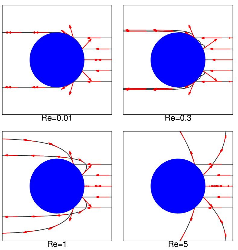
Figure 5: Streamlines of bath particles for different Reynolds numbers at the $T=0$ limit. Red arrows are the velocity field (rescaled by the pulling velocity for comparison). For small Reynolds number, the bath particles behave like creep flow around the contact surface. For high Reynolds number, they behave gas-like: single collision and flying away. The corresponding increased frictions are indicated with four filled blue circles in the gray line in fig. 2(c).

7 Conclusion

We propose a TTSP to unify thinning and thickening phenomena in active microrheology (see fig. 1), and confirm it by a model of pulling with fixed velocity. The simulation result (fig. 2), which is equivalent to the solution of the FPE (4) in steady state, shows linear response, thinning and thickening. As far as we know, this is the first example demonstrating that both thinning and thickening can occur in non-interacting bath particles systems (only P-B interaction is included), which indicates that the many body interaction is not necessary for thinning/thickening behaviour in the low density. Furthermore, as shown in fig. 2, the results of the turning points of the thinning and thickening being around $Pe=1$ and $Re=1$, respectively, and the friction behaviour in different time scale regimes, all agree with the TTSP.

Microscopically, the pair distribution function $g(\bm{r})$ is obtained from the simulation as shown in figs.3. For the calculation of the friction, we find that with the input $g(\bm{r})$ from the simulation, Maxwellian distribution works in low Re, but fails in high Re; while the delta distribution $\delta\big{(}\bm{v}-(-\bm{u})\big{)}$ works in high Re, but fails in low Re. In the T=0 limit ($Pe\rightarrow\infty$), we obtain a clear microscopic picture of thickening for different $Re$ regimes, see fig.5. When $Re\ll 1$, damping dominates, the constant friction comes from creep flow, the bath particles collide with the probe and then creep around it; when $Re\gg 1$, inertial dominates, the increasing friction comes from the single P-B collision. Based on the picture of bath particles in different $Re$ regimes, the validity/invalidity of Maxwellian distribution can also be understood.

According to the TTSP, thinning arises from the crossover from diffusion to damping, and thickening arises from the crossover from damping to inertia. Note that diffusion was not involved in the experiments of pulling a single particle in static ($T=0$) granular systems [23, 24], that’s why thinning was not observed. For the same reason, it was not included in our earlier kinetic model [26]. Thickening was not found in colloidal systems [14, 15, 16, 18, 19], because they were limited to $Re\ll 1$ regime, where inertia is unimportant.

The TTSP should also be valid in the high density with dressed values of $Pe$ and $Re$. B-B many body interaction increases the friction of a single bath particle, $\gamma^{\prime}_{0}>\gamma_{0}$ (in the low density limit, $\gamma^{\prime}_{0}$ is just the solvent friction $\gamma_{0}$). Based on the TTSP, the turning point of thinning $Pe=1\propto u\gamma^{\prime}_{0}$ should shift to a smaller pulling velocity value, and that of the thickening $Re=1\propto u/\gamma^{\prime}_{0}$ should shift to a larger value.

- [1] \NameSquires T. M. Mason T. G. \REVIEWAnnu. Rev. Fluid Mech.422010413.
- [2] \NamePuertas a. M. Voigtmann T. \REVIEWJ. Phys.: Condens. Matter262014243101.
- [3] \NameMason T. Weitz D. \REVIEWPhys. Rev. Lett.7419951250.
- [4] \NameWilson L. G. Poon W. C. K. \REVIEWPhys. Chem. Chem. Phys13201110617.
- [5] \NameCandelier R. Dauchot O. \REVIEWPhys. Rev. Lett.1032009128001.
- [6] \NameCoulais C., Seguin A. Dauchot O. \REVIEWPhys. Rev. Lett.1132014198001.
- [7] \NameR. Kubo, M. Toda N. H. \BookStatistical Physics II: Nonequilibrium Statistical Mechanics 2nd Edition (Springer) 2003.
- [8] \NameEvans D. J. Morriss G. P. \BookStatistical mechanics of nonequilibrium liquids 2nd Edition (Cambridge University Press) 2008.
- [9] \NameMarconi U. M. B., Puglisi A., Rondoni L. Vulpiani A. \REVIEWPhys. Rep.4612008111.
- [10] \NameSeifert U. \REVIEWRep. Prog. Phys.752012126001.
- [11] \NameSeto R., Mari R., Morris J. F. Denn M. M. \REVIEWPhys. Rev. Lett.1112013218301.
- [12] \NameWyart M. Cates M. \REVIEWPhys. Rev. Lett.112201498302.
- [13] \NameKawasaki T., Ikeda A. Berthier L. \REVIEWEurophys. Lett.107201428009.
- [14] \NameWilson L. G., Harrison a. W., Schofield a. B., Arlt J. Poon W. C. K. \REVIEWJ. Phys. Chem. B11320093806.
- [15] \NameGomez-Solano J. R. Bechinger C. \REVIEWEurophys. Lett.108201454008.
- [16] \NameCarpen I. C. Brady J. F. \REVIEWJ. Rheol.4920051483.
- [17] \NameWinter D., Horbach J., Virnau P. Binder K. \REVIEWPhys. Rev. Lett.1082012028303.
- [18] \NameSquires T. M. Brady J. F. \REVIEWPhys. Fluid172005073101.
- [19] \NameReinhardt J., Scacchi A. Brader J. M. \REVIEWJ. Chem. Phys.1402014.
- [20] \NameGazuz I., Puertas a. M., Voigtmann T. Fuchs M. \REVIEWPhys. Rev. Lett.1022009248302.
- [21] \NameGazuz I. Fuchs M. \REVIEWPhys. Rev. E872013032304.
- [22] \NameGnann M. V., Gazuz I., Puertas a. M., Fuchs M. Voigtmann T. \REVIEWSoft Matter720111390.
- [23] \NameTakehara Y., Fujimoto S. Okumura K. \REVIEWEurophys. Lett.92201044003.
- [24] \NameTakehara Y. Okumura K. \REVIEWPhys. Rev. Lett.1122014148001.
- [25] \NameFiege A., Grob M. Zippelius A. \REVIEWGranular Matter142012247.
- [26] \NameWang T., Grob M., Zippelius A. Sperl M. \REVIEWPhys. Rev. E892014042209.
- [27] \NameSwan J. W. Zia R. N. \REVIEWPhys. Fluid252013083303.
- [28] \NameRisken H. \BookThe Fokker-Planck equation : methods of solution and applications (Springer) 1989.