Arecibo Pulsar Survey Using ALFA. IV. Mock Spectrometer Data Analysis, Survey Sensitivity, and the Discovery of 41 Pulsars

Abstract

The on-going PALFA survey at the Arecibo Observatory began in 2004 and is searching for radio pulsars in the Galactic plane at 1.4 GHz. Observations since 2009 have been made with new wider-bandwidth spectrometers than were previously employed in this survey. A new data reduction pipeline has been in place since mid-2011 which consists of standard methods using dedispersion, searches for accelerated periodic sources, and search for single pulses, as well as new interference-excision strategies and candidate selection heuristics. This pipeline has been used to discover 41 pulsars, including 8 millisecond pulsars (MSPs; $P<10$ ms), bringing the PALFA survey’s discovery totals to 145 pulsars, including 17 MSPs, and one Fast Radio Burst (FRB). The pipeline presented here has also re-detected 188 previously known pulsars including 60 found in PALFA data by re-analyzing observations previously searched by other pipelines. A comprehensive description of the survey sensitivity, including the effect of interference and red noise, has been determined using synthetic pulsar signals with various parameters and amplitudes injected into real survey observations and subsequently recovered with the data reduction pipeline. We have confirmed that the PALFA survey achieves the sensitivity to MSPs predicted by theoretical models. However, we also find that compared to theoretical survey sensitivity models commonly used there is a degradation in sensitivity to pulsars with periods $P\stackrel{{\scriptstyle>}}{{{}_{\sim}}}100$ ms that gradually becomes up to a factor of $\sim$ 10 worse for $P>4$ s at $\mathrm{DM}<150$ $\mathrm{pc\,cm^{-3}}$. This degradation of sensitivity at long periods is largely due to red noise. We find that $35\pm 3$ % of pulsars are missed despite being bright enough to be detected in the absence of red noise. This reduced sensitivity could have implications on estimates of the number of long-period pulsars in the Galaxy.

1. Introduction

Pulsars are rapidly rotating, highly magnetized neutron stars, the remnants of massive stars after their death in supernova explosions. They are extremely valuable astronomical tools with many physical applications that have been used to, for example, constrain the equation of state of ultra-dense matter (e.g. Hessels et al., 2006; Demorest et al., 2010), test relativistic gravity (e.g Kramer et al., 2006b; Antoniadis et al., 2013), probe plasma physics within the magnetosphere (e.g. Hankins et al., 2003; Kramer et al., 2006a; Lyne et al., 2010; Hermsen et al., 2013), and gain a better understanding of the complete radio pulsar population (e.g. Faucher-Giguère & Kaspi, 2006). Certain individual pulsar systems are especially well suited to studying these areas of astrophysics, and thus continued pulsar surveys to find these rare objects remain a major scientific driver in the field.

Radio pulsars are found primarily in non-targeted, wide-area surveys such as the Pulsar-ALFA (PALFA) survey at 1.4 GHz, which began in 2004 (Cordes et al., 2006). PALFA observations use the 7-beam Arecibo L-band Feed Array (ALFA) receiver of the Arecibo Observatory William E. Gordon 305-m Telescope and focus on the Galactic plane ($|b|<5$^∘) in the two regions visible with Arecibo, namely the “inner Galaxy” region (32^∘ $\stackrel{{\scriptstyle<}}{{{}_{\sim}}}$ $l$ $\stackrel{{\scriptstyle<}}{{{}_{\sim}}}$ 77^∘), and the “outer Galaxy” region (168^∘ $\stackrel{{\scriptstyle<}}{{{}_{\sim}}}$ $l$ $\stackrel{{\scriptstyle<}}{{{}_{\sim}}}$ 214^∘).

For the first 5 years, PALFA survey observations were made using the Wideband Arecibo Pulsar Processor (WAPP), a 3-level auto-correlation spectrometer with 100 MHz of bandwidth (Dowd et al., 2000). Since 2009, the Mock spectrometer, a 16-bit poly-phase filterbank with 322 MHz of bandwidth, has replaced the WAPP spectrometer as the data-recorder of the PALFA survey. The increased bandwidth, poly-phase filterbank design, and increased bit-depth of the Mock spectrometer have increased the sensitivity and robustness to interference of the PALFA survey. For this reason, we are re-observing regions of the sky previously observed with the WAPP spectrometers.

The PALFA consortium currently employs two independent full-resolution data analysis pipelines. The Einstein@Home-based pipeline (E@H) has already been described by Allen et al. (2013): this pipeline derives its computational power by aggregating the spare cycles of a global network of PCs and mobile devices using the BOINC platform, and is also searching data from the PALFA survey for pulsars. In this work we describe the pipeline based on the PRESTO suite of pulsar search programs (Ransom, 2001). In addition to these pipelines, we also employ a reduced-resolution “Quicklook” pipeline, which is run on-site at Arecibo shortly after observing sessions are complete and which enables a more rapid discovery and confirmation of strong pulsars (Stovall, 2013).

As of March 2015, there have been 145 pulsars discovered in WAPP and Mock spectrometer observations with the various PALFA data analysis pipelines. This is already a sizable increase on the known sample of 258 Galactic radio pulsars in the full survey region found in other searches.

The relatively high observing frequency and unparalleled sensitivity of Arecibo, coupled with the high time and frequency resolution of PALFA ($\tau_{\mathrm{samp}}\simeq\!65.5\,\mu$s and $\Delta f_{\mathrm{chan}}\simeq\!336$ kHz, respectively) make it particularly well suited for detecting millisecond pulsars (MSPs) deep in the plane of the Galaxy, such as the distant MSPs reported by Crawford et al. (2012) and Scholz et al. (2015), the highly eccentric MSP PSR J1903+0327 (Champion et al., 2008), and faint, young pulsars (e.g. Hessels et al., 2008). The huge instantaneous sensitivity of Arecibo enables short integration times, which has been helpful in detecting relativistic binaries (e.g. PSR J1906+0746; Lorimer et al., 2006a) by reducing the deleterious effect of time-varying Doppler shifts of binary pulsars. The PALFA survey has also proven successful at detecting transient astronomical signals. For example, the survey has led to the discovery of several Rotating Radio Transient pulsars (RRATs; Deneva et al., 2009), as well as FRB 121102, the first Fast Radio Burst (FRB) detected with a telescope other than the Parkes Radio Telescope (Spitler et al., 2014).

While PALFA is the most sensitive large-scale survey for radio pulsars ever conducted, it is not the only on-going radio pulsar survey. Other major surveys are the HTRU-S (Keith et al., 2010), HTRU-N (Barr et al., 2013), and SPAN512 (Desvignes et al., 2013) surveys at $\sim$ 1.4 GHz, the GBNCC (Stovall et al., 2014) and AO327 drift (Deneva et al., 2013) surveys at $\sim$ 350 MHz, and the LOFAR surveys (Coenen et al., 2014) at $\sim$ 150 MHz.

The underlying distributions of the pulsar population can be estimated using simulation techniques (e.g. Lorimer et al., 2006b; Faucher-Giguère & Kaspi, 2006). The large sample of pulsars found in non-targeted surveys are essential for these simulations. However, for population analyses to be done accurately, the selection biases of each survey must be taken into account. While the sensitivity of pulsar search algorithms is reasonably well understood, the effect of radio frequency interference (RFI) on pulsar detectability has not been previously studied in detail.

This paper reports on the current state of PALFA’s primary search pipeline, its discoveries, and its sensitivity. The rest of the article is organized as follows: the observing set-up is summarized in § 2. The details of the PALFA PRESTO-based pipeline are described in § 3. § 4 reports basic parameters of the pulsars found with the pipeline, and § 5 details how the survey sensitivity is determined, including a technique involving injecting synthetic pulsars into the data. These accurate sensitivity limits are used to improve upon population synthesis analyses in §6. The broader implications of the accurate determination of the survey sensitivity are presented in § 7 before the paper is summarized in § 8.

2. Observations

The PALFA survey observations have been restricted to the two regions of the Galactic plane ($|b|<5$^∘) visible from the Arecibo observatory, the inner Galaxy (32^∘ $\stackrel{{\scriptstyle<}}{{{}_{\sim}}}$ $l$ $\stackrel{{\scriptstyle<}}{{{}_{\sim}}}$ 77^∘), and the outer Galaxy (168^∘ $\stackrel{{\scriptstyle<}}{{{}_{\sim}}}$ $l$ $\stackrel{{\scriptstyle<}}{{{}_{\sim}}}$ 214^∘). Integration times are 268 s and 180 s for inner and outer Galaxy observations, respectively.

To optimize the use of telescope resources, the PALFA survey operates in tandem with other compatible projects using the ALFA 7-beam receiver. In particular, we have reciprocal data-sharing agreements with collaborations that search for galaxies in the optically obscured (“zone of avoidance”) directions through the Milky Way (Henning et al., 2010) and recombination-line studies of ionized gas in the Milky Way (Liu et al., 2013). The PALFA project leads inner Galaxy observing sessions, whereas our partners lead outer Galaxy sessions.

For the inner Galaxy region, the pointing strategy has prioritized observations of the $|b|<2$^∘ region before densely sampling the Galactic plane at larger Galactic latitudes. To densely cover a patch of sky out to the ALFA beam FWHM, three interleaved ALFA pointings are required (see Cordes et al., 2006, for more details). In contrast, our commensal partners have focused outer Galaxy observations in order to densely sample particular Galactic longitude/latitude ranges. A sky map showing the observed pointing positions can be found in Figure 1.

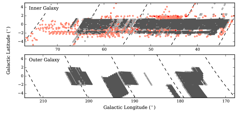
Figure 1.— Sky map showing the locations of PALFA observations with the Mock spectrometers, which began in 2009, for the inner and outer Galaxy regions. Each position plotted represents the center of the 3-pointing set required to densely sample the area. Positions that have been only sparsely observed (i.e. 1 of 3 pointing positions observed) are indicated with un-filled circles. Positions with 2 of 3 pointings observed are indicated with a light-colored filled circle. Positions that have been densely observed (i.e. all 3 pointing positions observed) are indicated with dark-colored filled circles. Red indicates observations made prior to adjusting our pointing grid at the request of our commensal partners. As a result, some of the sky area covered in early Mock observations has not been re-observed using the Mocks and the current commensal pointing grid.

Observations conducted with ALFA have a bandwidth of 322 MHz centered at 1375 MHz. Each of the seven ALFA beams is split into two overlapping 172-MHz sub-bands and processed independently by the Mock spectrometers. The sub-bands are divided into 512 channels, each sampled every $\sim$65.5 $\mu$s. The observing parameters are summarized in Table 1. The data are recorded to disk in 16-bit search-mode PSRFITS format (Hotan et al., 2004).

PALFA survey data have been recorded with the Mock spectrometers since 2009. Although, in 2011 our pointing grid was altered slightly to accommodate our commensal partners. This required some sky positions to be re-observed. Prior to 2009, survey observations were recorded with the Wideband Arecibo Pulsar Processors (WAPPs; see Dowd et al., 2000; Cordes et al., 2006). The two data recording systems were run in parallel during 2009 to check the consistency and quality of the Mock spectrometer data.

An unpulsed calibration diode is fired during the first (or sometimes last) 5–10 s of our integration. While this is primarily used by our partners, we have found the diode signals useful in calibrating observations for our sensitivity analysis (see § 5.4). The calibration signal is removed from the data prior to searching (see § 3.2).

The original 16-bit Mock data files are compressed to have 4 bits per sample. These smaller data files are more efficient to ship and analyze thanks to reduced disk-space requirements. The 4-bit data files utilize the scales and offsets fields of the PSRFITS format to retain information about the bandpass shape despite the reduced dynamic range. The scales and offsets are computed and stored for every 1-s sub-integration. This reduction of bit-depth results in a total loss of only a few percent in the $S/N$ of pulsar signals.

The converted 4-bit PSRFITS data files are copied to hard disks, and couriered from Arecibo to Cornell University where they are archived at the Cornell University Center for Advanced Computing. Meta-data about each observation, parsed from the telescope logs and the file headers, are stored in a dedicated database.

As of 2014 November, a total of 87689 beams of Mock spectrometer data have been archived. The break-down of observed, archived and analyzed sky positions for the two survey regions is shown in Table 2.

PALFA observations more than one year old are publicly available. Small quantities of data can be requested via the web. Access to larger amounts of data is also possible, but must be coordinated with the collaboration because of logistics.

Additional details about the data management logistics and data preparation are in §§ 3.1 and 3.2.

3. Pulsar and Transient Search Pipeline

The PRESTO-based pipeline has been used to search PALFA observations taken with the Mock spectrometers since mid-2011 for radio pulsars and transients. All processing is done using the Guillimin supercomputer of McGill University’s High Performance Computing center.

While the pipeline described here was designed specifically for the PALFA survey, it is sufficiently flexible to serve as a base for the data reduction pipeline of other surveys. For example, the SPAN512 survey being undertaken at the Nançay Radio Telescope uses a version of the PALFA PRESTO pipeline described here tuned to their specific needs (Desvignes et al., 2013). The PALFA pipeline source code is publicly available online.

Since the analysis began with the pipeline, there have been several major improvements, primarily focusing on ameliorating its robustness in the presence of RFI (§ 3.4), as well as post-processing algorithms for identifying the best pulsar candidates (§ 3.5). The PALFA consortium is constantly monitoring the performance of the pipeline and the RFI environment at Arecibo (as described later, RFI is one of the major challenges), and looking for ways to further improve the analysis. Here we report on the state of the software as of early-2015.

The pipeline overview presented here is grouped into logical components. In § 3.1 we outline the significant data tracking and processing logistics required to automate the analysis. In § 3.2 we detail the data file preparation required before searching an observation. In § 3.3 we describe the techniques used to search for periodic and impulsive pulsar signals. In § 3.4 we summarize the various complementary stages of RFI identification and mitigation. Finally, in §§ 3.5 and 3.6 we outline the tools used to help select and view pulsar candidates, as well as other on-line collaborative facilities used by the PALFA consortium.

Figure 2 shows a flowchart summarizing the stages of the pipeline.

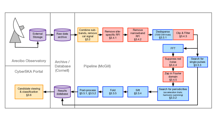
Figure 2.— An overview of the PALFA survey’s PRESTO-based pipeline. The color of each element reflects the category of the step: searching is blue; RFI mitigation is red; data storage and databases are purple; miscellaneous processes are yellow. Additional details about each pipeline stage can be found in the sections listed in each box.

3.1. Logistics

The PALFA search pipeline is designed to be almost entirely automated. This includes the logistics of data management required to maintain the analysis of $\sim 1000$ observations on the Guillimin supercomputer at any given time. This is accomplished with a job-tracker database that maintains the status of processes that are downloading raw data, reducing data, and uploading results.

The pipeline is configured to continually request and download raw data that have not been processed and delete the local copies of files that have been successfully analyzed. Data files are copied to McGill via FTP from the Cornell University Center for Advanced Computing (CAC). The multi-threaded data transfers from the CAC to McGill are sufficiently fast to maintain 1000–2000 jobs running simultaneously.

When the transfer of an observation is complete, job entries are created in the pipeline’s job-tracker database. As compute resources become available, jobs are automatically submitted to the super-computer’s queue.

When jobs terminate, the pipeline checks for results and errors. Failed jobs are automatically re-submitted up to three times to allow for occasional hiccups of the Guillimin task management system, or processing node glitches. If all three processing attempts result in failure, the observation is flagged to be dealt with manually. Observations that are salvageable are re-processed after fixes are applied. The positions of un-salvageable observations are re-inserted into the observing schedule, along with those from observations severely contaminated with RFI. Observations may be un-salvageable if they are aborted scans, contain malformed metadata, or their files have become corrupted. Only $\sim$ 0.15% of all observations have data files that cannot be searched, and only $\sim$ 4.5% of all observations are flagged to be re-observed due to excessive RFI.

The results from successfully processed jobs are parsed and uploaded to a database at the CAC, and the local copies of the data files are removed to liberate disk space enabling more observations to be requested, downloaded, and analyzed.

The inspection of uploaded results is done with the aid of a web-application (see §3.6).

3.2. Pre-processing

Before analyzing the data for astrophysical signals, the two Mock sub-bands must be combined into a single PSRFITS file. Each of the two Mock data files have 512 frequency channels, 66 of which are overlapping with the other file. For each sub-integration of the observation, the 478 low-frequency channels from the bottom sub-band and the 480 high-frequency channels from the top sub-band are extracted, concatenated together – along with two extra, empty frequency channels – for each sample, and written into a new full-band data file, consisting of 960 channels. The choice to discard part of both bands was made in order to mitigate the effect of the reduced sensitivity at the extremities of the Mock sub-bands, which causes a slight reduction of sensitivity where they are joined together.

The PSRFITS scales and offsets of the Mock sub-bands are adjusted such that the data value levels of top and bottom bands are appropriately weighted with respect to each other.

The combining of the two Mock sub-bands is performed using combine_mocks of psrfits_utils .

Next, the sub-integrations containing the calibration diode signal are deleted from the observation. The start time and length of the observation are updated accordingly.

At this stage, prior to searching for periodic and impulsive signals, PRESTO’s rfifind is run on the merged observation to generate an RFI mask. See § 3.4.2 for details.

3.3. Searching Components

We will now cover the various steps required to search for pulsars and transients.

3.3.1 Dedispersion

Because the DMs of yet-undiscovered pulsars and transients are not known in advance, a wide range of trial DMs must be used to maintain sensitivity to pulsars. For each trial DM value a dedispersed time series is produced by shifting the frequency channels according to the assumed DM value and then summing over frequency. When generating these time series, the motion of the Earth around the Sun is removed so that the data are referenced to the Solar System barycenter, assuming the coordinates of the beam center.

The PALFA PRESTO pipeline searches observations for periodic and impulsive signals up to a DM of $\sim$ 10000 $\mathrm{pc\,cm^{-3}}$. We search to such high DMs despite the maximum DM in our survey region predicted by the NE2001 model being $\sim$ 1350 $\mathrm{pc\,cm^{-3}}$ (Cordes & Lazio, 2002) to ensure sensitivity to highly-dispersed, potentially extragalactic FRBs (e.g. Thornton et al., 2013; Spitler et al., 2014).

A dedispersion plan is determined by balancing the various contributions to pulse broadening that can be controlled: the duration of each sample (including down-sampling), $\tau_{\mathrm{samp}}$; the dispersive smearing within a single channel, $\tau_{\mathrm{chan}}$; the dispersive smearing within a single sub-band due to approximating the DM, $\tau_{\mathrm{sub}}$; and the dispersive smearing across the entire observing band due to the finite DM step size (i.e. if the DM of the pulsar is half-way between two DM trials), $\tau_{\mathrm{BW}}$. Additionally, pulses are broadened by interstellar scattering, $\tau_{\mathrm{scatt}}$, which cannot be removed. The amount of scatter-broadening depends on the DM, observing frequency and line-of-sight. Cordes (2002) empirically determined the relationship as

$$\log\tau_{\mathrm{scatt}}= - 3.59+0.129\log\mathrm{DM}$$ (1)

$$+ 1.02\left(\log\mathrm{DM}\right)^{2}-4.4\log\nu,$$

where $\tau_{\mathrm{scatt}}$ is given in $\mu$s, and $\nu$ is the observing frequency in GHz. Even for the same DM, $\log\tau_{\mathrm{scatt}}$ are different for pulsars in different locations with a standard deviation of $\sigma=0.65$ (Cordes, 2002). Because $\tau_{\mathrm{scatt}}$ cannot (in practice) be corrected, we ignore it when determining our dedispersion plan.

The total correctable pulse broadening, $\tau_{\mathrm{tot}}$, is estimated by summing the first four contributions in quadrature,

$$\tau_{\mathrm{tot}}=\sqrt{\tau_{\mathrm{samp}}^{2}+\tau_{\mathrm{chan}}^{2}+\tau_{\mathrm{sub}}^{2}+\tau_{\mathrm{BW}}^{2}}.$$ (2)

All of these broadening terms vary with DM. The dedispersion plan is chosen to equate these four broadening effects roughly by adjusting the DM step-size and down-sampling factor as a function of DM. To reduce the number of DM trials, the step-size is never so small that $\tau_{\mathrm{BW}}\stackrel{{\scriptstyle<}}{{{}_{\sim}}}0.1$ ms.

The PALFA survey dedispersion plan for Mock spectrometer data was determined with a version of PRESTO’s DDplan.py modified to allow for non-power-of-two down-sampling factors, and is shown in Table 3. The down-sampling factors are selected to be divisors of the number of spectra per sub-integration, 15270. The amount of dispersive smearing incurred at the middle of the observing band, $\sim$ 1375 MHz, when using the dedispersion plan in Table 3, ranges from $\sim$ 0.1 ms for the lowest DMs, to $\sim$ 1 ms for DMs of a few 100 $\mathrm{pc\,cm^{-3}}$, increasing to $\sim$ 10 ms for a DM of $\sim$ 10000 $\mathrm{pc\,cm^{-3}}$. Above a DM of $\sim$ 500 $\mathrm{pc\,cm^{-3}}$ scattering begins to dominate (see Fig. 3).

The more aggressive down-sampling at higher DMs has the advantage of reducing the data size, making the analysis more efficient. Also, at higher DMs the step-size between successive DM trials is increased, further reducing the amount of processing. Therefore, the extra computing required to go to high DMs is relatively small compared to what is required to search for pulsars and transients at low DMs. Searching DMs between 1000 $\mathrm{pc\,cm^{-3}}$ and 10000 $\mathrm{pc\,cm^{-3}}$ adds only $\sim$ 5 % the total data analysis time.

Dedispersion is done with PRESTO’s prepsubband, passing through the raw data 99 times, and resulting in 7292 dedispersed time series. In all cases prepsubband internally uses 96 sub-bands, each of 10 MHz, for its two-stage sub-band dedispersion process. Time intervals containing strong impulsive RFI are removed by prepsubband, as prescribed by a RFI mask (see § 3.4.2).

A second set of dedispersed time series are created as before, but also applying a version of the zero-DM filtering technique described by Eatough et al. (2009) that has been augmented to use the bandpass shape when removing the zero-DM signal from each channel. These zero-DM filtered time series are especially useful for single-pulse searching, which is described in § 3.3.3. See § 3.4.3 for details on time-domain RFI mitigation strategies used.

Dedispersion makes up roughly 15-20 % of the processing time.

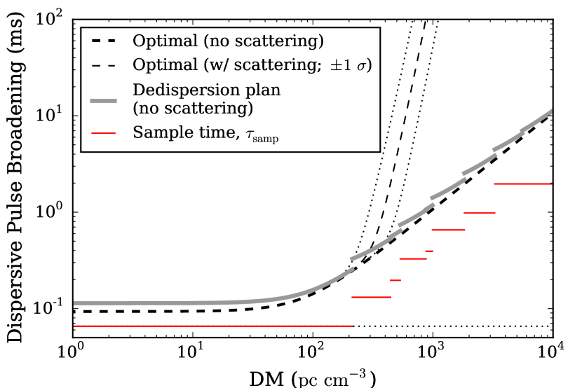
Figure 3.— Pulse broadening from down-sampling, and dispersive DM smearing for the dedispersion plan generated by DDplan.py shown in Table 3 (gray), as well as the optimal case (dashed black) where neither down-sampling nor smearing from DM errors are included. The optimal case including interstellar scattering is shown (with $\pm~{}1\sigma$; thin dashed black) assuming the empirical scattering dependence on DM of Cordes (2002). While this dependence is likely reasonable for estimating the scattering of Galactic sources, it is likely to grossly overestimate the scattering of extragalactic sources (e.g. FRBs). In all cases, the middle of the observing band is assumed ($\sim$ 1375 MHz). Discontinuities are due to down sampling. The horizontal lines (red) show the down sampled time resolution at various DMs.

3.3.2 Periodicity Searching

For every dedispersed time series, the discrete Fourier transform (DFT) is computed using PRESTO’s realfft. Prior to searching the DFT for peaks, it is normalized to have unit mean and variance. The normalization algorithm is designed mainly to suppress red noise (i.e. low-frequency trends in the time series; for more details see § 3.4.4). Also, Fourier bins likely to contain interference are replaced with the median-value of nearby bins. Details of the algorithm used to determine RFI-prone frequencies are described in § 3.4.5.

Two separate searches of the DFT are conducted using PRESTO’s accelsearch. Both searches identify peaks in the DFT down to a frequency of 0.125 Hz.

The first, zero-acceleration, search is tuned to identify isolated pulsars. The power spectrum of the signal from an isolated pulsar will consist of narrow peaks at the rotational frequency of the pulsar and at harmonically related frequencies. The number of significant harmonics depends on the width of the pulse profile, $W$, and the spin period, $P$, as $N_{\mathrm{harm}}\sim P/W$. To improve the significance of narrow signals, power from harmonics is summed with that of the fundamental frequency. The zero-acceleration search sums up to 16 harmonics, including the odd harmonics, in powers of 2 (i.e. 1, 2, 4, 8, 16 harmonics). This harmonic summing procedure also improves the precision of the detected frequency.

The second, high-acceleration search is optimized to find pulsars in binary systems. The time-varying line-of-sight velocity of such pulsars gives rise to a Doppler shift that varies over the course of an observation. This smears the signal over multiple bins in the Fourier domain. To recover sensitivity to binary pulsars we use the Fourier-domain acceleration search technique described in Ransom et al. (2002). In short, the high-acceleration search performs matched-filtering on the DFT using a series of templates each corresponding to a different constant acceleration. We search using templates up to 50 Fourier bins wide, which corresponds to a maximum acceleration of $\sim$ 1650 $\mathrm{m/s^{2}}$ for a 5-min observation of a 10-ms pulsar. Only up to 8 harmonics are summed in the high-acceleration case because of its larger computational requirements.

For each of the periodic signal candidates identified in both the zero- and high-acceleration searches we compute the equivalent Gaussian significance, $\sigma_{F}$, based on the probability of seeing a noise value with the same amount of incoherently summed power (see Ransom et al., 2002, for details). The zero- and high-acceleration candidate information is saved to separate lists for later post-processing (see § 3.3.4).

Typically, the zero-acceleration and high-acceleration searches make up between 2 %-5 % and $\sim$ 30 % of the overall computation time, respectively.

3.3.3 Single Pulse Searching

Each dedispersed time series is also searched with PRESTO’s single_pulse_search.py for impulsive signals with a matched-filtering technique (e.g. Cordes & McLaughlin, 2003). Multiple box-car templates corresponding to a range of durations up to 0.1 s are used. Candidate single-pulse events at least 5 times brighter than the standard deviation of nearby bins, $\sigma_{\mathrm{loc}}$, are recorded. Diagnostic plots featuring only $>$ 6 $\sigma_{\mathrm{loc}}$ candidate events are generated and archived for later viewing. In addition to the basic diagnostic plots, all of the $>$ 5 $\sigma_{\mathrm{loc}}$ events are used in post-processing algorithms designed to distinguish astrophysical signals (e.g. from pulsars/RRATs and extragalactic FRBs) from RFI and noise. The algorithms employed by PALFA are described elsewhere (Spitler, 2013; Karako-Argaman et al., 2015).

The same searching and post-processing procedure is also applied to data from which the DM=0 $\mathrm{pc\,cm^{-3}}$ time series has been subtracted, using an enhanced version of what was originally described in Eatough et al. (2009). See § 3.4.3 for more details about the time-domain RFI-mitigation techniques used.

The single-pulse searching makes up approximately 20 % of the computing time.

3.3.4 Sifting

As described above, the output of periodicity searching is a set of files, the zero- and high-acceleration candidate lists for each DM trial, containing the frequency of significant peaks found in the Fourier transformed time series, along with other information about the candidate. In total, for all DMs, there are typically $\sim\,10^{4}$ period-DM pairs per beam. These signal candidates are sifted to identify the most promising pulsar candidates, match harmonically related signals, and reject RFI-like signals.

The first stage of the sifting process is to remove short-period candidate signals ($P<0.5$ ms), which contribute a large number of false-positives, as well as to ensure no candidate signals with periods longer than the limit of our search ($P>15$ s) are present. Weak candidates with Fourier-domain significances $\sigma_{F}<6$ are also removed. Furthermore, candidates with weak or strange harmonic powers are rejected if they match one of the following cases: 1) the candidate has no harmonics with $\sigma_{F}>8$; 2) the candidate has $\stackrel{{\scriptstyle>}}{{{}_{\sim}}}$ 8 harmonics and is dominated by a high harmonic (fourth or higher), having at least twice as much power as the next-strongest harmonic; 3) the candidate has 4 harmonics and is dominated by a high harmonic (third or higher), having at least three times as much power as the next-strongest harmonic.

The next stage of sifting is to group together candidates with similar periods (at most 1.1 Fourier bins apart) found in different DM trials. When a duplicate period is found, the less significant candidate is removed from the main list, and its DM is appended to a list of DMs where the stronger candidate was detected.

At this stage, for each periodic signal, there is a list of DMs at which it was detected. The next step is to purge candidates with suspect DM detections. Specifically, candidates not detected at multiple DMs, candidates that were most strongly detected at DM $\leq 2$ $\mathrm{pc\,cm^{-3}}$, and candidates that were not detected in consecutive DM trials are all removed from subsequent consideration.

The steps described above are applied separately to candidates found in the zero- and high-acceleration searches. At this point, the two candidate lists are merged, and signals harmonically related to a stronger candidate are removed from the list. This process checks for a conservative set of integer harmonics, and small integer ratios between the signal frequencies. As a result, some harmonically related signals are occasionally retained in the final candidate list.

The sifting process typically results in $\sim$ 200 good candidates per beam, of which $\sim\!100$ are above the significance threshold for folding. The fraction of time spent on candidate sifting is negligible ($<0.1$ %) compared to the rest of the pipeline.

3.3.5 Folding

The raw data are folded for each periodicity candidate with $\sigma_{F}\geq 6$ remaining after the sifting procedure using PRESTO’s prepfold. At most 200 candidates are folded for each beam. In more than 99 % of cases this limit is sufficient to fold all $\sigma_{F}\geq 6$ candidates. If too many candidates have $\sigma_{F}\geq 6$, the candidates with largest $\sigma_{F}$ are folded.

After folding, prepfold performs a limited search over period, period-derivative, and DM to maximize the significance of the candidate. However, for candidates with $P>50$ ms the search over DM is excluded because it is prone to selecting a strong RFI signal at low DM even if there is a pulsar signal present. Furthermore, the optimization of the period-derivative is also excluded for $P>500$ ms candidates.

For each folded candidate a diagnostic plot is generated (see Ransom, 2001, for examples). These plots, along with basic information about the candidate (optimized parameters, significance, etc.) are placed in the PALFA processing results database, hosted at the Cornell Center for Advanced Computing. The prepfold binary output files generated for each fold are also archived at Cornell.

The binary output files created by prepfold are used by a candidate-ranking artificial intelligence system, as well as to calculate heuristics for candidate sorting algorithms. Details can be found in §3.5.

Folding the raw data for up to 200 candidates per beam is a considerable fraction ($\sim$ 25 %) of the overall computing time.

3.4. RFI-Mitigation Components

The sensitivity of Arecibo and PALFA can only be fully realized if interference signals in the data are identified and removed. To work toward this goal, the PALFA pipeline includes multiple levels of RFI excision. Each algorithm is designed to detect and mitigate a different type of terrestrial signal. Because these interference signals are terrestrial they are not expected to show the $1/f^{2}$ frequency sweep characteristic of interstellar signals. Unfortunately, some broadband terrestrial signals show frequency sweeps that cannot be distinguished from astronomical signals by data analysis pipelines (e.g. “perytons” Burke-Spolaor et al., 2011). Despite some non-astronomical signals remaining in the data, the suite of RFI-mitigation techniques described here are an essential part of the pipeline.

All of the algorithms described here are applied to non-dedispersed, topocentric data.

3.4.1 Removal of Site-Specific RFI

Unfortunately, some of the electronics hardware at the Arecibo Observatory, specifically the ALFA bias monitoring system, introduced strong periodic interference into our data. By the time the source of the interference was determined several months of observations had been affected. Fortunately, we were able to develop a finely-tuned algorithm to excise the signal using our knowledge of the sub-pulse structure to identify and remove these intense bursts of interference. Finely tuned algorithms such as this one have the advantage of more easily identifying specific RFI signals and only extracting the affected data. In this particular case, each 1-s burst of RFI is made up of a comb of $\sim$ 10 ms-long sub-pulses with repeating every $\sim$ 50 ms. By removing these bursts, our algorithm largely eliminates the broad peaks in the Fourier domain that are introduced by the pernicious electronics, typically between 1 and 1000 Hz (i.e. exactly where we expect pulsars to be found). See Figure 4 for an example. Furthermore, by removing the interference pulses in the time domain, the power spectrum is cleaned without sacrificing any intervals of the Fourier domain, as would be the case with the zapping algorithm described in § 3.4.5.

Because the equipment causing the bursts of interference in our observations is not essential to data taking we have been able to shut it off during PALFA sessions.

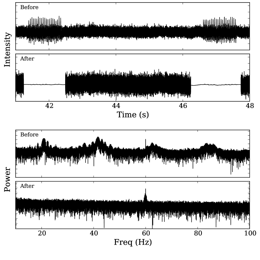
Figure 4.— An example of the effect of the bursts of interference caused by some of the electronics equipment at the Arecibo Observatory on PALFA survey data in time and frequency domain (labeled “Before”) and the same interval of time series and power spectrum after our finely-tuned removal algorithm, described in § 3.4.1, is applied (labeled “After”). Part of the time series is sacrificed, but the broad features in the frequency domain are completely removed. The RFI peak at 60 Hz that remains in the bottom panel is caused by the electrical mains and is later removed by zapping intervals of the power spectrum (described in § 3.4.5). The source of this interference signal has been identified and can be dealt with by shutting it off during PALFA observations.

3.4.2 Narrow-Band Masking

Every observation is examined for narrow-band RFI signals using PRESTO’s rfifind, which considers 2-s long blocks of data in each frequency channel separately. For each block of data two time-domain statistics are computed: the mean of the block data value, and the standard deviation of the block data values. Also, one Fourier-domain statistic is computed for each block: the maximum value in the power spectrum. Blocks where the value of one or more of these three statistics is sufficiently far from the mean of its respective distribution are flagged as containing RFI. For the two time-domain metrics, in the PALFA survey the threshold for flagging a block is 10 standard deviations from the mean of the distribution, and for the Fourier-domain metric, the threshold is 4 standard deviations from the mean. The resulting list of flagged blocks is used to mask out RFI. Masked blocks are filled with constant data values chosen to match the median bandpass. Channels that are more than 30 % masked are completely replaced, as are sub-integrations that are at least 70 % masked.

On average, only $\sim$ 5.75 % of time-frequency space is masked by this algorithm, and $\sim$ 93 % of observations have mask-fractions less than 10 %. Observations where the mask-fraction is larger than 15 % will be re-inserted into the list of sky positions to observe. These represent only $\sim$ 1.1 % of observations.

The fraction of data masked for each beam, and a graphical representation of the mask are stored in the results database as diagnostics of the observation quality.

Generating the rfifind mask makes up only $\sim$ 1 % of the total pipeline running time.

3.4.3 Time-Domain Clipping and Filtering

It is possible for broad-band impulsive interference signals to be missed by the masking procedure described above if the signals are not sufficiently strong to be detected in individual channels. Fortunately, the PALFA pipeline makes use of a complementary algorithm designed to remove such signals from the data: a list of bad time intervals is determined by identifying samples in the DM=0 $\mathrm{pc\,cm^{-3}}$ time series that are significantly larger ($>6\,\sigma_{\mathrm{loc}}$) than the surrounding data samples. The spectra corresponding to the bad time intervals are replaced by the local median bandpass.

As previously mentioned, for single-pulse searching, the PALFA pipeline also applies the PRESTO-implementation of the zero-DM filtering technique described in Eatough et al. (2009). This implementation enhances the original prescription by using the bandpass shape as weights when removing the DM=0 $\mathrm{pc\,cm^{-3}}$ signal. The zero-DM filter greatly reduces the impact of RFI on single-pulse searching, facilitating low-DM RRATs being distinguished from RFI. To illustrate the benefits of zero-DM filtering, Figure 5 shows a comparison of the single-pulse events identified by single_pulse_search.py in an observation of PSR J1908+0734 with and without filtering.

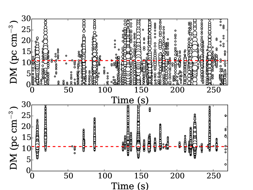
Figure 5.— Comparison of single-pulse events detected in a PALFA observation of PSR J1908+0734 in a search of the un-filtered time series (top) and the zero-DM filtered time series (bottom). Each circle represents the time and DM of an impulsive signal found by PRESTO’s single_pulse_search.py. The size of the circle is proportional to the significance of the signal (up to a maximum radius). Most of the RFI is filtered out of the observation by the zero-DM algorithm while leaving the pulsar pulses, albeit with some loss of significance at the lower DMs. Thus, the zero-DM filtering technique makes it far easier to disentangle astrophysical signal at non-zero DMs from RFI at DM=0 $\mathrm{pc\,cm^{-3}}$ both by eye and algorithmically. The pulsar’s DM=11 $\mathrm{pc\,cm^{-3}}$ is indicated with the dashed red line.

3.4.4 Red-Noise Suppression

In order to properly normalize the power spectrum and compute more correct false-alarm probabilities (see Ransom et al., 2002), we use a power spectrum whitening technique to suppress frequency-dependent, and in particular “red” noise. The median power level is measured in blocks of Fourier frequency bins and then multiplied by $\log 2$ to convert the median level to an equivalent mean level assuming that the powers are distributed exponentially (i.e. $\chi^{2}$ with 2 degrees-of-freedom).

The number of Fourier frequency bins per block is determined by the log of the starting Fourier frequency bin, beginning with 6 bins and increasing to approximately 40 bins by a frequency of 6 Hz. Above that frequency, where there is little to no “colored” noise, block sizes of 100 bins are used. The resulting filtered power spectrum has unit mean and variance. This process is accomplished with PRESTO’s rednoise program.

3.4.5 Fourier-Domain Zapping

Sufficiently bright periodic sources of RFI can be mistakenly identified as pulsar candidates by our FFT search. To excise, or zap, these signals from our data we tabulate frequency ranges often contaminated by RFI. The Fourier bins contained in this zap list are replaced by the average of nearby bins prior to searching.

The RFI environment at Arecibo is variable. The number, location, and width of interference peaks in the Fourier transform of DM=0 $\mathrm{pc\,cm^{-3}}$ time series vary on a time scale of months to years. To demonstrate this, the fraction of Fourier bins occupied by RFI as a function of epoch is illustrated in Figure 6. The median fraction of the Fourier spectrum occupied by RFI for all Mock spectrometer data for various intervals is: 2.9 % (0-10 Hz), 5.1 % (10-100 Hz), and 0.5 % (100-1000 Hz). To account for this dynamic nature of the RFI, we compute zap lists for each MJD.

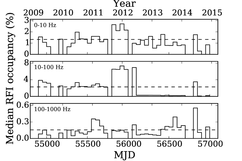
Figure 6.— Median percentage of the Fourier domain occupied by RFI in three frequency ranges for 50-day intervals (solid lines) compared against the median percentage for all observations (dashed lines). Many periodic sources of RFI are found to vary on daily time scales. Thus, lists of RFI-contaminated Fourier frequencies to be removed from the power spectrum prior to searching are tailored to the RFI of each MJD. The increase in RFI in the middle panel between MJD 55750 and 56100 was due to on-site electronics at the telescope, which since being identified in 2012 June (MJD $\simeq 56100$) has nearly always been turned off during PALFA observations, significantly reducing the RFI in the 10-100 Hz interval.

To compute zap lists we exploit the fact that RFI signals are typically detected by multiple feeds in a single 5-min pointing, or persist for most of an observing session (typically 1–3 hours). The strategy we employ here is similar to what was used in the Parkes Multibeam Pulsar Survey (Manchester et al., 2001). Fourier bins contaminated by RFI are determined by finding peaks in a median power spectrum, which is comprised of the bin-wise median of multiple DM=0 $\mathrm{pc\,cm^{-3}}$ power spectra. This is done twice, using two different subsets of data: a) all observations made with a given ALFA feed on a given day (to identify RFI signals that persist for multiple hours, or issues specific to the ALFA receiver), and b) all seven observations from a given pointing (to identify shorter-duration periodic RFI signals that enter multiple feeds). The zap list for any given observation is the union of the lists for its pointing and its feed.

With the advent of sophisticated candidate ranking and candidate classifying machine-learning algorithms (see § 3.5), it is better to leave some RFI in the data than to remove large swaths of the Fourier domain. To avoid excessive zapping we remove at most 3 % from each frequency decade, up to a maximum of 1 % globally, preferentially zapping bins containing the brightest RFI.

In addition to being an essential part of the PALFA RFI-mitigation strategy, zap lists have also proven to be a useful diagnostic for monitoring the RFI environment at Arecibo.

3.5. Post-processing Components

3.5.1 Ratings

A series of 19 heuristic ratings are computed for each folded periodicity candidate produced by the data analysis pipeline. These ratings encapsulate information about the shape of the profile, the persistence and broadbandedness of the signal, whether the frequency of the signal is particularly RFI-prone, and whether the signal is stronger at DM=0 $\mathrm{pc\,cm^{-3}}$. Each of the ratings is uploaded to the results database, and is available for querying and sorting candidates (see § 3.6). The ratings and brief descriptions are presented in Table 4.

The ratings are incorporated into candidate-selection queries along with standard parameters such as period, DM, and various measures of time-domain and frequency-domain significance. Using ratings in this way allows users to constrain the candidates they view to have certain features they would require when selecting promising candidates by eye. Alternatively, the ratings have been used in a decision-tree-based artificial intelligence (AI) algorithm, but this has since been supplanted by the more sophisticated “PICS” algorithm described in § 3.5.2 (Zhu et al., 2014).

The code to compute the ratings is compatible with the binary files produced by PRESTO’s prepfold for each periodicity candidate. For each candidate a text file is written containing the name, version, description, and value for all ratings being computed. This task is performed as part of the data analysis pipeline. The rating information is later uploaded to the results database. In cases where a new rating is devised, or an existing rating is improved, the prepfold binary files are fetched from the results archive, ratings are computed in a stand-alone process (i.e. independent of the pipeline), and the values are inserted into the database. The values of improved ratings are inserted alongside values from old versions to permit detailed comparisons.

3.5.2 Machine Learning Candidate Selection

All periodicity candidates are also assessed by the Pulsar Image-based Classification System (PICS; Zhu et al., 2014), an image-pattern-recognition-based machine-learning system for selecting pulsar-like candidates. The PICS deep neural network enables it to recognize and learn patterns directly from 2-D diagnostic images produced for every periodicity pulsar candidate. The large variety of pulsar candidates used to train PICS has developed its ability to recognize both pulsars and their harmonics.

PICS can reduce the number of candidates to be inspected by human experts by a factor of $\sim$ 100 while still identifying 100 % of pulsars and 94 % of harmonics to the top 1 % of all candidates (Zhu et al., 2014).

Since late 2013, PICS has been integrated directly into the PALFA processing pipeline. It produces a single rating for each candidate, which is uploaded into the results database as a rating (see § 3.5.1). So far, this has aided in the discovery of 9 pulsars (see § 4).

3.5.3 Coincidence Matching

While PALFA has been successful at finding moderately bright MSPs, the vast quantity of periodicity candidates close to the detection threshold at very short periods ($\stackrel{{\scriptstyle<}}{{{}_{\sim}}}$ 2 ms) have made it more challenging to identify the faint MSPs in the PALFA results database. To facilitate the process, a search for signals with compatible periods, DMs and sky positions has been performed on the periodicity candidates in the database. By applying our coincidence matching algorithm to the complete list of folded candidates we are able to reliably probe lower $S/N$s than would be reasonable to do thoroughly by manual viewing. This algorithm is complementary to our machine learning technique that operates on each candidate individually. The software developed to find matching candidates is available on the web for general use.

Large parts of the survey region have either been observed more than once or have been densely sampled (see Fig. 1), making it possible to match the detection of a pulsar from multiple observations confidently. For each observation, a list of beams from other pointings that fall within $5^{\prime}$ is generated. Candidates from the different beams are matched by their DMs and barycentric periods. Allowances are made for slightly different DMs and periods, as well as for harmonically related periods. Multiple matches that include the same candidate are consolidated to form groups of more than two candidates.

The results of this matching algorithm are examined with a dedicated, web-based interface. Many known pulsars, especially high harmonics of very bright slow pulsars, have already been identified.

As of 2015 January, our coincidence matching search has not yet resulted in the discovery of new pulsars, but it continues to be applied to the results database. This algorithm will be increasingly useful as more of the PALFA survey region becomes densely sampled, and as more Mock spectrometer observations cover positions previously observed with the WAPP spectrometers.

3.6. Collaborative Tools

The PALFA Consortium has created and made use of several online collaborative tools on the CyberSKA portal (Kiddle et al., 2011), a website developed to help astronomers build tools and strategies for large-scale projects in the lead-up to the Square Kilometre Array (SKA).

The CyberSKA portal allows for third-party applications to be accessed directly without a need for separate user authentication. Within this framework several PALFA-specific applications were developed:

Candidate Viewer – The primary method for viewing and classifying PALFA candidates is by using the CyberSKA Candidate Viewer application. It allows users to access the Cornell-hosted results database using form-based, free-text, and saved queries. Queries include basic observation and candidate information (e.g. sky position, period, DM, significance), as well as ratings (§ 3.5.1), and the PICS classifications (§ 3.5.2). Users are presented with a series of prepfold diagnostic plots in sequence, one for each candidate matching the query. By inspecting the plots, as well as other relevant information provided, such as a histogram showing the number of occurrences of signals in the relevant frequency range as well as a summary plot showing all the beam’s periodic signal candidates in a period-DM plot, the user can quickly classify candidates. Classifications are saved to the database and can be easily retrieved.

Top Candidates – Especially promising candidates found with the Candidate Viewer can be added to the Top Candidates application, which is designed to store the most likely pulsar candidates. The application also allows collaboration members to view and vote on which candidates should be subject to confirmation observations, as well as help organize and track these observations and their outcomes.

Survey Diagnostics – Optimizing the use of telescope time and computing resources is extremely important for large-scale pulsar surveys such as PALFA. The Survey Diagnostics application automatically compiles a set of information and a set of plots from various sources to help the project run smoothly. This includes the status of data acquisition and reduction, the severity of the RFI environment, and the quality of the data.

4. Results

The PALFA Survey has discovered 145 pulsars, including 19 MSPs and 11 RRATs, and one FRB, as of 2015 March. The PRESTO-based pipeline described in § 3 has discovered 41 pulsars from their periodic emission, 5 RRATs from their impulsive emission, and re-detected another 60 pulsars that were previously discovered with other PALFA data analysis pipelines. The other pulsars found in the PALFA survey were discovered with the different data analysis pipelines, such as the E@H and Quicklook pipelines (Allen et al., 2013; Stovall, 2013) which use complementary RFI-excision and search algorithms, with dedicated transient searches, or in earlier observations with the WAPP spectrometers using an earlier version of the pipeline described here. Not all sky positions observed with the WAPP spectrometers have been covered with the Mock spectrometers yet.

We report details for 41 of the periodicity-discovered pulsars found in Mock spectrometer data with the pipeline described above. All but one of these discoveries are in the inner Galaxy region. These pulsars were discovered by analyzing 85333 beams, covering a total of 134 sq. deg., which consists of 80 sq. deg. in the inner Galaxy region, and 54 sq. deg. in the outer Galaxy region (see Table 2). Basic parameters of the discoveries are in Table 5, and pulse profiles from the discovery observations are shown in Figure 7.

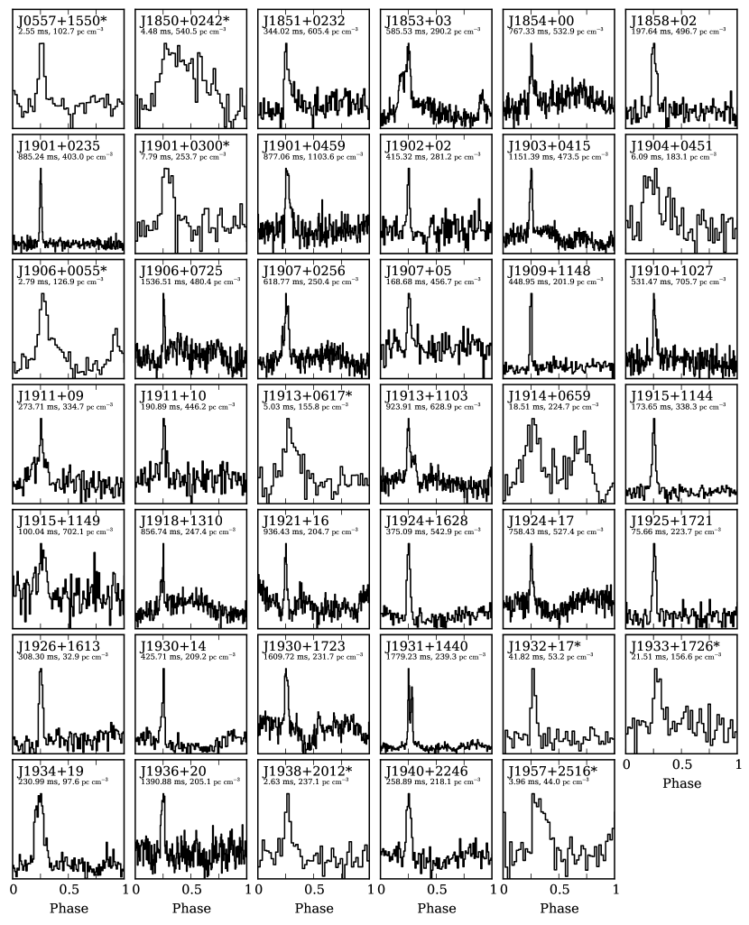
Figure 7.— Pulse profiles at 1.4 GHz from the discovery observations of the 41 pulsars discovered with the PRESTO-based PALFA pipeline in Mock spectrometer data. The name of each pulsar is included above each profile along with the period, and dispersion measure. The names of binary pulsars are indicated with an asterisk (*). The number of bins across the profile is what was used by the pipeline, and is larger for longer period pulsars. These profiles also include intra-channel DM smearing, which is most significant for high-DM, short-period pulsars. The baselines of several profiles, predominantly of the long-period pulsars, show broad features due to interference and red noise in the data (for example, PSRs J1854+00, J1921+16, and J1930+1723). The discovery profiles contaminated with RFI and red noise are shown here to highlight the ability of the PALFA pipeline to identify pulsars despite these conditions. Pulsars with truncated names do not yet have positions determined from timing campaigns.

Eight of the 41 pulsars reported here are MSPs, including the most distant MSP (based on its DM) discovered to date, PSR J1850+0242. The distance estimated from the DM of PSR J1850+0242, assuming the NE2001 model (Cordes & Lazio, 2002), is 10.4 kpc, a testament to the ability of the PALFA survey to find highly dispersed, short period pulsars. PSR J1850+0242, along with three of the other MSPs discoveries reported here are described in detail in Scholz et al. (2015). Three more of the MSPs reported here will be included in Stovall et al. (in prep.).

Nine of the 41 pulsars reported here are in binary systems, including seven of the MSPs, and two slower pulsars, PSRs J1932+17 ($P\simeq 42$ ms) and J1933+1726 ($P\simeq 22$ ms), that were spun-up by the accretion of mass and transfer of angular momentum, the so-called “recycling” process (Alpar et al., 1982). The timing analysis of PSR J1933+1726 will be provided by Stovall et al. (in prep.)

Timing solutions for six of the slow pulsars presented in this work, including the young PSR J1925+1721, will be published in a forthcoming paper along with the timing of other PALFA-discovered pulsars (Lyne et al., in prep.).

In addition to the 41 periodicity pulsars detailed here, the PRESTO-based pipeline has found 5 RRATs. The beams containing these RRATs were identified using a post-processing algorithm originally developed for pulsar surveys at 350 MHz with the Green Bank Telescope (see Karako-Argaman et al., 2015, for details). Discovery parameters and detailed follow-up observations for these RRATs will be described elsewhere.

4.1. Estimating Flux Densities of New Discoveries

The flux densities of the new discoveries were estimated using the radiometer equation (Dewey et al., 1985),

$$S_{\mathrm{est}}=\frac{\left(S/N\right)_{T}\left(T_{\mathrm{sys}}+T_{\mathrm{sky}}\right)}{G(\theta,ZA)\sqrt{n_{p}t_{\mathrm{obs}}\Delta f}}\sqrt{\frac{W}{P-W}},$$ (3)

where relevant parameters are the pulse profile width, $W$, the telescope gain, $G(\theta,ZA)$, the number of polarization channels summed, $n_{p}$, the observation length, $t_{\mathrm{obs}}$, the observing bandwidth, $\Delta f$, the period of the pulsar, $P$, the system and sky temperatures, $T_{\mathrm{sys}}$ and $T_{\mathrm{sky}}$, respectively. The time-domain signal-to-noise ratio, $\left(S/N\right)_{T}$, was measured from folded profiles using the area under the pulse and the off-pulse RMS.

In some cases, predominantly for long-period pulsars, the baseline of the pulse profile exhibited broad features, likely due to red noise. (See some examples in Fig. 7.) To more robustly estimate flux densities, we fit Gaussian components to the pulse profile, including the broad off-pulse features. The integrated pulsar signal was determined from the on-pulse components, and the noise level of the profile was determined from the standard deviation of the residuals after subtracting all fitted components from the profile.

The gain was scaled according to the angular offset of the pulsar from the beam center, $\theta$, assuming an Airy disk beam pattern with $\mathrm{FWHM}=3\farcm 35$ (Cordes et al., 2006), as well as the dependence on the zenith angle, $ZA$. The gain also took into account the ALFA beam with which the pulsar was detected, $G(0)=10.4$ K/Jy for the central beam, and $G(0)=8.2$ K/Jy for the outer 6 beams (Cordes et al., 2006).

Sky temperatures were scaled from the Haslam et al. (1982) 408-MHz survey to 1400 MHz using a spectral index of $-2.76$ for the Galactic synchrotron emission (Platania et al., 1998). The sky temperatures also include the 2.73 K cosmic microwave background.

The resulting phase-averaged flux density estimates of the PALFA pulsars discovered with our pipeline range from 16 $\mu$Jy to 280 $\mu$Jy (see Table 5), making them among the weakest detected pulsars in the Galactic field, along with other PALFA-discovered pulsars (see Fig. 8).

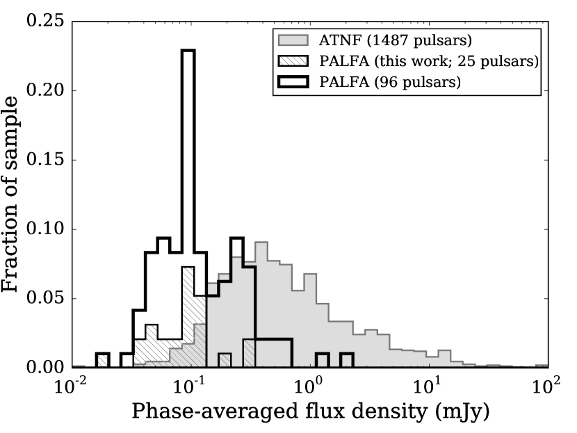
Figure 8.— Distribution of phase-averaged flux densities of pulsars discovered in the PALFA survey, and the distribution of 1400-MHz phase-averaged flux densities from the ATNF pulsar catalogue of all non-PALFA, non-globular cluster discoveries. The sub-set of PALFA pulsars featured in this work is highlighted. Only PALFA-discovered pulsars with timing positions are included.

4.2. Re-Detections of Known Pulsars

In total, 83 pulsars for which 1400-MHz phase-averaged flux densities, $S_{1400}$, are reported in the ATNF catalogue were detected with the Mock spectrometers in 268 different PALFA observations (i.e. some known pulsars were re-detected multiple times).

To confirm that our observing set-up is as sensitive as expected, we estimate the $\left(S/N\right)_{T}$ at which our pipeline should blindly re-detect known pulsars in our observations and compare with the $\left(S/N\right)_{T}$ measured from the profile of the corresponding candidate. The expected $\left(S/N\right)_{T}$ values were estimated by inverting Eq. 3 to solve for the signal-to-noise ratio using $S_{1400}$ from the ATNF catalogue. As in § 4.1 the telescope gain is modeled as an Airy disk with $\mathrm{FWHM}=3\farcm 35$.

By comparing expected and measured signal-to-noise ratios against pulsar spin period we find that longer-period pulsars show an increase scatter in $\left(S/N\right)_{T}$ ratio as well as a bias towards larger ratios (see Fig. 9). This is consistent with the reduced sensitivity to long-period pulsars due to red noise we find from our sensitivity analysis using synthetic pulsar signals (see § 5).

In addition to the 83 known pulsars with published $S_{1400}$ detected with the PALFA PRESTO pipeline, there are 50 more that do not have values for $S_{1400}$ listed in the ATNF catalogue. The complete list of 128 previously discovered pulsars blindly re-detected by the PALFA PRESTO pipeline is in Table LABEL:tab:redetections.

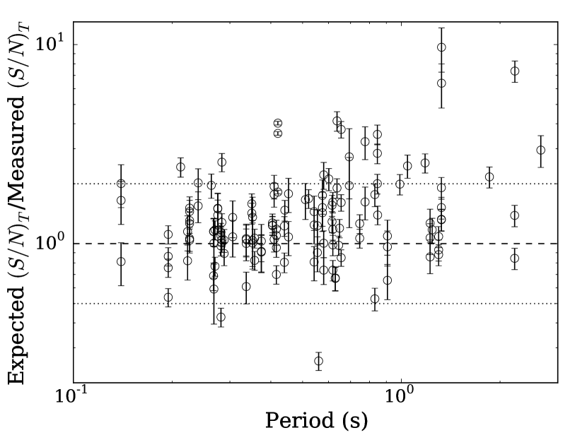
Figure 9.— Ratio of expected and measured $\left(S/N\right)_{T}$ as a function of pulsar period. Expected $\left(S/N\right)_{T}$ values are calculated using the radiometer equation and measured flux densities at 1400 MHz from the ATNF catalogue. Measured $\left(S/N\right)_{T}$ values are computed from detections of known pulsars in PALFA observations. The increased scatter and bias towards higher $S/N$ ratios of longer-period pulsars are consistent with reduced sensitivity to these pulses due to red noise (see § 5.4 and Fig. 11). Known pulsars without reported flux densities and uncertainties are excluded, as are pulsars that have reported flux densities consistent with 0 mJy. Also excluded from the plot are 15 known pulsars with published flux densities that were detected in observations pointed more than $3^{\prime}$ from the position of the pulsar. This is because the actual beam pattern differs considerably from the theoretical Airy disk beam pattern beyond $\sim$ $3^{\prime}$, making it difficult to reliably estimate the expected $\left(S/N\right)_{T}$. The dashed line indicates equality of the expected and measured $\left(S/N\right)_{T}$ values, and the dotted lines are at a factor of two above and below equality.

4.3. Known Pulsars Missed

In addition to the 268 detections of 128 separate known pulsars mentioned in § 4.2, there were 7 instances in which a known pulsar was not detected by the search pipeline, despite being detected when subsequently folding the search data with the most recently published ephemeris. In all cases the data were badly affected by RFI; there are strong signals within one Fourier bin of the pulsar period. Furthermore, these are long-period pulsars, which are more difficult to detect than expected due to red noise in the data. It is therefore not entirely surprising that these observations did not result in detections. A thorough analysis of the effects of RFI and red noise on the sensitivity to long period pulsars is therefore crucial, and forms the discussion of the following section.

5. Assessing the Survey Sensitivity

The sensitivity of pulsar observations is typically estimated using the radiometer equation (Eq. 3). In principle, the effects of DM, period, and pulse width on sensitivity are adequately described by the radiometer equation. The expression derived by Cordes & Chernoff (1997, see their Appendix A), includes a more complete description of pulse shape and the effect of DM, which causes distortions of the pulse profile. However, neither of these equations includes the effect of RFI. In this section, we describe a prescription for accurately modeling the sensitivity of pulsar search observations including the effect of RFI, as well as its dependence on period, DM, and pulse width.

To estimate the survey sensitivity we injected synthetic pulsar signals into actual survey data, and attempted to recover the period and DM of the input signal using our pipeline. By using synthetic signals we can also better determine the selection effects imposed by our pipeline.

5.1. Constructing a Synthetic Pulsar Signal

For this work, a simple synthetic pulsar signal was constructed for a given combination of period, DM, phase-averaged flux density, and profile shape. Once the relevant parameters were chosen (see § 5.3 and Table 7), a two-dimensional pulse profile (intensity vs. spin phase and observing frequency) was generated.

The pulse profile of each frequency channel was smeared by convolving with a box-car whose phase width corresponded to the dispersion delay within the channel, as well as scattered by convolving with a one-sided exponential function with a characteristic phase width corresponding to the pulse broadening time scale. We determined the scattering time scale using Eq. 1. Care was taken to conserve the area under the profile during the convolutions. The scaling factor applied to the synthetic signals was determined by flux-calibrating the PALFA observing system (see §5.2).

5.2. Calibration

On 2013 December 21, we observed the radio galaxy 3C 138 in order to calibrate the central beam of ALFA. Three observations using the standard survey set-up described in §2 were conducted, but with 5-min integrations, and with the calibration diode being pulsed on and off at 40 Hz. The on-source scan of 3C 138 was preceded by an off-source scan 0.5^∘ to the north of 3C 138 and followed by a similar off-source scan 0.5^∘ to the south.

The calibration observation data were converted to 4-bit samples, and the Mock spectrometer sub-bands were combined (see § 3.2). The data were folded at the modulation frequency of the calibrator diode using fold_psrfits of psrfits_utils. Next, the on-cal and off-cal levels in the on-source and off-source observations were used to relate the flux density of the calibration diode with the cataloged flux density of 3C 138 (for details, see e.g. Lorimer & Kramer, 2004). The result is the flux density of the calibration diode as a function of observing frequency. In practice, this was done using fluxcal of psrchive .

The per-channel scaling factors between flux density and the observation data units were determined by applying the calibration solution along with the calibration diode signal. This procedure determines the absolute level of the injected signal corresponding to a target phase-averaged flux density, as well as the shape of the bandpass.

5.3. Injection Trials

Artificial pulsar signals were injected into the data by summing the two-dimensional, smeared, scattered, and scaled synthetic pulse profile with the data at regular intervals corresponding to the period of the synthetic pulsar. The scaling was determined using the calibration procedure described in § 5.2. The resulting data file, including the injected signal, was written out with 32-bit floating-point samples in SIGPROC “filterbank” format to avoid having to quantize the weak synthetic pulsar signal.

Many synthetic signals with a broad range of parameters were required to build a comprehensive picture of the survey sensitivity (see Table 7). In total, 17 periods were selected between 0.77 ms and 11 s along with six DMs ranging from 10 to 600 $\mathrm{pc\,cm^{-3}}$. In all cases, the profile of the synthetic signal was chosen to have a single centered von Mises component with a FWHM selected from 5 possible values between $\sim$1.5 % and $\sim$24 % of the period. The example profile in Figure 10 shows the case where FWHM=2.6 %. The synthetic signals were injected into 12 different observations to determine the survey sensitivity in a variety of RFI conditions. All 12 observations used in this analysis are from late 2013 and from the central beam of ALFA. Although the gains of the outer beams are lower than that of the central beam, the response of the observing system and pulsar search pipeline to RFI and red noise derived for the central beam should also apply to the outer beams.

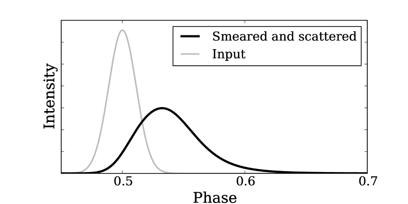
Figure 10.— The profile of a synthetic $P=5$ ms pulsar consisting of a single von Mises component with FWHM=2.6% (gray), and the same profile broadened according to DM=250 $\mathrm{pc\,cm^{-3}}$. The broadening is caused by dispersive smearing within each channel and scattering according to Eq. 1. Note that the plot is zoomed into the region: $0.45<\phi<0.7$.

The total number of combinations of synthetic signals and observations is $>$ 6000. Multiple trials, each with a different amplitude, were constructed, injected, and searched to determine the sensitivity limit at each point in (period, DM, pulse FWHM) phase-space. To reduce the computational burden, not all possible combinations of parameters were used. In particular, only the profile with FWHM $\sim$3 % was injected into all 12 observations. The remaining four profiles shapes were only injected into a single observation. This still permits the determination of the dependence of $S_{\mathrm{min}}$ on pulse width.

5.4. Realistic Survey Sensitivity

It is well known (Dewey et al., 1985) that the minimum detectable flux density of a pulsar depends on the intrinsic width of its profile, as well as the DM, because dispersive smearing and scattering broaden the profile. It is also reasonable to expect a reduction of sensitivity due to RFI and red noise, even with the red noise suppression algorithms employed (see § 3.4.4). By recovering injected signals using the pipeline described in § 3, we have determined the true sensitivity of the PALFA survey, and its dependence on spin period and DM (see Fig. 11). We found the commonly used version of the radiometer equation (Eq. 3; Dewey et al., 1985) overestimates the survey sensitivity to long-period pulsars. For example, for $P=0.1$–2.0 s pulsars with DM $>150$ $\mathrm{pc\,cm^{-3}}$ (the majority of the pulsars we expect to find with PALFA), the degradation in sensitivity compared with the ideal case is a factor of $\sim$1.1–2.

We have also confirmed the claim by Cordes & Chernoff (1997) that the Dewey et al. (1985) radiometer equation underestimates the sensitivity to high-DM MSPs, by not correctly modeling the distortion of the profile due to smearing and scattering. The more accurate variant of the radiometer equation from Cordes & Chernoff (1997) better matches our measured sensitivity curves in the MSP regime, thanks to its inclusion of the profile shape and distortions. However, the degraded sensitivity we find at long periods is still not properly modeled with these adjustments.

Red noise present in pulsar search data due to RFI, receiver gain fluctuations, and opacity variations of the atmosphere makes it difficult to detect long-period radio pulsars. Our analysis has shown that for the PALFA survey, at low DMs, the reduction in sensitivity already affects pulsars with periods of $\sim\!100$ ms. Fortunately, the effect is slightly less significant for pulsars with higher DMs. This is evident in Figure 11.

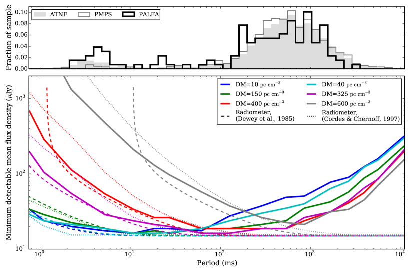
Figure 11.— Top – Period distribution of all Galactic radio pulsars, excluding RRATs, listed in the ATNF catalogue, as well as those found in the PALFA and Parkes Multibeam Pulsar Survey (PMPS).
Bottom – Minimum detectable phase-averaged flux density curves for the PALFA survey as determined using synthetic pulsar signals with FWHM=2.6 %. The reduction in sensitivity at long periods is due to red noise in the data. We see clear discrepancies when comparing the measured curves with the analogous sensitivity limits derived with the commonly used radiometer equation (Dewey et al., 1985). Sensitivity to long-period pulsars is overestimated, and sensitivity to MSPs is underestimated. However, the formulation of the radiometer equation by Cordes & Chernoff (1997) is more complete – albeit less frequently used – and better models the sensitivity in the short-period regime. See § 5.4.

We have parameterized the sensitivity curves by fitting $\log S_{\mathrm{min}}$ vs. DM with a quadratic function and modeling how these curves depend on period. To estimate $S_{\mathrm{min}}$ at an arbitrary profile width, we first estimate $S_{\mathrm{min}}$ at each of the five trial widths, then fit a quadratic function in $\log S_{\mathrm{min}}$ vs. width, and use the parameters of the fit to calculate $S_{\mathrm{min}}$ at the desired width. This ad-hoc scheme provides reliable estimates of $S_{\mathrm{min}}$ within the intervals used for trial values of period, DM, and width, as well as for modest extrapolation. Sensitivity maps for each of the five profile widths used are shown in Figure 12.

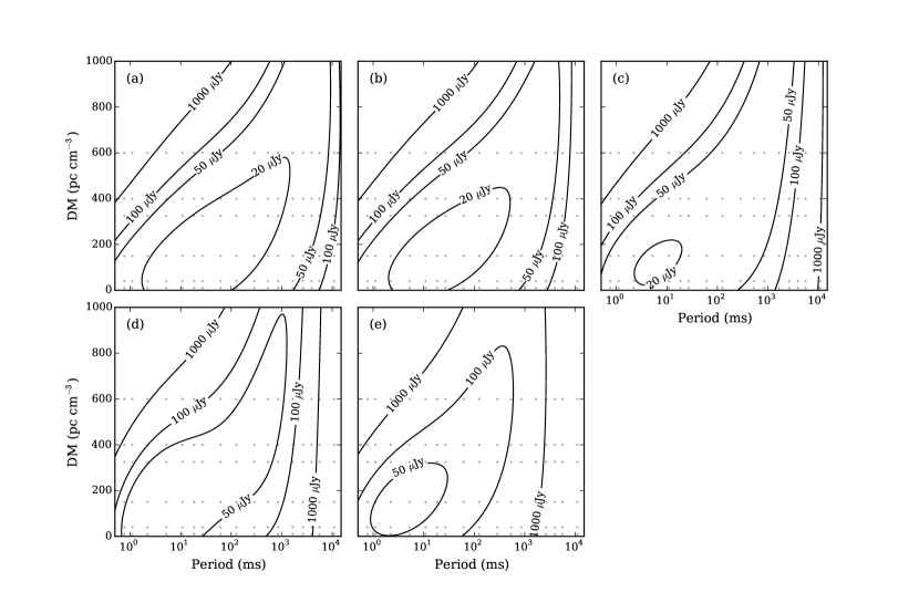
Figure 12.— PALFA survey sensitivity as a function of DM and spin period. The maps are determined using synthetic pulsar signals injected into observations and recovered using the pipeline. Contours correspond to minimum detectable phase-averaged flux densities of 20, 50, 100, 1000 $\mu$Jy. The five panels (a)–(e) correspond to profile FWHMs of 1.5, 2.6, 5.9, 11.9, 24.3 %, respectively. In all cases, the profile consists of a single centered von Mises component (see Fig. 10 for an example). The period, DM combinations used in the sensitivity analysis are shown with the small dots.

6. Population Synthesis Analysis

We have used the sensitivity curves determined above (see § 5.4) to re-evaluate the expected yield of the PALFA survey by performing a population synthesis analysis with PsrPopPy (Bates et al., 2014).

Galactic populations of non-recycled pulsars were simulated using the radial distribution from Lorimer et al. (2006b) and a Gaussian distribution of heights above/below the plane with a scale height of 330 pc. The pulsar periods were described by a log-normal distribution with $\left<\log P\right>=2.7$ and $\sigma_{\log P}=-0.34$ (Lorimer et al., 2006b). The pulse-width-to-period relationship was also taken from Lorimer et al. (2006b). We used a log-normal luminosity distribution described by the best-fit parameters found by Faucher-Giguère & Kaspi (2006), $\left<\log L\right>=-1.1$ and $\sigma_{\log L}=0.9$.

We created 5000 simulated pulsar populations, each containing enough pulsars such that a simulated version of the Parkes multi-beam surveys detected 1038 pulsars, the number of non-recycled pulsars detected by the actual surveys. We then compared the pulsars in each of these populations against a list of PALFA observations, and estimated their significance using the radiometer equation. Pulsars with $(S/N)_{\mathrm{expect}}>11.3$ were considered detected. Next, we compared the flux-density for each “detected” pulsar against the parameterized PALFA sensitivity curves to determine if the pulsar also has a sufficiently large flux density to lie above the measured sensitivity curves. For each pulsar, the measured sensitivity curves are shifted according to the zenith angle of the observation, the gain of the beam used, the sky temperature and the angular offset between the pulsar position and the beam center.

We found $35\pm 3$ % of the simulated pulsars having fluxes above the theoretical sensitivity threshold derived from the radiometer equation (Eq. 3) are not sufficiently bright to be “detected” by our measured sensitivity limits for the PALFA survey (e.g. Fig. 12) due to the residual effect of red noise and RFI following the extensive mitigation procedures described in § 3.4. The median period of the pulsars missed is $P_{\mathrm{miss}}\simeq 566$ ms, which is considerably longer than the median period of the potentially detectable pulsars brighter than the radiometer-equation-based threshold, $P_{\mathrm{det.}}\simeq 440$ ms (see Fig. 13).

Our 5000 realizations of simulated Galactic pulsar populations, adjusted for the reduced sensitivity to long-period pulsars, suggest $217\pm 15$ un-recycled pulsars should be detected in PALFA Mock spectrometer observations, given the current processed pointing list. As of 2015 January, 241 un-recycled pulsars have been discovered/detected in PALFA observations with the Mock spectrometers.

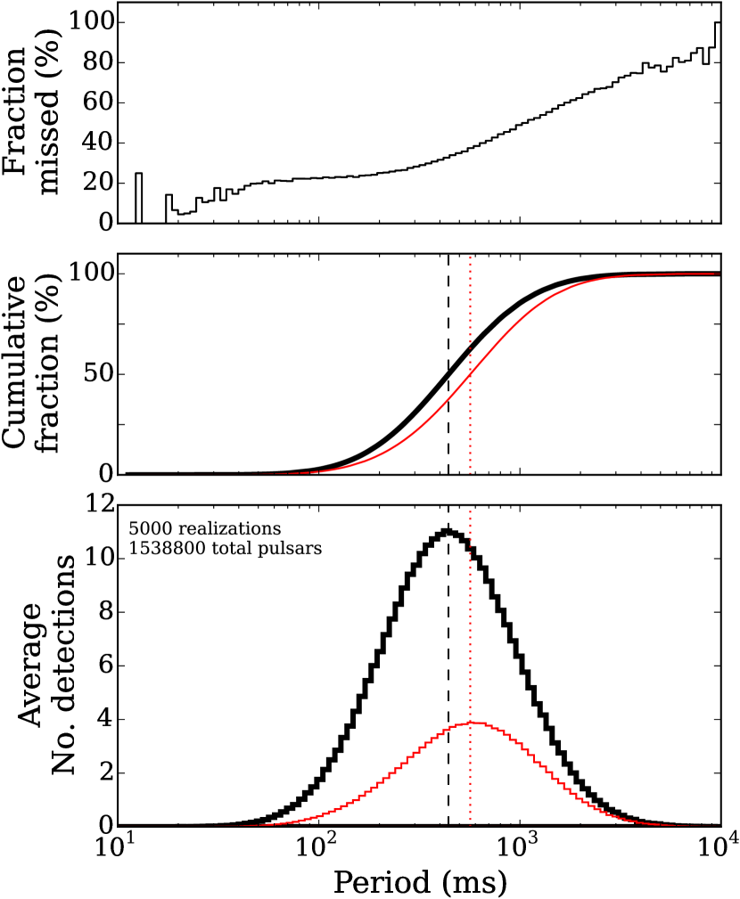
Figure 13.— Top – Fraction of potentially detectable pulsars missed by PALFA due to red noise as a function of spin period, assuming the underlying pulsar population is accurately modeled by our input distributions (i.e. the distributions in Lorimer et al. (2006b), see § 6).
Middle – Cumulative fraction of simulated pulsars (thick black line), and pulsars missed (thin red line) as a function of pulse period.
Bottom – Period distribution of potentially detectable simulated population of un-recycled pulsars averaged over 5000 realizations (thick black line) compared with the period distribution of pulsars expected to be missed due to red noise (thin red line). The median spin period of the potential detectable pulsars ($P\simeq 440$ ms) is shown by the dashed black line, and the median spin period ($P\simeq 566$ ms) of the missed pulsars is shown by the dotted red line.

The number of un-recycled pulsar detections predicted for the PALFA survey by Swiggum et al. (2014) is an overestimate for two reasons. First, their analysis used a threshold $S/N$ $=9$. Given the observing parameters assumed, a more appropriate threshold of $S/N$ $=11.3$ should have been used to correspond to the minimum detectable flux density we find ($S_{\mathrm{min}}=0.015$ mJy). Second, the analysis by Swiggum et al. (2014) did not include the effect of red noise, which we have shown reduces the number of pulsars expected to be found in the PALFA survey by 35%.

7. Discussion

The detailed sensitivity analysis of § 5.4 confirms that, on average, the PALFA survey is as sensitive to MSPs and mildly recycled pulsars as expected from the radiometer equation. However, the survey is less sensitive to long-period pulsars than predicted. The degradation in sensitivity is between 10% and a factor of 2 for the majority of pulsars we expect to find in the PALFA survey (spin periods between 0.1 s and 2 s and DM $>150$ $\mathrm{pc\,cm^{-3}}$), and up to a factor of $\sim 10$ in the worst case (DM $<100$ $\mathrm{pc\,cm^{-3}}$ and P $>2$ s; this fortunately corresponds to a parameter space that contains far fewer expected pulsars). The reduction of sensitivity is likely caused by red noise present in the observations.

The empirical sensitivity curves we determined apply specifically to the PALFA survey, its observing set-up, and the search algorithms used. Because the effects of red noise on radio pulsar survey sensitivity have the potential to be significant, as in the case of PALFA, we strongly suggest measuring the impact of red noise on other surveys by performing similar analyses to what we described in § 5. Also, future population analyses should include these measured effects of red noise rather than assuming the theoretical radiometer equation (e.g. Lorimer et al., 2006b; Faucher-Giguère & Kaspi, 2006) when deriving spatial, spin, and luminosity distributions for the underlying Galactic population of pulsars.

What are the potential ramifications of reduced sensitivity to long-period pulsars being unaccounted for in population synthesis analyses? First, the existence of radio-loud pulsars beyond the “death line” is important to our understanding of the radio emission mechanism in pulsars. For example, the existence of the 8.5-s PSR J2144$-$3933 contradicted several existing emission theories (Young et al., 1999; Zhang et al., 2000). The existence of a larger population of slowly rotating pulsars, particularly the discovery of pulsars so slow that existing theories cannot explain their radio emission, would further constrain models.

It is also possible there is a larger population of highly magnetized rotation-powered pulsars and quiescent radio-loud magnetars that have been missed by the lower than predicted sensitivity of pulsar surveys. Radio emission from three of the four known radio-loud magnetars was detected following high-energy radiative events (Camilo et al., 2006, 2007; Shannon & Johnston, 2013; Eatough et al., 2013). However, the other radio-loud magnetar PSR J1622$-$4950 was discovered from its radio emission (Levin et al., 2010; Olausen & Kaspi, 2014). There is no evidence that the turn-on of PSR J1622$-$4950 at radio wavelengths was preceded by a high-energy event. The possibility that radio emission from magnetars is not always accompanied by X-ray or $\gamma$-ray emission means it is crucial to understand the biases against finding such long-period pulsars. Characterizing, and hopefully uncovering a hidden population of radio-loud magnetars, as well as highly magnetized-rotation powered pulsars, will help clarify the relationship between these two classes of pulsars, as well as the influence of strong magnetic fields on emission properties (e.g flux and spectral index variability).

It may be possible to address the reduced sensitivity to long-period pulsars by utilizing algorithms that perform better in the presence of red noise, as well as algorithms that remove red noise without suppressing the pulsar signal.

Long-period pulsars may be found via their harmonics even if red noise obscures the signal in the Fourier domain at the fundamental frequency of the pulsar. The detection of the pulsar signal will be reduced in two ways. First, the harmonic summing algorithm will exclude the power contained at the fundamental and low harmonic frequencies, which can contain large amounts of power, especially in the case of pulsars with wide profiles. Second, by not being based at the fundamental frequency of the pulsar, the harmonic summing algorithm will skip slower, more significant harmonics in favor of weaker harmonics at higher frequencies. Despite the reduction in sensitivity several pulsars have been found in the PALFA survey thanks to their higher harmonic content.

One suggested method of improving sensitivity to long-period pulsars is by using the Fast-folding algorithm (FFA; see e.g. Lorimer & Kramer, 2004; Kondratiev et al., 2009, and references therein). The periodograms produced by the FFA, a time-domain algorithm, are generated from computing a significance metric from pulse profiles. Thus, the broad profile features caused by red noise pose a problem for FFA-based searches. In short, the FFA is not immune to the degradation of sensitivity to long-period pulsars described above. However it does have the advantage of coherently summing all harmonics of a given period and greater period resolution than the DFT. These two factors should make the FFA slightly more sensitive to long-period pulsars, especially those with narrow profiles, than the Fourier Transform techniques described in § 3.3.2, which is limited in the number of harmonics that can be summed (typically incoherently; Kondratiev et al., 2009). The FFA has only been used sparingly in large-scale pulsar searches (e.g. Kondratiev et al., 2009). A more systematic investigation and application of the FFA is warranted.

Another algorithm that might have better performance in the presence of red noise is the single-pulse search technique described in § 3.3.3. Single-pulse search algorithms are known to be more sensitive than standard FFT techniques to long-period pulsars in short observations (Deneva et al., 2009; Karako-Argaman et al., 2015). This is because of the natural variability of pulsar pulses and small number of pulses. Pulse-to-pulse variability was not included in the synthetic pulsar signals used in our sensitivity analysis and no single pulse searching was performed. It is likely that the sensitivity curves determined in this work are partially compensated by the single-pulse search techniques already in place, especially considering the recent suggestion that pulsars with $P>200$ ms have a greater likelihood of being detected in single-pulse searches than faster pulsars (Karako-Argaman et al., 2015). However, the extent of this compensation depends on the pulse-energy distributions of pulsars and the relative significances of their detections in periodicity and single-pulse searches.

8. Conclusions

We described the PRESTO-based PALFA pipeline, the primary data analysis pipeline used to search PALFA observations made with the Mock spectrometers. This pipeline has led to the discovery of 41 periodicity pulsars and 5 RRATs, the re-detection of 60 pulsars previously discovered in the survey (using other pipelines), and the detection of 128 previously known pulsars. The PRESTO-based pipeline described here consists of several complementary search algorithms and RFI-mitigation strategies. The performance of the pipeline was determined by injecting synthetic pulses into actual survey observations and recovering the signals.

We have found that the PALFA survey is as sensitive to fast-spinning pulsars as expected by the theoretical radiometer equation. However, in the case of long-period pulsars, we have found that there is a reduction in the sensitivity due to RFI and red noise in the observations. The actual detection threshold for pulsars with $P>4$ s at $\mathrm{DM}<150$ $\mathrm{pc\,cm^{-3}}$ is up to $\sim$ 10 times higher than predicted by the theoretical radiometer equation. We have performed a population synthesis analysis using this empirical model of the survey sensitivity. Our analysis indicates that $35\pm 3$ % of pulsars, with predominantly long periods, are missed by PALFA, compared to expectations based on theoretical sensitivity curves derived using the radiometer equation.

The magnitude of the effect of red noise on the PALFA survey’s sensitivity to long-period pulsars is surprising and should be taken into account in future population synthesis analyses. Furthermore, the effect of red noise on other radio pulsar surveys should be quantified in a similar manner and be included in population synthesis analyses to ensure the distributions determined for the underlying pulsar population are robust. The presence of more long-period pulsars could have implications on the location of the pulsar death line, the structure of pulsar magnetospheres and radio emission mechanism, as well as the relationship between canonical pulsars, highly magnetized rotation-powered pulsars, radio-loud magnetars, and RRATs.

Table 1PALFA Mock Spectrometer Observing Set-up Parameters

Parameter	Value
General
Sample Time, $\tau_{\mathrm{samp}}$ ($\mu$s)	65.476
Integration Timea, $t_{\mathrm{obs}}$ (s)	268 (Inner Galaxy, 32∘ $\stackrel{{\scriptstyle<}}{{{}_{\sim}}}$ $l$ $\stackrel{{\scriptstyle<}}{{{}_{\sim}}}$ 77∘)
	180 (Anti-Center, 168∘ $\stackrel{{\scriptstyle<}}{{{}_{\sim}}}$ $l$ $\stackrel{{\scriptstyle<}}{{{}_{\sim}}}$ 214∘)
High Sub-Band
Number of Channels	512
Low Frequency (MHz)	1364.290
High Frequency (MHz)	1536.016
Low Sub-Band
Number of Channels	512
Low Frequency (MHz)	1214.290
High Frequency (MHz)	1386.016
Merged Band
Number of Channels	960
Low Frequency (MHz)	1214.290
Center Frequency (MHz)	1375.489
High Frequency (MHz)	1536.688
Bandwidth, $\Delta f$ (MHz)	1322.398
Channel Bandwidth, $\Delta f_{\mathrm{chan}}$ (kHz)	1335.831

^aThis includes the $\sim 5-10$ s when the calibration diode is turned on, which is not usable for searching for pulsars. The interval of the observation containing this calibration signal is removed prior to our analysis (see § 3.2).

Table 2Breakdown of PALFA Mock Spectrometer Data

	No. Beamsa	No. Unique	Sky Coverage	Completenessb, $|b|<$2∘	Completenessb, $|b|<$5∘
		Sky Positions	(sq. deg.)	(%)	(%)
Inner Galaxy (32∘ $\stackrel{{\scriptstyle<}}{{{}_{\sim}}}$ $l$ $\stackrel{{\scriptstyle<}}{{{}_{\sim}}}$ 77∘)
Observed	40705	38479	94	69	32
Archived	35030	33243	81	60	27
Analyzed	33888	32499	80	58	27
Anti-Center (168∘ $\stackrel{{\scriptstyle<}}{{{}_{\sim}}}$ $l$ $\stackrel{{\scriptstyle<}}{{{}_{\sim}}}$ 214∘)
Observed	60305	26194	64	30	18
Archived	52659	21990	54	23	15
Analyzed	51445	21899	54	23	15

^aThere are 7 beams per pointing.
^bThe completeness percentages are relative to the number of pointings we will eventually cover with the Mock spectrometers.

Table 3Dedispersion Plan for Mock Spectrometer Data

DM range	DM step size	No. DMs	No. sub-bands	Sub-band DM spacing	Down-sample factor	Approx. Computing
($\mathrm{pc\,cm^{-3}}$)	($\mathrm{pc\,cm^{-3}}$)			($\mathrm{pc\,cm^{-3}}$)		(%)
$0-212.8$	0.1	2128	96	7.6	1	73.19
$212.8-443.2$	0.3	768	96	19.2	2	12.20
$443.2-534.4$	0.3	304	96	22.8	3	8.13
$534.4-876.4$	0.5	684	96	38.0	5	2.93
$876.4-990.4$	0.5	228	96	38.0	6	2.44
$990.4-1826.4$	1.0	836	96	76.0	10	0.73
$1826.4-3266.4$	2.0	720	96	144.0	15	0.24
$3266.4-5546.4$	3.0	760	96	228.0	30	0.08
$5546.4-9866.4$	5.0	864	96	360.0	30	0.05

Note. — See also Fig. 3 for the pulse broadening as a function of DM due to dispersive smearing and this dedispersion plan.

Table 4Heuristic Candidate Ratings

Rating	Description
Profile Ratingsa
Duty Cycle	Fraction of profile bins larger than half the maximum value of the profile
Peak over RMS	Maximum value of the profile divided by the RMS
Profile Ratings (Gaussian Fitting)a
Amplitude	Amplitude of a single Gaussian component fit to the profile
Single Component GoF	Goodness of Fit of a single Gaussian component fit to the profile
FWHM	Full-width at half-maximum of a single Gaussian component fit to the profile
No. Components	Number of Gaussian components required to acceptably fit the profile
	(up to 5 components)
Multi-Component GoF	Goodness of fit of the multiple Gaussian component fit (up to 5 components)
Pulse Width	Ratio of narrowest component of the multiple Gaussian fit compared to the
	pulse broadening (excluding scattering)
Time vs. Phase Ratings
Period Stability	Fraction of good time intervals that deviate in phase by $\leq 0.02$
Frac. of Good Sub-ints	Fraction of time intervals that contain the pulsar signal
Sub-int. SNR Variability	The standard deviation of sub-integration $S/N$s
Frequency vs. Phase Ratings
Frac. of Good Sub-bands	Fraction of sub-bands that contain the pulsar signal
Sub-band SNR Variability	The standard deviation of sub-band $S/N$s
DM Ratings
DM Comparison	Ratio of the standard deviation of the profile at DM=0 $\mathrm{pc\,cm^{-3}}$
(standard deviation)	and at the optimal DM
DM Comparison ($\chi^{2}$)	Ratio of the $\chi^{2}$ of the profile at DM=0 $\mathrm{pc\,cm^{-3}}$ and at the optimal DM
DM Comparison (peak)	Ratio of the peak value of the profile at DM=0 $\mathrm{pc\,cm^{-3}}$ and at the optimal DM
Miscellaneous Ratings
Known Pulsar	A measure of how similar the candidate period and DM are to a nearby pulsar
	(also checks harmonic relationships)
Mains RFI	A measure of how close the topocentric frequency is to 60 Hz, or a harmonic
Beam Count	The number of beams from the same pointing containing another candidate
	with the same period

Note. — See § 3.5.1 for more details on how ratings are used to select candidates.
^aPrior to computing ratings, the profile is normalized such that median level is 0 and the standard deviation is 1.

Table 5Pulsars Discovered in Mock Spectrometer Data with the PRESTO Pipeline

Name	Disc. Period	Disc. DM	Disc. Significance	Flux Densitya
	(ms)	($\mathrm{pc\,cm^{-3}}$)	($\sigma_{F}$)	(mJy)
J0557+1550b	$2.55$	$102.7$	$8.34$	$0.050(6)^{c}$
J1850+0242b	$4.48$	$540.5$	$13.08$	$0.33$
J1851+0232	$344.02$	$605.4$	$10.82$	$0.09$
J1853+03	$585.53$	$290.2$	$14.28$	–d11111
J1854+00e	$767.33$	$532.9$	$10.44$	–d11111
J1858+02	$197.65$	$492.1$	$14.91$	–d11111
J1901+0235e	$885.24$	$403.0$	$26.7$	–d11111
J1901+0300b	$7.79$	$253.7$	$11.8$	$0.113(4)^{c}$
J1901+0459	$877.06$	$1103.6$	$10.93$	$0.10$
J1902+02e	$415.32$	$281.2$	$7.58$	–d11111
J1903+0415e	$1151.39$	$473.5$	$12.48$	–d11111
J1904+0451b	$6.09$	$183.1$	$8.78$	$0.117(9)^{c}$
J1906+0055	$2.79$	$126.9$	$16.47$	$0.12$
J1906+0725	$1536.51$	$480.4$	$7.13$	$0.05$
J1907+0256	$618.77$	$250.4$	$12.07$	$0.19$
J1907+05	$168.68$	$456.7$	$10.0$	–d11111
J1909+1148	$448.95$	$201.9$	$15.93$	$0.06$
J1910+1027	$531.47$	$705.7$	$9.29$	$0.06$
J1911+09	$273.71$	$334.7$	$7.13$	–d11111
J1911+10	$190.89$	$446.2$	$7.48$	–d11111
J1913+0617	$5.03$	$155.8$	$9.81$	–d11111
J1913+1103	$923.91$	$628.9$	$9.86$	$0.09$
J1914+0659	$18.51$	$224.7$	$12.66$	$0.33$
J1915+1144	$173.65$	$338.3$	$23.59$	$0.08$
J1915+1149	$100.04$	$702.1$	$7.58$	–d11111
J1918+1310	$856.74$	$247.4$	$6.56$	–d11111
J1921+16	$936.43$	$204.7$	$8.13$	–d11111
J1924+1628e	$375.09$	$542.9$	$21.12$	$0.09$
J1924+17	$758.43$	$527.4$	$10.66$	–d11111
J1925+1721	$75.66$	$223.7$	$16.06$	$0.09$
J1926+1613e	$308.30$	$32.9$	$14.9$	–d11111
J1930+14e	$425.71$	$209.2$	$12.15$	$0.04$
J1930+1723e	$1609.72$	$231.7$	$9.68$	$0.12$
J1931+1440	$1779.23$	$239.3$	$23.63$	$0.12$
J1932+17e	$41.82$	$53.2$	$12.89$	–d11111
J1933+1726	$21.51$	$156.6$	$7.28$	$0.04$
J1934+19	$230.99$	$97.6$	$18.67$	$0.10$
J1936+20	$1390.88$	$205.1$	$6.6$	–d11111
J1938+2012e	$2.63$	$237.1$	$8.55$	$0.02$
J1940+2246	$258.89$	$218.1$	$14.47$	$0.09$
J1957+2516	$3.96$	$44.0$	$6.61$	$0.04$

^aPhase-averaged flux density. Determined using the radiometer equation (see § 4.1) unless otherwise noted.
^bPulsar was previously published by Scholz et al. (2015).
^cFlux calibrated using noise diode. Value from Scholz et al. (2015).
^dRefined position not available. Flux density could not be estimated.
^ePulsar was first identified using the PICS machine learning candidate selection system described in § 3.5.2.

Table 6 Known Pulsars Re-detected in Mock Spectrometer Data with the PRESTO Pipeline

Name	Period	DM	ATNF $S_{1400}$	Measured $S/N$	Measured $S_{1400}$
	(ms)	($\mathrm{pc\,cm^{-3}}$)	(mJy)		(mJy)
B1848+04	$284.70$	$115.5$	$0.66(8)$	$36.9$	–11.
B1849+00	$2180.20$	$787.0$	$2.2(2)$	$64.1$	–11.
B1853+01	$267.44$	$96.7$	$0.19(3)$	$99.7$	$0.323$
B1854+00	$356.93$	$82.4$	$0.9(1)$	$267.9$	$1.048$
B1855+02	$415.82$	$506.8$	$1.6(2)$	$470.2$	$2.288$
B1859+01	$288.22$	$105.4$	$0.38(5)$	$74.7$	$0.531$
B1859+03	$655.45$	$402.1$	$4.2(4)$	$1061.3$	$3.498$
B1859+07	$644.00$	$252.8$	$0.9(1)$	$339.1$	$1.830$
B1900+01	$729.30$	$245.2$	$5.5(6)$	$106.5$	–11.
B1900+05	$746.58$	$177.5$	$1.2(1)$	$283.2$	$1.228$
B1900+06	$673.50$	$502.9$	$1.1(1)$	$21.5$	–11.
B1901+10	$1856.57$	$135.0$	$0.58(7)$	$212.1$	$0.568$
B1903+07	$648.04$	$245.3$	$1.8(2)$	$91.2$	$1.892$
B1904+06	$267.28$	$472.8$	$1.7(2)$	$33.9$	–11.
B1906+09	$830.27$	$249.8$	$0.23(3)$	$17.7$	$0.127$
B1907+02	$989.83$	$171.7$	$0.63(7)$	$37.7$	–11.
B1907+10	$283.64$	$150.0$	$1.9(2)$	$365.2$	$2.591$
B1907+12	$1441.74$	$258.6$	$0.28(4)$	$28.2$	$0.196$
B1910+10	$409.35$	$147.0$	$0.22(3)$	$47.1$	$0.196$
B1911+09	$1241.96$	$157.0$	$0.14(2)$	$18.9$	$0.228$
B1911+11	$601.00$	$100.0$	$0.55(7)$	$85.4$	$0.301$
B1911+13	$521.47$	$145.1$	$1.2(1)$	$85.5$	$1.221$
B1913+10	$404.55$	$241.7$	$1.30(14)$	$416.8$	$0.905$
B1913+105	$628.97$	$387.2$	$0.22(3)$	$46.2$	$0.507$
B1913+167	$1616.23$	$62.6$	–111.	$16.1$	–11.
B1914+09	$270.25$	$61.0$	$0.9(1)$	$298.6$	$0.721$
B1914+13	$281.84$	$237.0$	$1.2(1)$	$616.7$	$2.043$
B1915+13	$194.63$	$94.5$	$1.9(2)$	$1453.2$	$4.477$
B1916+14	$1181.02$	$27.2$	$1.0(1)$	$14.3$	$0.362$
B1919+14	$618.18$	$91.6$	$0.68(8)$	$217.6$	$1.060$
B1921+17	$547.21$	$142.5$	–111.	$126.6$	$0.408$
B1924+14	$1324.92$	$211.4$	$0.48(6)$	$126.6$	$0.860$
B1924+16	$579.82$	$176.9$	$1.3(2)$	$179.1$	$0.735$
B1925+18	$482.77$	$254.0$	–111.	$156.0$	$0.441$
B1925+188	$298.31$	$99.0$	–111.	$77.3$	$0.385$
B1929+15	$314.36$	$140.0$	–111.	$69.4$	$0.360$
B1929+20	$268.22$	$211.2$	$1.2(4)$	$457.9$	$1.099$
B1933+16	$358.74$	$158.5$	42(6)	$73.0$	–11.
B1933+17	$654.41$	$214.6$	–111.	$62.8$	$0.176$
B1937+21	$1.56$	$71.0$	13(5)	$349.1$	$12.572$
B1937+24	$645.30$	$142.9$	–111.	$39.4$	–11.
B1944+22	$1334.45$	$140.0$	–111.	$55.0$	$0.173$
B2002+31	$2111.26$	$234.8$	$1.8(1)$	$68.2$	–11.
J0621+1002	$28.85$	$36.6$	$1.9(3)$	$11.4$	–11.
J0625+10	$498.40$	$78.0$	–111.	$14.5$	$0.086$
J0631+1036	$287.80$	$125.4$	–111.	$175.3$	$0.941$
J1829+0000	$199.15$	$114.0$	–111.	$52.4$	$0.370$
J1843$-$0000	$880.33$	$101.5$	$2.9(3)$	$38.5$	–11.
J1844+00	$460.50$	$345.5$	$8.6(9)$	$1226.8$	$4.616$
J1849+0127	$542.16$	$207.3$	$0.46(9)$	$143.2$	$0.444$
J1849+0409	$761.19$	$56.1$	–111.	$29.0$	$0.312$
J1851+0118	$906.98$	$418.0$	$0.10(2)$	$27.9$	$0.118$
J1852+0305	$1326.15$	$320.0$	$0.8(2)$	$37.7$	$0.214$
J1853+0056	$275.58$	$180.9$	$0.21(4)$	$55.3$	$0.281$
J1853+0545	$126.40$	$198.7$	$1.6(1.7)$	$5.3$	–11.
J1854+0317	$1366.45$	$404.0$	$0.12(1)$	$34.9$	$0.153$
J1855+0307	$845.35$	$402.5$	$1.0(1)$	$129.7$	$0.393$
J1855+0422	$1678.11$	$438.0$	$0.45(9)$	$104.0$	$0.245$
J1856+0102	$620.22$	$554.0$	$0.4(1)$	$66.3$	$0.195$
J1856+0404	$420.25$	$341.3$	$0.48(1)$	$40.4$	$0.276$
J1857+0143	$139.76$	$249.0$	$0.7(2)$	$37.2$	$0.486$
J1857+0210	$630.98$	$783.0$	$0.30(6)$	$40.2$	$0.236$
J1857+0526	$349.95$	$466.4$	$0.66(8)$	$145.5$	$0.645$
J1858+0215	$745.83$	$702.0$	$0.22(4)$	$42.8$	$0.280$
J1859+00	$559.63$	$420.0$	$4.8(5)$	$581.9$	$24.461$
J1859+0601	$1044.31$	$276.0$	$0.30(4)$	$15.9$	$0.126$
J1900+0227	$374.26$	$201.1$	$0.33(7)$	$111.6$	$0.414$
J1901+00	$777.66$	$345.5$	$0.35(4)$	$32.4$	–11.
J1901+0254	$1299.69$	$185.0$	$0.58(7)$	$102.1$	$0.911$
J1901+0320	$636.58$	$393.0$	$0.9(1)$	$67.3$	$0.301$
J1901+0355	$554.76$	$547.0$	$0.15(3)$	$40.9$	$0.185$
J1901+0413	$2663.08$	$352.0$	$1.1(2)$	$161.9$	$0.521$
J1901+0435	$690.58$	$1042.6$	–111.	$106.9$	$4.244$
J1901+0510	$614.76$	$429.0$	$0.66(8)$	$47.6$	$0.498$
J1902+0248	$1223.78$	$272.0$	$0.17(3)$	$60.6$	$0.169$
J1903+0601	$374.12$	$388.0$	$0.26(4)$	$9.7$	–11.
J1904+0412	$71.09$	$185.9$	$0.23(5)$	$68.4$	$0.271$
J1904+0800	$263.34$	$438.8$	$0.36(5)$	$11.2$	$0.285$
J1905+0600	$441.21$	$730.1$	$0.42(5)$	$85.6$	$0.401$
J1905+0616	$989.71$	$256.1$	$0.51(6)$	$43.5$	$0.236$
J1906+0912	$775.34$	$265.0$	$0.32(6)$	$34.0$	$0.149$
J1907+0249	$351.88$	$261.0$	$0.5(1)$	$124.3$	$0.478$
J1907+0345	$240.15$	$311.7$	$0.17(3)$	$21.5$	$0.133$
J1907+0534	$1138.40$	$524.0$	$0.36(7)$	$24.6$	$0.096$
J1907+0731	$363.68$	$239.8$	$0.35(4)$	$68.8$	$0.571$
J1907+0740	$574.70$	$332.0$	$0.41(8)$	$121.4$	$0.327$
J1907+0918	$226.11$	$357.9$	$0.29(4)$	$133.4$	$0.263$
J1907+1149	$1420.16$	$202.8$	–111.	$30.4$	$0.156$
J1908+0457	$846.79$	$360.0$	$0.9(1)$	$274.4$	$0.958$
J1908+0500	$291.02$	$201.4$	$0.79(9)$	$48.5$	–11.
J1908+0734	$212.35$	$11.1$	$0.54(6)$	$36.0$	$0.205$
J1908+0839	$185.40$	$512.1$	$0.49(1)$	$114.4$	$0.403$
J1908+0909	$336.55$	$467.5$	$0.22(4)$	$110.7$	$0.340$
J1909+0616	$755.99$	$352.0$	$0.33(7)$	$10.3$	–111.
J1909+0912	$222.95$	$421.5$	$0.35(7)$	$125.8$	$0.533$
J1910+0534	$452.87$	$484.0$	$0.41(8)$	$62.4$	$0.444$
J1910+0714	$2712.42$	$124.1$	$0.36(5)$	$137.3$	$0.287$
J1910+0728	$325.42$	$283.7$	$0.8(1)$	$189.8$	$0.887$
J1910+1256	$4.98$	$38.1$	$0.5(1)$	$139.7$	$0.497$
J1913+0832	$134.41$	$355.2$	$0.6(1)$	$187.9$	$0.999$
J1913+0904	$163.25$	$95.3$	–111.	$96.7$	$0.224$
J1913+1000	$837.15$	$422.0$	$0.53(6)$	$28.8$	$0.522$
J1913+1011	$35.91$	$178.8$	$0.5(1)$	$111.0$	$0.434$
J1913+1145	$306.07$	$637.0$	$0.43(9)$	$126.5$	$0.403$
J1913+1330	$923.39$	$175.6$	–111.	$213.6$	–11.
J1914+0631	$693.81$	$58.0$	$0.3(1)$	$36.9$	$0.140$
J1915+0738	$1542.70$	$39.0$	$0.34(4)$	$109.1$	$0.254$
J1915+0752	$2058.31$	$105.3$	$0.21(3)$	$18.2$	$0.238$
J1915+0838	$342.78$	$358.0$	$0.29(4)$	$12.3$	–11.
J1915+1410	$297.49$	$273.7$	–111.	$11.6$	$0.134$
J1916+0748	$541.75$	$304.0$	$2.8(3)$	$66.8$	–11.
J1916+0844	$440.00$	$339.4$	$0.44(5)$	$89.9$	$0.526$
J1916+0852	$2182.75$	$295.0$	$0.13(2)$	$36.6$	$0.148$
J1920+1040	$2215.80$	$304.0$	$0.57(7)$	$24.5$	$0.092$
J1920+1110	$509.89$	$182.0$	$0.39(8)$	$22.9$	$0.288$
J1921+1544	$143.58$	$385.0$	–111.	$65.5$	$0.211$
J1922+1733	$236.17$	$238.0$	–111.	$435.6$	$1.157$
J1924+1639	$158.04$	$208.0$	–111.	$73.6$	$0.207$
J1926+2016	$299.07$	$247.0$	–111.	$12.0$	$0.122$
J1928+1923	$817.33$	$476.0$	–111.	$221.7$	$0.639$
J1929+1955	$257.83$	$281.0$	–111.	$25.1$	$0.421$
J1930+17	$1609.69$	$201.0$	–111.	$30.9$	–11.
J1931+1952	$501.12$	$441.0$	–111.	$71.9$	$0.126$
J1935+2025	$80.12$	$182.0$	–111.	$79.6$	$0.527$
J1936+21	$642.93$	$264.0$	–111.	$13.6$	–11.
J1938+2213	$166.12$	$91.0$	–111.	$20.4$	–11.
J1946+2611	$435.06$	$165.0$	–111.	$232.0$	$0.697$
J1957+2831	$307.68$	$139.0$	$1.0(2)$	$34.4$	–11.

Note. — Values for period, DM, and “ATNF $S_{1400}$” are taken from the ATNF Catalogue (Manchester et al., 2005)

Table 7Synthetic pulsar signal parameters

Parameter	Possible values
	0.766	1.102	2.218	5.218	10.870	18.505
Period, ms	26.965	61.631	126.175	286.555	533.320	850.158
	1657.496	2643.410	3927.013	5580.899	10964.532
DM, $\mathrm{pc\,cm^{-3}}$	10	40	150	325	400	600
FWHM, % phase	1.5	2.6	5.9	11.9	24.3

References

- Allen et al. (2013) Allen, B., Knispel, B., Cordes, J. M., et al. 2013, ApJ, 773, 91
- Alpar et al. (1982) Alpar, M. A., Cheng, A. F., Ruderman, M. A., & Shaham, J. 1982, Nature, 300, 728
- Antoniadis et al. (2013) Antoniadis, J., Freire, P. C. C., Wex, N., et al. 2013, Science, 340, 448
- Barr et al. (2013) Barr, E. D., Champion, D. J., Kramer, M., et al. 2013, MNRAS, 435, 2234
- Bates et al. (2014) Bates, S. D., Lorimer, D. R., Rane, A., & Swiggum, J. 2014, MNRAS, 439, 2893
- Burke-Spolaor et al. (2011) Burke-Spolaor, S., Bailes, M., Ekers, R., Macquart, J.-P., & Crawford, III, F. 2011, ApJ, 727, 18
- Camilo et al. (2007) Camilo, F., Ransom, S. M., Halpern, J. P., & Reynolds, J. 2007, ApJ, 666, L93
- Camilo et al. (2006) Camilo, F., Ransom, S. M., Halpern, J. P., et al. 2006, Nature, 442, 892
- Champion et al. (2008) Champion, D. J., Ransom, S. M., Lazarus, P., et al. 2008, Science, 320, 1309
- Coenen et al. (2014) Coenen, T., van Leeuwen, J., Hessels, J. W. T., et al. 2014, ArXiv e-prints, arXiv:1408.0411
- Cordes (2002) Cordes, J. M. 2002, in Astronomical Society of the Pacific Conference Series, Vol. 278, Single-Dish Radio Astronomy: Techniques and Applications, ed. S. Stanimirovic, D. Altschuler, P. Goldsmith, & C. Salter, 227–250
- Cordes & Chernoff (1997) Cordes, J. M., & Chernoff, D. F. 1997, ApJ, 482, 971
- Cordes & Lazio (2002) Cordes, J. M., & Lazio, T. J. W. 2002, ArXiv Astrophysics e-prints, astro-ph/0207156
- Cordes & McLaughlin (2003) Cordes, J. M., & McLaughlin, M. A. 2003, ApJ, 596, 1142
- Cordes et al. (2006) Cordes, J. M., Freire, P. C. C., Lorimer, D. R., et al. 2006, ApJ, 637, 446
- Crawford et al. (2012) Crawford, F., Stovall, K., Lyne, A. G., et al. 2012, ApJ, 757, 90
- Demorest et al. (2010) Demorest, P. B., Pennucci, T., Ransom, S. M., Roberts, M. S. E., & Hessels, J. W. T. 2010, Nature, 467, 1081
- Deneva et al. (2013) Deneva, J. S., Stovall, K., McLaughlin, M. A., et al. 2013, ApJ, 775, 51
- Deneva et al. (2009) Deneva, J. S., Cordes, J. M., McLaughlin, M. A., et al. 2009, ApJ, 703, 2259
- Desvignes et al. (2013) Desvignes, G., Cognard, I., Champion, D., et al. 2013, in IAU Symposium, Vol. 291, IAU Symposium, ed. J. van Leeuwen, 375–377
- Dewey et al. (1985) Dewey, R. J., Taylor, J. H., Weisberg, J. M., & Stokes, G. H. 1985, ApJ, 294, L25
- Dowd et al. (2000) Dowd, A., Sisk, W., & Hagen, J. 2000, in Astronomical Society of the Pacific Conference Series, Vol. 202, IAU Colloq. 177: Pulsar Astronomy - 2000 and Beyond, ed. M. Kramer, N. Wex, & R. Wielebinski, 275
- Eatough et al. (2009) Eatough, R. P., Keane, E. F., & Lyne, A. G. 2009, MNRAS, 395, 410
- Eatough et al. (2013) Eatough, R. P., Falcke, H., Karuppusamy, R., et al. 2013, Nature, 501, 391
- Faucher-Giguère & Kaspi (2006) Faucher-Giguère, C.-A., & Kaspi, V. M. 2006, ApJ, 643, 332
- Hankins et al. (2003) Hankins, T. H., Kern, J. S., Weatherall, J. C., & Eilek, J. A. 2003, Nature, 422, 141
- Haslam et al. (1982) Haslam, C. G. T., Salter, C. J., Stoffel, H., & Wilson, W. E. 1982, A&AS, 47, 1
- Henning et al. (2010) Henning, P. A., Springob, C. M., Minchin, R. F., et al. 2010, AJ, 139, 2130
- Hermsen et al. (2013) Hermsen, W., Hessels, J. W. T., Kuiper, L., et al. 2013, Science, 339, 436
- Hessels et al. (2006) Hessels, J. W. T., Ransom, S. M., Stairs, I. H., et al. 2006, Science, 311, 1901
- Hessels et al. (2008) Hessels, J. W. T., Nice, D. J., Gaensler, B. M., et al. 2008, ApJ, 682, L41
- Hotan et al. (2004) Hotan, A. W., van Straten, W., & Manchester, R. N. 2004, PASA, 21, 302
- Karako-Argaman et al. (2015) Karako-Argaman, C., Kaspi, V. M., Lynch, R. S., et al. 2015, ArXiv e-prints, arXiv:1503.05170
- Keith et al. (2010) Keith, M. J., Jameson, A., van Straten, W., et al. 2010, MNRAS, 409, 619
- Kiddle et al. (2011) Kiddle, C., Andrecut, M., Brazier, A., et al. 2011, in Astronomical Society of the Pacific Conference Series, Vol. 442, Astronomical Data Analysis Software and Systems XX, ed. I. N. Evans, A. Accomazzi, D. J. Mink, & A. H. Rots, 669
- Kondratiev et al. (2009) Kondratiev, V. I., McLaughlin, M. A., Lorimer, D. R., et al. 2009, ApJ, 702, 692
- Kramer et al. (2006a) Kramer, M., Lyne, A. G., O’Brien, J. T., Jordan, C. A., & Lorimer, D. R. 2006a, Science, 312, 549
- Kramer et al. (2006b) Kramer, M., Stairs, I. H., Manchester, R. N., et al. 2006b, Science, 314, 97
- Levin et al. (2010) Levin, L., Bailes, M., Bates, S., et al. 2010, ApJ, 721, L33
- Liu et al. (2013) Liu, B., McIntyre, T., Terzian, Y., et al. 2013, AJ, 146, 80
- Lorimer & Kramer (2004) Lorimer, D. R., & Kramer, M. 2004, Handbook of Pulsar Astronomy, ed. R. Ellis, J. Huchra, S. Kahn, G. Rieke, & P. B. Stetson
- Lorimer et al. (2006a) Lorimer, D. R., Stairs, I. H., Freire, P. C., et al. 2006a, ApJ, 640, 428
- Lorimer et al. (2006b) Lorimer, D. R., Faulkner, A. J., Lyne, A. G., et al. 2006b, MNRAS, 372, 777
- Lyne et al. (2010) Lyne, A., Hobbs, G., Kramer, M., Stairs, I., & Stappers, B. 2010, Science, 329, 408
- Manchester et al. (2005) Manchester, R. N., Hobbs, G. B., Teoh, A., & Hobbs, M. 2005, AJ, 129, 1993
- Manchester et al. (2001) Manchester, R. N., Lyne, A. G., Camilo, F., et al. 2001, MNRAS, 328, 17
- Olausen & Kaspi (2014) Olausen, S. A., & Kaspi, V. M. 2014, ApJS, 212, 6
- Platania et al. (1998) Platania, P., Bensadoun, M., Bersanelli, M., et al. 1998, ApJ, 505, 473
- Ransom (2001) Ransom, S. M. 2001, PhD thesis, Harvard University
- Ransom et al. (2002) Ransom, S. M., Eikenberry, S. S., & Middleditch, J. 2002, AJ, 124, 1788
- Scholz et al. (2015) Scholz, P., Kaspi, V. M., Lyne, A. G., et al. 2015, ArXiv e-prints, arXiv:1501.03746
- Shannon & Johnston (2013) Shannon, R. M., & Johnston, S. 2013, MNRAS, 435, L29
- Spitler (2013) Spitler, L. G. 2013, PhD thesis, Cornell University
- Spitler et al. (2014) Spitler, L. G., Cordes, J. M., Hessels, J. W. T., et al. 2014, ApJ, 790, 101
- Stovall (2013) Stovall, K. 2013, PhD thesis, The University of Texas at San Antonio
- Stovall et al. (2014) Stovall, K., Lynch, R. S., Ransom, S. M., et al. 2014, ApJ, 791, 67
- Swiggum et al. (2014) Swiggum, J. K., Lorimer, D. R., McLaughlin, M. A., et al. 2014, ApJ, 787, 137
- Thornton et al. (2013) Thornton, D., Stappers, B., Bailes, M., et al. 2013, Science, 341, 53
- Young et al. (1999) Young, M. D., Manchester, R. N., & Johnston, S. 1999, Nature, 400, 848
- Zhang et al. (2000) Zhang, B., Harding, A. K., & Muslimov, A. G. 2000, ApJ, 531, L135
- Zhu et al. (2014) Zhu, W. W., Berndsen, A., Madsen, E. C., et al. 2014, ApJ, 781, 117