A closed equation in time domain for band-limited extensions of one-sided sequences

Abstract

The paper suggests a method of optimal extension of one-sided semi-infinite sequences of a general type by traces of band-limited sequences in deterministic setting, i.e. without probabilistic assumptions. The method requires to solve a closed linear equation in the time domain connecting the past observations of the underlying process with the future values of the band-limited process. Robustness of the solution with respect to the input errors and data truncation is established in the framework of Tikhonov regularization.

Key words: band-limited extension, discrete time, low-pass filter, Tikhonov regularization, predicting, Z-transform.

I Introduction

We study extrapolation of one-sided semi-infinite sequences in pathwise deterministic setting. Extrapolation of sequences can be used for forecasting and was studied intensively, for example, in the framework of system identification methods; see e.g. [24]. In signal processing, there is a different approach oriented on the frequency analysis and exploring special features of the band-limited processes such as a uniqueness of extrapolation. The present paper extends this approach on processes that are not necessarily band-limited; we consider extrapolations of the optimal band-limited approximations of the observed parts of underlying processes. The motivation for that approach is based on the premise that a band-limited approximation of a process can be interpreted as its regular part purified from a noise represented by the high-frequency component. This leads to a problem of causal band-limited approximations for non-bandlimited underlying processes. In theory, a process can be converted into a band-limited process with a low-pass filter, and the resulting process will be an optimal band-limited approximation. However, a ideal low-pass filter is non-causal; therefore, it cannot be applied for a process that is observable dynamically such that its future values are unavailable which is crucial for predicting and extrapolation problems. It is known that the distance of an ideal low-pass filter from the set of all causal filters is positive [3]. Respectively, causal smoothing cannot convert a process into a band-limited one. There are many works devoted to causal smoothing and sampling, oriented on estimation and minimization of errors in $L_{2}$-norms or similar norms, especially in stochastic setting; see e.g. Alem eta al [1], Candes et al [5, 6], Dokuchaev [10, 11], Ferreira [13], Jerri [16], Kolmogorov [18], Wiener [28], Zhao [30, 31].

The present paper considers the problem of causal band-limited extrapolation for one-sided semi-infinite sequences that are not are not necessarily traces of band-limited processes. We consider purely discrete time processes rather than samples of continuous time processes. This setting imposes certain restrictions. In particular, it does not allow to consider continuously variable locations of the sampling points, as is common in sampling analysis of continuous time processes; see e.g. Butzer and Stens [4], Ferreira [13], Ferreira et al [15], Lee and Ferreira [19]. In our setting, the values between fixed discrete times are not included into consideration. For continuous time processes, the predicting horizon can be selected to be arbitrarily small, such as in the model considered in Butzer and Stens [4]; this possibility is absent for discrete time processes considered below.

Further, we consider the extrapolation problem in the pathwise deterministic setting, without probabilistic assumptions. This means that the method has to rely on the intrinsic properties of a sole underlying sequence without appealing to statistical properties of an ensemble of sequences. In particular, we use a pathwise optimality criterion rather than criterions calculated via the expectation on a probability space such as mean variance criterions.

In addition, we consider an approximation that does not target the match of the values at any set of selected points; the error is not expected to be small. This is different from a more common setting where the goal is to match an approximating curve with the underlying process at certain sampling points; see e.g. Candes et al [6], Ferreira et al [15], Jerri [16], Lee and Ferreira [19], Slepian and Pollak [23], Ka [17]. Our setting is closer to the setting from Ferreira [13, 14], Tzschoppe and Huber [27], Zhao [30, 31]. In Ferreira [13, 14], the point-wise matching error was estimated for a sampling series and for a band-limited process representing smoothed underlying continuous time process; the estimate featured a given vanishing error. In Tzschoppe and Huber [27], the problem of minimization of the total energy of the approximating bandlimited process was considered; this causal approximation was constructed within a given distance from the original process smoothed by an ideal low-pass filter. Another related result was obtained in Ferreira [12], where an interpolation problem for absent sampling points was considered in a setting with vanishing error, for a finite number of sampling points. In [23, 30, 31, 17], extrapolation of a trace of a band-limited process was investigated using some special Slepian’s type basis Slepian and Pollak [22, 23] in the frequency domain. In [23], the idea of this extrapolation was suggested as an example of applications of this basis. In Zhao [30], extrapolation of a trace of a band-limited process from a finite number of points was considered in a frequency setting for a general linear transform and some special Slepian’s type basis Slepian and Pollak [22, 23] in the frequency domain. In Zhao2 [31], a setting similar to Zhao [30] was considered for extrapolation of a trace of continuous time process from a finite interval using a special basis from eigenfunctions in the frequency domain. In [17], extrapolation of a trace of a band-limited process was considered as an example of applications for a numerically efficient version of the Slepian basis. Our setting is different: we consider extrapolation in time domain. The paper offers a new method of calculating the future values of the optimal band-limited approximation, i.e. the extrapolation of the approximating trace of an optimal band-limited process on the future times. The underlying process does not have to be a trace of a band-limited process; therefore, there is a non-vanishing approximation error being minimized. The problem is reduced to solution of a convenient closed linear equation connecting directly the set of past observations of the underlying process with the set of future values of the band-limited process (equation (III.2) in Theorem 1 and equation (III.4) in Theorem 2 below). This allows to bypass analysis in the frequency domain and skip calculation of the past values for the approximating band-limited process; respectively, a non-trivial procedure of extrapolation of a band-limited process from its part is also bypassed. This streamlines the calculations. We study this equation in the time domain, without transition to the frequency domain; therefore, the selection of the basis in the frequency domain is not required. We established solvability and uniqueness of the solution of the suggested equation for the band-limited extension. Furthermore, we established numerical stability and robustness of the method with respect to the input errors and data truncation in a version of the problem where there is a penalty on the norm of the approximating band-limited process, i.e. under Tikhonov regularization (Theorem 2). We found that this regularization can be achieved with an arbitrarily small modification of the optimization problem.

We illustrated the sustainability of the method with some numerical experiments where we compare the band-limited extrapolation with some classical spline based interpolations (Section VI).

II Some definitions and background

Let ${\mathbb{Z}}$ be the set of all integers, let ${\mathbb{Z}}^{+}=\{1,2,3,...\}$, and let ${\mathbb{Z}}^{-}=\{...,-3,-2,-1,0\}$.

We denote by $\ell_{2}(\theta,\tau)$ a Hilbert space of real valued sequences $\{x(t)\}_{t=\theta}^{\tau}$ such that $\|x\|_{\ell_{2}(\theta,\tau)}=\left(\sum_{t=\theta}^{\tau}|x(t)|^{2}\right)^{1/2}<+\infty$.

Let $\ell_{2}=\ell_{2}(-\infty,+\infty)$, and let $\ell_{2}^{+}$ be the subspace in $\ell_{2}$ consisting of all $x\in\ell_{2}$ such that $x(t)=0$ for $t<0$.

For $x\in\ell_{2}$, we denote by $X={\cal Z}x$ the Z-transform

$$X(z)=\sum_{t=-\infty}^{\infty}x(t)z^{-t},\quad z\in{\bf C}.$$

Respectively, the inverse $x={\cal Z}^{-1}X$ of the Z-transform is defined as

$$x(t)=\frac{1}{2\pi}\int_{-\pi}^{\pi}X\left(e^{i\omega}\right)e^{i\omega t}d\omega,\quad t=0,\pm 1,\pm 2,....$$

We assume that we are given $\Omega\in(0,\pi)$.

Let ${\mathbb{T}}=\{z\in{\bf C}:\ |z|=1\}$.

Let ${L_{2}^{\scriptscriptstyle BL}({\mathbb{T}})}$ be the set of all mappings $X:{\mathbb{T}}\to{\bf C}$ such that $X\left(e^{i\omega}\right)\in L_{2}(-\pi,\pi)$ and $X\left(e^{i\omega}\right)=0$ for $|\omega|>\Omega$, $\omega\in(-\pi,\pi]$. We will call the corresponding processes $x={\cal Z}^{-1}X$ band-limited.

Let $\ell_{2}^{\scriptscriptstyle BL}$ be the set of all band-limited processes from $\ell_{2}$, and let $\ell_{2}^{\scriptscriptstyle BL}(-\infty,0)$ be the subset of $\ell_{2}(-\infty,0)$ formed by the traces $\{\widehat{x}(t)\}_{t\leq 0}$ for all sequences $\widehat{x}\in\ell_{2}^{\scriptscriptstyle BL}$.

We will use the notation ${\rm sinc\,}(x)=\sin(x)/x$, and we will use the notation “$\circ$” for the convolution in $\ell_{2}$.

Let $H(z)$ be the transfer function for an ideal low-pass filter such that $H\left(e^{i\omega}\right)={\mathbb{I}}_{[-\Omega,\Omega]}(\omega)$, where ${\mathbb{I}}$ denotes the indicator function, $\omega\in(-\pi,\pi]$. Let $h={\cal Z}^{-1}H$; it is known that $h(t)=\Omega\,{\rm sinc\,}(\Omega t)/\pi$. The definitions imply that $h\circ x\in\ell_{2}^{\scriptscriptstyle BL}$ for any $x\in\ell_{2}$.

Proposition 1.

For any $x\in\ell_{2}^{\scriptscriptstyle BL}(-\infty,0)$, there exists a unique $\widehat{x}\in\ell_{2}^{\scriptscriptstyle BL}$ such that $\widehat{x}(t)=x(t)$ for $t\leq 0$.

Proposition 1 implies that the future $\{\widehat{x}(t)\}_{t>0}$ of a band-limited process is uniquely defined by its past $\{\widehat{x}(t),\ t\leq 0\}$. This can be considered as reformulation in the deterministic setting of a sufficient condition of predictability implied by the classical Szegö-Kolmogorov Theorem for stationary Gaussian processes Kolmogorov [18], Szegö [25, 26]; more recent review can be found in Bingham [2], Simon [21].

III The main results

We consider below input processes $x\in\ell_{2}(-\infty,0)$ and their band-limited approximations and extensions. The sequences $\{x(t)\}_{t\leq 0}$ represent the historical data available at the current time $t=0$; the future values for $t>0$ are unavailable.

III-A Existence and uniqueness of the band-limited extension

Clearly, it is impossible to apply the ideal low-pass filter directly to the underlying processes $x\in\ell_{2}(-\infty,0)$ since the convolution with $h$ requires the future values that are unavailable. We will be using approximation described in the following lemma.

Lemma 1.

There exists a unique optimal solution $\widehat{x}\in\ell_{2}^{\scriptscriptstyle BL}$ of the minimization problem

$$\hbox{Minimize}\quad\sum_{t\leq 0}|x_{\scriptscriptstyle BL}(t)-x(t)|^{2}\quad$$

$$\hbox{over}\quad x_{\scriptscriptstyle BL}\in\ell_{2}^{\scriptscriptstyle BL}.$$ (III.1)

Under the assumptions of Lemma 1, there exists a unique band-limited process $\widehat{x}$ such that its trace $\widehat{x}|_{t\leq 0}$ provides an optimal approximation of the observable past path $\{x(t)\}_{t\leq 0}$. The corresponding future path $\{\widehat{x}(t)\}_{t>0}$ can be interpreted as an optimal forecast of $x$ (optimal in the sense of problem (III.1) given $\Omega$). We will suggest below a method of calculation of this future path $\{\widehat{x}(t)\}_{t>0}$ only; the calculation of the past path $\{\widehat{x}(t)\}_{t\leq 0}$ will not be required and will be excluded.

Let $A:\ell_{2}^{+}\to\ell_{2}^{+}$ be an operator defined as

$$Ay={\mathbb{I}}_{{\mathbb{Z}}^{+}}(h\circ y).$$

Consider a mapping $\nu:\ell_{2}(-\infty,0)\to\ell_{2}$ such that $\nu(x)(t)=x(t)$ for $t\leq 0$ and $\nu(x)(t)=0$ for $t>0$.

Let a mapping $a:\ell_{2}(-\infty,0)\to\ell_{2}^{+}$ be defined as

$$a(x)={\mathbb{I}}_{{\mathbb{Z}}^{+}}\left(h\circ(\nu(x))\right).$$

Since $h(t)=\Omega\,{\rm sinc\,}(\Omega t)/\pi$, the operator $A$ can be represented as a matrix with the components

$$A_{t,m}={\mathbb{I}}_{\{t>0,m>0\}}\frac{\Omega}{\pi}{\rm sinc\,}[\Omega(t-m)],\quad t,m\in{\mathbb{Z}},$$

and a process $a(x)=\{a(x,t)\}_{t\in{\mathbb{Z}}}$ can be represented as a vector

$$a(x,t)={\mathbb{I}}_{\{t>0\}}\frac{\Omega}{\pi}\sum_{m\leq 0}x_{m}{\rm sinc\,}[\Omega(t-m)],\quad t\in{\mathbb{Z}}.$$

Theorem 1.

For any $x\in\ell_{2}(-\infty,0)$, the equation

$$y=Ay+a(x)$$ (III.2)

has a unique solution $\widehat{y}(t)={\mathbb{I}}_{\{t>0\}}\widehat{x}(t)\in\ell_{2}^{+}$. In addition, $y=\widehat{x}|_{t>0}$, where $\widehat{x}\in\ell_{2}^{\scriptscriptstyle BL}$ is defined in Lemma 1. In other words, $\widehat{y}$ is the sought extension on ${\mathbb{Z}}^{+}$ of the optimal band-limited approximation of the observed sequence $\{x(t)\}_{t\leq 0}$.

III-B Regularized setting

Let us consider a modification of the original problem (III.1)

$$\hbox{Minimize}\quad\sum_{t\leq 0}|x_{\scriptscriptstyle BL}(t)-x(t)|^{2}+\rho\|x_{\scriptscriptstyle BL}\|_{\ell_{2}}^{2}\quad$$

$$\hbox{over}\quad x_{\scriptscriptstyle BL}\in\ell_{2}^{\scriptscriptstyle BL}.$$ (III.3)

Here $\rho\geq 0$ is a parameter.

The setting with $\rho>0$ helps to avoid selection of $\widehat{x}$ with an excessive norm. It can be noted that it is common to put restrictions on the norm of the optimal process in the data recovery, extrapolation, and interpolation problems in signal processing; see e.g. Alem eta al [1], Candes et al [5], Tzschoppe and Huber [27].

Lemma 1 can be generalized as the following.

Lemma 2.

For any $\rho\geq 0$ and $x\in\ell_{2}(-\infty,0)$, there exists a unique optimal solution $\widehat{x}_{\rho}$ of the minimization problem (III.3).

In these notations, $\widehat{x}_{0}$ is the optimal process presented in Lemma 1.

Under the assumptions of Lemma 2, the trace on ${\mathbb{Z}}^{+}$ of the band-limited solution $\widehat{x}_{\rho}$ of problem (III.3) can be interpreted as an optimal forecast of $x|_{{\mathbb{Z}}^{-}}$ (optimal in the sense of problem (III.3) given $\Omega$ and $\rho$). Let us derive an equation for this solution.

Let $I:\ell_{2}^{+}\to\ell_{2}^{+}$ be the identity operator.

It can be noted that Theorem 1 does not imply that the operator $(I-A):\ell_{2}^{+}\to\ell_{2}^{+}$ is invertible, since $a(\cdot):\ell_{2}(-\infty,0)\to\ell_{2}^{+}$ is not a continuous bijection.

Let $A_{\rho}=(1+\rho)^{-1}A$ and $a_{\rho}(x)=(1+\rho)^{-1}a(x)$, where $A$ and $a(x)$ are such as defined above.

The following lemma shows that the mapping $A$ is not a contraction but it is close to a contraction, and $A_{\rho}$ is a contraction for $\rho>0$.

Lemma 3.

1. For any $y\in\ell_{2}^{+}$ such that $y\neq 0$, $\|Ay\|_{\ell_{2}^{+}}<\|y\|_{\ell_{2}^{+}}$.

2. The operator $A:\ell_{2}^{+}\to\ell_{2}^{+}$ has the norm $\|A\|=1$.

3. For any $\rho\geq 0$, the operator $A_{\rho}:\ell_{2}^{+}\to\ell_{2}^{+}$ has the norm $\|A_{\rho}\|=1/(1+\rho)<1$.

4. For any $\rho>0$, the operator $\left(I-A_{\rho}\right)^{-1}:\ell_{2}^{+}\to\ell_{2}^{+}$ is continuous and $\left\|(I-A_{\rho})^{-1}\right\|\leq 1+\rho^{-1}$ for the corresponding norm.

In addition, by the properties of the projections presented in the definition for $a(x)$, we have that $\|a_{\rho}(x)\|_{\ell_{2}^{+}}\leq\|x\|_{\ell_{2}(-\infty,0)}$.

Theorem 1 stipulates that equation (III.2) has a unique solution. However, this theorem does not establish the continuity of the dependence of $\widehat{y}$ on the input $x|_{t\leq 0}$. The following theorem shows that additional regularization can be obtained for solution of problem (III.3) with $\rho>0$.

Theorem 2.

For any $\rho\geq 0$ and $x\in\ell_{2}(-\infty,0)$, the equation

$$(1+\rho)y=Ay+a(x)$$ (III.4)

has a unique solution $y_{\rho}={\mathbb{I}}_{{\mathbb{Z}}^{+}}\widehat{x}_{\rho}\,=(I-A_{\rho})^{-1}a_{\rho}(x)$ in $\ell_{2}^{+}$. Furthermore, for any $\rho>0$,

$$\|y_{\rho}\|_{\ell^{+}_{2}}\leq(1+\rho^{-1})\|x\|_{\ell_{2}(-\infty,0)}$$

for any $x\in\ell_{2}(-\infty,0)$. In addition, $y_{\rho}=\widehat{x}_{\rho}|_{t>0}$, where $\widehat{x}_{\rho}\in\ell_{2}^{\scriptscriptstyle BL}$ is defined in Lemma 2. In other words, $y_{\rho}$ is the sought extension on ${\mathbb{Z}}^{+}$ of the optimal band-limited approximation of the observed sequence $\{x(t)\}_{t\leq 0}$ (optimal in the sense of problem (III.3) given $\Omega$ and $\rho$).

Replacement of the original problem by problem (III.3) with $\rho\to 0$ can be regarded as a Tikhonov regularization of the original problem. By Theorem 2, it leads to solution featuring continuous dependence on $x|_{t\leq 0}$ in the corresponding $\ell_{2}$-norm.

Remark 1.

Since the operator $A_{\rho}$ is a contraction, the solution of (III.4) can be approximated by partial sums $\sum_{k=0}^{d}A_{\rho}^{k}a_{\rho}(x)$.

IV Numerical stability and robustness

Let us consider a situation where an input process $x\in\ell_{2}(0,+\infty)$ is observed with an error. In other words, assume that we observe a process $x_{\eta}=x+\eta$, where $\eta\in\ell_{2}(0,+\infty)$ is a noise. Let $y_{\eta}$ be the corresponding solution of equation (III.4) with $x_{\eta}$ as an input, and let $y$ be the corresponding solution of equation (III.4) with $x$ as an input. By Theorem 2, it follows immediately that, for all $\rho>0$ and $\eta\in\ell_{2}(-\infty,0)$,

$$\|y-y_{\eta}\|_{\ell_{2}^{+}}\leq(1+\rho^{-1})\|\|\eta\|_{\ell_{2}(-\infty,0)}.$$

This demonstrates some robustness of the method with respect to the noise in the observations.

In particular, this ensures robustness with respect to truncation of the input processes, such that semi-infinite sequences $x\in\ell_{2}(-\infty,0)$ are replaced by truncated sequences $x_{\eta}(t)={\mathbb{I}}_{\{t>q\}}x(t)$ for $q<0$; in this case $\eta(t)={\mathbb{I}}_{t\leq q}x(t)$ is such that $\|\eta\|_{\ell_{2}(-\infty,0)}\to 0$ as $q\to-\infty$. This overcomes principal impossibility to access infinite sequences of observations.

Furthermore, only finite-dimensional systems of linear equations can be solved numerically. This means that equation (III.4) with an infinite matrix $A$ cannot be solved exactly even for truncated inputs, since it involves a sequence $a(x)$ that has an infinite support even for truncated $x$. Therefore, we have to apply the method with $A$ replaced by its truncated version. We will consider below the impact of truncation of matrix $A$.

Robustness with respect to the data errors and truncation

Let us consider replacement of the matrix $A=\{A_{t,m}\}_{k,m\in{\mathbb{Z}}^{+}}$ in equation (III.4) by truncated matrices $A_{N}=\{A_{N,t,m}\}_{t,m\in{\mathbb{Z}}}=\{{\mathbb{I}}_{|t|\leq N,|m|\leq N}A_{t,m}\}_{t,m\in{\mathbb{Z}}}$ for integers $N>0$. This addresses the restrictions on the data size for numerical methods. Again, we consider a situation where an input process is observed with an error. In other words, we assume that we observe a process $x_{\eta}=x+\eta\in\ell_{2}(-\infty,0)$, where $\eta\in\ell_{2}(-\infty,0)$ is a noise. As was mentioned above, this allows to take into account truncation of the inputs as well.

Let us show that the method is robust with respect to these variations.

Let $A_{\rho,N}=(1+\rho)^{-1}A_{N}$.

Lemma 4.

For any $N>0$ , the following holds.

1. If $y\in\ell_{2}^{+}$ and $\min_{t=1,...,N}|y(t)|>0$, then $\|A_{N}y\|_{\ell_{2}^{+}}<\|y\|_{\ell_{2}^{+}}$.

2. If $y\in\ell_{2}^{+}$, then $\|A_{N}y\|_{\ell_{2}^{+}}\leq\|y\|_{\ell_{2}^{+}}$.

3. The operator $\left(I-A_{N}\right)^{-1}:\ell_{2}^{+}\to\ell_{2}^{+}$ is continuous and

   $$\left\|(I-A_{N})^{-1}\right\|<+\infty,$$

   for the corresponding norm.

4. For any $\rho>0$, the operator $\left(I-A_{\rho,N}\right)^{-1}:\ell_{2}^{+}\to\ell_{2}^{+}$ is continuous and

   $$\left\|\left(I-A_{\rho,N}\right)^{-1}\right\|\leq 1+\rho^{-1}$$

   for the corresponding norm.

5. For any $\rho\geq 0$ and any $x\in\ell_{2}(-\infty,0)$, the equation

   $$(1+\rho)y=A_{N}y+a(x)$$ (IV.1)

   has a unique solution $\widehat{y}\in\ell_{2}^{+}$.

Theorem 3.

For any $\rho>0$,

$$\|y_{\rho,\eta,N}-y_{\rho}\|_{\ell_{2}^{+}}$$

$$\leq(1+\rho^{-1})\Bigl{(}\|(A_{N}-A)y_{\rho}\|_{\ell^{+}_{2}}+\|\eta\|_{\ell_{2}(-\infty,0)}\Bigr{)}.$$

Here $y_{\rho}$ denote the solution in $\ell_{2}^{+}$ of equation (III.4), and $y_{\rho,\eta,N}$ denote the solution in $\ell_{2}^{+}$ of equation (IV.1) with $x$ replaced by $x_{\eta}=x+\eta$, where $x\in\ell_{2}(-\infty,0)$ and $\eta\in\ell_{2}(-\infty,0)$.

Theorem 3 implies robustness with respect to truncation of $(A,x)$ and with respect to the presence of the noise in the input, as the following corollary shows.

Corollary 1.

For $\rho>0$, solution of equation (III.4) is robust with respect to data errors and truncation, in the sense that

$$\|y_{\rho,\eta,N}-y_{\rho}\|_{\ell_{2}^{+}}\to 0\quad\hbox{as}\quad N\to+\infty,\quad\|\eta\|_{\ell_{2}(-\infty,0)}\to 0.$$

This justifies acceptance of a result for $(A_{N},x_{\eta})$ as an approximation of the sought result for $(A,x)$.

V Proofs

Proof of Proposition 1. It suffices to prove that if $x(\cdot)\in\ell_{2}^{\scriptscriptstyle BL}$ is such that $x(t)=0$ for $t\leq 0$, then $x(t)=0$ for $t>0$. Let $D\stackrel{{\scriptstyle{\scriptscriptstyle\Delta}}}{{=}}\{z\in{\bf C}:|z|<1\}$. Let $H^{2}(D)$ be the Hardy space of functions that are holomorphic on $D$ with finite norm $\|h\|_{{\cal H}^{2}(D)}=\sup_{\rho<1}\|h(\rho e^{i\omega})\|_{L_{2}(-\pi,\pi)}$; see e.g. [20], Chapter 17. It suffices to prove that if $x(\cdot)\in\ell_{2}^{\scriptscriptstyle BL}$ is such that $x(t)=0$ for $t\leq 0$, then $x(t)=0$ for $t>0$. Let $X={\cal Z}x$. Since $x\in\ell_{2}^{\scriptscriptstyle BL}$, it follows that $X\in{L_{2}^{\scriptscriptstyle BL}({\mathbb{T}})}$. We have that $X|_{D}=({\cal Z}x)|_{D}\in H^{2}(D)$. Hence, by the property of the Hardy space, $X\equiv 0$; see e.g. Theorem 17.18 from [20]. This completes the proof of Lemma 1. $\Box$

It can be noted that the statement of Proposition 1 can be also derived from predictability of band-limited processes established in Dokuchaev [8] or Dokuchaev [9].

Proof of Lemma 1. It suffices to prove that $\ell_{2}^{\scriptscriptstyle BL}(-\infty,0)$ is a closed linear subspace of $\ell_{2}(-\infty,0)$. In this case, there exists a unique projection $\widehat{x}$ of $x|_{{\cal{\mathbb{Z}}^{-}}}$ on $\ell_{2}^{\scriptscriptstyle BL}(-\infty,0)$, and the theorem will be proven.

Consider the mapping $\zeta:{L_{2}^{\scriptscriptstyle BL}({\mathbb{T}})}\to\ell_{2}^{\scriptscriptstyle BL}(-\infty,0)$ such that $x(t)=(\zeta(X))(t)=({\cal Z}^{-1}X)(t)$ for $t\in{\cal{\mathbb{Z}}^{-}}$. It is a linear continuous operator. By Proposition 1, it is a bijection.

Since the mapping $\zeta:{L_{2}^{\scriptscriptstyle BL}({\mathbb{T}})}\to\ell_{2}^{\scriptscriptstyle BL}(-\infty,0)$ is continuous, it follows that the inverse mapping $\zeta^{-1}:\ell_{2}^{\scriptscriptstyle BL}(-\infty,0)\to{L_{2}^{\scriptscriptstyle BL}({\mathbb{T}})}$ is also continuous; see e.g. Corollary in Ch.II.5 Yosida [29], p. 77. Since the set ${L_{2}^{\scriptscriptstyle BL}({\mathbb{T}})}$ is a closed linear subspace of $L_{2}(-\pi,\pi)$, it follows that $\ell_{2}^{\scriptscriptstyle BL}(-\infty,0)$ is a closed linear subspace of $\ell_{2}(-\infty,0)$. This completes the proof of Lemma 1. $\Box$

Proof of Theorem 1. Let $\widehat{x}\in\ell_{2}^{\scriptscriptstyle BL}$ be the optimal solution described in Lemma 1. Let ${\cal X}=\{x\in\ell_{2}:\ x|_{t>0}=\widehat{x}|_{t>0}\}$. For any $x\in{\cal X}$ and $\widetilde{x}_{\scriptscriptstyle BL}\in\ell_{2}^{\scriptscriptstyle BL}$, we have that

$$\|\widehat{x}-x\|_{\ell_{2}}^{2}=\|\widehat{x}-x\|_{\ell_{2}(-\infty,0)}^{2}+\|\widehat{x}-x\|_{\ell_{2}(1,+\infty)}^{2}$$

$$=\|\widehat{x}-x\|^{2}_{\ell_{2}(-\infty,0)}\leq\|\widetilde{x}_{\scriptscriptstyle BL}-x\|^{2}_{\ell_{2}(-\infty,0)}.$$

The last inequality here holds because $\widehat{x}|_{t\leq 0}$ is optimal for problem (III.1). This implies that, for any $x\in{\cal X}$, the sequence $\widehat{x}$ is optimal for the minimization problem

$$\hbox{Minimize}\quad\|x_{\scriptscriptstyle BL}-x\|_{\ell_{2}}\quad\hbox{over}\quad x_{\scriptscriptstyle BL}\in\ell_{2}^{\scriptscriptstyle BL}.\quad$$

By the property of the low-pass filters, $\widehat{x}=h\circ x$. Hence the optimal process $\widehat{x}\in\ell_{2}^{\scriptscriptstyle BL}$ from Lemma 1 is such that

$$\widehat{x}=h\circ\left(\nu(x)+{\mathbb{I}}_{{\mathbb{Z}}^{+}}\widehat{x}\right).$$

For $\widehat{y}={\mathbb{I}}_{{\mathbb{Z}}^{+}}\widehat{x}$, we have that

$$\widehat{y}={\mathbb{I}}_{{\mathbb{Z}}^{+}}\left(h\circ\left(\nu(x)+{\mathbb{I}}_{{\mathbb{Z}}^{+}}\widehat{x}\right)\right)$$

$$={\mathbb{I}}_{{\mathbb{Z}}^{+}}(h\circ\nu(x))+{\mathbb{I}}_{{\mathbb{Z}}^{+}}(h\circ({\mathbb{I}}_{{\mathbb{Z}}^{+}}\widehat{x}))$$

$$=a(x)+A\widehat{y}.$$

This completes the proof of Theorem 1. $\Box$

Proof of Lemma 2. As was shown in the proof of Lemma 1, $\ell_{2}^{\scriptscriptstyle BL}(-\infty,0)$ is a closed linear subspace of $\ell_{2}(-\infty,0)$. The quadratic form in (III.3) is positive-definite. Then the existence and the uniqueness of the optimal solution follows. $\Box$

Proof of Lemma 3. Let us prove statement (i). Let $y\in\ell_{2}^{+}$. In this case, $y\notin\ell_{2}^{\scriptscriptstyle BL}$; it follows, for instance, from Proposition 1. Let $Y={\cal Z}y$. We have that ${\cal Z}(h\circ y)=H\left(e^{i\omega}\right)Y\left(e^{i\omega}\right)$. Hence $\|H\left(e^{i\omega}\right)Y\left(e^{i\omega}\right)\|_{L_{2}(-\pi,\pi)}<\|Y\left(e^{i\omega}\right)\|_{L_{2}(-\pi,\pi)}$. This implies that $\|h\circ y\|_{\ell_{2}}<\|y\|_{\ell_{2}}$ and that

$$\|Ay\|_{\ell_{2}^{+}}=\|{\mathbb{I}}_{{\mathbb{Z}}^{+}}(h\circ y)\|_{\ell_{2}}\leq\|h\circ y\|_{\ell_{2}}<\|y\|_{\ell_{2}}=\|y\|_{\ell_{2}^{+}}.$$

This completes the proof of statement (i) of Lemma 3.

Let us prove statement (ii). It follows from statement (i) that $\|A\|\leq 1$. Hence it suffices to construct a sequence $\{y_{k}\}_{k=1}^{+\infty}\subset\ell_{2}^{+}$ such that

$$\|Ay_{k}\|_{\ell_{2}^{+}}-\|y_{k}\|_{\ell_{2}^{+}}\to 0\quad\hbox{as}\quad k\to+\infty.$$ (V.1)

Let $x\in\ell_{2}^{\scriptscriptstyle BL}$ be selected such that $\|x\|_{\ell_{2}}>0$. Then $h\circ x=x$. Let $x_{k}$ be defined as $x_{k}(t)=x(t-k)$, $k\in{\mathbb{Z}}^{+}$, $k\to+\infty$. Then $x_{k}\in\ell_{2}^{\scriptscriptstyle BL}$ and hence $h\circ x_{k}=x_{k}$. Let $y_{k}={\mathbb{I}}_{{\mathbb{Z}}^{+}}\,x_{k}$. By the definitions,

$$Ay_{k}={\mathbb{I}}_{{\mathbb{Z}}^{+}}(h\circ({\mathbb{I}}_{{\mathbb{Z}}^{+}}\,x_{k}))=\xi_{k}+\zeta_{k},$$

where

$$\xi_{k}={\mathbb{I}}_{{\mathbb{Z}}^{+}}(h\circ x_{k}),\qquad\zeta_{k}={\mathbb{I}}_{{\mathbb{Z}}^{+}}(h\circ({\mathbb{I}}_{{\mathbb{Z}}^{+}}\,x_{k}-x_{k})).$$

Since $h\circ x_{k}=x_{k}$, we have that $\xi_{k}={\mathbb{I}}_{{\mathbb{Z}}^{+}}\,x_{k}=y_{k}$, i.e. $Ay_{k}=y_{k}+\zeta_{k}$. Further, we have that $\zeta_{k}=-{\mathbb{I}}_{{\mathbb{Z}}^{+}}(h\circ({\mathbb{I}}_{{\mathbb{Z}}^{-}}\,x_{k}))$. Hence

$$\|\zeta_{k}\|_{\ell_{2}^{+}}^{2}\leq\|h\circ({\mathbb{I}}_{{\mathbb{Z}}^{-}}\,x_{k})\|_{\ell_{2}}^{2}\leq\|{\mathbb{I}}_{{\mathbb{Z}}^{-}}\,x_{k}\|_{\ell_{2}}^{2}$$

$$=\sum_{t\leq 0}|x_{k}(t)|^{2}=\sum_{t\leq-k}|x(t)|^{2}\to 0$$

as $k\to+\infty$. Hence (V.1) holds. This completes the proof of statement (ii) and Lemma 3.

Statement (iii) follows immediately from statement (ii). Statement (iv) follows from the estimates

$$\left\|(I-A_{\rho})^{-1}\right\|\leq\sum_{k=0}^{\infty}\|A_{\rho}\|^{k}=\frac{1}{1-[\|A\|/(1+\rho)]^{k}}$$

$$=1/(1-1/(1+\rho))=1+\rho^{-1}.\quad\quad\qquad$$ (V.2)

This completes the proof of statement Lemma 3. $\Box$

Proof of Theorem 2. This proof represents a generalization of the proof of Theorem 1 which covers a special case where $\rho=0$.

Let $\widehat{x}_{\rho}\in\ell_{2}^{\scriptscriptstyle BL}$ be the optimal solution described in Lemma 2. Let ${\cal X}_{\rho}=\{x\in\ell_{2}:\ x|_{t>0}=\widehat{x}_{\rho}|_{t>0}\}$. For any $x\in{\cal X}_{\rho}$ and $\widetilde{x}_{\scriptscriptstyle BL}\in\ell_{2}^{\scriptscriptstyle BL}$, we have that

$$\|\widehat{x}_{\rho}-x\|_{\ell_{2}}^{2}+\rho\|\widehat{x}_{\rho}\|_{\ell_{2}}^{2}$$

$$=\|\widehat{x}_{\rho}-x\|_{\ell_{2}(-\infty,0)}^{2}+\|\widehat{x}_{\rho}-x\|_{\ell_{2}(1,+\infty)}^{2}+\rho\|\widehat{x}_{\rho}\|_{\ell_{2}}^{2}$$

$$=\|\widehat{x}_{\rho}-x\|^{2}_{\ell_{2}(-\infty,0)}+\rho\|\widehat{x}_{\rho}\|_{\ell_{2}}^{2}$$

$$\leq\|\widetilde{x}_{\scriptscriptstyle BL}-x\|^{2}_{\ell_{2}(-\infty,0)}+\rho\|\widetilde{x}_{\scriptscriptstyle BL}\|_{\ell_{2}}^{2}.$$

The last inequality here holds because the path $\widehat{x}_{\rho}|_{t\leq 0}$ is optimal for problem (III.3). This implies that, for any $x\in{\cal X}_{\rho}$, the sequence $\widehat{x}_{\rho}$ is optimal for the minimization problem

$$\hbox{Minimize}\quad\|x_{\scriptscriptstyle BL}-x\|_{\ell_{2}}^{2}+\rho\|x_{\scriptscriptstyle BL}\|_{\ell_{2}}^{2}\quad$$

$$\hbox{over}\quad x_{\scriptscriptstyle BL}\in\ell_{2}^{\scriptscriptstyle BL}.\quad$$

Let us show that

$$\widehat{x}_{\rho}=\frac{1}{1+\rho}\,h\circ\left(\nu(x)+{\mathbb{I}}_{{\mathbb{Z}}^{+}}\widehat{x}_{\rho}\right).$$ (V.3)

Let $x\in\ell_{2}$ and $x_{\rho}^{\prime}={\mathbb{I}}_{{\mathbb{Z}}^{-}}x+{\mathbb{I}}_{{\mathbb{Z}}^{+}}\widehat{x}_{\rho}$. Since $x_{\rho}^{\prime}\in{\cal X}_{\rho}$, it follows that $\widehat{x}_{\rho}$ is an unique solution of the minimization problem

$$\hbox{Minimize}\quad\|x_{\scriptscriptstyle BL}-x_{\rho}^{\prime}\|_{\ell_{2}}^{2}+\rho\|x_{\scriptscriptstyle BL}\|_{\ell_{2}}^{2}\quad$$

$$\hbox{over}\quad x_{\scriptscriptstyle BL}\in\ell_{2}^{\scriptscriptstyle BL}.$$

Further, the quadratic form here can be represented as

$$\|x_{\scriptscriptstyle BL}-x_{\rho}^{\prime}\|_{\ell_{2}}^{2}+\rho\|x_{\scriptscriptstyle BL}\|_{\ell_{2}}^{2}$$

$$=(1+\rho)(x_{\scriptscriptstyle BL},x_{\scriptscriptstyle BL})_{\ell_{2}}-2(x_{\scriptscriptstyle BL},x_{\rho}^{\prime})_{\ell_{2}}+(x_{\rho}^{\prime},x_{\rho}^{\prime})_{\ell_{2}}$$

$$=(1+\rho)\Bigl{[}(x_{\scriptscriptstyle BL},x_{\scriptscriptstyle BL})_{\ell_{2}}-2\Bigl{(}x_{\scriptscriptstyle BL},\frac{1}{1+\rho}x_{\rho}^{\prime}\Bigr{)}_{\ell_{2}}$$

$$+\frac{1}{1+\rho}(x_{\rho}^{\prime},x_{\rho}^{\prime})_{\ell_{2}}\Bigr{]}$$

$$=(1+\rho)\Bigl{[}\Bigl{\|}x_{\scriptscriptstyle BL}-\frac{1}{1+\rho}x_{\rho}^{\prime}\Bigr{\|}_{\ell_{2}}^{2}-\frac{1}{(1+\rho)^{2}}(x_{\rho}^{\prime},x_{\rho}^{\prime})_{\ell_{2}}$$

$$+\frac{1}{1+\rho}(x_{\rho}^{\prime},x_{\rho}^{\prime})_{\ell_{2}}\Bigr{]}.$$

It follows that $\widehat{x}_{\rho}=(1+\rho)^{-1}\widehat{x}_{\rho}^{\prime}$, where $\widehat{x}_{\rho}^{\prime}$ is an unique solution of the minimization problem

$$\hbox{Minimize}\quad\|x_{\scriptscriptstyle BL}-x^{\prime}_{\rho}\|_{\ell_{2}}^{2}\quad\hbox{over}\quad x_{\scriptscriptstyle BL}\in\ell_{2}^{\scriptscriptstyle BL}.$$

By the property of the low-pass filters, $\widehat{x}_{\rho}^{\prime}=h\circ x_{\rho}^{\prime}$. It follows from the definitions that

$$(1+\rho)\widehat{x}_{\rho}=\widehat{x}_{\rho}^{\prime}=h\circ\left(\nu(x)+{\mathbb{I}}_{{\mathbb{Z}}^{+}}x^{\prime}_{\rho}\right)$$

$$=h\circ\left(\nu(x)+{\mathbb{I}}_{{\mathbb{Z}}^{+}}\widehat{x}_{\rho}\right).$$

This proves (V.3).

Further, equation (V.3) is equivalent to equation (III.4) which, on its turn, is equivalent to the equation

$$y=A_{\rho}y+a_{\rho}(x).$$

Since the operator $(I-A_{\rho})^{-1}:\ell_{2}^{+}\to\ell_{2}^{+}$ is continuous, this equation has an unique solution $y_{\rho}={\mathbb{I}}_{{\mathbb{Z}}^{+}}\widehat{x}_{\rho}=(I-A_{\rho})^{-1}a_{\rho}(x)$ in $\ell_{2}^{+}$, and the required estimate for $\|y_{\rho}\|_{\ell_{2}^{+}}$ holds. This completes the proof of Theorem 2. $\Box$

Proof of Lemma 4. Let us prove statement (i). The proof follows the approach of the proof of Lemma 3(i). Let $D_{N}=\{1,2,...,N\}$, and let $z={\mathbb{I}}_{D_{N}}y\in\ell_{2}^{+}$. Under the assumptions on $y$, we have that $z\neq 0$. In this case, $z\notin\ell_{2}^{\scriptscriptstyle BL}$; it follows, for instance, from Proposition 1. Let $Z={\cal Z}z$. We have that ${\cal Z}(h\circ z)=H\left(e^{i\omega}\right)Z\left(e^{i\omega}\right)$. Hence $\|H\left(e^{i\omega}\right)Z\left(e^{i\omega}\right)\|_{L_{2}(-\pi,\pi)}<\|Z\left(e^{i\omega}\right)\|_{L_{2}(-\pi,\pi)}$. This implies that $\|h\circ z\|_{\ell_{2}}<\|z\|_{\ell_{2}}$. Hence

$$\|A_{N}y\|_{\ell_{2}^{+}}=\|{\mathbb{I}}_{D_{N}}(h\circ z)\|_{\ell_{2}}\leq\|h\circ z\|_{\ell_{2}}<\|z\|_{\ell_{2}}\leq\|y\|_{\ell_{2}^{+}}.$$

This completes the proof of statement (i). The proof of (ii) is similar; in this case, the case where $z=0$ is not excluded.

Let us prove statements (iii). Consider a matrix $\bar{A}_{N}=\{A_{t,m}\}_{1\leq t,m\leq N}\in{\bf R}^{N\times N}$. Let $I_{N}$ be the unit matrix in ${\bf R}^{N\times N}$. Suppose that the matrix $I_{N}-\bar{A}_{N}$ is degenerate, i.e. that there exists a non-zero $z=\{z(t)\}_{t=1}^{N}\in{\bf R}^{N}$ such that $\bar{A}_{N}z=z$. Let $y\in\ell_{2}^{+}$ be such that $y(t)={\mathbb{I}}_{1\leq t\leq N}z(t)$. In this case, $A_{N}y=y$ which would contradict the statement (i). Therefore, the matrix $I_{N}-\bar{A}_{N}$ is non-degenerate. Hence the operator $(I_{N}-\bar{A}_{N})^{-1}:{\bf R}^{N}\to{\bf R}^{N}$ is continuous and $\|(I_{N}-\bar{A}_{N})^{-1}\|<+\infty$ for the corresponding norm.

The space $\ell_{2}^{+}$ is isomorphic to the space ${\cal Y}={\bf R}^{N}\times\ell_{2}(N+1,+\infty)$, i.e. $y\in\ell_{2}^{+}$ can be represented as $(\bar{y},\widetilde{y})\in{\cal Y}$, where $\bar{y}=(y(1),...,y(N))^{\top}\in{\bf R}^{N}$ and $\widetilde{y}=y|_{t>N}\in\ell_{2}(N+1,+\infty)$. Respectively, the sequence $A_{N}y\in\ell_{2}^{+}$ can be represented as $(\bar{A}_{N}\bar{y},0_{\ell_{2}(N+1,+\infty)})\in{\cal Y}$, and the sequence $y-A_{N}y\in\ell_{2}^{+}$ can be represented as $(\bar{y}-\bar{A}_{N}\bar{y},\widetilde{y})\in{\cal Y}$. Hence the sequence $(I_{N}-A_{N})^{-1}y\in\ell_{2}^{+}$ can be represented as $((I_{N}-\bar{A}_{N})^{-1}\bar{y},\widetilde{y}|_{t>N})\in{\cal Y}$. Clearly,

$$\|(I-A_{N})^{-1}y\|_{\ell_{2}^{+}}^{2}\leq|(I_{N}-\bar{A}_{N})^{-1}\bar{y}|^{2}+\|\widetilde{y}\|_{\ell_{2}(N+1,+\infty)}^{2}$$

$$\leq\|(I_{N}-\bar{A}_{N})^{-1}\|^{2}|\bar{y}|^{2}+\|\widetilde{y}\|_{\ell_{2}(N+1,+\infty)}^{2}.$$

This proves statement (iii).

The proof of statement (iv) repeats estimates (V.2) if we take into account that $\|A_{N}\|\leq\|A\|=1$.

To complete the proof of Lemma 4, it suffices to observe that statement (v) for $\rho=0$ follows from statement (iii), and statement (v) for $\rho>0$ follows from statement (iv). $\Box$

Proof of Theorem 3. Let $e_{N}=y_{\rho,\eta,N}-y_{\rho}$. We have that

$$(1+\rho)e_{N}=A_{N}e_{N}+(A_{N}-A)y_{\rho}+a(x_{\eta})-a(x).$$

By the properties of the sinc functions presented in (III-A), it follows that

$$\|a(x)-a(x_{\eta})\|_{\ell_{2}^{+}}\leq\|\eta\|_{\ell_{2}(-\infty,0)}.$$

Hence

$$\|e_{\rho,\eta,N}\|_{\ell^{+}_{2}}$$

$$\leq\|(I-A_{\rho,N})^{-1}\|\Bigl{[}\|(A_{N}-A)y_{\rho}+a_{\rho}(x)-a_{\rho}(x_{\eta})\|_{\ell^{+}_{2}}\Bigr{]}$$

$$\leq\|(I-A_{\rho,N})^{-1}\|\Bigl{[}\|(A_{N}-A)y_{\rho}\|_{\ell^{+}_{2}}+\|\eta\|_{\ell_{2}(-\infty,0)}\Bigr{]}.$$

This completes the proof of Theorem 3. $\Box$

Proof of Corollary 1. We have that $A_{N}y={\mathbb{I}}_{D_{N}}(h\circ({\mathbb{I}}_{D_{N}}y))$, where $D_{N}=\{1,2,...,N\}$. Hence

$$(A_{N}-A)y_{\rho}={\mathbb{I}}_{D_{N}}(h\circ({\mathbb{I}}_{D_{N}}y_{\rho}))-{\mathbb{I}}_{{\mathbb{Z}}^{+}}(h\circ y_{\rho}))$$

$$=\widehat{\zeta}_{N,\rho}+\widetilde{\zeta}_{N,\rho},$$

where

$$\widehat{\zeta}_{N,\rho}={\mathbb{I}}_{D_{N}}[h\circ({\mathbb{I}}_{D_{N}}y_{\rho})-h\circ y_{\rho}]={\mathbb{I}}_{D_{N}}[h\circ({\mathbb{I}}_{D_{N}}y_{\rho}-y_{\rho})]$$

$$={\mathbb{I}}_{D_{N}}[h\circ({\mathbb{I}}_{D_{N}}y_{\rho}-y_{\rho})]=-{\mathbb{I}}_{D_{N}}[h\circ({\mathbb{I}}_{\{t:\ t>N\}}y_{\rho})$$

and

$$\widetilde{\zeta}_{N,\rho}=[{\mathbb{I}}_{D_{N}}-{\mathbb{I}}_{{\mathbb{Z}}^{+}}](h\circ y_{\rho})=-{\mathbb{I}}_{\{t:\ t>N\}}(h\circ y_{\rho}).$$

Clearly, $\|\widehat{\zeta}_{N,\rho}\|_{\ell_{2}^{+}}\to 0$ and $\|\widetilde{\zeta}_{N,\rho}\|_{\ell_{2}^{+}}\to 0$ as $N\to+\infty$. Hence $\|(A_{N}-A)y_{\rho}\|_{\ell_{2}^{+}}\to 0$ as $N\to+\infty$. This completes the proof of Corollary 1. $\Box$

VI Some numerical experiments

We did some numerical experiments to compare statistically the performance of our band-limited extrapolations with extrapolations based on splines applied to causally smoothed processes. In addition, we did some numerical experiments to estimate statistically the impact of data truncation.

VI-A Simulation of the input processes

The setting of Theorems 1-2 does not involve stochastic processes and probability measure; it is oriented on extrapolation of sequences in the pathwise deterministic setting. However, to provide sufficiently large sets of input sequences for statistical estimation, we used processes $x$ generated via Monte-Carlo simulation as a stochastic process evolving as

$$z(t)={\rm A}(t)z(t-1)+\eta(t),\quad t\in{\mathbb{Z}},\qquad$$

$$x(t)=c^{\top}z(t).$$ (VI.1)

Here $z(t)$ is a process with the values in ${\bf R}^{\nu}$, where $\nu\geq 1$ is an integer, $c\in{\bf R}^{\nu}$. The process $\eta$ represents a noise with values in ${\bf R}^{\nu}$, ${\rm A}(t)$ is a matrix with the values in ${\bf R}^{\nu\times\nu}$ with the spectrum inside ${\mathbb{T}}$. The matrices ${\rm A}(t)$ are switching values randomly at random times; this replicates a situation where the parameters of a system cannot be recovered from the observations such as described in the review [24].

Since it is impossible to implement Theorem 2 with infinite input sequences, one has to use truncated inputs for calculations. In the experiments described below, we replaced $A$ and $x|_{t\leq 0}$ by their truncated analogs

$$A_{N}=\{{\mathbb{I}}_{\{|k|\leq N,|m|\leq N\}}A_{k,m}\},\quad x_{N}={\mathbb{I}}_{\{t\geq-N\}}x(t),\quad$$

where $N>0$ is the truncation horizon.

In each simulation, we selected random and mutually independent $z(-N)$, ${\rm A}(\cdot)$, and $\eta$, as vectors and matrices with mutually independent components. The process $\eta$ was selected as a stochastic discrete time Gaussian white noise with the values in ${\bf R}^{\nu}$ such that ${\bf E}\eta(t)=0$ and ${\bf E}|\eta(t)|^{2}=1$. The initial vector $z(-N)$ was selected randomly with the components from the uniform distribution on $(0,1)$. The components of the matrix ${\rm A}(-N)$ was selected from the uniform distribution on $(0,1/\nu)$. Further, to simulate randomly changing ${\rm A}(t)$, a random variable $\xi$ distributed uniformly on $(0,1)$ and independent on $({\rm A}(s)|_{s<t},\eta,z(-N))$ was simulated for each time $t>-N$. In the case where $\xi<0.5$, we selected ${\rm A}(t)={\rm A}(t-1)$. In the case where $\xi\geq 0.5$, ${\rm A}(t)$ was simulated randomly from the same distribution as ${\rm A}(-N)$, independently on $({\rm A}(s)|_{s<t},\eta,z(-N))$. This setting with randomly changing ${\rm A}(t)$ makes impossible to identify the parameters of equation (VI.1) from the current observations.

In our experiments, we calculated the solution $\widehat{x}_{\rho}|_{t>0}$ of linear system (III.4) for a given $x$ directly using a built-in MATLAB operation for solution of linear algebraic systems.

VI-B Comparison with spline extrapolations

We compared the accuracy of the band-limited extrapolations introduced in Theorem 2 with the accuracy of three standard extrapolations built in MATLAB: piecewise cubic spline extrapolation, shape-preserving piecewise cubic extrapolation, and linear extrapolation.

We denote by $\mathbb{E}$ the sample mean across the Monte Carlo trials.

We estimate the values

$$e_{\scriptscriptstyle BL}=\mathbb{E}\sqrt{\sum_{t=1}^{L}|x(t)-\widehat{x}_{\scriptscriptstyle BL}(t)|^{2}},$$

where $\widehat{x}_{\scriptscriptstyle BL}$ is an extrapolation calculated as suggested in Theorem 2 with some $\rho>0$, i.e. $\widehat{x}_{\scriptscriptstyle BL}|_{t>0}=y_{\rho}=\widehat{x}_{\rho}|_{t>0}$, in the terms of this theorem, for some integers $L>0$. The choice of $L$ defines the extrapolation horizon; in particular, it defines prediction horizon if extrapolation is used for forecasting.

We compare these values with similar values obtained for some standard spline extrapolations of the causal $h$-step moving average process for $x$. More precisely, to take into the account truncation, we used a modification of the causal moving average

$$\bar{x}(t)=\frac{1}{\min(h,t+N+1)}\sum_{k=\max(t-h,-N)}^{t}x(k),\quad t\geq-N.$$

For three selected standard spline extrapolations, we calculated

$$e_{d}=\mathbb{E}\sqrt{\sum_{t=1}^{L}|x(t)-\widetilde{x}_{d}(t)|^{2}},\quad d=1,2,3,$$

where $\widetilde{x}_{1}$ is the piecewise cubic extrapolation of the moving average $\bar{x}|_{t\leq 0}$, $\widetilde{x}_{2}$ is the shape-preserving piecewise cubic extrapolation of $\bar{x}|_{t\leq 0}$, $\widetilde{x}_{3}$ is the linear extrapolation of $\bar{x}|_{t\leq 0}$.

We used these extrapolation applied to the moving average since applications directly to the process $x(t)$ produce quite unsustainable extrapolation with large values $e_{d}$.

We calculated and compared $e_{\scriptscriptstyle BS}$ and $e_{d}$, $d=1,2,3$. Table I shows the ratios $e_{{\scriptscriptstyle BL}}/e_{d}$ for some combinations of parameters. For these calculations, we used $c=(1/\nu,1/\nu,...,1/\nu)^{\top}$, $h=10$, and $\rho=0.4$.

TABLE I: Comparison of performance of band-limited extrapolation and standard extrapolations.

		$e_{{\scriptscriptstyle BL}}/e_{1}$	$e_{{\scriptscriptstyle BL}}/e_{2}$	$e_{{\scriptscriptstyle BL}}/e_{3}$
	Panel (a): $\nu=1$, $\Omega=\pi/2$, $N=50$
$L=1$		0.8818	0.9312	0.9205
$L=3$		0.4069	0.8407	0.9270
$L=6$		0.1017	0.3095	0.8330
$L=12$		0.0197	0.0489	0.6751
	Panel (b): $\nu=8$, $\Omega=\pi/5$, $N=100$
$L=1$		0.9255	0.9801	0.9633
$L=3$		0.3975	0.8369	0.9348
$L=6$		0.1020	0.2947	0.8426
$L=12$		0.0188	0.0451	0.6739

For each entry in Table I, we used 10,000 Monte-Carlo trials. The values $e_{d}$ were calculated using Matlab programm interp1. An experiment with 10,000 Monte-Carlo trials would take about one minute of calculation time for a standard personal computer. The experiments demonstrated a good numerical stability of the method; the results were quite robust with respect to truncation of the input processes and deviations of parameters. Increasing the number of Monte-Carlo trials gives very close results.

In addition, we found that the choice of the dimension $\nu$ does not affect much the result. For example, we obtained $e_{{\scriptscriptstyle BL}}/e_{1}=0.4069$ for $L=3$, $\nu=1$, $\Omega=\pi/2$, $N=50$. When we repeated this experiment with $\nu=8$, we obtained $e_{{\scriptscriptstyle BL}}/e_{1}=0.4091$ which is not much different. When we repeated the same experiment with $\nu=8$ and with 30,000 trials, we obtained $e_{{\scriptscriptstyle BL}}/e_{1}=0.4055$ which is not much different again.

The ratios $e_{{\scriptscriptstyle BL}}/e_{d}$ are decreasing further as the horizon $L$ is increasing, hence we omitted the results for $L>12$. Nevertheless, the results for large $L$ are not particularly meaningful since the noise nullifies for large $L$ the value of information collected from observation of $x|_{t\leq 0}$. We also omitted results with classical extrapolations applied directly to $x(t)$ instead of the moving average $\bar{x}(t)$, since errors $e_{\scriptscriptstyle BL}$ and $e_{d}$ are quite large in this case due the presence of the noise.

Table I shows that the band-limited extrapolation performs better than the spline extrapolations; some additional experiments with other choices of parameters demonstrated the same trend. However, experiments did not involve more advanced methods beyond the listed above spline methods. Nevertheless, regardless of the results of these experiments, potential importance of band-limited extrapolation is self-evident because its physical meaning: a band-limited part can be considered as a regular part of a process purified from a noise represented by high-frequency component. This is controlled by the choice of the band. On the other hand, the choice of particular splines does not have a physical interpretation.

Figures 1 and 2 show examples of paths of processes $x(t)$ plotted against time $t$, their band-limited extrapolations $x_{\scriptscriptstyle BL}(t)$, their moving averages $\bar{x}(t)$, and their spline extrapolations $\widetilde{x}_{k}(t)$, $k=1,2$, with $\nu=8$, $h=10$, $L=10$, and $c=(1,1,..,1)^{\top}$. Figure 1 shows piecewise cubic extrapolation $\widetilde{x}_{1}(t)$, with parameters $\Omega=\pi/2$, $N=50$, $\rho=0.2$. Figure 2 shows shape-preserving piecewise cubic extrapolation $\widetilde{x}_{2}(t)$, with parameters $\Omega=\pi/5$, $N=100$, $\rho=0.4$.

It can be noted that, since our method does not require to calculate $\widehat{x}(t)|_{t\leq 0}$, these sequences were not calculated and are absent on Figures 1-2; the extension $\widehat{x}(t)|_{t>0}$ was derived directly from $x(t)|_{t\leq 0}$.

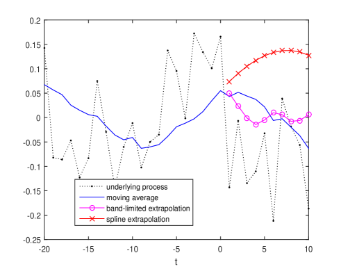
Figure 1: Example of a path $x(t)$, its band-limited extrapolation, its moving average, and piecewise cubic extrapolation with $\Omega=\pi/2$, $N=50$, $h=10$, $\rho=0.2$.

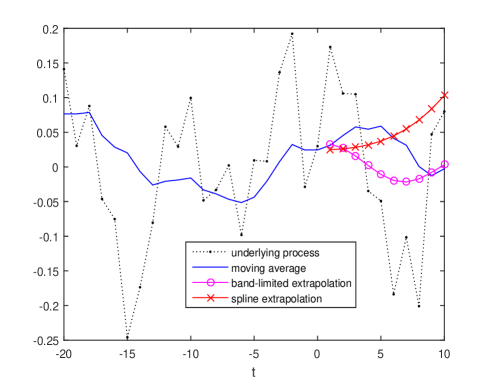
Figure 2: Example of a path $x(t)$, its band-limited extrapolation, its moving average, and shape-preserving piecewise cubic extrapolation with $\nu=8$, $\Omega=\pi/5$, $N=100$, $h=10$, and $\rho=0.4$.

VI-C Estimation of the impact of data truncation

In addition, we did experiments to estimate the impact of truncation for the band-limited extrapolations introduced in Theorem 2. We found that impact of truncation is manageable; it decreases if the size of the sample increasing. In these experiments, we calculated and compared the values

$$\!E_{{\scriptscriptstyle N_{1}},{\scriptscriptstyle N_{2}}}\!=\!\mathbb{E}\!\left[\frac{2\sqrt{\sum_{t=1}^{L}|\widehat{x}_{{\scriptscriptstyle BL},{\scriptscriptstyle N_{1}}}(t)-\widehat{x}_{{\scriptscriptstyle BL},{\scriptscriptstyle N_{2}}}(t)|^{2}}}{\sqrt{\sum_{t=1}^{L}\widehat{x}_{{\scriptscriptstyle BL},{\scriptscriptstyle N_{1}}}(t)^{2}}+\sqrt{\sum_{t=1}^{L}\widehat{x}_{{\scriptscriptstyle BL},{\scriptscriptstyle N_{2}}}(t)^{2}}}\right]$$

describing the impact of the replacement a truncation horizon $N=N_{1}$ by another truncation horizon $N=N_{2}$. Here $\widehat{x}_{{\scriptscriptstyle BL},{\scriptscriptstyle N}}$ is the band-limited extrapolation calculated with truncated data defined by (VI-A) with a truncation horizon $N$; $\mathbb{E}$ denotes again the average over Monte-Carlo experiments.

We used $x(t)$ simulated via (VI.1) with randomly switching ${\rm A}(t)$, the same as in the experiments described above, with the following adjustment for calculation of $E_{{\scriptscriptstyle N_{1}},{\scriptscriptstyle N_{2}}}$. For the case where $N_{2}>N_{1}$, we simulated first a path $x|_{t=-N_{2},...,0}$ using equation (VI.1) with a randomly selected initial value for $z(-N)$ selected at $N=N_{2}$ as was described above, and then used the truncated part $x|_{t=-N_{1},...,0}$ of this path to calculate $\widehat{x}_{{\scriptscriptstyle BL},{\scriptscriptstyle N_{1}}}$; respectively, the path $x|_{t=-N_{2},...,0}$ was used to calculate $\widehat{x}_{{\scriptscriptstyle BL},{\scriptscriptstyle N_{2}}}$.

Table II shows the results of simulations with 10,000 Monte-Carlo trials for each entry and with $\nu=8$, $c=(1,...,1)^{\top}$, $\Omega=\pi/2$, $\rho=0.4$, $L=12$.

TABLE II: Impact of the truncation and the choice of the truncation horizon

$E_{25,50}$	$E_{50,100}$	$E_{100,250}$	$E_{250,500}$	$E_{500,1000}$
0.0525	0.0383	0.0303	0.0180	0.0128

Figure 3 illustrates the results presented in Table II and shows an example of a path $x(t)$ plotted against time $t$ together with the path of its band-limited extrapolations $\widehat{x}_{{\scriptscriptstyle BL},N}(t)$ obtained with the same parameters as for the Table II, with the truncation horizons $N=50$ and $N=100$. The figure shows that the impact of doubling the truncation horizon is quite small, since the paths for extrapolations are quite close.

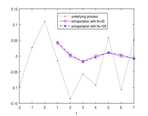
Figure 3: Example of a path $x(t)$ and its band-limited extrapolations $\widehat{x}_{{\scriptscriptstyle BL},N}(t)$ calculated with truncation horizons $N=50$ and $N=100$ in (VI-A).

VII Discussion and future development

The paper suggests a linear equation in the time domain for calculation of band-limited extensions on the future times of band-limited approximations of one-sided semi-infinite sequences representing past observations (i.e. discrete time processes in deterministic setting). The method allows to exclude analysis of processes in the frequency domain and calculation of band-limited approximation of the observed past. This helps to streamline the calculations. Some numerical stability and robustness with respect to input errors and data truncation are established.

It appears that the extrapolation error caused by the truncation is manageable for a short extrapolation horizon and can be significant on a long extrapolation horizon, i.e. for large $t>0$. This is because the components $((A_{N}-A)y_{\rho})(t)$ of the input term in (V) are relatively small for small $t>0$ and can be large for large $t>0$. In particular, this means that long horizon prediction based on this method will not be particularly efficient.

There are possible modifications that we leave for the future research.

In particular, the suggested method can be extended on the setting where $x(t)$ is approximated by a ”high frequency” band-limited processes $\widehat{x}(t)$ such that the process $\widehat{X}\left(e^{i\omega}\right)$ is supported on $[-\pi,-\pi+\Omega]\cup[\pi-\Omega,\pi]$. In this case, the solution follows immediately from the solution given above with $x(t)$ replaced by $(-1)^{t}x(t)$. In addition, processes with more general types of the spectrum gaps on ${\mathbb{T}}$ can be considered, given some modification of the algorithm.

It could be interesting to see if the estimate in Lemma 4 (iv) can be improved; the statement in Lemma 4 (iii) gives a hint that this is estimate is not sharp for preselected $N$.

It could be interesting to apply an iteration method similar to the one used in Zhao2 [31]; see Lemma 1 Zhao2 [31] and citations therein.

Acknowledgment

The author would like thank the anonymous reviewers for the detailed suggestions that improved the manuscript.

References

- Alem eta al [2014] Alem, Y., Khalid, Z., Kennedy, R.A. (2014). Band-limited extrapolation on the sphere for signal reconstruction in the presence of noise, Proc. IEEE Int. Conf. ICASSP’2014, pp. 4141-4145.
- Bingham [2012] Bingham, N. H. (2012). Szegö’s theorem and its probabilistic descendants. Probability Surveys 9, 287-324.
- Almira and Romero [2008] Almira, J.M. and Romero, A.E. (2008). How distant is the ideal filter of being a causal one? Atlantic Electronic Journal of Mathematics 3 (1) 46–55.
- Butzer and Stens [1993] Butzer, P.L. and Stens R.L. (1993). Linear prediction by samples from the past. In: Advanced Topics in Shannon Sampling and Interpolation Theory (R.J. Marks II, ed.), Springer-Verlag, New York, 1993, pp. 157-183.
- Candes et al [2006a] Candés E., Tao, T. (2006), Near optimal signal recovery from random projections: Universal encoding strategies? IEEE Transactions on Information Theory 52(12) (2006), 5406-5425.
- Candes et al [2006b] Candes, E.J., Romberg, J., Tao, T. (2006). Robust uncertainty principles: Exact signal reconstruction from highly incomplete frequency information. IEEE Transactions on Information Theory 52 (2), 489–509.
- Dokuchaev [2010] Dokuchaev, N. (2010). Predictability on finite horizon for processes with exponential decrease of energy on higher frequencies, Signal processing 90 (2) (2010) 696–701.
- Dokuchaev [2010a] Dokuchaev, N. (2012). On predictors for band-limited and high-frequency time series. Signal Processing 92, iss. 10, 2571-2575.
- Dokuchaev [2012b] Dokuchaev, N. (2012). Predictors for discrete time processes with energy decay on higher frequencies. IEEE Transactions on Signal Processing 60, No. 11, 6027-6030.
- Dokuchaev [2016] Dokuchaev, N. (2016). Near-ideal causal smoothing filters for the real sequences. Signal Processing 118, iss. 1, pp. 285-293.
- Dokuchaev [2017] Dokuchaev, N. (2017). On exact and optimal recovering of missing values for sequences. Signal Processing 135, 81–86.
- Ferreira [1994] Ferreira P. G. S. G. (1994). Interpolation and the discrete Papoulis-Gerchberg algorithm. IEEE Transactions on Signal Processing 42 (10), 2596–2606.
- Ferreira [1995] Ferreira P. G. S. G.. (1995a). Nonuniform sampling of nonbandlimited signals. IEEE Signal Processing Letters 2, Iss. 5, 89–91.
- Ferreira [1995b] Ferreira P. G. S. G.. (1995b). Approximating non-band-limited functions by nonuniform sampling series. In: SampTA’95, 1995 Workshop on Sampling Theory and Applications, 276–281.
- Ferreira et al [2007] Ferreira P. J. S. G., Kempf A., and Reis M. J. C. S. (2007). Construction of Aharonov-Berrys superoscillations. J. Phys. A, Math. Gen., vol. 40, pp. 5141–5147.
- Jerri [1977] Jerri, A. (1977). The Shannon sampling theorem - its various extensions and applications: A tutorial review. Proc. IEEE 65, 11, 1565–1596.
- [17] Karnik, S., Zhu, Z., Wakin, M.B., Romberg, J., and Davenport, M.A. (2016) The fast Slepian transform. arXiv:1611.04950.
- Kolmogorov [1941] Kolmogorov, A.N. (1941). Interpolation and extrapolation of stationary stochastic series. Izv. Akad. Nauk SSSR Ser. Mat., 5:1, 3–14.
- Lee and Ferreira [2014] Lee, D.G., Ferreira, P.J.S.G. (2014). Direct construction of superoscillations. IEEE Transactions on Signal processing, V. 62, No. 12,3125-3134.
- Rudin [1987] Rudin, W. Real and Complex Analysis. 3rd ed. Boston: McGraw-Hill, 1987.
- Simon [2011] Simon, B. (2011). Szegö’s Theorem and its descendants. Spectral Theory for perturbations of orthogonal polynomials. M.B. Porter Lectures. Princeton University Press, Princeton.
- Slepian and Pollak [1961] Slepian, D., Pollak, H.O. (1961). Prolates pheroidal wave functions, Fourier analysis and uncertainty-I. Bell Syst.Tech.J. 40, 43–63.
- Slepian and Pollak [1978] Slepian, D. (1978). Prolate spheroidal wave functions, Fourier analysis, and uncertainty. V. The discrete case. Bell Syst. Tech. J. 57, no. 5, 1371-1430.
- [24] Smith, D.A., William F. Ford, W.F., Sidi, A. (1987). Extrapolation methods for vector sequences Siam Review, vol. 29, no. 2, 1987.
- Szegö [1920] Szegö, G. (1920). Beiträge zur Theorie der Toeplitzschen Formen. Math. Z. 6, 167–202.
- Szegö [1921] Szegö, G. (1921). Beiträge zur Theorie der Toeplitzschen Formen, II. Math. Z. 9, 167-190.
- Tzschoppe and Huber [2009] Tzschoppe, R., Huber, J. B. (2009), Causal discrete-time system approximation of non-bandlimited continuous-time systems by means of discrete prolate spheroidal wave functions. Eur. Trans. Telecomm.20, 604–616.
- Wiener [1949] Wiener, N. (1949). Extrapolation, Interpolation, and Smoothing of Stationary Time Series with Engineering Applications, Technology Press MIT and Wiley, New York.
- Yosida [1965] Yosida, K. (1965). Functional Analysis. Springer, Berlin Heilderberg New York.
- [30] Zhao, H., Wang, R., Song, D., Zhang, T., Wu, D. (2014). Extrapolation of discrete bandlimited signals in linear canonical transform domain. Signal Processing 94, 212–218.
- [31] Zhao, H., Wang, R., Song, D., Zhang, T., Liu, Y. (2014). Unified approach to extrapolation of bandlimited signals in linear canonical transform domain. Signal Processing 101, 65–73.