Long-time limit studies of an obstruction in the $g$-function mechanism for semiclassical focusing NLS

Abstract

We consider the long-time properties of the an obstruction in the Riemann-Hilbert approach to one dimensional focusing Nonlinear Schrödinger equation in the semiclassical limit for a one parameter family of initial conditions. For certain values of the parameter a large number of solitons in the system interfere with the $g$-function mechanism in the steepest descent to oscillatory Riemann-Hilbert problems. The obstruction prevents the Riemann-Hilbert analysis in a region in $(x,t)$ plane. We obtain the long time asymptotics of the boundary of the region (obstruction curve). As $t\to\infty$ the obstruction curve has a vertical asymptotes $x=\pm\ln 2$. The asymptotic analysis is supported with numerical results.

1 Introduction

Consider the one dimensional focusing Nonlinear Schrödinger equation (NLS) in the semiclassical limit $\varepsilon\to 0$

$$i\varepsilon q_{t}+\varepsilon^{2}q_{xx}+2\left|q\right|^{2}q=0,\quad t>0$$ (1)

subject to a one parameter family of initial conditions

$$q(x,0,\varepsilon)=A(x)e^{\frac{i\mu}{\varepsilon}S(x)},$$ (2)

where real valued $A(x)$ decays fast as $x\to\pm\infty$ and real valued $S(x)$ converges to $S_{\pm}$ as $x\to\pm\infty$.

This is a well known type of problems of finding the leading asymptotic behavior of the solution $q(x,t,\varepsilon)$ in a singular limit. In the case of the semiclassical focusing NLS (as opposed to the defocusing semiclassical NLS), the problem is known for modulational instability when a smooth initial profile breaks into a seemingly disordered structure.

The first progress in analysis of semiclassical NLS was made by Miller and Kamvissis [22] when in numerical studies they observed some order. This has lead to a number of results [5, 6, 21, 28, 29] based on the Riemann-Hilbert approach to this completely integrable equation. The Riemann-Hilbert approach is based on replacing the nonlinear PDE with a pair of linear operators (Lax pair) first introduced by Lax for KdV equation [20] and later applied to NLS by Zakharov and Shabat [32]. This reformulates the problem for a nonlinear PDE as a scattering/inverse scattering problem for a linear operator. So the asymptotic analysis of the NLS becomes an asymptotic analysis of the spectral data of a linear operator where the initial data for NLS plays the role of a potential. Then the problem is usually further reformulated as a jump (factorization) problem on a contour related to the spectrum of a linear operator - called (oscillatory) Riemann-Hilbert problem (RHP).

Riemann-Hilbert problems are a natural object for the inverse scattering as was noted by Shabat [25] who expressed the hardest step - the inverse scattering as a multiplicative matrix Riemann-Hilbert problem. A (local) RHP we define as the following: find a matrix valued function $m(z)$, which is analytic everywhere in the complex plane except on an oriented contour $\Sigma$, where the function has a prescribed multiplicative matrix jump. Additionally, the function must satisfy a normalization condition at infinity. More precise description of the RH approach can be found in [10, 18]. A simple example of a RHP is the jump matrix to be the identity matrix (”free” case, no jump).

To extract the leading contribution, a $g$-function mechanism was introduced by Deift, Venakides, Zhou [11], applicable to highly oscillatory RHPs. The method is based on factoring out contributions until of the remainder RHP has approximately constant (upto $L_{2}$ correction) jump matrix. Next the ”model” RHP with the constant jumps on finitely many intervals (finite genus) is solved explicitly in terms of Riemann theta functions. Then one needs to show that the remainder ”error” RHP has a small ($L_{2}$) solution. This method can be thought as a nonlinear steepest descent method.

The Riemann-Hilbert approach to asymptotic analysis has a wide range of applications to a diverse array of problems including integrable systems (sine-Gordon, Toda lattice, (m)KdV, (m)NLS, Benjamin-Ono), combinatorics (longest increasing subsequences), Random matrices (GUE, GOE, beta ensembles), and orthogonal polynomials (OPRL, discrete polynomials), to name some.

For NLS a number of initial conditions in the semiclassical limit were analyzed [6, 21, 28, 30]. The leading order solution of NLS was found in terms of Riemann theta functions with underlying Riemann surfaces of finite genus. Other existing results include long time analysis ($\varepsilon=1$) along straight lines $\frac{x}{t}=const$ in the $(x,t)$ plane for several initial data [7, 29]. The analysis was similar and lead to a finite genus ($0$, $1$, and $2$) regions in the $(x,t)$ plane. Key ingredients in all these cases were Lax pair operators, Riemann-Hilbert problems and the $g$-function mechanism.

Consider the one parameter ($\mu\geq 0$) family of initial conditions

$$q(x,0,\varepsilon)=-{\rm sech~{}}(x)\ e^{\frac{i\mu}{\varepsilon}\int_{0}^{x}\tanh sds}.$$ (3)

Even the simplest case $\mu=0$ carries many features and difficulties in the analysis. A common approach is to approximate the initial data without disturbing the leading order of the solution. Moreover, choosing a special sequence $\varepsilon_{n}\to 0$ leads to purely multi-soliton solution which is much simpler for numerical studies. This case was analyzed by Lyng, Miller [21].

For $\mu>0$, the family of initial conditions (3) combines both solitonless initial data for $\mu\geq 2$ as well as radiation in the presence of solitons for $0<\mu<2$. This makes it interesting from the point of view of influence of a large number of solitons.

The solitonless case $\mu\geq 2$ has been analyzed completely for all $x$ and $t>0$ values by Tovbis, Venakides, Zhou in [28]. In the semiclassical limit, the leading order asymptotics is written in terms of Riemann theta functions with parameters $\left\{\alpha_{j}\right\}$ which arise as branchpoints and leading to a Riemann surface. They proved that there is a curve $t=t_{0}(x)$ (called the first break) in the $(x,t)$ plane such that for $0<t<t_{0}(x)$ the leading order of the solution $q(x,t)$ depends only on $\alpha_{0}(x,t)$ and $\alpha_{1}(x,t)=\overline{\alpha}_{0}(x,t)$. This can be seen as a genus $0$ Riemann surface and the asymptotic solution has a WKB type approximation. For $t>t_{0}(x)$ the leading order depends on $\alpha_{0}(x,t)$, $\alpha_{2}(x,t)$, $\alpha_{4}(x,t)$ and their complex conjugates (the genus is 2). In the case of radiation with solitons ($0<\mu<2$) the previous results were partial: only for finite interval of $t$ values (not global in time) [27]. In these studies, there was no information on the region/boundary of rigorous applicability.

In this paper we consider the case $0<\mu<2$ with a similar semiclassical approximation of (3), as it was done in [28]. In these studies the RH approach was completed for finite values of $t$ and was not extendable globally for all $t>0$. The main obstacle for $0<\mu<2$ came from a large number of solitons (order of $O\left(\frac{1}{\varepsilon}\right)$). These solitons correspond to isolated poles of a reflection coefficient of the underlying Lax operator. In the semiclassical limit the isolated singularities accumulate and densely fill an interval in the complex (spectral parameter or energy) plane. This adds significantly to the difficulty of the asymptotic analysis, which breaks as a leading contributing contour coming from analyzing the oscillatory terms in the RHP, collides with these accumulated poles and the error estimates become invalid.

This paper studies the boundary of the region of rigorous applicability of the available asymptotic result. The boundary $t=t_{s}(x)$ (we call it a singular obstruction curve) is a curve in $(x,t)$ plane. We prove that the singular obstruction curve has a vertical asymptotes $x=\pm\ln 2$. We find that the rate at which the singular obstruction curve approaches these asymptotes is $x-\pm\ln 2=O\left(\frac{\ln t}{t}\right)$ as $t\to+\infty$. We also provide the long-time asymptotics of all important quantities including $\alpha_{0}$, $\alpha_{2}$, $\alpha_{4}$. It is conjectured that for $|x|>\ln 2$ the solution maintains genus 2 asymptotics for all $t>t_{0}(x)$ beyond the first break.

The paper is structured as follows: in section 2 we introduce the main object of study - a scalar RHP on $g$-function. In section 3 we obtain the long time limit of the singular obstruction curve. Section 4 provides numerical evidence supporting the asymptotic analysis. In section 5 we discuss the results. Appendix is used for all technical asymptotic computations.

2 g-function problem

Figure 1: Main (bold) and complementary (thin) arcs in the $g$-function problem. The exact positions of the complementary arcs are not fixed.

The $g$-function mechanism was introduced in [11] as a method of extracting the leading order by factoring out an unknown function $g(z)$ and setting up conditions to guarantee that this function gives the leading order. Usually $g(z)$ is defined through conditions on contours in the complex plane. For the semiclassical NLS equation the contour is assumed to be a union of so called ”main” and ”complementary” arcs on which $g(z)$ is defined as the following in the case of genus 2 which is needed for purposes of this paper. General setup of any finite genus is similar [27].

1. Main arcs ($\gamma_{0}$, $\gamma_{m}$):

   $$\left\{\begin{array}[]{ll}g_{+}+g_{-}-f=W&\mbox{on $\gamma_{m}$}\\ g_{+}+g_{-}-f=0&\mbox{on $\gamma_{0}$}\\ \Im(2g_{-}-f)<0&\mbox{right from the main arcs $\gamma_{0}$, $\gamma_{m}$}\\ \Im(2g_{+}-f)<0&\mbox{left from the main arcs $\gamma_{0}$, $\gamma_{m}$}\end{array}\right.$$ (4)

2. Complementary arcs ($\gamma_{c}$):

   $$\left\{\begin{array}[]{lll}g_{+}-g_{-}=\Omega&\mbox{on $\gamma_{c}$}\\ \Im(2g-f)>0&\mbox{on at least one side from $\gamma_{c}$}\\ \end{array}\right.$$ (5)

where $\Omega$, $W\in\mathbb{R}$. The main arcs $\gamma_{0}$, $\gamma_{m}$ form a branch cut structure which defines $g(z)$ [28].

In general, the number of main and complementary arcs is determined for each pair $(x,t)$, where $x$ and $t$ enter in RHP for $g$-function as parameters through $f=f(z,x,t)$. The function $f$ is assumed to be known and it comes from the initial condition (3) through the logarithm of the reflection coefficient $f=\frac{2i}{\varepsilon}\log(r)$.

In this paper we use $f$ obtained by the semiclassical approximation of the initial condition (3) as in [28]

$$f(z,x,t)=\left(\frac{\mu}{2}-z\right)\left[\frac{\pi i}{2}+\ln\left(\frac{\mu}{2}-z\right)\right]+\frac{z+T}{2}\ln\left(z+T\right)+\frac{z-T}{2}\ln\left(z-T\right)$$

$$-T\tanh^{-1}\frac{T}{\mu/2}-xz-2tz^{2}+\frac{\mu}{2}\ln 2,\quad\mbox{when}\ \ \Im z>0,$$ (6)

$$f(z,x,t)=\overline{f(\overline{z},x,t)}\quad\mbox{when}\ \ \Im z<0,$$

where the branch cuts in the logarithms are chosen as the following: from ${\mu\over 2}$ along the real axis to $+\infty$, from $T$ to $0$ and along the real axis to $+\infty$, from $-T$ to $0$ and along the real axis to $-\infty$.

$$f^{\prime}(z,x,t)=-\frac{\pi i}{2}-\ln\left(\frac{\mu}{2}-z\right)+\frac{1}{2}\ln\left(z^{2}-T^{2}\right)-x-4tz,\quad\mbox{when}\ \ \Im z>0.$$ (7)

In the limit to the real axis from the upper half plane $f^{\prime}$ is

$$\Im f^{\prime}(z+i0)=\left\{\begin{array}[]{ll}\frac{\pi}{2},&z<0\\ -\frac{\pi}{2},&0<z<{\mu\over 2}\\ \frac{\pi}{2},&z>{\mu\over 2}\end{array}\right.\quad z\in\mathbb{R}$$ (8)

so $f^{\prime}$ has a jump on the real axis from Schwarz symmetry.

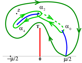
Figure 2: Contours of integration in the upper half plane for $g(z)$, $h(z)$ and $B(z)$ in genus 2. In the lower half plane the contours are symmetric. Large loop contour $\hat{\gamma}$ and the small loop contours $\hat{\gamma}_{m}$, $\hat{\gamma}_{c}$ are shown. For $h(z)$ the point $z$ is inside of $\hat{\gamma}$ and outside of $\hat{\gamma}_{m}$, $\hat{\gamma}_{c}$. For $g(z)$ the point $z$ is outside of $\hat{\gamma}$ and outside of $\hat{\gamma}_{m}$, $\hat{\gamma}_{c}$. For $B(z)$ the point $z$ is inside of $\hat{\gamma}$ and inside of $\hat{\gamma}_{m}$, $\hat{\gamma}_{c}$. As shown, the contours and $z$ suit to compute $h(z)$.

The main and complementary arcs are described by the end points $\{\alpha_{j}\}_{j=0}^{5}$: $\gamma_{0}=\left[\alpha_{1},{\mu\over 2}\right]\cup\left[{\mu\over 2},\alpha_{0}\right]$, $\gamma_{m}=\left[\alpha_{2},\alpha_{4}\right]\cup\left[\alpha_{5},\alpha_{3}\right]$, and $\gamma_{c}=[\alpha_{0},\alpha_{2}]\cup[\alpha_{3},\alpha_{1}]$. Because of the Schwartz symmetry of the problem, $\alpha_{1}=\overline{\alpha}_{0}$, $\alpha_{3}=\overline{\alpha}_{2}$, and $\alpha_{5}=\overline{\alpha}_{4}$. Introduce closed loops $\hat{\gamma}_{0}$, $\hat{\gamma}_{m}$, and $\hat{\gamma}_{c}$ around $\gamma_{0}$, $\gamma_{m}$, and $\gamma_{c}$ respectively. The orientation of these loop contours is clockwise (Fig. 2). The loop $\hat{\gamma}_{0}$ cannot be deformed away from ${\mu\over 2}$ since $f(z)$ is not analytic at $z={\mu\over 2}$. We also introduce a clockwise oriented closed loop $\hat{\gamma}$ enclosing all the main and complementary arcs together. It is also passing through $z={\mu\over 2}$.

The $g$-function have the following expression [28] (Eq.(3.17), (3.18))

$$g(z)=\frac{R(z)}{2\pi i}\left[\oint_{\hat{\gamma}}\frac{f(\xi)}{(\xi-z)R(\xi)}d\xi+\oint_{\hat{\gamma}_{c}}\frac{\Omega}{(\xi-z)R(\xi)}d\xi+\oint_{\hat{\gamma}_{m}}\frac{W}{(\xi-z)R(\xi)}d\xi\right],$$ (9)

where point $z$ lies outside of a large loop $\hat{\gamma}$ and outside of small loops $\hat{\gamma}_{0}$, $\hat{\gamma}_{c}$ and $\hat{\gamma}_{m}$. The factor $R$ is

$$R(\xi)=\sqrt{\left(\xi-\alpha_{0}\right)\left(\xi-\overline{\alpha}_{0}\right)\left(\xi-\alpha_{2}\right)\left(\xi-\overline{\alpha}_{2}\right)\left(\xi-\alpha_{4}\right)\left(\xi-\overline{\alpha}_{4}\right)},$$

where $R(\xi)\sim-\xi^{3}$ as $\xi\to+\infty$ and it has branch cuts along the main arcs $\gamma_{0}$, $\gamma_{m}$. The genus of the Riemann surface of $R(\xi)$ is 2 since $\gamma_{0}$ and $\gamma_{m}$ form three branch cuts.

The constants $W$ and $\Omega$ are solutions to the system:

$$\left(\begin{array}[]{cc}\oint_{\hat{\gamma}_{m}}\frac{1}{R(\xi)}d\xi&\oint_{\hat{\gamma}_{c}}\frac{1}{R(\xi)}d\xi\\ \oint_{\hat{\gamma}_{m}}\frac{\xi}{R(\xi)}d\xi&\oint_{\hat{\gamma}_{c}}\frac{\xi}{R(\xi)}d\xi\end{array}\right)\left(\begin{array}[]{c}W\\ \Omega\end{array}\right)=\left(\begin{array}[]{c}-\oint_{\hat{\gamma}}\frac{f(\xi)}{R(\xi)}d\xi\\ -\oint_{\hat{\gamma}}\frac{\xi f(\xi)}{R(\xi)}d\xi\end{array}\right),$$ (10)

which comes from the requirement $g(z)$ to be analytic at infinity [28].

The branch points $\left\{\alpha_{0},\alpha_{2},\alpha_{4}\right\}$ are computed by solving the system

$$\left\{\begin{array}[]{l}B(\alpha_{0})=0\\ B(\alpha_{2})=0\\ B(\alpha_{4})=0\end{array}\right.,$$ (11)

where

$$B(z)=\oint_{\hat{\gamma}}\frac{f(\xi)}{(\xi-z)R(\xi)}d\xi+\oint_{\hat{\gamma}_{c}}\frac{\Omega}{(\xi-z)R(\xi)}d\xi+\oint_{\hat{\gamma}_{m}}\frac{W}{(\xi-z)R(\xi)}d\xi,$$ (12)

with $z$ being inside of the contours $\hat{\gamma}$, $\hat{\gamma}_{m}$ and $\hat{\gamma}_{c}$ (see Fig. 2).

Additionally the 3 complex branch points satisfy a set of 4 real moment conditions [28]:

$$\oint_{\hat{\gamma}}\frac{\xi^{j}f^{\prime}(\xi)}{R(\xi)}d\xi=0,\quad j=0,1,2,3.$$ (13)

These conditions come from expanding $g^{\prime}(z)$ at infinity into a power series. They are necessary but not sufficient to define $\left\{\alpha_{0},\alpha_{2},\alpha_{4}\right\}$. The system (11) and formula (9) imply (13).

Introduce a convenient notation

$$h(z)=2g(z)-f(z)$$ (14)

then

$$h(z)=\frac{R(z)}{2\pi i}\left[\oint_{\hat{\gamma}}\frac{f(\xi)}{(\xi-z)R(\xi)}d\xi+\oint_{\hat{\gamma}_{c}}\frac{\Omega}{(\xi-z)R(\xi)}d\xi+\oint_{\hat{\gamma}_{m}}\frac{W}{(\xi-z)R(\xi)}d\xi\right],$$

where point $z$ lies inside of a large loop $\hat{\gamma}$ and outside of small loops $\hat{\gamma}_{c}$ and $\hat{\gamma}_{m}$.

Then the $g$-function conditions (4)-(5) are rewritten in terms of $h(z)$ in genus 2:

1. Main arcs ($\gamma_{0}$, $\gamma_{m}$):

   $$\left\{\begin{array}[]{ll}h_{+}+h_{-}=0&\mbox{on $\gamma_{0}$}\\ h_{+}+h_{-}=2W&\mbox{on $\gamma_{m}$}\\ \Im h<0&\mbox{right from $\gamma_{0}$, $\gamma_{m}$}\\ \Im h<0&\mbox{left from $\gamma_{0}$, $\gamma_{m}$}\end{array}\right.$$ (15)

2. Complementary arcs ($\gamma_{c}$):

   $$\left\{\begin{array}[]{lll}h_{+}-h_{-}=2\Omega&\mbox{on $\gamma_{c}$}\\ \Im h>0&\mbox{left or right from $\gamma_{c}$}\end{array}\right.$$ (16)

This suggests the visualization: land ($\Im h>0$), sea ($\Im h<0$), and sea-shore-lines or bridges ($\Im h=0$). A bridge has $\Im h<0$ on both sides while a sea-shore-line has $\Im h>0$ on one side $\Im h<0$ on the other. A main arc can be viewed as a bridge connecting two land regions with sea on both sides. A complementary arc is a land path with exact position being unimportant as long as $\Im h\geq 0$.

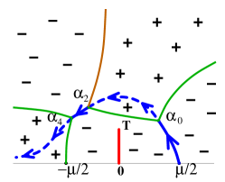
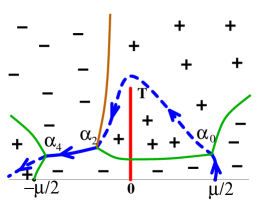
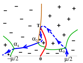
Figure 3: Schematic illustration of the singular obstruction mechanism in the solitons+radiation case ($0<\mu<2$) in the upper half plane. The zero level curve from $\alpha_{2}$ going up touches the top of the branch cut $[0,T]$ and closes the passage to connect $\alpha_{0}$ and $\alpha_{2}$ (dashed).

The so called singular obstruction in the procedure occurs when the above assumptions that there is contour connecting ${\mu\over 2}$ and $-\infty$ consisting of main and complementary arcs exists is invalid. In particular as we show numerical results in Section 4, this scenario occurs at finite values of $t$ for small values of $x$ ($|x|<\ln 2$). One of the complementary arcs collides with the logarithmic branch cut $[0,T]$. More precise assumption on the contours, that there is a path connecting ${\mu\over 2}$ and $-\infty$ along which $\Im h(z)\geq 0$. This condition could fail as shown on Figure 3 for small $x$ values as time increases. We call such curve $x=x_{c}(t)$ in the $(x,t)$ plane the singular obstruction curve defined by the condition

$$\Im h(T,x_{c}(t),t)=0,$$ (17)

where $h(z=T,x,t)$ is understood in the sense of limit:

$$\Im h(T,x,t)=\Im\left(2g(T,x,t)-\lim_{z\to T}f(z,x,t)\right).$$ (18)

Equation (17) is an implicit condition for the singular obstruction curve $x=x_{c}(t)$ which we solve asymptotically below. Numerical investigation suggests that this curve has a vertical asymptote in the $(x,t)$ plane. In the next section we perform asymptotic analysis of the long-time asymptotics of the singular obstruction curve.

3 Long time asymptotic analysis

This section contains the core analysis of the paper. It is devoted to solving of the equation (17) in the long time limit.

Claim 3.1.

In genus 2 in the long time limit the branch points $\alpha_{0}$, $\alpha_{2}$ and $\alpha_{4}$ converge to $\mu/2$, $0$, $-\mu/2$ respectively. Convergence of $\alpha_{0}\to\mu/2$ and $\alpha_{4}\to-\mu/2$ is exponentially fast in $t$ as $t\to\infty$.

For $\mu\geq 2$, the result is proved in [29]. In the case $0<\mu<2$, an additional logarithmic branch cut $[0,T]$ in the upper half plane appears in equations from which $\alpha_{0}$, $\alpha_{2}$, $\alpha_{4}$ are determined. The additional branch cut can be viewed as a small perturbation in the limit $t\to\infty$ and does not affect the leading behavior of the branch points in the claim.

Corollary 3.2.

Claim 3.1 implies that the integrals

$$\int_{{\mu\over 2}}^{\alpha_{0}}\frac{f^{\prime}(\xi)}{(\xi-z)R(\xi)}d\xi,\quad\int_{{\mu\over 2}}^{\overline{\alpha}_{0}}\frac{f^{\prime}(\xi)}{(\xi-z)R(\xi)}d\xi,$$ (19)

$$\int_{\alpha_{4}}^{-{\mu\over 2}}\frac{f^{\prime}(\xi)}{(\xi-z)R(\xi)}d\xi,\quad\int_{\overline{\alpha}_{4}}^{-{\mu\over 2}}\frac{f^{\prime}(\xi)}{(\xi-z)R(\xi)}d\xi$$ (20)

are exponentially small in time as $t\to\infty$.

Proof of Corollary 3.2 is exactly the same as in [29].

Theorem 3.3.

Let $0<\mu<2$. Assuming the genus 2 region in the $(x,t)$ plane allows to send $t$ to infinity, the long time larger solution of the equation

$$\left\{\begin{array}[]{l}\Im h(T,x,t)=0,\\ x>0\end{array}\right.$$

has the following long time asymptotics

$$x(t)=\ln 2-\frac{\left(8ta_{2}+\ln b_{2}\right)b_{2}^{2}}{2|T|^{2}}-C_{3}b_{2}^{2}+O\left(a_{2}b_{2}\right),\ \ \ \ t\to\infty,$$ (21)

where $\alpha_{2}=a_{2}+ib_{2}$, $T=i\sqrt{1-\frac{\mu^{2}}{4}}$, $C_{3}=\frac{1-2\ln|T|}{4|T|^{2}}$ and

$$\left\{\begin{array}[]{l}a_{2}(x,t)=\left.\frac{A_{1}\ln t}{t}+\frac{A_{2}}{t}+\frac{A_{3}\ln t}{t^{2}}+O\left(\frac{1}{t^{2}}\right)\right.\\ b_{2}(x,t)=\frac{B_{1}}{\sqrt{t}}+\frac{B_{2}\ln t}{t^{3/2}}+\frac{B_{3}}{t^{3/2}}+O\left(\frac{\ln t}{t^{5/2}}\right)\end{array},\quad t\to\infty\right.$$ (22)

with

$$\left\{\begin{array}[]{ll}A_{1}=\frac{1}{8},&B_{1}=\frac{\sqrt{\mu}}{2}\\ A_{2}=\frac{1}{4}\ln{\frac{2|T|}{\sqrt{\mu}}}+\frac{\ln 2-x}{4},&B_{2}=\frac{1}{16\sqrt{\mu}}\\ A_{3}=\frac{3}{32\mu},&B_{3}=\frac{2+\ln\frac{2|T|}{\sqrt{\mu}}}{8\sqrt{\mu}}+\frac{\ln 2-x}{8\sqrt{\mu}}\\ \end{array}\right.$$ (23)

or explicitly in terms of $t$

$$x(t)=\ln 2+c_{2}\frac{\ln t}{t}+c_{3}\frac{1}{t}+O\left(\frac{\ln t}{t^{3/2}}\right),\ \ \ \ t\to\infty,$$ (24)

where

$$c_{2}=-\frac{\left(8A_{1}-\frac{1}{2}\right)B_{1}^{2}}{2|T|^{2}}=-\frac{\mu}{16|T|^{2}}$$ (25)

and

$$c_{3}=\left(-\frac{8A_{2}-\ln B_{1}}{2|T|^{2}}-C_{3}\right)B_{1}^{2}=-\frac{\mu\left(1+\ln\frac{4|T|^{2}}{\mu}\right)}{16|T|^{2}}.$$ (26)

Proof:

The proof of the theorem has 4 steps and is presented in the subsections 3.1-3.4.

The following notation

$$\left\{\begin{array}[]{l}a_{j}=\Re(\alpha_{j}),\\ b_{j}=\Im(\alpha_{j})\end{array}\right.$$

will be used throughout the rest of the paper.

3.1 Simplification of $g^{\prime}(z)$.

We start with simplifying the expression for $g^{\prime}(z)$ for $z$ values away from $0$ and $\pm\mu/2$

$$g^{\prime}(z)=\frac{R(z)}{2\pi i}\int_{\gamma_{0}\cup\gamma_{m}}\frac{f^{\prime}(\xi)}{(\xi-z)R_{+}(\xi)}d\xi,$$ (27)

where $z$ is off the main arcs $\gamma_{0}$ and $\gamma_{m}$. To overcome the difficulty of $R$ in the denominator taking near-zero values as the $\alpha_{j}$’s approach the real axis, we transform (27) based on the following simple lemma

Lemma 3.4.

Let $C$ be a closed rectifiable curve in the complex plane. Define

$$G(z)=\int_{C}\frac{F(\xi)}{\xi-z}d\xi,$$ (28)

where $F(z)$ is any continuous (on $C$) function that satisfies the moment condition

$$\int_{C}F(\xi)d\xi=0.$$ (29)

Then

$$G(z)=\frac{1}{z-z_{0}}\int_{C}\frac{(\xi-z_{0})F(\xi)}{(\xi-z)}d\xi,$$ (30)

where $z_{0}$ is off the contour $C$ and $z_{0}\neq z$.

The proof follows from the simple identity

$$\frac{1}{\xi-z}=\frac{\xi-z_{0}}{(z-z_{0})(\xi-z)}-\frac{1}{z-z_{0}},$$ (31)

which together with the moment condition (29), proves the lemma.

First we utilize the moment conditions (13) with the contour of integration placed along the branchcuts $\gamma_{0}\cup\gamma_{m}$

$$\int_{\gamma_{0}\cup\gamma_{m}}\frac{\xi^{k}f^{\prime}(\xi)}{R_{+}(\xi)}d\xi=0,\ \ \ \ \ \ k=0,1,2,3.$$ (32)

These moment conditions can be rewritten in the form

$$\left\{\begin{array}[]{l}\int_{\gamma_{0}\cup\gamma_{m}}\frac{f^{\prime}(\xi)}{R_{+}(\xi)}d\xi=0\\ \int_{\gamma_{0}\cup\gamma_{m}}\frac{\Lambda(\xi)f^{\prime}(\xi)}{R_{+}(\xi)}d\xi=0\\ \int_{\gamma_{0}\cup\gamma_{m}}\frac{\Lambda(\xi)f^{\prime}(\xi)}{R_{+}(\xi)}d\xi=0\\ \int_{\gamma_{0}\cup\gamma_{m}}\frac{\Lambda(\xi)f^{\prime}(\xi)}{R_{+}(\xi)}d\xi=0\end{array}\right.,$$ (33)

where

$$\left\{\begin{array}[]{l}\Lambda(\xi)=\left(\xi-a_{2}\right),\\ \Lambda_{2}(\xi)=\left(\xi-a_{0}\right)\left(\xi-a_{4}\right),\\ \Lambda_{3}(\xi)=\left(\xi-a_{0}\right)\left(\xi-a_{2}\right)\left(\xi-a_{4}\right).\end{array}\right.$$ (34)

Thus by applying Lemma 3.4 to equation (27), we obtain

$$g^{\prime}(z)=\frac{1}{2\pi i}\frac{R(z)}{\Lambda_{3}(z)}\int_{\gamma_{0}\cup\gamma_{m}}\frac{\Lambda_{3}(\xi)f^{\prime}(\xi)}{(\xi-z)R_{+}(\xi)}d\xi.$$ (35)

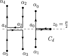
Figure 4: Deformed contour $C_{d}$.

Next we deform the contour of integration to the union of oriented arcs in the upper half plane. Since $f$ in not analytic on the real axis, $a_{0},a_{2},a_{4}$ as points in the complex plane, are understood as limits from the upper half plane: $a_{0}+i0$, $a_{2}+i0$, $a_{4}+i0$. Then $\gamma_{0}\cup\gamma_{m}$ is deformed into

$$\left(\frac{\mu}{2},a_{0}\right)\cup\left(a_{0},a_{0}+ib_{0}\right)\cup\left(a_{2}+ib_{2},a_{2}\right)\cup\left(a_{2},a_{4}\right)\cup\left(a_{4},a_{4}+ib_{4}\right)$$

and its complex conjugate (with the opposite orientation). We call the new contour $C_{d}$ (see Fig. 4). Then

$$g^{\prime}(z)=\frac{1}{2\pi i}\frac{R(z)}{\Lambda_{3}(z)}\int_{C_{d}}\frac{\Lambda_{3}(\xi)f^{\prime}(\xi)}{(\xi-z)R(\xi)}d\xi,$$ (36)

and the moment conditions (33) become

$$\left\{\begin{array}[]{l}\int_{C_{d}}\frac{\Lambda_{2}(\xi)f^{\prime}(\xi)}{R(\xi)}d\xi=0\\ \int_{C_{d}}\frac{\Lambda_{3}(\xi)f^{\prime}(\xi)}{R(\xi)}d\xi=0\end{array}\right..$$ (37)

By Claim 3.1, $\alpha_{0}$ and $\alpha_{4}$ converge to $\pm\mu/2$ exponentially fast in the long time limit. By Corollary 3.2, the contributions from the intervals $\left(\frac{\mu}{2},a_{0}\right)$, $\left(a_{0},a_{0}+ib_{0}\right)$, $\left(a_{4},a_{4}+ib_{4}\right)$ and their conjugates in the contour of integration $C_{d}$ can be neglected, as they are exponentially small as $t\to\infty$, and the interval $(a_{2},a_{4})$ can be replaced with $\left(a_{2},-\frac{\mu}{2}\right)$. Thus (36) reduces to

$$g^{\prime}(z)=\frac{1}{2\pi i}\frac{R(z)}{\Lambda_{3}(z)}\int_{\left(a_{2},-\frac{\mu}{2}\right)\cup\overline{\left(-\frac{\mu}{2},a_{2}\right)}\cup\left(\alpha_{2},\overline{\alpha}_{2}\right)}\frac{\Lambda_{3}(\xi)f^{\prime}(\xi)}{(\xi-z)R(\xi)}d\xi+exp.small,$$ (38)

which, by recalling $f^{\prime}_{+}-f^{\prime}_{-}=\pi i$ on $\left(a_{2},-\frac{\mu}{2}\right)$, transforms into

$$g^{\prime}(z)=\frac{R(z)}{2\Lambda_{3}(z)}\left[\int_{a_{2}}^{-\frac{\mu}{2}}\frac{\Lambda_{3}(\xi)}{(\xi-z)R(\xi)}d\xi+\frac{1}{\pi i}\int_{\alpha_{2}}^{\overline{\alpha}_{2}}\frac{\Lambda_{3}(\xi)f^{\prime}(\xi)}{(\xi-z)R(\xi)}d\xi\right]+exp.small.$$ (39)

Another simplifying observation is

$$\left\{\begin{array}[]{l}\frac{\Lambda_{2}(\xi)}{R(\xi)}=-\frac{1}{\sqrt{\left(\xi-\alpha_{2}\right)\left(\xi-\overline{\alpha}_{2}\right)}}+exp.small\\ \frac{\Lambda_{3}(\xi)}{R(\xi)}=-\frac{\xi-a_{2}}{\sqrt{\left(\xi-\alpha_{2}\right)\left(\xi-\overline{\alpha}_{2}\right)}}+exp.small,\end{array}\right.$$ (40)

Thus, $g^{\prime}(z)$ in terms of real and imaginary parts of $\alpha_{2}=a_{2}+ib_{2}$ is

$$g^{\prime}(z)=-\frac{R(z)}{2\Lambda_{3}(z)}\left[\int_{a_{2}}^{-\frac{\mu}{2}}\frac{(\xi-a_{2})}{(\xi-z)\sqrt{\left(\xi-a_{2}\right)^{2}+b_{2}^{2}}}d\xi\right.$$

$$\left.+\frac{1}{\pi i}\int_{a_{2}+ib_{2}}^{a_{2}-ib_{2}}\frac{(\xi-a_{2})f^{\prime}(\xi)}{(\xi-z)\sqrt{\left(\xi-a_{2}\right)^{2}+b_{2}^{2}}}d\xi\right]+exp.small.$$ (41)

Similarly for the last two moment conditions in (37) we obtain

$$\left\{\begin{array}[]{l}\int_{a_{2}}^{-\frac{\mu}{2}}\frac{1}{\sqrt{\left(\xi-a_{2}\right)^{2}+b_{2}^{2}}}d\xi+\frac{1}{\pi i}\int_{a_{2}+ib_{2}}^{a_{2}-ib_{2}}\frac{f^{\prime}(\xi)}{\sqrt{\left(\xi-a_{2}\right)^{2}+b_{2}^{2}}}d\xi+exp.small=0\\ \int_{a_{2}}^{-\frac{\mu}{2}}\frac{\xi-a_{2}}{\sqrt{\left(\xi-a_{2}\right)^{2}+b_{2}^{2}}}d\xi+\frac{1}{\pi i}\int_{a_{2}+ib_{2}}^{a_{2}-ib_{2}}\frac{(\xi-a_{2})f^{\prime}(\xi)}{\sqrt{\left(\xi-a_{2}\right)^{2}+b_{2}^{2}}}d\xi+exp.small=0\\ \end{array}\right..$$ (42)

The expression for $g^{\prime}(z)$ in (41) and for the moment conditions (42) depend only on $\alpha_{2}=a_{2}+ib_{2}$ and not on $\alpha_{0}$, $\alpha_{4}$. All the dependence on $\alpha_{0}$ and $\alpha_{4}$ is in the exponentially small terms (abbreviated to ”exp.small”).

3.2 Long time asymptotics of the branch point $\alpha_{2}$

We now derive the asymptotics (22). To simplify notations we call $a=a_{2}=o(1)$ and $b=b_{2}=o(1)$. First we change the variable of integration in the second integral in (42) $\xi=by+a$

$$\left\{\begin{array}[]{l}\left.\ln\left(\xi-a+\sqrt{(\xi-a)^{2}+b^{2}}\right)\right|_{a}^{-\frac{\mu}{2}}+\frac{1}{\pi i}\int_{i}^{-i}\frac{f^{\prime}(by+a)}{\sqrt{y^{2}+1}}dy+exp.small=0\\ \left.\sqrt{\left(\xi-a\right)^{2}+b^{2}}\right|_{a}^{-\frac{\mu}{2}}+\frac{1}{\pi i}\int_{i}^{-i}\frac{by\ f^{\prime}(by+a)}{\sqrt{y^{2}+1}}dy+exp.small=0\\ \end{array}\right.$$ (43)

with

$$f^{\prime}(\xi)=-\frac{\pi i}{2}-\ln\left(\frac{\mu}{2}-\xi\right)+\frac{1}{2}\ln\left(\xi^{2}+|T|^{2}\right)-x-4t\xi.$$ (44)

The leading order of $f^{\prime}$ as $t\to\infty$ comes from the last term $-4t\xi$ since $\xi\in[-i,i]$

$$f^{\prime}(by+a)=-4t(by+a)+O(1),$$ (45)

we obtain

$$\left\{\begin{array}[]{l}\ln\left(\sqrt{\left(\frac{\mu}{2}+a\right)^{2}+b^{2}}-\left(\frac{\mu}{2}+a\right)\right)-\ln b+\frac{1}{\pi i}\int_{i}^{-i}\frac{-4t(by+a)}{\sqrt{y^{2}+1}}dy+O(1)=0\\ \sqrt{\left(\frac{\mu}{2}+a\right)^{2}+b^{2}}-b+\frac{1}{\pi i}\int_{i}^{-i}\frac{-4t(by+a)by}{\sqrt{y^{2}+1}}dy+O(b)=0\\ \end{array}\right..$$ (46)

By computing the integral $\int_{i}^{-i}\frac{y}{\sqrt{y^{2}+1}}dy=0$, and expanding the square root for fixed $\mu>0$ and small $a$, $b$.

$$\left\{\begin{array}[]{l}\ln\left(\frac{b}{2(\frac{\mu}{2}+a)}+O(b^{3})\right)-\frac{4ta}{\pi i}\int_{i}^{-i}\frac{1}{\sqrt{y^{2}+1}}dy+O(1)=0\\ \left(\frac{\mu}{2}+a\right)-\frac{4tb^{2}}{\pi i}\int_{i}^{-i}\frac{y^{2}}{\sqrt{y^{2}+1}}dy+O(b)=0\\ \end{array}\right..$$ (47)

Then the integrals are evaluated explicitly $\int_{i}^{-i}\frac{1}{\sqrt{y^{2}+1}}dy=-\pi i$, $\int_{i}^{-i}\frac{y^{2}}{\sqrt{y^{2}+1}}dy=\frac{\pi i}{2}$ and the logarithm is expanded

$$\left\{\begin{array}[]{l}\ln b+4ta+O(1)=0\\ \frac{\mu}{2}-2tb^{2}+O(a+b)=0\\ \end{array}\right..$$ (48)

Solving the second equation for $b$ and plugging the result in the first equation to solve for $a$, we obtain the leading order asymptotics of $\alpha_{2}=a+ib$:

$$\left\{\begin{array}[]{l}a=\frac{\ln t}{8t}+O\left(\frac{1}{t}\right)\\ b=\sqrt{\frac{\mu}{4t}}+O\left(\frac{1}{t}\right)\\ \end{array}\right..$$ (49)

As in the pure radiation case, $\alpha_{2}$ approaches to $0$ on the scale $\frac{1}{\sqrt{t}}$ [29].

Remark 3.5.

The correction term in the second line of (49) is of the order $O\left(\frac{\ln t}{t^{3/2}}\right)$ since in the second equation $O(a+b)$ is in fact $O(a)$ (see (109), (110) in Appendix).

The higher order terms are obtained in the appendix:

$$\left\{\begin{array}[]{l}a=\Re(\alpha_{2})=\frac{1}{8}\frac{\ln t}{t}+A_{2}\frac{1}{t}+A_{3}\frac{\ln t}{t^{2}}+O\left(\frac{1}{t^{2}}\right)\\ b=\Im(\alpha_{2})=\sqrt{\frac{\mu}{4}}\frac{1}{\sqrt{t}}+B_{2}\frac{\ln t}{t^{3/2}}+B_{3}\frac{1}{t^{3/2}}+O\left(\frac{\ln t}{t^{5/2}}\right).\end{array}\right.$$ (50)

This result allows us to compute the long time asymptotics of $g^{\prime}(z)$.

3.3 Long time asymptotics of $g^{\prime}(z)$

Let $z$ be such that its distance $d(z)$ from $\alpha_{0}$ and the interval $[a_{2},a_{4}]$ satisfies $d(z)>>b_{2}$ as $t\to\infty$. First, in (41) we expand $\frac{1}{\xi-z}$ in powers of $\frac{\xi}{z}$. This decomposition uniformly holds away from the branch points $\alpha_{2}$ and $\overline{\alpha}_{2}$, i.e., for $|z|>|\alpha_{2}|$. Then (41) becomes

$$g^{\prime}(z)=\frac{\sqrt{\left(z-a\right)^{2}+b^{2}}}{2(z-a)}\left[\int_{a}^{-\frac{\mu}{2}}\frac{(\xi-a)}{(\xi-z)\sqrt{\left(\xi-a\right)^{2}+b^{2}}}d\xi\right.$$

$$\left.-\frac{1}{\pi iz}\int_{a+bi}^{a-bi}\frac{(\xi-a)f^{\prime}(\xi)}{\sqrt{\left(\xi-a\right)^{2}+b^{2}}}\left(1+\frac{\xi}{z}+\sum_{k=2}^{\infty}\left(\frac{\xi}{z}\right)^{k}\right)d\xi\right]+exp.small.$$ (51)

Taking into account the last moment condition in (42) in the form

$$\frac{1}{\pi i}\int_{a+bi}^{a-bi}\frac{(\xi-a)f^{\prime}(\xi)}{\sqrt{\left(\xi-a\right)^{2}+b^{2}}}d\xi=-\int_{a}^{-\frac{\mu}{2}}\frac{\xi-a}{\sqrt{\left(\xi-a\right)^{2}+b^{2}}}d\xi+exp.small$$ (52)

we arrive at

$$g^{\prime}(z)=\frac{\sqrt{\left(z-a\right)^{2}+b^{2}}}{2(z-a)}\left[\int_{a}^{-\frac{\mu}{2}}\frac{(\xi-a)}{\sqrt{\left(\xi-a\right)^{2}+b^{2}}}\left(\frac{1}{\xi-z}+\frac{1}{z}\right)d\xi\right.$$

$$\left.-\frac{1}{\pi iz}\int_{a+bi}^{a-bi}\frac{(\xi-a)f^{\prime}(\xi)}{\sqrt{\left(\xi-a\right)^{2}+b^{2}}}\left(\frac{\xi}{z}+\sum_{k=2}^{\infty}\left(\frac{\xi}{z}\right)^{k}\right)d\xi\right]+exp.small.$$ (53)

To simplify the expressions, for the rest of this section we reuse (since there is no $\alpha_{0}$, $\alpha_{4}$ dependence anymore) notation $R(z)=-\sqrt{\left(z-a\right)^{2}+b^{2}}$ and $\Lambda(z)=z-a$ in the integrals

$$g^{\prime}(z)=\frac{1}{2}\ \frac{R(z)}{\Lambda(z)}\int_{a}^{-\frac{\mu}{2}}\frac{\Lambda(\xi)}{R(\xi)}\ \frac{\xi}{(\xi-z)z}d\xi$$

$$-\frac{1}{2\pi iz}\ \frac{R(z)}{\Lambda(z)}\int_{a+bi}^{a-bi}\frac{\Lambda(\xi)}{R(\xi)}f^{\prime}(\xi)\left(\frac{\xi}{z}+\sum_{k=2}^{\infty}\left(\frac{\xi}{z}\right)^{k}\right)d\xi+exp.small.$$ (54)

There are two main objects to analyze: $\frac{R(z)}{\Lambda(z)}$ and $\frac{\Lambda(\xi)}{R(\xi)}$. We deal with these ratios separately by a well known trick

$$f_{n}\int g_{n}\ h=(f_{n}-f)\int(g_{n}-g)\ h+(f_{n}-f)\int g\ h+f\int(g_{n}-g)\ h+f\int g\ h.$$ (55)

Using as guidelines, for $t\to\infty$

$$\frac{R(z)}{\Lambda(z)}=-\frac{\sqrt{\left(z-a\right)^{2}+b^{2}}}{z-a}\to-1\quad\mbox{as}\ t\to\infty,$$ (56)

which we think of as $f_{n}\to f$ in (55) and

$$\frac{\Lambda(\xi)}{R(\xi)}=-\frac{\xi-a}{\sqrt{\left(\xi-a\right)^{2}+b^{2}}}\to 1\quad\mbox{in}\ L_{2}\left(a,-{\mu\over 2}\right)\quad\mbox{as}\ t\to\infty,$$ (57)

which plays the role of $g_{n}\to g$.

We do not prove the above statements but rather use them as suggestions in transforming the integrals in (54)

$$g^{\prime}(z)=-\frac{1}{2}\int_{a}^{-\frac{\mu}{2}}\frac{\xi}{(\xi-z)z}d\xi+\frac{1}{2}\left(\frac{R(z)}{\Lambda(z)}+1\right)\int_{a}^{-\frac{\mu}{2}}\frac{\xi}{(\xi-z)z}d\xi$$

$$-\frac{1}{2}\int_{a}^{-\frac{\mu}{2}}\left(\frac{\Lambda(\xi)}{R(\xi)}-1\right)\frac{\xi}{(\xi-z)z}d\xi+\frac{1}{2}\left(\frac{R(z)}{\Lambda(z)}+1\right)\int_{a}^{-\frac{\mu}{2}}\left(\frac{\Lambda(\xi)}{R(\xi)}-1\right)\frac{\xi}{\xi-z}d\xi$$

$$+\frac{1}{2\pi iz}\int_{a+bi}^{a-bi}\frac{\Lambda(\xi)}{R(\xi)}f^{\prime}(\xi)\ \frac{\xi}{z}d\xi-\frac{1}{2\pi iz}\left(\frac{R(z)}{\Lambda(z)}+1\right)\int_{a+bi}^{a-bi}\frac{\Lambda(\xi)}{R(\xi)}f^{\prime}(\xi)\ \frac{\xi}{z}d\xi$$

$$-\frac{1}{2\pi iz}\ \frac{R(z)}{\Lambda(z)}\int_{a+bi}^{a-bi}\frac{\Lambda(\xi)}{R(\xi)}f^{\prime}(\xi)\left(\sum_{k=2}^{\infty}\left(\frac{\xi}{z}\right)^{k}\right)d\xi+exp.small.$$ (58)

For accounting we label these integrals as $I_{1-6}$ and the terms in the last infinite sum of integrals are labeled as $H_{k}$, $k=2,3,...$. We keep terms of the order up to and including $O\left(\frac{1}{t}\right)$. See appendix for detailed calculations of the following result:

$$\left\{\begin{array}[]{l}I_{1}=-\frac{1}{2}\ln\left(-{\mu\over 2}-z\right)+\frac{\mu}{4z}+\frac{1}{2}\ln(-z)+O(a^{2}),\\ I_{2}=\frac{b^{2}}{2z^{2}}I_{1}+O(ab^{2}),\\ I_{3}=\frac{1}{4z^{2}}b^{2}\ln b+\left(\frac{1-2\ln\mu}{8z^{2}}+\frac{\ln\left(1+\frac{\mu}{2z}\right)}{4z^{2}}\right)b^{2}+O(ab),\\ I_{4}=O(b^{4}\ln b)=O\left(\frac{\ln t}{t^{2}}\right),\\ I_{5}=\frac{1}{z^{2}}\left(2tab^{2}-\frac{C_{1}b^{2}}{4}\right)+O(ab),\quad C_{1}=\ln\frac{2|T|}{\mu}-x,\\ I_{6}=O(tab^{4})=O\left(\frac{\ln t}{t^{2}}\right),\\ H_{2}=-\frac{3tb^{4}}{4z^{3}}+O(b^{3}),\\ H_{3}=O(tb^{5})=O\left(\frac{1}{t^{3/2}}\right),\\ H_{k}=O(tb^{k+2})=O\left(\frac{1}{t^{3/2}}\right),\quad k=4,5,\ldots.\end{array}\right.$$ (59)

Recall: $b=O\left(\frac{1}{\sqrt{t}}\right)$ and $a=O\left(\frac{\ln t}{t}\right)$ as $t\to\infty$.

Now putting together these results

$$g^{\prime}(z)=I_{1}+I_{2}+I_{3}+I_{4}+I_{5}+I_{6}+H_{2}+O(H_{3})$$ (60)

$$=I_{1}+O(a^{2})+\frac{b^{2}}{2z^{2}}I_{1}+O(ab^{2})+\frac{1}{4z^{2}}b^{2}\ln b+\left(\frac{1-2\ln\mu}{8z^{2}}+\frac{\ln\left(1+\frac{\mu}{2z}\right)}{4z^{2}}\right)b^{2}$$

$$+O(ab)+O(b^{4}\ln b)+\frac{1}{z^{2}}\left(2tab^{2}-\frac{C_{1}b^{2}}{4}\right)+O(ab)+O(tab^{4})-\frac{3tb^{4}}{4z^{3}}+O(b^{3})=$$ (61)

$$=I_{1}+\frac{1}{4z^{2}}b^{2}\ln b+\frac{2tab^{2}}{z^{2}}-\frac{3tb^{4}}{4z^{3}}$$

$$+\frac{1}{z^{2}}\left(\frac{1}{2}I_{1}+\frac{1-2\ln\mu}{8}+\frac{\ln\left(1+\frac{\mu}{2z}\right)}{4}-\frac{C_{1}}{4}\right)b^{2}+O(ab).$$ (62)

After substitution of the expression for $I_{1}$ and $C_{1}$ the logarithmic terms cancel

$$g^{\prime}(z)=\frac{1}{2}\ln(z)-\frac{1}{2}\ln\left({\mu\over 2}+z\right)+\frac{\mu}{4z}+\frac{1}{z^{2}}\left(\frac{b^{2}\ln b}{4}+2tab^{2}\right)$$

$$+\frac{1}{z^{2}}\left(\frac{1-2\ln|T|}{8}+\frac{x-\ln 2}{4}\right)b^{2}+\frac{1}{z^{3}}\left(-\frac{3tb^{4}}{4}+\frac{\mu b^{2}}{8}\right)+O(ab),$$ (63)

as $t\to\infty$. Note: $O(ab)=O\left(\frac{\ln t}{t^{3/2}}\right)$.

3.4 Long time asymptotics of the singular obstruction curve

In this section we asymptotically solve $\Im h(T,x,t)=0$ which requires asymptotics of $g(z)$. By integrating $g^{\prime}(z)$ to obtain $g(z)$ and using the fact $h(z)=2g(z)-f(z)$ we write

$$g(z)=\int_{r_{0}}^{z}g^{\prime}(s)ds+g(r_{0})$$ (64)

for some $r_{0}\in\mathbb{R}$, $r_{0}\neq{\mu\over 2}$, which implies $\Im g(r_{0})=0$, that is $g(r_{0})$ is real. In particular we can send $r_{0}\to+\infty$ since $g(z)$ is analytic at infinity. Integrating $g^{\prime}$ and evaluating the limit

$$\lim_{r_{0}\to\infty}\left[\frac{1}{2}r_{0}\ln r_{0}-\frac{1}{2}\left(r_{0}+{\mu\over 2}\right)\ln\left(r_{0}+{\mu\over 2}\right)+\frac{\mu}{4}\ln r_{0}\right]$$ (65)

$$=\lim_{r_{0}\to\infty}-\frac{1}{2}\left(r_{0}+{\mu\over 2}\right)\left(\frac{\mu}{2r_{0}}+O\left(\frac{1}{r_{0}^{2}}\right)\right)=-\frac{\mu}{4},$$ (66)

we obtain

$$g(z)=\frac{1}{2}z\ln z-\frac{1}{2}\left(z+{\mu\over 2}\right)\ln\left(z+{\mu\over 2}\right)+\frac{\mu}{4}\ln z-\frac{1}{z}\left(\frac{b^{2}\ln b}{4}+2tab^{2}\right)$$

$$-\frac{1}{z}\left(\frac{1-2\ln|T|}{8}+\frac{x-\ln 2}{4}\right)b^{2}-\frac{1}{2z^{2}}\left(-\frac{3tb^{4}}{4}+\frac{\mu b^{2}}{8}\right)$$

$$+O(ab)+\frac{\mu}{4}+g(\infty).$$ (67)

Then for $0<\mu<2$ and $T=i\sqrt{1-\frac{\mu^{2}}{4}}$

$$\Im g(T)=\frac{1}{2}\Im\left(T+{\mu\over 2}\right)\left[\ln T-\ln\left(T+{\mu\over 2}\right)\right]+\frac{1}{|T|}\left(\frac{b^{2}\ln b}{4}+2tab^{2}\right)$$

$$+\frac{1}{|T|}\left(\frac{1-2\ln|T|}{8}+\frac{x-\ln 2}{4}\right)b^{2}+O(ab).$$ (68)

and the value of $f(T)$ is computed as the limiting value

$$\Im f(T)=\Im\lim_{z\to T}f(z)=\Im\left(\left(\frac{\mu}{2}-T\right)\left[\frac{\pi i}{2}+\ln\left(\frac{\mu}{2}-T\right)\right]\right)+|T|\ln\left(2|T|\right)-x|T|.$$ (69)

Next we compute $\Im h(T)=2\Im g(T)-\Im f(T)$ and after some algebra we arrive at

$$\Im h(T)=|T|(x-\ln 2)+\frac{2}{|T|}\left(\frac{b^{2}\ln b}{4}+2tab^{2}\right)$$

$$+\frac{2}{|T|}\left(\frac{1-2\ln|T|}{8}+\frac{x-\ln 2}{4}\right)b^{2}+O(ab).$$ (70)

Thus the equation

$$\Im h(T,x,t)=0$$ (71)

is asymptotically solved as $t\to\infty$

$$x(t)=\ln 2-\frac{1}{|T|^{2}}\left(\frac{b^{2}\ln b}{2}+4tab^{2}\right)-\left(\frac{1-2\ln|T|}{4|T|^{2}}\right)b^{2}+O(ab),$$ (72)

which proves Theorem 3.3.

Remark 3.6.

An interesting observation that in terms of $\alpha_{2}=a_{2}+ib_{2}$ (50)

$$x(t)=\ln 2+c_{2}\frac{\ln t}{t}+c_{3}\frac{1}{t}+O\left(\frac{\ln t}{t^{3/2}}\right),\ \ \ \ t\to\infty,$$ (73)

where

$$c_{2}=-\frac{\left(8A_{1}-\frac{1}{2}\right)B_{1}^{2}}{2|T|^{2}},\quad\quad c_{3}=\left(-\frac{8A_{2}-\ln B_{1}}{2|T|^{2}}-C_{3}\right)B_{1}^{2}.$$ (74)

To compute $c_{2}$ only $A_{1}$ and $B_{1}$ are needed and to compute $c_{3}$ only $A_{2}$ additionally required. This may indicate that the terms of the order $O\left(\frac{\ln t}{t^{k}}\right)$ and $O\left(\frac{1}{t^{k}}\right)$ could be combined together in computations.

Then our conjecture is that the next terms are of the orders $O\left(\frac{\ln t}{t^{3/2}}\right)$, $O\left(\frac{1}{t^{3/2}}\right)$ and possibly $O\left(\frac{\ln^{2}t}{t^{3/2}}\right)$ in the singular obstruction curve $x(t)$ long time asymptotics. To compute these terms only coefficients: $A_{1}-A_{2}$, $A_{3}-A_{4}$ and $B_{1}$, $B_{2}-B_{3}$ in the asymptotics of $\alpha_{2}(t)$ would be utilized.

4 Numerical computations

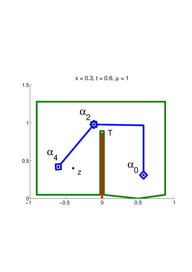
Figure 5: Matlab realization of contours of integration for $h(z)$ in genus 2 (see Fig. 2).

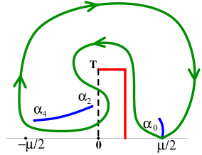
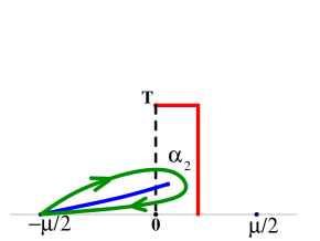
Figure 6: Contours of integration for $h^{\prime}(z)$ in genus 2. Large loop contour $\hat{\gamma}$ is on the left. Simplified contour of integration $\hat{\gamma}_{r}$ for large values of $t$ is on the right.

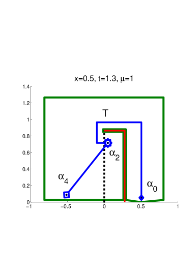
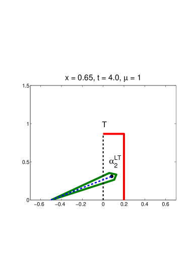
Figure 7: Matlab realization of contours of integration $\hat{\gamma}$ for large $t$ values in genus 2 (left). Matlab realization of contours of integration $\hat{\gamma}_{r}$ for long time computations in genus 2 (right).

4.1 Numerical computation the singular obstruction curve

Figure 8: $\Im h(T,x,t,\mu)$ as a function of time $t$.

As discussed in Section 2 the singular obstruction for a fixed $x$ is defined as one of the roots of the equation

$$\Im h(T,x,t_{s}(x))=0$$ (75)

where the function $\Im h(T,t)$ is a nice function of $t$ (see Fig. 8).

From condition on $z$ being outside of the contour of integration $\hat{\gamma}$, $h(T)$ is not computable directly. Instead

$$\Im h(T)=\Im\left(2g(T)-f(T)\right)=0,$$ (76)

where $f(T)$ is understood as limit, while function $g(z)$ is analytic at $z=T$.

For large $t$ values, the branch point $\alpha_{2}$ approaches the imaginary axis below the point $z=T$ and hits a vertical branch cut $[0,T]$ of function $f$. Using integration on a Riemann surface this event is no special and $\alpha_{2}$ continues moving on another sheet of the Riemann surface without any obstacles.

4.2 Numerical long time computations

Fast convergence of $\alpha_{0}$ and $\alpha_{4}$ to the real axis creates challenges in numerical evaluation of $g$-function for large values of $t$. We modify the computations by incorporating our asymptotic analysis.

The branch points $\alpha_{0}$, $\alpha_{2}$, and $\alpha_{4}$ are singularities of the integrands (in the computation of $h(z)$, $h^{\prime}(z)$, $B(z)$), and need to be encircled by a contour in the upper half plane. This requirement puts the branch points close to the contour of integration causing falling in accuracy. We utilize here that in the genus 2 region $\alpha_{0}$ and $\alpha_{4}$ are exponentially close to $\pm\frac{\mu}{2}$ respectively as $t\to\infty$ and corresponding integrals are exponentially small.

The three complex branch points $\alpha_{0}$, $\alpha_{2}$, and $\alpha_{4}$ satisfy the set of $4$ moment conditions, which are necessary but not sufficient to compute the $\alpha$’s:

$$\left\{\begin{array}[]{l}\oint_{\hat{\gamma}}\frac{f^{\prime}(\xi)}{R(\xi)}d\xi=0\\ \oint_{\hat{\gamma}}\frac{\xi f^{\prime}(\xi)}{R(\xi)}d\xi=0\\ \oint_{\hat{\gamma}}\frac{\xi^{2}f^{\prime}(\xi)}{R(\xi)}d\xi=0\\ \oint_{\hat{\gamma}}\frac{\xi^{3}f^{\prime}(\xi)}{R(\xi)}d\xi=0,\end{array}\right.$$ (77)

where

$$R(\xi)=\sqrt{\left(\xi-\alpha_{0}\right)\left(\xi-\overline{\alpha}_{0}\right)\left(\xi-\alpha_{2}\right)\left(\xi-\overline{\alpha}_{2}\right)\left(\xi-\alpha_{4}\right)\left(\xi-\overline{\alpha}_{4}\right)}.$$ (78)

with the branch cuts chosen along the main arcs: $\left[{\mu\over 2},\alpha_{0}\right]$, $\left[\alpha_{2},\alpha_{4}\right]$ and their complex conjugates.

By considering linear combinations of the moment conditions (77), the last two of these conditions can be written as

$$\left\{\begin{array}[]{l}\oint_{\hat{\gamma}}\frac{\left(\xi-{\mu\over 2}\right)\left(\xi+{\mu\over 2}\right)f^{\prime}(\xi)}{R(\xi)}d\xi=0\\ \oint_{\hat{\gamma}}\frac{\xi\left(\xi-{\mu\over 2}\right)\left(\xi+{\mu\over 2}\right)f^{\prime}(\xi)}{R(\xi)}d\xi=0.\end{array}\right.$$ (79)

Since $\alpha_{0}\to{\mu\over 2}$ and $\alpha_{4}\to-{\mu\over 2}$, we modify the contour of integration accordingly. The large loop $\hat{\gamma}$ is reduced to a smaller loop around $\left[-{\mu\over 2},\alpha_{2}\right]$ and its complex conjugate which we call $\hat{\gamma}_{r}$ (see Fig 6). This leads to improvement of speed and stability and simplifies the system (79)

$$\left\{\begin{array}[]{l}\oint_{\hat{\gamma}_{r}}\frac{\left(\xi-{\mu\over 2}\right)\left(\xi+{\mu\over 2}\right)f^{\prime}(\xi)}{R(\xi)}d\xi+exp.small=0\\ \oint_{\hat{\gamma}_{r}}\frac{\xi\left(\xi-{\mu\over 2}\right)\left(\xi+{\mu\over 2}\right)f^{\prime}(\xi)}{R(\xi)}d\xi+exp.small=0,\end{array}\right.$$ (80)

where

$$R(\xi)=\left(\xi-{\mu\over 2}\right)\left(\xi+{\mu\over 2}\right)\sqrt{\left(\xi-\alpha_{2}\right)\left(\xi-\overline{\alpha}_{2}\right)}$$ (81)

with the branch cut chosen to connect $\alpha_{2}$ and $\overline{\alpha}_{2}$ through $-{\mu\over 2}$. After cancelations, the moment conditions (80) look similar to the case of genus 0 with one unknown branch point $\alpha_{2}$. All dependence on $\alpha_{0}$ and $\alpha_{4}$ is in the exponentially small terms. Then we approximate $\alpha_{2}$ with $\alpha_{2}^{LT}$ which satisfies a system of two real equations

$$\left\{\begin{array}[]{l}\oint_{\hat{\gamma}_{r}}\frac{f^{\prime}(\xi)}{R_{LT}(\xi)}d\xi=0\\ \oint_{\hat{\gamma}_{r}}\frac{\xi f^{\prime}(\xi)}{R_{LT}(\xi)}d\xi=0,\end{array}\right.$$ (82)

where

$$R_{LT}(\xi)=\sqrt{\left(\xi-\alpha_{2}^{LT}\right)\left(\xi-\overline{\alpha}_{2}^{LT}\right)}$$ (83)

with the branch cut chosen to connect $\alpha_{2}^{LT}$ and $\overline{\alpha}_{2}^{LT}$ through $-{\mu\over 2}$.

One of the key advantages of these long time computations is increased speed in exchange of precision in computing $\alpha_{2}$. Solving the full system of $B$-function equations (11) for $\alpha_{0}$, $\alpha_{2}$, and $\alpha_{4}$ involves computing and inverting a $6$x$6$ matrix of partial derivatives for each iteration. While the long time approximations of $\alpha_{2}^{LT}$ by solving (82) involve computing and inverting a $2$x$2$ matrix of partial derivatives.

Using the same contour reduction, we compute $h^{\prime}(z)$ in genus 2 for large $t$ values

$$h_{LT}^{\prime}(z)=\frac{R_{LT}(z)}{2\pi i}\oint_{\hat{\gamma}_{r}}\frac{f^{\prime}(\xi)}{(\xi-z)R_{LT}(\xi)}d\xi.$$ (84)

Long-time computations of $\Im h(z)$ in genus 2 as

$$\Im h_{LT}(T)=\Im\int_{r_{0}}^{z}h^{\prime}_{LT}(s)ds,$$ (85)

where $r_{0}$ is some real number.

Long time computations of the singular obstruction curve are based on long time computations of $\alpha_{2}^{LT}(t)$ and $\Im h_{LT}(z)$. First, $\alpha_{2}^{LT}(t)$ is computed which is used to evaluate $\Im h_{LT}(T,\alpha_{2}^{LT},t)$. The long-time approximation of the singular obstruction $t_{s}^{LT}(x)$ then computed from

$$\Im h_{LT}\left(T,\alpha_{2}^{LT}\left(t_{s}^{LT}\right),t_{s}^{LT}\right)=0.$$ (86)

Using our long time computations of $\alpha_{2}^{LT}$, $h^{\prime}_{LT}(z)$, and $\Im h_{LT}(z)$ we avoid the mentioned above difficulties with accuracy and improve the speed of the computations in the case of $\alpha_{2}^{LT}$ and $h^{\prime}_{LT}(z)$.

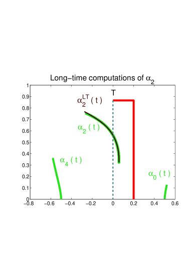
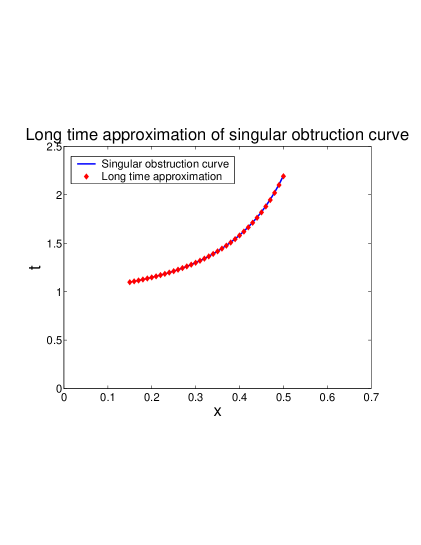
Figure 9: Approximation of $\alpha_{2}(t)$ with $\alpha_{2}^{LT}(t)$ for $x=1.0$, $\mu=1$ in genus 2 (left). Approximation of the singular obstruction $t_{s}(x)$ with $t_{s}^{LT}(x)$ for $\mu=1$ in genus 2 (right).

The long time approximation $\alpha_{2}^{LT}$ of the correct value of $\alpha_{2}$ as a function of time $t$ are presented in Figure 9 (left). It shows the time evolution of $\alpha_{0}$, $\alpha_{2}$, $\alpha_{4}$ and $\alpha_{2}^{LT}$ for $x=1.0$ and $\mu=1$. $\alpha_{2}$ and $\alpha_{2}^{LT}$ demonstrate similar and converging trajectories. The difference convergence tends to zero as $t$ increases.

The long time approximation $t_{s}^{LT}(x)$ of the singular obstruction curve $t=t_{s}(x)$ for $\mu=1$ is presented in Figure 9 (right). It demonstrates good agreement for $t$ values as low as $1$.

5 Discussion

5.1 First break

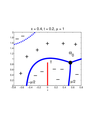
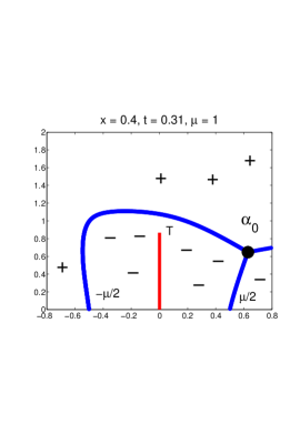
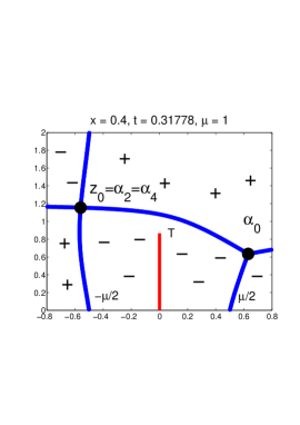
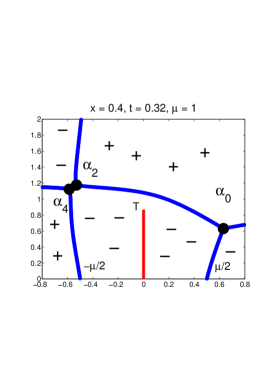
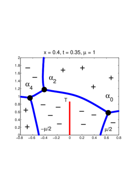
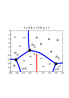
Figure 10: Mechanism of the first break: $t$ evolution of the zero level curves of $\Im h$ for $x=0.4$, $\mu=1$. This sequence illustrates the birth of the main arc $[\alpha_{2},\alpha_{4}]$.

The first break of the asymptotic solution of NLS (1) with the initial conditions (3) in the semiclassical limit $\varepsilon\to 0$ was analytically studied by Tovbis, Venakides, and Zhou in [28]. They established the mechanism of the first break for the $\mu>0$ analytically as time $t$ evolution process. From $t=0$, as $t$ increases the genus changes from $0$ to $2$ with a new main arc $[\alpha_{2},\alpha_{4}]$ created in the upper half plane. In the present work we support their proof numerically.

Figure 10 illustrates the mechanism of the first break from the point of view of the branch points $\alpha$’s and zero level curves of $\Im h$. First, for small $t$ the genus is 0 and there is only one branch point in the upper half plane $\alpha_{0}$. Then, a new pair of branch points $[\alpha_{2},\alpha_{4}]$ is created, while $\alpha_{0}$ continues to approach ${\mu\over 2}$ under a modified trajectory.

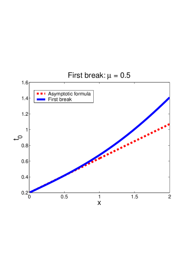
Figure 11: First breaking curve $t_{0}(x)$ (solid) and its small $x$ asymptotics (87) (dashed).

The asymptotic behavior of the first breaking curve in the large and small $x$ limits for $\mu\geq 2$ was established in [28] and [29]

$$t_{0}(x)=\left\{\begin{array}[]{l}\frac{1}{2(\mu+2)}+\frac{\cot\frac{\pi}{5}}{2\sqrt{\mu+2}}x+O\left(x^{3/2}\right),\quad x\to 0\\ \frac{x}{2\mu}-\frac{1}{\mu}\ln\frac{2\mu}{\mu+2T}-\frac{T/\mu}{\mu+2T}+O\left(\frac{1}{x}\right),\quad x\to\infty\end{array}\right..$$ (87)

In the soliton+radiation case $0<\mu<2$ the above large $x$ asymptotic expression produces complex answers. Our conjecture is that the above expression is correct if one substitutes $T=0$. This conjecture is based on the comparison of our our leading order term in the long time limit of $\alpha_{2}$ (22) with the leading term in the expression above (1.5) in [29] for $\mu\geq 2$.

The small $x$ asymptotics in (87) is proved to be valid [28] for $0<\mu<2$. Figure 11 demonstrates agreement of the first breaking curve with the small $x$ asymptotic formula.

In this case, the first break is a boundary between genus 0 and genus 2 regions. From the point of view of genus 2, the first break is a singular event of colliding of two branch points $\alpha_{2}$ and $\alpha_{4}$ with the main arc $[\alpha_{2},\alpha_{4}]$ reducing to a point. Numerically we observed this phenomenon in $x$, $t$ and $\mu$ evolutions. Figure 13 demonstrates how the choice of parameters $x$ and $t$ for the branch points $\alpha_{0}$, $\alpha_{2}$, $\alpha_{4}$ evolution correspond to the first breaking curves.

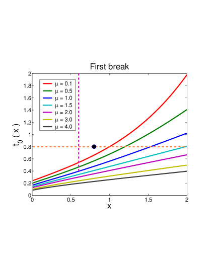
Figure 12: First breaking curves: $t_{0}(x)$ for several $\mu$ values (left), $t_{0}(\mu)$ for several $x$ values (right).

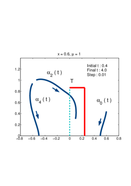
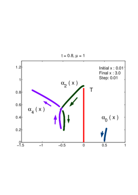
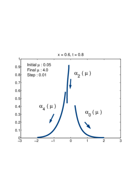
Figure 13: Time $t$ (left), space $x$ (middle), and parameter $\mu$ (right) evolution of the branch points $(\alpha_{0},\alpha_{2},\alpha_{4})$ in genus 2. Collision of $\alpha_{2}$ and $\alpha_{4}$ corresponds to the first break.

The vertical dashed line on Figure 12 (left picture) at $x=0.6$ represents the $t$ evolution for $\mu=1$ in Fig. 13 (left picture). The line starts above the first breaking curve for $\mu=1$ so the branch points $\alpha_{2}$ and $\alpha_{4}$ do not collide.

The horizontal dashed line on Figure 12 (left picture) $t=0.8$ shows the $x$ evolution for $\mu=1$ in Fig. 13 (middle picture). This line intersects the first breaking curve at $x\approx 1.5$.

The big black dot at $x=0.8$, $t=0.8$ represents the parameters for the $\mu$ evolution in Figure 13 (right picture). The dot is located in genus 2 region above all the breaking curves which is confirmed by $\alpha$’s trajectories without collisions for $\mu$ values between $0.05$ and $4.0$.

Finally, we look at the first break as a function of the parameter $\mu$. Figure 14 shows no sign of loss of smoothness at $\mu=2$ which is a critical value for existence of solitons in the initial conditions (3). This dependence is investigated in more details in [1].

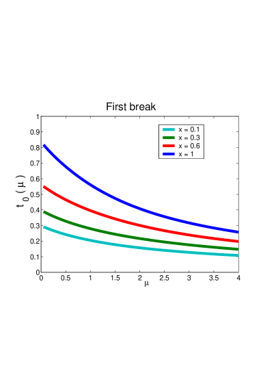
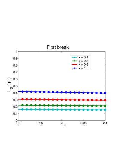
Figure 14: First breaking curves $t=t_{0}(\mu)$ for several $x$ values.

5.2 Singular obstruction

The mechanism for the singular obstruction is a collision of a branch of zero level curves with the logarithmic branch point $T$ (see Fig. 15). This collision closes the passage between $\alpha_{0}$ and $\alpha_{2}$ around the logarithmic branch cut $[0,T]$ and invalidates error estimates. Formally all the expressions $h^{\prime}(z)$, $h(z)$ are correct as solutions of RH problems however the underlying assumptions are not valid: in Figure 15 (right picture) there is no path to connect ${\mu\over 2}$ with $-\infty$ satisfying $\Im h\geq 0$ which is necessary to guarantee capturing the leading order of the asymptotic solution of NLS.

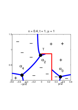
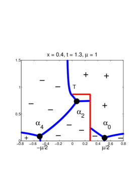
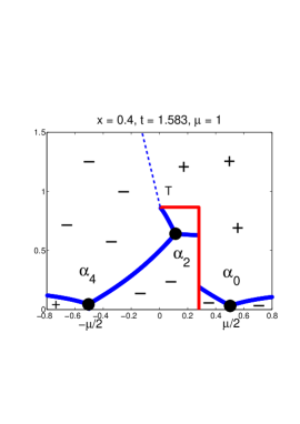
Figure 15: Mechanism of the singular obstruction: time evolution of the zero level curves of $\Im h$ for $x=0.4$, $\mu=1$ in genus 2.

It is not clear at this point how to extend the function $h(z)$ beyond the singular obstruction. However, the term ”singular obstruction” symbolizes the difficulties of the asymptotic analysis rather than drastic changes in the solution. The main difficulty is to extend a Riemann surface continuously after a collision of a zero level curve with a logarithmic branch point singularity.

In this paper we confirm numerically existence of the singular obstruction and compute two correction terms in the long time limit.

$$x=\ln 2+c_{2}\frac{\ln t}{t}+c_{3}\frac{1}{t}+O\left(\frac{\ln t}{t^{3/2}}\right),\ \ \ \ t\to\infty,$$ (88)

where

$$c_{2}=-\frac{\mu}{16|T|^{2}},\quad\quad c_{3}=-\frac{\mu\left(1+\ln\frac{4|T|^{2}}{\mu}\right)}{16|T|^{2}},$$ (89)

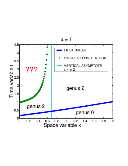
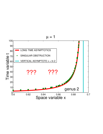
Figure 16: Singular obstruction curve $t=t_{s}(x)$ and first breaking curve $t_{0}(x)$ for $\mu=1$ are on the left. The long time asymptotics of the singular obstruction curve (88) and the long time computations of the singular obstruction curve $t=t_{s}^{LT}(x)$ are on the right.

Comparison of the long time computations of the singular obstruction with the asymptotic formula (24) is given in Figure 16 (right picture).

Based on numerical evidence, our conjecture that the singular obstruction exists only for a finite interval $[0,\ln 2)$ and the location of the vertical asymptote is independent of $\mu$.

From the asymptotic analysis of $\Im h(T,t)$ as a function of $t$ in (70),

$$\Im h(T,t)=|T|(x-\ln 2)+o(1),\quad t\to\infty.$$ (90)

So $\Im h(T,t)$ has a horizontal asymptote $|T|(x-\ln 2)$ as $t\to\infty$.

Figure 8 suggests that for $x>\ln 2$ function $\Im h(T,t)$ has only one root while the other root corresponding to the singular obstruction is not present. This conjecture is supported by the asymptotics of $\Im h(T,t)$ which is asymptotically strictly positive for $x>\ln 2$ for all $t$ large enough.

There is no numerical evidence of any other breaks to occur before the singular obstruction. It is an open question how to extend the current asymptotics beyond the singular obstruction curve. More constructively, this is a question of the new genus of the Riemann surface after collision of the zero level curve with a logarithmic branch point.

Calculations by Lyng, Miller [21] in the case $\mu=0$ suggest that after the second break the genus is 4. However, they are using a somewhat different approach of changing the RHP by adjusting the reflection coefficient. Effectively, they are changing approximations of $f(z)$ on the fly: for some region in the $(x,t)$ plane they are using the same $f(z)$ as we are, while for other regions they are considering a different approximation of $f(z)$ (different approximation of the reflection coefficient at later $t$ values) and consequently a different RHP. This seems to be equivalent to dealing with two $f$-functions at the same time or dealing with two sheets of the Riemann surface at the same time.

Our analysis is based on approximating $f(z)$ at $t=0$ upto order $O(\varepsilon)$ and use this approximation for all $t>0$. It is possible that the leading terms in the used approximation of $f(z)$ as $\varepsilon\to 0$, do not contain information about the second break. Thus taking into account correction terms of the order $O(\varepsilon)$ and $O(\varepsilon^{2})$ is another approach to describing the second break.

6 Appendix

6.1 Higher order terms of $a_{2}$, $b_{2}$ in Theorem 3.3

In this section we compute higher order terms in the asymptotics of $\alpha_{2}=a_{2}+ib_{2}$ in the long time limit from the couple of moment conditions (42).

6.1.1 Simplification of the first moment condition (42)

Consider the first moment condition with the exponentially small terms dropped

$$\int_{a}^{-\frac{\mu}{2}}\frac{1}{\sqrt{\left(\xi-a\right)^{2}+b^{2}}}d\xi+\frac{1}{\pi i}\int_{a+ib}^{a-ib}\frac{f^{\prime}(\xi)}{\sqrt{\left(\xi-a\right)^{2}+b^{2}}}d\xi=O\left(\frac{1}{t^{2}}\right).\\$$ (91)

As it was shown above, $a=O\left(\frac{\ln t}{t}\right)$ and $b=O\left(\frac{1}{\sqrt{t}}\right)$ as $t\to\infty$. Our goal is to compute the next two terms of asymptotics of $a$ and $b$. First, we compute the first integral explicitly and make a change of variables in the second integral $\xi=by+a$

$$\left.\ln\left(\xi-a+\sqrt{(\xi-a)^{2}+b^{2}}\right)\right|_{a}^{-\frac{\mu}{2}}+\frac{1}{\pi i}\int_{i}^{-i}\frac{f^{\prime}(by+a)}{\sqrt{y^{2}+1}}dy=O\left(\frac{1}{t^{5}}\right).$$ (92)

Since both $a$ and $b$ are small, to estimate the integral we decompose $f^{\prime}(\xi)$ in Taylor series near $\xi=0$ while isolating the term containing $t$ explicitly

$$f^{\prime}(\xi)=-4t\xi+f^{\prime}(0)+(f^{\prime\prime}(0)+4t)\xi+\frac{f^{\prime\prime\prime}(0)}{2}\xi^{2}+O(\xi^{3}).$$ (93)

Next, we incorporate Schwartz reflection symmetry $f^{\prime}\left(\overline{\xi}\right)=\overline{f^{\prime}(\xi)}$ and the fact that all $f^{(k)}(0)$ are real for $k\geq 2$, then

$$f^{\prime}(by+a)=-4t(by+a)+C_{1}+iC_{2}\mbox{sign}\left(\frac{y}{i}\right)+C_{3}(by+a)+C_{4}(by+a)^{2}+O((by+a)^{3}),$$ (94)

where the constants $C_{j}$ are obtained from (44) as limiting values

$$f^{(j)}(0)=\lim_{\varepsilon\to 0^{+}}(f^{(j)}(0+i\varepsilon)).$$ (95)

So

$$\left\{\begin{array}[]{l}C_{1}=\ln\frac{2|T|}{\mu}-x\\ C_{2}=\frac{\pi}{2}\\ C_{3}=\frac{2}{\mu}\end{array}\right..$$ (96)

After plugging (94) and (96) back in (92) one obtains

$$\ln\left(\sqrt{\left(\frac{\mu}{2}+a\right)^{2}+b^{2}}-\left(\frac{\mu}{2}+a\right)\right)-\ln b+\frac{1}{\pi i}\int_{i}^{-i}\frac{-4t(by+a)}{\sqrt{y^{2}+1}}dy$$

$$+\frac{1}{\pi i}\int_{i}^{-i}\frac{C_{1}+iC_{2}\mbox{sign}\left(\frac{y}{i}\right)+C_{3}(by+a)+C_{4}(by+a)^{2}+O((by+a)^{3})}{\sqrt{y^{2}+1}}dy=0,$$ (97)

where after expanding all the terms, using symmetries in the integrals, and only keeping terms upto order $O(b^{2})=O\left(\frac{1}{t}\right)$, we see

$$\ln\left(\frac{b}{2(\frac{\mu}{2}+a)}+O(b^{3})\right)+\frac{1}{\pi i}\int_{i}^{-i}\frac{-4ta+C_{1}+C_{3}a}{\sqrt{y^{2}+1}}dy+O(b^{2})=0,$$ (98)

which simplifies to

$$\ln\left(\frac{b}{2(\frac{\mu}{2}+a)}\right)-(-4ta+C_{1}+C_{3}a)+O(b^{2})=0$$ (99)

and its final form is

$$\ln b+4ta-C_{1}-\ln\mu+\left(-\frac{2}{\mu}-C_{3}\right)a+O(b^{2})=0.$$ (100)

Finally, we plug in values of $C_{1}$ and $C_{3}$ from (96)

$$\ln b+4ta+x-\ln 2|T|-\frac{4a}{\mu}+O(b^{2})=0.$$ (101)

In order to extract the asymptotics of $a$ and $b$ from this equation we need to couple it with the other moment condition.

6.1.2 Simplification of the second moment condition (42)

Consider

$$\int_{a}^{-\frac{\mu}{2}}\frac{\xi-a}{\sqrt{\left(\xi-a\right)^{2}+b^{2}}}d\xi+\frac{1}{\pi i}\int_{a+ib}^{a-ib}\frac{(\xi-a)f^{\prime}(\xi)}{\sqrt{\left(\xi-a\right)^{2}+b^{2}}}d\xi=0.$$ (102)

In a similar manner as for the other moment condition, we evaluate the first integral and make a change of variables $\xi=by+a$ in the second integral

$$\sqrt{\left(\frac{\mu}{2}+a\right)^{2}+b^{2}}-b+\frac{1}{\pi i}\int_{i}^{-i}\frac{byf^{\prime}(by+a)}{\sqrt{y^{2}+1}}dy=0.$$ (103)

Next, we compute the integral by expanding $f^{\prime}(\xi)$ into Taylor series (94)

$$\int_{i}^{-i}\frac{byf^{\prime}(by+a)}{\sqrt{y^{2}+1}}dy$$ (104)

$$=\int_{i}^{-i}\frac{by\left[-4t(by+a)+C_{1}+iC_{2}\mbox{sign}\left(\frac{y}{i}\right)+C_{3}(by+a)+C_{4}(by+a)^{2}+O((by+a)^{3})\right]}{\sqrt{y^{2}+1}}dy.$$ (105)

and using the symmetry in the integral which make many of the terms to disappear

$$=\left(-4tb^{2}+C_{3}b^{2}\right)\int_{i}^{-i}\frac{y^{2}}{\sqrt{y^{2}+1}}dy+2C_{2}bi\int_{i}^{0}\frac{y}{\sqrt{y^{2}+1}}dy+O(ab^{2})$$ (106)

$$=\left(-4tb^{2}+C_{3}b^{2}\right)\frac{\pi i}{2}+2C_{2}bi+O\left(ab^{2}\right).$$ (107)

Then the equation (103) reads

$$\sqrt{\left(\frac{\mu}{2}+a\right)^{2}+b^{2}}-b-2tb^{2}+\frac{C_{3}b^{2}}{2}+\frac{2C_{2}b}{\pi}+O\left(ab^{2}\right)=0$$ (108)

and after expanding the square root

$$\frac{\mu}{2}-2tb^{2}+\left(\frac{2C_{2}}{\pi}-1\right)b+a+\left(\frac{1}{\mu}+\frac{C_{3}}{2}\right)b^{2}+O\left(ab^{2}\right)=0.$$ (109)

This equation is an extended version of the second equation in (48). After substituting expressions for $C_{2}$ and $C_{3}$ from (96) we see that the term of order the $O(b)$ vanishes

$$\frac{\mu}{2}-2tb^{2}+a+\frac{2b^{2}}{\mu}+O\left(ab^{2}\right)=0.$$ (110)

6.1.3 Asymptotically solving the system of moment conditions (42)

We want to solve the system of two asymptotic equations for $a$ and $b$

$$\left\{\begin{array}[]{l}\ln b+4ta+x-\ln 2|T|-\frac{4a}{\mu}+O(b^{2})=0\\ \frac{\mu}{2}-2tb^{2}+a+\frac{2b^{2}}{\mu}+O\left(ab^{2}\right)=0,\end{array}\right.$$ (111)

where as we established in (49) the leading order solutions are

$$\left\{\begin{array}[]{l}a=\frac{\ln t}{8t}+O\left(\frac{1}{t}\right)\\ b=\sqrt{\frac{\mu}{4t}}+O\left(\frac{1}{t}\right).\end{array}\right.$$ (112)

We find the correction terms by writing

$$\left\{\begin{array}[]{l}a=\frac{\ln t}{8t}+\frac{\varepsilon_{1}\ln t}{t}\\ b=\sqrt{\frac{\mu}{4t}}+\frac{\delta_{1}}{\sqrt{t}}\end{array}\right.$$ (113)

with functions $\varepsilon_{1}$, $\delta_{1}$ to be determined. Then

$$\left.\begin{array}[]{l}\ln b=-\frac{1}{2}\ln t+\ln\sqrt{\frac{\mu}{4}}+O(\delta_{1})\\ b^{2}=\frac{\mu}{4t}+\frac{\sqrt{\mu}\delta_{1}}{t}+\frac{\delta_{1}^{2}}{t},\end{array}\right.$$ (114)

which we substitute into (111) and obtain

$$\left\{\begin{array}[]{l}-\frac{1}{2}\ln t+\ln\sqrt{\frac{\mu}{4}}+O(\delta_{1})+\frac{1}{2}\ln t+4\varepsilon_{1}\ln t+x-\ln 2|T|+O(a)=0\\ \frac{\mu}{2}-\frac{\mu}{2}-2\sqrt{\mu}\delta_{1}-2\delta_{1}^{2}+\frac{\ln t}{8t}+\frac{\varepsilon_{1}\ln t}{t}+O\left(b^{2}\right)=0.\end{array}\right.$$ (115)

This leads to the following asymptotic equations

$$\left\{\begin{array}[]{l}4\varepsilon_{1}\ln t+\ln\sqrt{\frac{\mu}{4}}+x-\ln 2|T|+O(\delta_{1})+O(a)=0\\ -2\sqrt{\mu}\delta_{1}+\frac{\ln t}{8t}+O\left(\frac{\varepsilon_{1}\ln t}{t}\right)+O\left(b^{2}\right)+O(\delta_{1}^{2})=0,\end{array}\right.$$ (116)

which we solve for $\varepsilon_{1}$ and $\delta_{1}$

$$\left\{\begin{array}[]{l}\varepsilon_{1}=-\frac{\ln\sqrt{\frac{\mu}{4}}+x-\ln 2|T|}{4\ln t}+O\left(\frac{1}{t}\right)\\ \delta_{1}=\frac{\ln t}{16\sqrt{\mu}t}+O\left(\frac{1}{t}\right)\end{array}\right.$$ (117)

and thus

$$\left\{\begin{array}[]{l}a=\frac{\ln t}{8t}+\frac{\ln\frac{2|T|}{\sqrt{\mu}}+\ln 2-x}{4t}+O\left(\frac{\ln t}{t^{2}}\right)\\ b=\sqrt{\frac{\mu}{4t}}+\frac{\ln t}{16\sqrt{\mu}t^{3/2}}+O\left(\frac{1}{t^{3/2}}\right).\end{array}\right.$$ (118)

In a similar manner we compute the next order terms for $a$ and $b$ by introducing correction terms with unknown functions $\varepsilon_{2}$ and $\delta_{2}$

$$\left\{\begin{array}[]{l}a=\frac{\ln t}{8t}+\frac{A_{2}}{t}+\frac{\varepsilon_{2}\ln t}{t^{2}}\\ b=\sqrt{\frac{\mu}{4t}}+\frac{B_{2}\ln t}{t^{3/2}}+\frac{\delta_{2}}{t^{3/2}},\end{array}\right.$$ (119)

where $A_{2}=\frac{1}{4}\ln{\frac{2|T|}{\sqrt{\mu}}}+\frac{\ln 2-x}{4}$ and $B_{2}=\frac{1}{16\sqrt{\mu}}$ then system (111) becomes

$$\left\{\begin{array}[]{l}\frac{2B_{2}\ln t}{\sqrt{\mu}t}+\frac{4\varepsilon_{2}\ln t}{t}-\frac{\ln t}{2\mu t}+O\left(\frac{1}{t}\right)=0\\ -\frac{2\sqrt{\mu}\delta_{2}}{t}+\frac{A_{2}}{t}+\frac{1}{2t}+O\left(\frac{\ln t}{t^{2}}\right)=0,\end{array}\right.$$ (120)

which we solve for $\varepsilon_{2}$ and $\delta_{2}$:

$$\left\{\begin{array}[]{l}\varepsilon_{2}=-\frac{B_{2}}{2\sqrt{\mu}}+\frac{1}{8\mu}+O\left(\frac{1}{\ln t}\right)\\ \delta_{2}=\frac{A_{2}+\frac{1}{2}}{2\sqrt{\mu}}+O\left(\frac{\ln t}{t}\right).\end{array}\right.$$ (121)

This provides the three leading terms of the asymptotics for $a$ and $b$

$$\left\{\begin{array}[]{l}a=\frac{1}{8}\frac{\ln t}{t}+\frac{\ln\frac{2|T|}{\sqrt{\mu}}+(\ln 2-x)}{4}\frac{1}{t}+\frac{3}{32\mu}\frac{\ln t}{t^{2}}+O\left(\frac{1}{t^{2}}\right)\\ b=\sqrt{\frac{\mu}{4}}\frac{1}{\sqrt{t}}+\frac{1}{16\sqrt{\mu}}\frac{\ln t}{t^{3/2}}+\frac{2+\ln\frac{2|T|}{\sqrt{\mu}}+(\ln 2-x)}{8\sqrt{\mu}}\frac{1}{t^{3/2}}+O\left(\frac{\ln t}{t^{5/2}}\right),\end{array}\right.$$ (122)

which completes the asymptotics of $\alpha_{2}$.

6.2 Technical Lemma: asymptotics of an integral

Lemma 6.1.

Let $f(s)$ be twice continuously differentiable on $[0,p]$ with some $p>0$ and $f^{\prime\prime\prime}(s)$ exists and bounded in a small neighborhood of $s=0$ then

$$\int_{0}^{p}f(s)\left(\sqrt{s^{2}+b^{2}}-s\right)ds=-\frac{f(0)}{2}b^{2}\ln b$$

$$+\left(\frac{f(0)}{4}+\frac{f(0)\ln 2}{2}+\frac{f(p)\ln p}{2}-\frac{1}{2}\int_{0}^{p}f^{\prime}(s)\ln sds\right)b^{2}+O(b^{3}),\quad b\to 0^{+}.$$ (123)

We just outline the proof:

1. Split the original interval into two subintervals: small neighborhood near zero and the rest

   $$[0,p]=[0,\delta]\cup[\delta,p],$$ (124)

   for some $\delta\to 0^{+}$.

2. Show

   $$\int_{0}^{\delta}\left(\sqrt{s^{2}+b^{2}}-s\right)ds=-\frac{b^{2}\ln b}{2}+\left(\frac{1}{4}+\frac{\ln 2}{2}+\frac{\ln\delta}{2}\right)b^{2}+O\left(\frac{b^{4}}{\delta^{2}}\right),$$ (125)

   $$\int_{0}^{\delta}s\left(\sqrt{s^{2}+b^{2}}-s\right)ds=\frac{b^{2}\delta}{2}+O\left(b^{3}\right),$$ (126)

   $$\int_{0}^{\delta}s^{2}\left(\sqrt{s^{2}+b^{2}}-s\right)ds=O\left(b^{2}\delta^{2}\right).$$ (127)

3. Show

   $$\int_{0}^{\delta}f(s)\left(\sqrt{s^{2}+b^{2}}-s\right)ds=f(0)\left[-\frac{b^{2}\ln b}{2}+\left(\frac{1}{4}+\frac{\ln 2}{2}+\frac{\ln\delta}{2}\right)b^{2}\right]$$

   $$+f^{\prime}(0)\frac{b^{2}\delta}{2}+O\left(b^{3}\right)+O\left(b^{2}\delta^{2}\right).$$ (128)

4. Show

   $$\int_{\delta}^{p}f(s)\left(\sqrt{s^{2}+b^{2}}-s\right)ds=b^{2}\int_{\delta}^{p}\frac{f(s)}{2s}ds+O\left(b^{4}\int_{\delta}^{p}\frac{f(s)}{s^{3}}ds\right).$$ (129)

5. Show

   $$\int_{\delta}^{p}\frac{f(s)}{2s}ds=\frac{f(p)\ln p}{2}-\frac{f(0)\ln\delta}{2}-\frac{f^{\prime}(0)\delta}{2}$$

   $$-\frac{1}{2}\int_{0}^{p}f^{\prime}(s)\ln s\ ds+O(\delta^{2}),$$ (130)

   $$\int_{\delta}^{p}\frac{f(s)}{s^{3}}ds=O\left(\frac{1}{\delta^{2}}\right).$$ (131)

6. Show

   $$\int_{\delta}^{p}f(s)\left(\sqrt{s^{2}+b^{2}}-s\right)ds$$ (132)

   $$=b^{2}\left(\frac{f(p)\ln p}{2}-\frac{f(0)\ln\delta}{2}-\frac{f^{\prime}(0)\delta}{2}-\frac{1}{2}\int_{0}^{p}f^{\prime}(s)\ln s\ ds\right)+O(b^{2}\delta^{2})+O\left(\frac{b^{4}}{\delta^{2}}\right).$$

7. Set $\delta=\sqrt{b}$.

6.3 Asymptotics of key integrals

Here we derive the asymptotics of the integrals in (58)

$$\left\{\begin{array}[]{l}I_{1}=-\frac{1}{2}\ln\left(-{\mu\over 2}-z\right)+\frac{\mu}{4z}+\frac{1}{2}\ln(-z)+O(a^{2}),\\ I_{2}=\frac{b^{2}}{2z^{2}}I_{1}+O(ab^{2}),\\ I_{3}=\frac{1}{4z^{2}}b^{2}\ln b+\left(\frac{1-2\ln\mu}{8z^{2}}+\frac{\ln\left(1+\frac{\mu}{2z}\right)}{4z^{2}}\right)b^{2}+O(ab),\\ I_{4}=O(b^{4}\ln b)=O\left(\frac{\ln t}{t^{2}}\right),\\ I_{5}=\frac{1}{z^{2}}\left(2tab^{2}-\frac{C_{1}b^{2}}{4}\right)+O(ab),\quad C_{1}=\ln\frac{2|T|}{\mu}-x,\\ I_{6}=O(tab^{4})=O\left(\frac{\ln t}{t^{2}}\right),\\ H_{2}=-\frac{3tb^{4}}{4z^{3}}+O(b^{3}),\\ H_{k}=O(tb^{k+2})=O\left(\frac{1}{t^{3/2}}\right),\quad k=3,4,\ldots\end{array}\right.$$ (133)

in the long time limit $t\to\infty$ ($a\to 0$, $b\to 0$).

6.3.1 Asymptotics of $I_{1}$, $I_{2}$

Let $|z|>|a|$. Consider

$$I_{1}=-\frac{1}{2}\int_{a}^{-\frac{\mu}{2}}\frac{\xi}{(\xi-z)z}d\xi$$ (134)

$$=-\frac{1}{2}\int_{a}^{-\frac{\mu}{2}}\left(\frac{1}{\xi-z}+\frac{1}{z}\right)d\xi=\left.\left(\frac{1}{2}\ln(\xi-z)-\frac{\xi}{2z}\right)\right|_{a}^{-{\mu\over 2}}$$ (135)

and then isolate the leading order $O(1)$

$$=\left[\frac{1}{2}\ln\left(-{\mu\over 2}-z\right)+\frac{\mu}{4z}+\frac{1}{2}\ln(-z)\right]+\frac{1}{2}\ln\left(1-\frac{a}{z}\right)+\frac{a}{2z}$$ (136)

$$=\frac{1}{2}\ln\left(-{\mu\over 2}-z\right)+\frac{\mu}{4z}+\frac{1}{2}\ln(-z)+O(a^{2}).$$ (137)

The correction term is of the order $O(a^{2})=O\left(\frac{\ln^{2}t}{t^{2}}\right)$.

For the second integral

$$I_{2}=-\frac{1}{2}\left(\frac{R(z)}{\Lambda(z)}+1\right)\int_{a}^{-\frac{\mu}{2}}\frac{\xi}{(\xi-z)z}d\xi=-\left(\frac{R(z)}{\Lambda(z)}+1\right)I_{1}.$$ (138)

Consider the front factor first

$$\frac{R(z)}{\Lambda(z)}+1=1-\sqrt{1+\frac{b^{2}}{(z-a)^{2}}}+exp.small$$ (139)

for $|z-a|>|b|$

$$=-\frac{b^{2}}{2(z-a)^{2}}+O(b^{4})$$ (140)

for $|z|>|a|$

$$=-\frac{b^{2}}{2z^{2}}\left[1+O(a)\right]^{2}+O(b^{4})$$ (141)

$$=-\frac{b^{2}}{2z^{2}}\left[1+O(a)\right]+O(b^{4})=-\frac{b^{2}}{2z^{2}}+O(ab^{2}).$$ (142)

Thus, since $I_{1}=O(1)$

$$I_{2}=\frac{b^{2}}{2z^{2}}I_{1}+O(ab^{2}).$$ (143)

6.3.2 Asymptotics of $I_{3}$, $I_{4}$

Consider

$$I_{3}=-\frac{1}{2}\int_{a}^{-\frac{\mu}{2}}\left(\frac{\Lambda(\xi)}{R(\xi)}-1\right)\frac{\xi}{(\xi-z)z}d\xi$$ (144)

$$=\frac{1}{2}\int_{a}^{-\frac{\mu}{2}}\left(\frac{\xi-a}{\sqrt{\left(\xi-a\right)^{2}+b^{2}}}+1\right)\left(\frac{1}{\xi-z}+\frac{1}{z}\right)d\xi.$$ (145)

Next, we perform integration by parts

$$=\frac{1}{2}\int_{a}^{-\frac{\mu}{2}}\left(\frac{1}{\xi-z}+\frac{1}{z}\right)d\left(\sqrt{\left(\xi-a\right)^{2}+b^{2}}+(\xi-a)\right)$$ (146)

$$=\frac{1}{2}\ \frac{\left(-{\mu\over 2}\right)\left[\sqrt{\left({\mu\over 2}+a\right)^{2}+b^{2}}-\left({\mu\over 2}+a\right)\right]}{\left(-{\mu\over 2}-z\right)z}-\frac{ab}{2(a-z)z}+\frac{1}{2}\int_{0}^{-{\mu\over 2}-a}\frac{\sqrt{s^{2}+b^{2}}+s}{(s+a-z)^{2}}\ ds$$ (147)

and we keep only terms of the order up to $O(b^{2})=O\left(\frac{1}{t}\right)$, $O(ab)=O\left(\frac{\ln t}{t^{3/2}}\right)$

$$=\frac{\mu\ b^{2}}{4\left({\mu\over 2}+z\right)z\left[\sqrt{\left({\mu\over 2}+a\right)^{2}+b^{2}}+\left({\mu\over 2}+a\right)\right]}+O(ab)-\frac{1}{2}\int_{0}^{{\mu\over 2}+a}\frac{\sqrt{s^{2}+b^{2}}-s}{(s-a+z)^{2}}\ ds$$ (148)

$$=\frac{\ b^{2}}{4\left({\mu\over 2}+z\right)z}+O(ab)-\frac{1}{2}\int_{0}^{{\mu\over 2}+a}\frac{\sqrt{s^{2}+b^{2}}-s}{(s-a+z)^{2}}\ ds.$$ (149)

In the integral $a$ enters as a part of the upper limit of integration and as a part of the integrand. Introduce a notation

$$J(a)=\frac{1}{2}\int_{0}^{{\mu\over 2}+a}\frac{\sqrt{s^{2}+b^{2}}-s}{(s-a+z)^{2}}\ ds$$ (150)

then

$$J(a)=J(0)+J^{\prime}_{a}(0)\ a+O(a^{2})$$ (151)

$$=\frac{1}{2}\int_{0}^{{\mu\over 2}}\frac{\sqrt{s^{2}+b^{2}}-s}{(s+z)^{2}}\ ds+a\left[-\frac{\sqrt{\left({\mu\over 2}\right)^{2}+b^{2}}-{\mu\over 2}}{2\left({\mu\over 2}+z\right)^{2}}-\frac{1}{2}2\int_{0}^{{\mu\over 2}}\frac{\sqrt{s^{2}+b^{2}}-s}{(s+z)^{3}}\ ds\right]+O(a^{2})$$ (152)

$$=\frac{1}{2}\int_{0}^{{\mu\over 2}}\frac{\sqrt{s^{2}+b^{2}}-s}{(s+z)^{2}}\ ds+O(ab^{2})-a\int_{0}^{{\mu\over 2}}\frac{\sqrt{s^{2}+b^{2}}-s}{(s+z)^{3}}\ ds.$$ (153)

Both integrals have a similar structure $\int_{0}^{p}f(s)\left(\sqrt{s^{2}+b^{2}}-s\right)ds$ which was studied in the previous section. From Corollary 6.1, the first integral has asymptotics

$$-\int_{0}^{\mu/2}\frac{1}{2(s+z)^{2}}\left(\sqrt{s^{2}+b^{2}}-s\right)ds=\frac{1}{4z^{2}}b^{2}\ln b$$

$$+\left(\frac{1-2\ln\mu}{8z^{2}}-\frac{1}{2\mu z}+\frac{1}{2\mu\left(z+{\mu\over 2}\right)}+\frac{\ln\left(1+\frac{\mu}{2z}\right)}{4z^{2}}\right)b^{2}+O(b^{3}),\quad b\to 0$$ (154)

and the second integral in (153) has the order

$$\int_{0}^{{\mu\over 2}}\frac{\sqrt{s^{2}+b^{2}}-s}{(s+z)^{3}}\ ds=O(b^{2}\ln b).$$ (155)

Thus, returning to (149)

$$I_{3}=\frac{\ b^{2}}{4\left({\mu\over 2}+z\right)z}+O(ab)+\frac{1}{4z^{2}}b^{2}\ln b$$

$$+\left(\frac{1-2\ln\mu}{8z^{2}}-\frac{1}{2\mu z}+\frac{1}{2\mu\left(z+{\mu\over 2}\right)}+\frac{\ln\left(1+\frac{\mu}{2z}\right)}{4z^{2}}\right)b^{2}+O(b^{3})+O(ab^{2}\ln b)$$ (156)

and since $O(ab)=O\left(\frac{\ln t}{t^{3/2}}\right)$, $O(ab^{2}\ln b)=O\left(\frac{\ln t}{t^{2}}\right)$ and $O(b^{3})=O\left(\frac{1}{t^{3/2}}\right)$

$$=-\frac{\ b^{2}}{2\mu\left({\mu\over 2}+z\right)}+\frac{b^{2}}{2\mu z}+\frac{1}{4z^{2}}b^{2}\ln b$$

$$+\left(\frac{1-2\ln\mu}{8z^{2}}-\frac{1}{2\mu z}+\frac{1}{2\mu\left(z+{\mu\over 2}\right)}+\frac{\ln\left(1+\frac{\mu}{2z}\right)}{4z^{2}}\right)b^{2}+O(ab).$$ (157)

So

$$I_{3}=\frac{1}{4z^{2}}b^{2}\ln b+\left(\frac{1-2\ln\mu}{8z^{2}}+\frac{\ln\left(1+\frac{\mu}{2z}\right)}{4z^{2}}\right)b^{2}+O(ab).$$ (158)

Consider

$$I_{4}=\frac{1}{2}\left(\frac{R(z)}{\Lambda(z)}+1\right)\int_{a}^{-\frac{\mu}{2}}\left(\frac{\Lambda(\xi)}{R(\xi)}-1\right)\frac{\xi}{\xi-z}d\xi=-\left(\frac{R(z)}{\Lambda(z)}+1\right)I_{3}.$$ (159)

Similar to our calculations in Step 1

$$=-\left(-\frac{b^{2}}{2z^{2}}+O(ab^{2})\right)I_{3}$$ (160)

and since $I_{3}=O(b^{2}\ln b)$

$$I_{4}=O(b^{4}\ln b).$$ (161)

6.3.3 Asymptotics of $I_{5}$, $I_{6}$

Consider

$$I_{5}=\frac{1}{2\pi iz}\int_{a+bi}^{a-bi}\frac{\Lambda(\xi)}{R(\xi)}f^{\prime}(\xi)\ \frac{\xi}{z}d\xi$$ (162)

$$=\frac{1}{2\pi iz^{2}}\int_{a+bi}^{a-bi}\frac{-(\xi-a)\xi f^{\prime}(\xi)}{\sqrt{\left(\xi-a\right)^{2}+b^{2}}}d\xi$$ (163)

changing variables $\xi=by+a$

$$=-\frac{1}{2\pi iz^{2}}\int_{i}^{-i}\frac{by(by+a)f^{\prime}(by+a)}{\sqrt{y^{2}+1}}dy$$ (164)

decomposing $f(\xi)$ into powers of $\xi$ as in (94)

$$=-\frac{1}{2\pi iz^{2}}\int_{i}^{-i}\frac{by(by+a)}{\sqrt{y^{2}+1}}\left[-4t(by+a)+C_{1}+iC_{2}\mbox{sign}\left(\frac{y}{i}\right)\right.$$

$$\left.+C_{3}(by+a)+C_{4}(by+a)^{2}+O\left((by+a)^{3}\right)\right]dy,$$ (165)

where (see (96))

$$\left\{\begin{array}[]{l}C_{1}=\ln\frac{2|T|}{\mu}-x\\ C_{2}=\frac{\pi}{2}\\ C_{3}=\frac{2}{\mu},\end{array}\right.$$ (166)

leading to

$$=-\frac{1}{2\pi iz^{2}}\int_{i}^{-i}\frac{(b^{2}y^{2}+aby)}{\sqrt{y^{2}+1}}\left[-4tby-4ta+C_{1}+iC_{2}\mbox{sign}\left(\frac{y}{i}\right)+O(b)\right]dy$$ (167)

by the symmetry argument all odd powers of $y$ vanish

$$=-\frac{1}{2\pi iz^{2}}\int_{i}^{-i}\frac{1}{\sqrt{y^{2}+1}}\left[-8tab^{2}y^{2}+C_{1}b^{2}y^{2}+O(ab)\right]dy$$ (168)

$$=-\frac{\left(-8tab^{2}+C_{1}b^{2}\right)}{2\pi iz^{2}}\int_{i}^{-i}\frac{y^{2}}{\sqrt{y^{2}+1}}dy+O(ab).$$ (169)

Thus since $\int_{i}^{-i}\frac{y^{2}}{\sqrt{y^{2}+1}}dy=\frac{\pi i}{2}$

$$I_{5}=\frac{1}{z^{2}}\left(2tab^{2}+\frac{C_{1}b^{2}}{4}\right)+O(ab).$$ (170)

Consider

$$I_{6}=-\frac{1}{2\pi iz}\left(\frac{R(z)}{\Lambda(z)}+1\right)\int_{a+bi}^{a-bi}\frac{\Lambda(\xi)}{R(\xi)}f^{\prime}(\xi)\ \frac{\xi}{z}d\xi$$ (171)

$$=-\left(\frac{R(z)}{\Lambda(z)}+1\right)I_{5}=O(b^{2})O(tab^{2})=O\left(\frac{\ln t}{t^{2}}\right).$$ (172)

6.3.4 Asymptotics of $H_{k}$

Consider

$$H_{2}=-\frac{1}{2\pi iz}\ \frac{R(z)}{\Lambda(z)}\int_{a+bi}^{a-bi}\frac{\Lambda(\xi)}{R(\xi)}f^{\prime}(\xi)\left(\frac{\xi}{z}\right)^{2}d\xi$$ (173)

$$=-\frac{1}{2\pi iz^{3}}\ (-1+O(b^{2}))\int_{a+bi}^{a-bi}\frac{-(\xi-a)f^{\prime}(\xi)}{\sqrt{\left(\xi-a\right)^{2}+b^{2}}}f^{\prime}(\xi)\xi^{2}d\xi$$ (174)

with the change of variables $\xi=by+a$

$$=-\frac{1+O(b^{2})}{2\pi iz^{3}}\int_{i}^{-i}\frac{by(by+a)^{2}f^{\prime}(by+a)}{\sqrt{y^{2}+1}}dy$$ (175)

similar to computation of $I_{5}$

$$=-\frac{1+O(b^{2})}{2\pi iz^{3}}\int_{i}^{-i}\frac{(b^{3}y^{3}+2ab^{2}y^{2}+a^{2}by)}{\sqrt{y^{2}+1}}\left[-4tby-4ta+O(1)\right]dy$$ (176)

$$=-\frac{1+O(b^{2})}{2\pi iz^{3}}\int_{i}^{-i}\frac{1}{\sqrt{y^{2}+1}}\left[-4tb^{4}y^{4}+O(tab^{3})-4tab^{3}y^{3}+O(ta^{2}b^{2})+O(b^{3})\right]dy.$$ (177)

By the symmetry of the integral the $y^{3}$ term vanishes as well as the term $O(tab^{3})$, leaving

$$H_{2}=(1+O(b^{2}))\frac{2tb^{4}}{\pi iz^{3}}\int_{i}^{-i}\frac{y^{4}}{\sqrt{y^{2}+1}}dy+O(b^{3})$$ (178)

$$=\frac{2tb^{4}}{\pi iz^{3}}\int_{i}^{-i}\frac{y^{4}}{\sqrt{y^{2}+1}}dy+O(b^{3})+O(tb^{6})$$ (179)

with a table integral $\int_{i}^{-i}\frac{y^{4}}{\sqrt{y^{2}+1}}dy=-\frac{3\pi i}{8}$.

So

$$H_{2}=-\frac{3tb^{4}}{4z^{3}}+O(b^{3}).$$ (180)

Consider for $k=3,4,\ldots$

$$H_{k}=-\frac{1}{2\pi iz}\ \frac{R(z)}{\Lambda(z)}\int_{a+bi}^{a-bi}\frac{\Lambda(\xi)}{R(\xi)}f^{\prime}(\xi)\left(\frac{\xi}{z}\right)^{k}d\xi$$ (181)

similarly to $H_{2}$

$$=-\frac{1}{2\pi iz^{k+1}}\ (-1+O(b^{2}))\int_{a+bi}^{a-bi}\frac{-(\xi-a)}{\sqrt{\left(\xi-a\right)^{2}+b^{2}}}f^{\prime}(\xi)\xi^{k}d\xi$$ (182)

with the change of variables $\xi=by+a$

$$=-\frac{1+O(b^{2})}{2\pi iz^{k+1}}\int_{i}^{-i}\frac{by(by+a)^{k}f^{\prime}(by+a)}{\sqrt{y^{2}+1}}dy$$ (183)

$$=-\frac{1+O(b^{2})}{2\pi iz^{k+1}}\int_{i}^{-i}\frac{O(b)O(b^{k})O(tb)}{\sqrt{y^{2}+1}}dy.$$ (184)

Thus

$$H_{k}=O(tb^{k+2})=O(b^{k})=O(b^{3}).$$ (185)

6.4 Numerical evaluations

6.4.1 Numerical evaluation of $h^{\prime}(z)$ and $h(z)$

The main idea we utilize is implementing integration of functions on Riemann surfaces rather than in the complex plane. Such approach together with numerical contour deformations has allowed to avoid expensive computations of the main arcs as a preparation for any single computations involving $h$-function. We were able to continuously track the branch points $\alpha_{2}$ in genus 2 beyond colliding with the branch cut $[0,T]$ to another sheet of a Riemann surface. This leads to easier long time computations and allows to observe the singular obstruction.

To compute $h^{\prime}(z)$ we assume that all main and complementary arcs are in series configuration, and the positions of the branch points $\alpha$’s are known (see below), then

$$h^{\prime}(z)=\frac{R(z)}{2\pi i}\oint_{\hat{\gamma}}\frac{f^{\prime}(\xi)}{(\xi-z)R(\xi)}d\xi,$$ (186)

where the point $z$ is inside of the large loop $\hat{\gamma}$ (Fig. 6) and where

$$f^{\prime}(\xi)=-\frac{\pi i}{2}-\ln\left(\frac{\mu}{2}-\xi\right)+\frac{1}{2}\ln\left(\xi^{2}-T^{2}\right)-x-4t\xi,\quad\mbox{when}\ \ \Im z>0.$$ (187)

Under the same assumptions, we evaluate the function $h(z)$ directly rather than integrating the derivative $h^{\prime}(z)$.

$$h(z)=\frac{R(z)}{2\pi i}\left[\oint_{\hat{\gamma}}\frac{f(\xi)}{(\xi-z)R(\xi)}d\xi+\oint_{\hat{\gamma}_{c}}\frac{\Omega}{(\xi-z)R(\xi)}d\xi+\oint_{\hat{\gamma}_{m}}\frac{W}{(\xi-z)R(\xi)}d\xi\right],$$

where point $z$ lies inside of a large loop $\hat{\gamma}$ and outside of small loops $\hat{\gamma}_{c}$ and $\hat{\gamma}_{m}$ (Fig. 5).

The constants $\Omega$ and $W$ are solutions of the linear system

$$\left(\begin{array}[]{cc}\oint_{\hat{\gamma}_{m}}\frac{1}{R(\xi)}d\xi&\oint_{\hat{\gamma}_{c}}\frac{1}{R(\xi)}d\xi\\ \oint_{\hat{\gamma}_{m}}\frac{\xi}{R(\xi)}d\xi&\oint_{\hat{\gamma}_{c}}\frac{\xi}{R(\xi)}d\xi\end{array}\right)\left(\begin{array}[]{c}W\\ \Omega\end{array}\right)=\left(\begin{array}[]{c}-\oint_{\hat{\gamma}_{m}}\frac{f(\xi)}{R(\xi)}d\xi\\ -\oint_{\hat{\gamma}_{m}}\frac{\xi f(\xi)}{R(\xi)}d\xi\end{array}\right)$$ (188)

The code to evaluate $h(z)$ could be viewed as a tool to support and track evolution of RH contours. It provides valuable insight into the behavior of the branch points and the zero level curves of $\Im h$. This tool allows one to identify which one of several possible scenarios of level curve evolution does occur.

Remark 6.2.

The only principal difference between evaluating $h(z)$ and $g(z)$ is a requirement for the point $z$ to be located either inside contour $\hat{\gamma}$ (for $h(z)$), or outside $\hat{\gamma}$ (for $g(z)$).

Keeping in mind simple relation between $h=2g-f$, it is easy to switch between these two functions. For example, for distant $z$ it is more efficient to use $g$.

6.4.2 Numerical evaluation of $\alpha$’s

We compute the branch points $\left(\alpha_{0},\alpha_{2},\alpha_{4}\right)$ in genus 2 by solving the system

$$\left\{\begin{array}[]{l}B(\alpha_{0})=0\\ B(\alpha_{2})=0\\ B(\alpha_{4})=0\end{array}\right.,$$ (189)

where

$$B(z)=\oint_{\hat{\gamma}}\frac{f(\xi)}{(\xi-z)R(\xi)}d\xi+\oint_{\hat{\gamma}_{c}}\frac{\Omega}{(\xi-z)R(\xi)}d\xi+\oint_{\hat{\gamma}_{m}}\frac{W}{(\xi-z)R(\xi)}d\xi.$$ (190)

Up to a constant, $B(z)$ is $h(z)$ without the $R$ factor in front of the integrals.

Remark 6.3.

We stress that $B(z)$ is in fact a function of $\alpha$’s and $\overline{\alpha}$’s through the $R$ factor in the integrals, that is $B(z)=B(z,\vec{\alpha})$. While $B(z,\alpha)$ is an analytic function of $z$, $B(\alpha,\alpha)$ is a non-analytic function of $\alpha$ which depends both on $\alpha$ and $\overline{\alpha}$ through $R(\xi)$ in the denominators. So we treat the system (189) as a real $6$x$6$ system and solve it iteratively.

6.4.3 Numerical computations of the first breaking curve

Computations of the first break for $\mu=0$ was done by Lyng and Miller [21]. We computed the first break for $\mu>0$. The first break was also observed as a singular event in $x$, $t$ and even $\mu$ evolution of the zero level curves of $\Im h$.

We treat the first breaking curve $t=t_{0}(x)$ as a function of $x$. For fixed $\mu$ and $x$ we are looking for a pair $(z_{0},t)$ which satisfies the system of one complex and one real equations

$$\left\{\begin{array}[]{l}h^{\prime}(z_{0},t)=0\\ \Im h(z_{0},t)=0,\end{array}\right.$$ (191)

where $\Im z_{0}\geq 0$ and $t\geq 0$. The Jacobian of this system is singular. We start with expending $h(z)$ in powers of $z-z_{0}$

$$h(z)=A+B(z-z_{0})+\frac{C}{2}(z-z_{0})^{2}+\ldots,$$ (192)

where $A=h(z_{0})$, $B=h^{\prime}(z_{0})$ and $C=h^{\prime\prime}(z_{0})$. Then the system is approximated as

$$\left\{\begin{array}[]{l}B+C(z-z_{0})=0\\ \Im\left[A+B(z-z_{0})+\frac{C}{2}(z-z_{0})^{2}\right]=0,\end{array}\right..$$ (193)

Solving the first equation and substituting into the second equation leads to

$$\Im\left[A-\frac{B^{2}}{2C}\right]=0.$$ (194)

Thus in terms of the function $h$ the system (191) is replaced with

$$\left\{\begin{array}[]{l}h^{\prime}(z_{0},t_{0})=0\\ \Im\left[h(z_{0},t_{0})-\frac{(h^{\prime}(z_{0},t_{0}))^{2}}{2h^{\prime\prime}(z_{0},t_{0})}\right]=0\end{array}\right..$$ (195)

This system is solved iteratively where $z_{0}$ and $t_{0}$ are updated in turns

$$(z_{0}^{(0)},t_{0}^{(0)})\to z_{0}^{(1)}\to t_{0}^{(1)}\to z_{0}^{(2)}\to\ldots.$$ (196)

We use the first equation in (195) to update $z_{0}$ and the second equation to update $t_{0}$.

6.4.4 Numerical computations of the singular obstruction

From the numerical point of view, the singular obstruction curve is a solution of a scalar equation

$$\Im h(T,x,t)=0$$ (197)

for either $t=t_{c}(x)$ or $x=x_{c}(t)$.

References

- [1] Belov, S., Venakides, S., Smooth parametric dependence of asymptotics of the semiclassical focusing NLS, preprint.
- [2] Belokolos, E.D., Bobenko, A.I., Enol’skii, V.Z., Its, A.R., Matveev, V.B., Algebraic-geometric approach to nonlinear integrable equations, Springer-Verlag, New York 1994.
- [3] Bronski, J.C., Semiclassical eigenvalue distribution of the Zakharov-Shabat eigenvalue problem. Phys. D 97 (1996), no. 4, 376–397.
- [4] Bronski, J.C., Spectral instability of the semiclassical Zakharov-Shabat eigenvalue problem, Advances in nonlinear mathematics and science, Phys. D 152/153 (2001), 163–170.
- [5] Bronski, J.C., McLaughlin, K.T.-R., Miller, P.D., Rigorous asymptotics for the point spectrum of the nonselfadjoint Zakharov-Shabat eigenvalue problem with Klaus-Shaw potential, in preparation.
- [6] Buckingham, R., Tovbis, A., Venakides, S., Zhou, X., The semiclassical focusing nonlinear Schrodinger equation. Recent advances in nonlinear partial differential equations and applications, 47–80, Proc. Sympos. Appl. Math., 65, Amer. Math. Soc., Providence, RI, 2007.
- [7] Buckingham, R., Venakides, S., Long-time asymptotics of the nonlinear Schrodinger equation shock problem, Comm. Pure Appl. Math. 60 (2007), no. 9, 1349–1414.
- [8] Cai, D., McLaughlin, D.W., McLaughlin, K.T.R., The nonlinear Schroedinger equation as both a PDE and a dynamical system, Handbook of dynamical systems, Vol. 2, 599-675, North-Holland, Amsterdam, 2002.
- [9] Ceniceros, H., Tian, F.-R., A numerical Study of the semi-classical limit of the focusing nonlinear Schrödinger equation, Phys. Lett. A 306 (2002), no. 1, 25–34.
- [10] Deift, P., Orthogonal polynomials and random matrices: A Riemann-Hilbert approach, In Courant Lecture Notes in Mathematics, Volume 3, CIMS, New York, 1999.
- [11] Deift, P., Venakides, S., Zhou, X., New results in small dispersion KdV by an extension of the steepest descent method for Riemann-Hilbert problems, Internat. Math. Res. Notices 6 (1997), 286-299.
- [12] Deift, P., Venakides, S., Zhou, X., An extension of the steepest descent method for Riemann-Hilbert problems: The small dispersion limit of the Korteweg-de Vries (KdV) equation, Proc. Natl. Acad. Sci., Vol. 95, (1998) pp. 450 454.
- [13] Deift, P., Zhou, X., A steepest descent method for oscillatory Riemann - Hilbert problems. Asymptotics for the mKdV equation, Ann. of Math. 137 (1993), 295-370.
- [14] Deift, P., Zhou, X., Asymptotics for the Painlevé II equation, Comm. Pure and Appl. Math. 48 (1995), 277-337.
- [15] Deift, P., Zhou, X., Long-time asymptotics for solutions of the NLS equation with initial data in a weighted Sobolev space, Comm. Pure Appl. Math. 56 (2003), no. 8, 1029–1077.
- [16] DiFranco, J.C., Miller, P.D., The semiclassical modified nonlinear Schrodinger equation. I. Modulation theory and spectral analysis, Phys. D 237 (2008), no. 7, 947–997.
- [17] Forest, M.G., Lee, J.E., Geometry and modulation theory for the periodic nonlinear Schrodinger equation, in: C. Dafermos, et. al. (Eds.), Oscillation Theory, Computation, and Methods of Compensated Compactness, Vol. 2, IMA, Springer, New York, 1986.
- [18] Kamvissis, S.; McLaughlin, K. D. T.-R.; Miller, P. D., Semiclassical soliton ensembles for the focusing nonlinear Schr dinger equation, Annals of Mathematics Studies, 154. Princeton University Press, Princeton, N.J., 2003.
- [19] Klaus, M., Shaw, J.K., Purely imaginary eigenvalues of Zakharov-Shabat systems, Phys. Rev. E(3). (2002), 65(3):036607, 5pp.
- [20] Lax, P.D., Integrals of nonlinear equations of evolution and solitary waves, Comm. Pure Appl. Math. 21 (1968) 467–490.
- [21] Lyng, G., Miller, P.D., The -Soliton of the Focusing Nonlinear Schrödinger Equation for Large, Comm. Pure Appl. Math. 60 (2007), no. 7, 951–1026.
- [22] Miller P.D., Kamvissis, S., On the semiclassical limit of the focusing nonlinear Schr dinger equation, Phys. Lett. A 247 (1998), no. 1-2, 75–86.
- [23] Newell, A.C., Solitons in mathematics and physics, CBMS-NSF Regional Conference Series in Applied Mathematics, 48, (SIAM), Philadelphia, PA, 1985.
- [24] Satsuma, J., Yajima, N., Initial value problems of one-dimensional self-modulation of nonlinear waves in dispersive media, Progr. Theoret. Phys. Suppl. No. 55 (1974), 284 306.
- [25] Shabat, A., One-dimensional perturbations of a differential operator, and the inverse scattering problem, Problems in mechanics and mathmatical physics, pp. 279 296, Nauka, Moscow, 1976.
- [26] Tovbis, A., Venakides, S., The eigenvalue problem for the focusing nonlinear Schrödinger equation: new solvable cases, Phys. D 146 (2000), no. 1-4, 150 164.
- [27] Tovbis, A., Venakides, S., Determinant Form of the Complex Phase Function of the Steepest Descent Analysis of Riemann Hilbert Problems and Its Application to the Focusing Nonlinear Schrödinger Equation, IMRN no 11 (2009), 2056–2080.
- [28] Tovbis, A., Venakides, S., Zhou, X., On semiclassical (zero dispersion limit) solutions of the focusing Nonlinear Schrödinger equation, Comm. Pure Appl. Math. 57 (2004), 0877-0985.
- [29] Tovbis, A., Venakides, S., Zhou, X., On the long-time limit of semiclassical (zero dispersion limit) solutions of the focusing nonlinear Schrodinger equation: pure radiation case, Comm. Pure Appl. Math. 59 (2006), no. 10, 1379–1432.
- [30] Tovbis, A., Venakides, S., Zhou, X., Semiclassical focusing nonlinear Schrodinger equation I: inverse scattering map and its evolution for radiative initial data, Int. Math. Res. Not. (2007), no. 22, Art. ID rnm094.
- [31] Whitham, G.B., Linear and Nolinear Waves, Wiley, 1974.
- [32] Zakharov, V.E., Shabat, A.B., Exact theory of two dimensional selffocusing and onedimensional selfmodulation of waves in nonlinear media, Soviet Physics JETP, Vol. 34, pp. 62-69, (1972).
- [33] Zhou, X., -Sobolev space bijectivity of the scattering and inverse scattering transforms, Comm. Pure Appl. Math. 51 (1998), no. 7, 697–731.
- [34] Zhou, X., Riemann-Hilbert problems and integrable systems, preprint.