A Note on Automatic Kernel Carpentry for Atomistic Support of Continuum Stress

Abstract

Research within the field of multiscale modelling seeks, amongst other questions, to reconcile atomistic scale interactions with thermodynamical quantities (such as stress) on the continuum scale. The estimation of stress at a continuum point on the atomistic scale requires a pre-defined kernel function. This kernel function derives the stress at a continuum point by averaging the contribution from atoms within a region surrounding the continuum point. Commonly the kernel weight assignment is isotropic: an identical weight is assigned to atoms at the same spatial distance, which is tantamount to a local constant regression model. In this paper we employ a local linear regression model and leverage the mechanism of automatic kernel carpentry to allow for spatial averaging adaptive to the local distribution of atoms. As a result, different weights may be assigned to atoms at the same spatial distance. This is of interest for determining atomistic stress at stacking faults, interfaces or surfaces. It is shown in this study that for crystalline solids, although the local linear regression model performs elegantly, the additional computational costs are not justified compared to the local constant regression model.

1 Introduction

Atomistic to continuum coupling seeks to link atomistic extensive quantities (for example mass, momentum, energy) to a continuum quantity of interest (for example, stress, heat flux). This link has previously been achieved by defining a space averaging volume (as given by a kernel function Irving50 ; Noll55 ; Hardy82 ; Murdoch83 ) over which the atomistic extensive quantities are smoothed to compute the desired continuum quantity. The kernel function adheres to the standard constraints of a proper smoothing function (Murdoch12, , Section 4.2).

Recently, interest in modelling atomistic stress Zimmerman04 ; Admal10 has been growing primarily due to the rise in computational power and the development of atomistic to continuum multiscale methods Curtin03 ; Miller09 ; Zeng10 . Furthermore, attempts have been made to determine the kernel function using statistical arguments Murdoch94 ; Murdoch12 , correlation functions from statistical mechanics Ulz13 or data-driven methods from machine learning UlzMoran12 ; UlzMoran13 . A different expression for the atomistic stress, for the particular study of free surfaces, has been investigated Cheung91 ; Sun06 based upon a force-area concept. In previous work, the influence of the kernel decays equally in all spatial directions with increasing distance from the centre of the kernel. In contrast, little is currently known about the effect of allowing the kernel weighting to vary in different dimensions according to the local distribution of the data. The possibility of a-priori defining such a kernel function according to a given anisotropic distribution of matter is discussed in Murdoch94 ; Murdoch12 . In this paper we address this gap in the literature by investigating a non-parametric kernel regression method Fan96 ; Hastie09 , known as local linear regression (LLR), that permits the weighting given by the kernel to adapt to the local distribution (or density) of the data. In contrast to Murdoch94 ; Murdoch12 our method is entirely data-driven, with the model constructed directly from the atomistic data itself.

In this work we take the observation made by UlzMoran13 as our starting point, namely that the standard definition of virial stress is equivalent to a local constant regression (LCR) model, and investigate the benefit of extending the LCR model to permit the kernel weighting to vary along different spatial directions. LCR approximates the regression function by a (local) constant. A well-known issue with LCR is that boundary problems can detract from the global performance of the estimator: at the boundary of the predictor space the kernel neighbourhood is asymmetric, which can cause a substantial increase in the bias of the estimate. For example, a kernel at a point at the boundary will be truncated in its extent - those neighbouring data-points within this truncated extent will disproportionately influence the resulting predicted average by pushing or pulling the average above or below the value it would ordinarily assume if there were no boundary at that point. This is also true of irregular or non-uniform interior regions. Both situations can frequently be found in crystalline solids: namely at stacking faults and the surfaces of flaws. This bias somewhat restricts application of the LCR estimator to values in the interior of the material.

In this contribution we study the applicability of LLR to the modelling of atomistic stress, which is a known technique for reducing the bias significantly at the boundaries at a modest cost in variance. Rather than making a local constant approximation, as for LCR, the LLR model instead fits a linear regression line through the observations in the neighbourhood of each target data-point. It can be shown that fitting a linear regression estimate at each target point is the same as computing the response by taking a weighted summation of surrounding data-points, weighted by an equivalent or effective kernel which has been automatically adapted to the density of the samples. This phenomenon is known as automatic kernel carpentry in the statistical literature (Hastie09, , Section 6.1.1). In this paper we are particularly interested in applying LLR to materials that have surfaces and flaws in their lattice where the data-adaptive property of the equivalent kernel should be particularly noticeable. Our main point of comparison will be the LCR model advocated by UlzMoran13 .

The organization of the paper is as follows. Section 2 includes a brief review of the virial and Hardy definitions of stress. Section 3 introduces the LLR regression model and describes the formulation of the equivalent kernel which we incorporate into the atomistic stress definition. The performance of these kernels is tested in Section 4. Finally Section 5 discusses our findings and provides suggestions for future work in this area.

2 Atomistic stress

The Irving and Kirkwood Irving50 ; Noll55 formulation of stress relates continuum quantities such as stress and heat flux to microscopic kinematics and kinetics (for an elaborate discussion see Admal10 ; Zimmerman04 ). Given their definition, we can derive the virial stress ${\bm{\sigma}}_{v}$ at a continuum point ${\bf x}$ by introducing a space averaging volume ${\Omega}({\bf x})$ centred at point ${\bf x}$ and a uniform kernel $\psi_{i}=1/\Omega({\bf x})$ that has the dimension of inverse volume:

$${{\bm{\sigma}}}_{v}({\bf x}) =-\sum_{i=1}^{N}\psi_{i}{{\bm{\sigma}}}_{i} =-\sum_{i=1}^{N}\psi_{i}\left(m_{i}{\bf u}_{i}\otimes{\bf u}_{i}+\frac{1}{2!}\sum_{j=1,j\neq i}^{N}{\bf f}_{ij}\otimes{\bf x}_{ij}+\ldots\right),$$ (1)

where $N$ is the number of atoms contained within the averaging volume, $m_{i}$ denotes the mass of atom $i$, and ${\bf u}_{i}$ is the relative velocity of the given atom to the mean velocity of the $N$ atoms. The position vector of atom $i$ is given by ${\bf x}_{i}$, with ${\bf x}_{ij}={\bf x}_{i}-{\bf x}_{j}$ denoting the distance between atoms $i$ and $j$, and ${\bf f}_{ij}$ specifying the force on atom $i$ due to its pair interaction with atom $j$. The stress in Equation 1 may be equated to the virial theorem Clausius70 ; Maxwell70 ; Maxwell74 by replacing ${\Omega}({\bf x})$ with the total volume of the system.

Based upon the Irving and Kirkwood procedure we can obtain the Hardy definition Hardy82 ; Murdoch83 of stress by introducing the kernel function $\psi_{i}=\psi(|{\bf x}-{\bf x}_{i}|)$:

$${{\bm{\sigma}}}_{h}({\bf x}) =-\sum_{i=1}^{N}\left(\psi_{i}m_{i}{\bf u}_{i}\otimes{\bf u}_{i}+\frac{1}{2!}\sum_{j=1,j\neq i}^{N}B_{ij}{\bf f}_{ij}\otimes{\bf x}_{ij}+\ldots\right).$$ (2)

The kernel function $\psi_{i}$ defines the extent of the space averaging volume surrounding a continuum point (Murdoch12, , Section 4.2). The Hardy definition of stress introduces a bond function $B_{ij}({\bf x})=\int_{0}^{1}\psi(|{\bf x}-{\bf x}_{i}+\lambda{\bf x}_{ij}|)\,d\lambda$ between atoms $i$ and $j$.

3 Local Linear Kernel Regression

Kernel regression Fan96 ; Hastie09 models the regression relationship between an explanatory variable X and a response variable Y as:

$$Y_{i}=m(X_{i})+\epsilon_{i},$$ (3)

where $i=1\ldots N$ and $m(\bullet)$ is the regression function, N is the number of data points and $\epsilon_{i}$ is independently and identically distributed zero mean noise. The goal of kernel regression is to estimate the mean response curve $m$ in the regression relationship. If we assume $m$ is smooth, namely observations close to $X$ contain information about the value of $m$ at $X$, then we can use the $P$-term Taylor expansion of $m$ at $X$ (if $X$ is near to the sample $X_{i}$) to estimate the value of the function at $X$:

$$m(X_{i})\approx\underbrace{m(X)}_{\beta_{0}}+\underbrace{m^{\prime}(X)}_{\beta_{1}}(X_{i}-X)+\underbrace{\frac{1}{2!}m^{\prime\prime}(X)}_{\beta_{2}}(X_{i}-X)^{2}+\ldots.$$ (4)

The parameters $\beta_{k}$, with $k=0\ldots P$, can be estimated by solving the following least squares optimisation problem:

$$\min\limits_{{\beta_{k}}}\sum_{i=1}^{N}\left(Y_{i}-\beta_{0}-\beta_{1}(X_{i}-X)-\beta_{2}(X_{i}-X)^{2}-\ldots\right)^{2}K(|X_{i}-X|),$$ (5)

where the kernel function $K$ gives nearby samples higher weight than more distant samples. The kernel function is constrained to be non-negative, symmetric and uni-modal.

The previous treatment can be generalised into a multivariate (in this case 3-dimensional) problem by considering a dataset of quadruples $({\bf x}_{1},Y_{1}),\ldots,$ $({\bf x}_{N},Y_{N})$ with ${\bf x}_{i}=[x_{i},y_{i},z_{i}]^{T}$. In this case the least squares optimisation problem (Equation 5) may be stated as:

$$\min\limits_{{\bm{\beta}}_{k}}\sum_{i=1}^{N}\Big{(}Y_{i} - \underbrace{m({\bf x})}_{{\beta}_{0}}-\underbrace{\nabla m({\bf x})}_{{\bm{\beta}}_{1}}\cdot({\bf x}_{i}-{\bf x})$$ (6)

$$- ({\bf x}_{i}-{\bf x})\cdot\underbrace{\frac{1}{2!}{\cal H}m({\bf x})}_{{\bm{\beta}}_{2}}\cdot({\bf x}_{i}-{\bf x})-\ldots\Big{)}^{2}K(|{\bf x}_{i}-{\bf x}|),$$

in which $\nabla(\bullet)$ and ${\cal H}(\bullet)$ give the gradient and the Hessian, respectively. The symbol $(\cdot)$ gives the dot product and $(\otimes)$ the dyadic product

We introduce Voigt’s notation, for example, given a symmetric $3\times 3$-matrix ${\bf A}$ we represent it as a vector $\textrm{vn}\{{\bf A}\}=[A_{11},A_{22},A_{33},A_{23},A_{13},A_{12}]^{T}$. By doing so we can rewrite Equation 6 in matrix form as Hastie09 ; Fan96 ; Kay93

$$\widehat{\bf s}=\arg\min\limits_{{\bf s}}({\bf Y}-{\bf B}{\bf s})^{T}{\bf W}({\bf Y}-{\bf B}{\bf s})$$ (7)

with ${\bf Y}=[Y_{1},Y_{2},Y_{3},\ldots]^{T}$, ${\bf s}=[\beta_{0},{{\bm{\beta}}_{1}}^{T},\textrm{vn}\{{\bm{\beta}}_{2}\}^{T},\ldots]^{T}$, ${\bf W}=\textrm{diag}[K(|{\bf x}_{1}-{\bf x}|),K(|{\bf x}_{2}-{\bf x}|),K(|{\bf x}_{3}-{\bf x}|),\ldots]$ with “diag” defining a diagonal matrix. Let ${\bf B}$ be the regression matrix with the $i$th row being ${\bf b}_{i}$, where vector ${\bf b}_{i}=[1,({\bf x}_{i}-{\bf x})^{T},\textrm{vn}\{({\bf x}_{i}-{\bf x})\otimes({\bf x}_{i}-{\bf x})\}^{T},\ldots]$.

For any given order $P$, the parameter ${\beta}_{0}$ provides the estimated function value $m({\bf X})$ for a given observation ${\bf X}$. We introduce a column vector ${\bf e}_{1}$ with its first element equal to one and the rest to zero so as to extract ${\beta}_{0}$ from the least squares minimization problem (Equation 7):

$$\widehat{m({\bf X})}=\widehat{{\beta}_{0}}={\bf e}_{1}^{T}({\bf B}^{T}{\bf W}{\bf B})^{-1}{\bf B}^{T}{\bf W}{\bf Y}\doteq\sum_{i=1}^{N}l({\bf X})Y_{i}.$$ (8)

The matrix $({\bf B}^{T}{\bf W}{\bf B})^{-1}{\bf B}^{T}{\bf W}$ is the Moore-Penrose inverse and $l({\bf X})$ is the so called equivalent kernel of local regression analysis. The parameter $P$ determines which polynomial order is used to locally approximate $m({\bf X})$: with $P=0$, local constant regression is revealed, with $P=1$ we obtain local linear regression and with $P>1$ we obtain polynomials of increasing order. Local constant regression assumes the following form for ${m({\bf X})}$:

$$\widehat{m({\bf X})}=\frac{\sum\limits_{i=1}^{N}K(|{\bf x}_{i}-{\bf x}|)Y_{i}}{\sum\limits_{j=1}^{N}K(|{\bf x}_{j}-{\bf x}|)}=\sum_{i=1}^{N}\psi(|{\bf x}_{i}-{\bf x}|)Y_{i}.$$ (9)

Equation 9 coincides with the definition of the virial stress in Equation 1. Firstly, by choosing $\psi$ to be a uniform kernel function. And secondly, by setting $Y_{i}$ to a component of ${\bm{\sigma}}_{i}$ divided by $V_{i}={\cal V}/{\cal N}$ (with ${\cal V}$ being the volume of the entire system occupied by ${\cal N}$ atoms) forming a stress per atom value. In our experimental validation (Section 4) we restrict our attention to the LCR ($P=0$) and LLR ($P=1$) models.

Remark 1

The equivalent kernel due to LLR may take negative values. Most previous related work Hardy82 ; Admal10 in the literature use a non-negative kernel function. Other references WebbIII08 ; Murdoch07 state the required properties of the kernel function without explicitly discussing if its either positive or negative. However, the kernel function may be allowed to take negative values in general Murdoch94 ; Murdoch12 .

Remark 2

The derivation of Hardy stress requires the kernel function to be solely dependent on a single distance from the continuum point at ${\bf x}$ to an atom under consideration at ${\bf x}_{i}$: $\psi_{i}=\psi({\bf r}_{i})$ with ${\bf r}_{i}={\bf x}_{i}-{\bf x}$. This allows for the desired property $\partial_{\bf x}\psi({\bf r}_{i})=-\partial_{{\bf r}_{i}}\psi({\bf r}_{i})$ WebbIII08 . Given this, an implementation of LLR with respect to Hardy stress is not straightforward. The equivalent kernel is dependent on both ${\bf r}_{i}$ and the distances to the neighbors ${\bf r}_{j}$: $l_{i}({\bf r}_{i},{\bf r}_{j})$. To circumvent this problem, the assumption can be made that only the distance ${\bf r}_{i}$ is subject of change, if ${\bf x}$ changes. This can be written as $\partial_{\bf x}l({\bf r}_{i},{\bf r}_{j})\bigm{|}_{{\bf r}_{j}=const.,j\neq i}\equiv-\partial_{{\bf r}_{i}}l({\bf r}_{i},{\bf r}_{j})$. Therefore, only the distance to atom $i$ may change, if the position of ${\bf x}$ changes. The distance to the remaining atoms cannot change. This is one reason, in addition to significantly higher computational costs UlzMoran13 , as to why we focus on the virial stress and do not elaborate on the investigation of Hardy stress.

4 Numerical examples

We evaluate the local linear regression (LLR) model on two classical examples of elasticity. Our first example is the distribution of residual stress about the core of an edge dislocation in an elastic plane solid. Secondly, we consider an infinite plate with a circular notch under uniaxial load. In both numerical experiments we investigate a single crystal of copper in a face centred cubic lattice using LAMMPS Lammps . This model has $1000\times 1000\times 3$ unit cells (with length $a=3.615\mathrm{\AA}$) with periodic boundaries on the two square surfaces and free boundaries on the remaining four surfaces. An EAM potential is used with a cut-off radius of 2.5$a$ Zhou01 . Subsequently, energy minimization at zero temperature with relative tolerance $10^{-15}$ guides the system to equilibrium. To model plane strain, the atomistic system is reduced to two dimensions in the $x,y$-plane by taking a unit cell slice of thickness $a$ in the dimension bearing the periodic boundaries. Furthermore, we constrain our space averaging volume to have a circular cross section in the $x,y$-plane.

4.1 Edge dislocation

In this experiment we take the base system and create a $\langle 100\rangle$ edge dislocation at the centre of the simulation box before energy minimization; this results in a Burgers vector oriented along the $x$-direction. A circular slice is removed from the atomistic system surrounding the origin of the coordinate system with a radius of $20a$ in the $x,y$-plane and a thickness of $a$. This yields 5,024 data points, the spatial location of which can be seen in Figure 1.

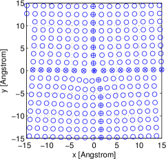
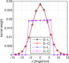
(a) (b) (c)

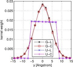
Figure 1: (a) The arrangement of the atoms in an edge dislocation gives a rather regular sample distribution. Lines of atoms in both x- ($\otimes$) and y-direction ($\oplus$) are selected. A Gaussian (G) and a uniform (U) kernel function for LCR (C) and LLR (L) are directly placed above the crossing atom of these two lines. This atom is the centre of the shown coordinate system. Horizontal (b) and vertical (c) slices of the kernel functions are given for the selected atoms.

To ascertain the effect of local constant regression ($P=0$ in Equation 8) and local linear regression ($P=1$ in Equation 8) on our atomistic dataset we compute the difference between the kernel weights arising from both regression models. For ease of exposition we select a Gaussian (with a standard deviation of $4.31\mathrm{\AA}$) and a uniform kernel (with a bandwidth of $7.50\mathrm{\AA}$ to adjust for the different shape of the kernel) Marron88 for smoothing. The kernels are placed over a selected atom as shown in Figure 1 and the associated weights are computed (slices of the kernel weights are plotted in Figure 1). As can be observed, the kernel weights arising from both regression models are effectively identical. The reason for this is due to the almost uniform spacing of the atoms which has the effect of rendering the off diagonal blocks in ${\bf B}^{T}{\bf W}{\bf B}$ of Equation 8 with values very close to zero in the LLR model. Therefore, the kernels for $P=0$ and $P=1$ are practically identical (see (Takeda07, , Section II.D) for a discussion).

We take the definition of virial stress from Equation 1 and replace the uniform kernel with the LLR equivalent kernel according to Equation 8 and set ${\bm{\sigma}}_{i}\rightarrow{\bm{\sigma}}_{i}/V_{i}$. With respect to the analytical solution of anisotropic linear elasticity Hirth82 (elastic constants taken from Lazarus49 ), the LLR model obtains a $0.126$ percent increase in root mean squared error (RMSE) as compared to the LCR model of virial stress. This difference is negligible and indicates that there is no substantial difference between the predicted stress arising from models. Replacing the uniform kernel with a Gaussian kernel, thereby yielding an altered virial stress, results in a similar observation: the difference between the output of both models is barely perceptible (relative increase in RMSE: $0.056$ percent).

4.2 Infinite plate with circular notch

In our second simulation we consider the problem of an infinite plate with a circular notch subject to uniaxial loading. The base system is altered by firstly removing a hole of radius $60a$ from the centre following by the application of a uniform tensile traction of $p=1\mathrm{GPa}$ on the edges normal to the $y$-direction. The equilibrium state is found at a temperature of zero Kelvin by energy minimization with relative tolerance $10^{-15}$. An atomistic solution to this problem was previously given in Admal10 ; Ulz13 , while an analytical solution of elasticity theory for the case of plane strain was provided in Lekhnitskii63 . However, the effect of surface free energy is neglected in the latter as it is considered to be small compared to the bulk energy in continuum mechanics. In Section 4.1, based on a direct comparison of kernel weights, we found that local linear regression (LLR) is effectively identical to local constant regression (LCR) when applied to an atomistic system that conforms to a regular grid. In this experiment we compare both models in the situation where we have a pore in the material. This pore introduces a boundary in the system only one side of which contains atoms.

We construct the simulation as follows: a circular slice with thickness $a$ centred at $x=60a$ and $y=0\mathrm{\AA}$ is taken as our atomistic dataset. The slice has radius $30a$ giving 6,329 data points (Figure 2). We fit both the LCR and LLR models to this dataset. The assigned weights for both LCR and LLR are shown in Figure 2 for a uniform and a Gaussian kernel (as described in Section 4.1). If we take the Gaussian kernel as our example, we can immediately observe the effect of the data-adaptive equivalent kernel at the boundary of the material (Figure 2(b)). As there are no atoms in the negative x-direction the kernels are therefore truncated in their extent in this region. The red line with circular markers denotes the Gaussian kernel weights in the LCR model, while the black line with asterisk-style markers denotes the equivalent kernel in the LLR model. It is clear that the equivalent kernel has adapted to the local density of the data at the boundary: versus the LCR Gaussian kernel, the equivalent kernel distributes substantially more weight to the cluster of atoms lying on or very close to the boundary ($\leq 2.5\mathrm{\AA}$), while considerably downweighting those atoms located further away ($>2.5\mathrm{\AA}$). The equivalent kernel therefore compensates for the lack of atoms in the negative x-direction by up-weighting the contribution of the boundary atoms to the estimation of the average stress at the boundary. As the stress at the boundary atoms is substantially different to that in the interior, this adaptation is beneficial for prediction of stress at the boundary - this estimate will be dominated by the stress of boundary atoms, with very little contribution from more distant atoms. The net result of this kernel adaptation is a better fit to the atomistic data in the boundary region.

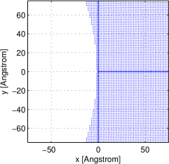
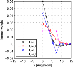
(a) (b) (c)

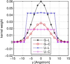
Figure 2: (a) The arrangement of the atoms at the notch. Lines of atoms in both x- ($+$) and y-direction ($\times$) are selected. A Gaussian (G) and a uniform (U) kernel function for LCR (C) and LLR (L) are directly placed above the crossing atom of these two lines. This atom is the centre of the shown coordinate system. Horizontal (b) and vertical (c) slices of the kernel functions are given for the selected atoms.

Unfortunately, despite our expectations to the contrary, the improved fit at the boundary does not translate into an improved estimate of virial stress as given by Equation 1. The central cause of this are surface effects which have an impact on the atomistic stress per atom values ${{\bm{\sigma}}}_{i}$ given in Equation 1. More specifically, the surface effects cause the stress per atom value of the boundary atoms to be very different from the stress per atom values of those atoms only a few $\mathrm{\AA}$ into the material from the boundary. This can be seen by observing the patterns of the stress per atom values (indicated by the diamond symbol) from $0\mathrm{\AA}$ to $10\mathrm{\AA}$ in Figure 3(b). Due to the large discontinuity in stress over a small distance in this region, the improved fit of the LLR model at the boundary translates into a much poorer fit in the region several units of $\mathrm{\AA}$ into the material. The LLR model effectively attempts to smooth out this discontinuity, resulting in a poor fit in the locality of the discontinuity. Ideally the impact of the surface-affected atoms should be restricted to the surface itself, necessitating that the kernel assign negligible weight to such atoms when computing the stress at points in the interior. However the equivalent kernel, due to its data-adaptive capability, assigns a much higher weight to boundary atoms than the LCR kernel, when computing the average stress for atoms in the region adjacent to the boundary ($0\mathrm{\AA}$ to $10\mathrm{\AA}$ in Figure 3(b)). In contrast, the weights assigned to the surface atoms by the LCR kernel do not differ substantially to the weights assigned by that kernel to atoms in the interior, effectively curtailing the impact of surface effects on the predicted average stress of interior atoms. The net result is that the classical virial stress (that is, the LCR model), due to its poor fit at the boundary, actually yields a superior overall fit to the atomistic data due to its insensitivity to the stress discontinuity near the surface. This observation negates any potential benefit brought about through modelling the dataset, and in particular, the boundary region, using LLR.

(a)
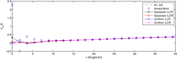
(b)

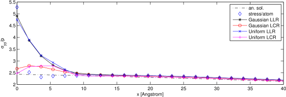
Figure 3: Stress distribution for notch problem. Normalized normal stresses (a) $\sigma_{xx}$ and (b) $\sigma_{yy}$ in positive $x$-direction starting at the radius of the notch and at $y=$0Å. The analytical solution (surface effects disregarded) is given by the dotdashed line, the volume-related stress per atom values (${\bm{\sigma}}_{i}/V_{i}$) are given by ($\Diamond$).

5 Discussion and conclusion

The objective of this paper was to investigate the applicability of automatic kernel carpentry for the purposes of modelling atomistic stress using non-parametric kernel regression. In many materials of interest, flaws or boundaries result in an asymmetry in the distribution of atoms. Automatic kernel carpentry provides a principled means of adapting the weighting of the kernel according to the local density of the data samples. It is well known that the local linear regression (LLR) model yields a reduction in the bias of the regression function, with a modest increase in variance, yielding, in many cases, an overall improved fit to the data. This data-adapted kernel is known as the equivalent kernel in the statistical literature. In this work we replaced the uniform kernel in the virial stress by the equivalent kernel formed by a LLR model yielding an altered virial stress. The predictive accuracy of our LLR model was then compared to the local constant regression (LCR) model of UlzMoran13 . The key finding of our experimental validation is that automatic kernel carpentry, as given by fitting an LLR model to atomistic stress, does not yield an increase in the accuracy of the virial stress estimate versus the LCR model of UlzMoran13 . The main barriers to effective application of the LLR model proved to be both the highly regular arrangement of atoms in the crystalline solids under study and the surface-affected atoms at the boundary of the materials.

Firstly, the regular spacing of the atoms in crystalline solids resulted in the LLR equivalent kernel to be effectively identical to that obtained using the LCR model in the interior. If the atoms are placed in a perfect lattice there is no asymmetry in the distribution of the atoms, and therefore no scope for kernel adaptation as all points in the space have equivalent density. The net effect of this is that the LCR model provides similar stress estimates to the LLR model, at a fraction of the computational cost. Secondly surface effects, which cause the stress of surface atoms to vary greatly from adjacent atoms located in the inner regions of the material, negated any benefit arising from the boundary bias correcting capability of the LLR model. There is effectively a discontinuity in the stress distribution in the region near and at the surface, which contradicts the basic smoothness assumption of non-parametric kernel regression. In our experimental validation we observed that the LCR model is less effected by this discontinuity than the LLR model. The influence of the highly surface-affected atoms at the boundary onto the averaged stress in the proximity of the boundary is undesirably magnified by the weight distribution of the equivalent kernel, that is, substantially more weight is assigned to surface atoms versus those atoms in the interior of the material. In contrast, the averaged stress given by the LCR model in the proximity of the surface is much less influenced by surface effects. We identified the cause of this to be the more equal weighting applied by the LCR kernel to atoms in the interior and to those at the surface, thereby providing an average that is less sensitive to discontinuities in the atomistic data. In other words, the LCR model, due to its increased bias at boundary regions, essentially restricts the contribution of surface atoms on the average stress prediction at points in the interior. A local linear regression model with change points SanchezBorrego06 would be a possible means of handling these discontinuities in the atomistic data - we leave this investigation to future work. Given these observations we found that the additional computational effort of implementing the LLR model versus the LCR model is not justified for the modelling of atomistic stress in crystalline solids.

Nevertheless, despite demonstrating that LLR is ineffective for the example of crystalline solids, our study has highlighted two useful criteria that can be applied by the research community for evaluating when best to apply LLR versus LCR. Firstly, if the material under study has a highly irregular distribution of atoms in the interior, then LLR is very likely to offer a much better fit to the data, and therefore provide more accurate predictions for the physical quantity of interest. Secondly, LLR is also likely to give more accurate predictions in the situation where the material under study is not characterised by wide variations (discontinuities) in the predictive variable (in the example of this paper, stress) over small changes in the covariate (in this paper, distance). Given these criteria, we believe LLR may be beneficial for similar problems in fluid dynamics and solids with highly irregular structure (for example, amorphous solids). In addition, the LLR framework may also be useful for modelling interfacial regions between two bulk phases (considered as a two-dimensional continuum) and the transition region near the line of contact of three media (considered as a one-dimensional continuum).

References

- (1) Admal, N.C., Tadmor, E.B.: A unified interpretation of stress in molecular systems. J. Elasticity 100, 63–143 (2010)
- (2) Cheung, K.S., Yip, S.: Atomic-level stress in an inhomogeneous system. J. Appl. Phys. 70, 5688–5690 (1991)
- (3) Clausius, R.J.E.: On a mechanical theorem applicable to heat. Phil. Mag. 40, 122–7 (1870)
- (4) Curtin, W.A., Miller, R.E.: Atomistic/continuum coupling in computational materials science. Modelling Simul. Mater. Sci. Eng. 11, R33 (2003)
- (5) Fan, J., Gijbels, I.: Local polynomial modelling and its applications. (London: Chapman & Hall) (1996)
- (6) Hardy, R.J.: Formulas for determining local properties in molecular‐dynamics simulations: shock waves. J. Chem. Phys. 76, 622–628 (1982)
- (7) Hastie, T., Tibshirani, R., Friedman, J.: The Elements of Statistical Learning: Data Mining, Inference, and Prediction. (New York: Springer) (2009)
- (8) Hirth, J.P., Lothe, J.: Theory of Dislocations, 2 edn. (New York: John Wiley & Sons Inc) (1982)
- (9) Irving, J.H., Kirkwood, J.G.: The statistical mechanical theory of transport processes. IV. the equations of hydrodynamics. J. Chem. Phys. 18, 817–829 (1950)
- (10) Kay, S.: Fundamentals of Statistical Signal Processing, Volume I: Estimation Theory. (New Jersey: Prentice Hall) (1993)
- (11) LAMMPS: http://lammps.sandia.gov
- (12) Lazarus, D.: The variation of the adiabatic elastic constants of KCl, NaCl, CuZn, Cu, and Al with pressure to 10,000 bars. Phys. Rev. 76, 545–553 (1949)
- (13) Lekhnitskii, S.G.: Theory of elasticity of an anisotropic elastic body. (San Francisco: Holden-Day, Inc.) (1963). Originally published as: 1950 Teoriia Uprugosti Anisotropnovo Tela (Moscow and Leningrad: Government Publishing House for Technical-Theoretical Works)
- (14) Marron, J.S., Nolan, D.: Canonical kernels for density estimation. Stat. Probab. Lett. 7, 195–199 (1988)
- (15) Maxwell, J.C.: On reciprocal figures, frames and diagrams of forces. Trans. R. Soc. Edinburgh XXVI, 1–43 (1870)
- (16) Maxwell, J.C.: Van der Waals on the continuity of the gaseous and liquid states. Nature 10, 477–480 (1874)
- (17) Miller, R.E., Tadmor, E.B.: A unified framework and performance benchmark of fourteen multiscale atomistic/continuum coupling methods. Modelling Simul. Mater. Sci. Eng. 17, 053001 (2009)
- (18) Murdoch, A.I.: The motivation of continuum concepts and relations from discrete considerations. Q. J. Mechanics Appl. Math. 36, 163–187 (1983)
- (19) Murdoch, A.I.: A critique of atomistic definitions of the stress tensor. J. Elasticity 88, 113–140 (2007)
- (20) Murdoch, A.I.: Physical Foundations of Continuum Mechanics. (Cambridge: Cambridge University Press) (2012)
- (21) Murdoch, A.I., Bedeaux, D.: Continuum equations of balance via weighted averages of microscopic quantities. Proc. R. Soc. Lond. Math. Phys. Sci. 445, 157–179 (1994)
- (22) Noll, W.: Die Herleitung der Grundgleichungen der Thermomechanik der Kontinua aus der Statistischen Mechanik. Indiana Univ. Math. J. (formerly: J. Ration. Mech. Anal.) 4, 627–646 (1955)
- (23) Sánchez-Borrego, I.R., Martínez-Miranda, M.D., González-Carmona, A.: Local linear kernel estimation of the discontinuous regression function. Comput. Stat. 21, 557–569 (2006)
- (24) Sun, Z.H., Wang, X.X., Soh, A.K., Wu, H.A.: On stress calculations in atomistic simulations. Modelling Simul. Mater. Sci. Eng. 14, 423–431 (2006)
- (25) Takeda, H., Farsiu, S., Milanfar, P.: Kernel regression for image processing and reconstruction. IEEE Trans. Image Process. 16, 349–366 (2007)
- (26) Ulz, M.H., Mandadapu, K.K., Papadopoulos, P.: On the estimation of spatial averaging volume for determining stress using atomistic methods. Modelling Simul. Mater. Sci. Eng. 21, 015,010 (2013)
- (27) Ulz, M.H., Moran, S.J.: A Gaussian mixture modelling approach to the data-driven estimation of atomistic support for continuum stress. Modelling Simul. Mater. Sci. Eng. 20, 065,009 (2012)
- (28) Ulz, M.H., Moran, S.J.: Optimal kernel shape and bandwidth for atomistic support of continuum stress. Modelling Simul. Mater. Sci. Eng. 21, 085,017 (2013)
- (29) WebbIII, E.B., Zimmerman, J.A., Seel, S.C.: Reconsideration of continuum thermomechanical quantities in atomic scale simulations. Math. Mech. Solids 13, 221–266 (2008)
- (30) Zeng, X., Li, S.: Recent developments on concurrent multiscale simulations. In: Advances in Engineering Mechanics, Volume 1 (eds. Q.H. Qin and B. Sun). (Nova Science Publishers, Inc.) (2010)
- (31) Zhou, X.W., Wadley, H.N.G., Johnson, R.A., Larson, D.J., Tabat, N., Cerezo, A., Petford-Long, A.K., Smith, G.D.W., Clifton, P.H., Martens, R.L., Kelly, T.F.: Atomic scale structure of sputtered metal multilayers. Acta Mater. 49, 4005–4015 (2001)
- (32) Zimmerman, J.A., WebbIII, E.B., Hoyt, J.J., Jones, R.E., Klein, P.A., Bammann, D.J.: Calculation of stress in atomistic simulation. Modelling Simul. Mater. Sci. Eng. 12, S319–332 (2004)