Wiggins: Detecting Valuable Information
in Dynamic Networks Using Limited Resources

Abstract

Detecting new information and events in a dynamic network by probing individual nodes has many practical applications: discovering new webpages, analyzing influence properties in network, and detecting failure propagation in electronic circuits or infections in public drinkable water systems. In practice, it is infeasible for anyone but the owner of the network (if existent) to monitor all nodes at all times. In this work we study the constrained setting when the observer can only probe a small set of nodes at each time step to check whether new pieces of information (items) have reached those nodes.

We formally define the problem through an infinite time generating process that places new items in subsets of nodes according to an unknown probability distribution. Items have an exponentially decaying novelty, modeling their decreasing value. The observer uses a probing schedule (i.e., a probability distribution over the set of nodes) to choose, at each time step, a small set of nodes to check for new items. The goal is to compute a schedule that minimizes the average novelty of undetected items. We present an algorithm, wiggins, to compute the optimal schedule through convex optimization, and then show how it can be adapted when the parameters of the problem must be learned or change over time. We also present a scalable variant of wiggins for the MapReduce framework. The results of our experimental evaluation on real social networks demonstrate the practicality of our approach.

“Have you found it, Wiggins?”

[Sherlock Holmes in A Study in Scarlet]

1 Introduction

Many applications require the detection of events in a network as soon as they happen or shortly thereafter, as the value of the information obtained by detecting the events decays rapidly as time passes. For example, an emerging trend in algorithmic stock trading is the use of automatic search through the Web and social networks for pieces of information that can be used in trading decisions before they appear in the more popular news sites [10, 23, 14, 26]. Similarly, intelligence, business and politics analysts are scanning online sources for new information or rumors. While new items are often reblogged, retweeted, and posted on a number of sites, it is sufficient to find an item once, as fast as possible, before it loses its relevance or freshness. There is no benefit in seeing multiple copies of the same news item or rumor. This is also the case when monitoring for intrusions, infections, or defects in, respectively, a computer network, a public water system, or a large electronic circuit.

Monitoring for new events or information is a fundamental search and detection problem in a distributed data setting, not limited to social networks or graph analysis. In this setting, the data is distributed among a large number of nodes, and new items appear in individual nodes (for example, as the products of processing the data available locally at the node), and may propagate (being copied) to neighboring nodes on a physical or a virtual network. The goal is to detect at least one copy of each new item as soon as possible. The search application can access any node in the system, but it can only probe (i.e., check for new items on) a few nodes at a time. To minimize the time to find new items, the search application needs to optimize the schedule of probing nodes, taking into account (i) the distribution of copies of items among the nodes (to choose which nodes to probe), and (ii) the decay of the items’ novelty (or relevance/freshness) over time (to focus the search on most relevant items). The main challenge is how to devise a good probing schedule in the absence of prior knowledge about the generation and distribution of items in the network.

Contributions

In this work we study the novel problem of computing an optimal node probing schedule for detecting new items in a network under resource scarceness, i.e., when only a few nodes can be probed at a time. Our contributions to the study of this problem are the following:

We formalize a generic process that describes the creation and distribution of information in a network, and define the computational task of learning this process by probing the nodes in the network according to a schedule. The process and task are parametrized by the resource limitations of the observer and the decay rate of the novelty of items. We introduce a cost measure to compare different schedules: the cost of a schedule is the limit of the average expected novelty of uncaught items at each time step. On the basis of these concepts, we formally define the Optimal Probing Schedule Problem, which requires to find the schedule with minimum cost.

We conduct a theoretical study of the cost of a schedule, showing that it can be computed explicitly and that it is a convex function over the space of schedules. We then introduce wiggins, an algorithm to compute the optimal schedule by solving a constrained convex optimization problem through the use of an iterative method based on Lagrange multipliers.

We discuss variants of wiggins for the realistic situation where the parameters of the process needs to be learned or can change over time. We show how to compute a schedule which is (probabilistically) guaranteed to have a cost very close to the optimal by only observing the generating process for a limited amount of time. We also present a MapReduce adaptation of wiggins to handle very large networks.

Finally, we conduct an extensive experimental evaluation of wiggins and its variants, comparing the performances of the schedules it computes with natural baselines, and showing how it performs extremely well in practice on real social networks when using well-established models for generating new items (e.g., the independence cascade model [17]).

To the best of our knowledge, the problem we study is novel and we are the first to devise an algorithm to compute an optimal schedule, both when the generating process parameters are known and when they need to be learned.

Paper Organization. In Sect. 2 we give introductory definitions, and formally introduce the settings and the problem. We discuss related works in Sect. 3. In Sect. 4 we describe our algorithm wiggins and its variants. The results of our experimental evaluation are presented in Sect. 5. We conclude by outlining directions for future work in Sect. 6.

2 Problem Definition

In this section we formally introduce the problem and define our goal.

Let $G=(V,E)$ be a graph with $|V|=n$ nodes. W.l.o.g. we let $V=[n]$. Let $\mathcal{F}\subseteq 2^{V}$ be a collection of subsets of $V$, i.e., a collection of sets of nodes. Let $\pi$ be a function from $\mathcal{F}$ to $[0,1]$ (not necessarily a probability distribution). We model the generation and diffusion of information in the network by defining a generating process $\Gamma=(\mathcal{F},\pi)$. $\Gamma$ is a infinite discrete-time process which, at each time step $t$, generates a collection of sets $\mathcal{I}_{t}\subseteq\mathcal{F}$ such that each set $S\in\mathcal{F}$ is included in $\mathcal{I}_{t}$ with probability $\pi(S)$, independently of $t$ and of other sets generated at time $t$ and at time $t^{\prime}<t$. For any $t$ and any $S\in\mathcal{I}_{t}$, the ordered pair $(t,S)$ represents an item - a piece of information that was generated at time $t$ and reached instantaneously the nodes in $S$. We choose to model the diffusion process as instantaneous because this abstraction accurately models the view of an outside resource-limited observer that does not have the resources to monitor simultaneously all the nodes in the network at the fine time granularity needed to observe the different stages of the diffusion process.

Probing and schedule. The observer can only monitor the network by probing nodes. Formally, by probing a node $v\in V$ at time $t$, we mean obtaining the set $I(t,v)$ of items $(t^{\prime},S)$ such that $t^{\prime}\leq t$ and $v\in S$:

$$I(t,v)\coloneqq\{(t^{\prime},S)~{}:~{}t^{\prime}\leq t,S\in\mathcal{I}_{t^{\prime}},v\in S\}\enspace.$$

Let $U_{t}$ be the union of the sets $\mathcal{I}_{t^{\prime}}$ generated by $\Gamma$ at any time $t^{\prime}\leq t$, and so $I(t,v)\subseteq U_{t}$.

We model the resource limitedness of the observer through a constant, user-specified, parameter $c\in\mathbb{N}$, representing the maximum number of nodes that can be probed at any time, where probing a node $v$ returns the value $I(t,v)$.

The observer chooses the $c$ nodes to probe by following a schedule. In this work we focus on memoryless schedules, i.e., the choice of nodes to probe at time $t$ is independent from the choice of nodes probed at any time $t^{\prime}<t$. More precisely, a probing $c$-schedule $\mathsf{p}$ is a probability distribution on $V$. At each time $t$, the observer chooses a set $P_{t}$ of $c$ nodes to probe, such that $P_{t}$ is obtained through random sampling of $V$ without replacement according to $\mathsf{p}$, independently from $P_{t^{\prime}}$ from $t^{\prime}<t$.

Caught items, uncaught items, and novelty. We say that an item $(t^{\prime},S)$ is caught at time $t\geq t^{\prime}$ iff

a node $v\in S$ is probed at time $t$; and

no node in $S$ was probed in the interval $[t^{\prime},t-1]$.

Let $C_{t}$ be the set of items caught by the observer at any time $t^{\prime}\leq t$. We have $C_{t}\subseteq U_{t}$. Let $N_{t}=U_{t}\setminus C_{t}$ be the set of uncaught items at time $t$, i.e., items that were generated at any time $t^{\prime}\leq t$ and have not been caught yet at time $t$. For any item $(t^{\prime},S)\in N_{t}$, we define the $\theta$-novelty of $(t^{\prime},S)$ at time $t$ as

$$\mathsf{f}_{\theta}(t,t^{\prime},S)\coloneqq\theta^{t-t^{\prime}},$$

where $\theta\in(0,1)$ is a user-specified parameter modeling how fast the value of an item decreases with time if uncaught. Intuitively, pieces of information (e.g., rumors) have high value if caught almost as soon as they have appeared in the network, but their value decreases fast (i.e., exponentially) as more time passes before being caught, to the point of having no value in the limit.

Load of the system and cost of a schedule. The set $N_{t}$ of uncaught items at time $t$ imposes a $\theta$-load, $L_{\theta}(t)$, on the graph at time $t$, defined as the sum of the $\theta$-novelty at time $t$ of the items in $N_{t}$:

$$L_{\theta}(t)\coloneqq\sum_{(t^{\prime},S)\in N_{t}}\mathsf{f}_{\theta}(t,t^{\prime},S)\enspace.$$

The quantity $L_{\theta}(t)$ is a random variable, depending both on $\Gamma$ and on the probing schedule $\mathsf{p}$, and as such it has an expectation $\mathbb{E}[L_{\theta}(t)]$ w.r.t. all the randomness in the system. The $\theta$-cost of a schedule $\mathsf{p}$ is defined as the limit, for $t\rightarrow\infty$, of the average expected load of the system:

$$\mathsf{cost}_{\theta}(\mathsf{p}) \coloneqq\lim_{t\rightarrow\infty}\frac{1}{t}\sum_{t^{\prime}\leq t}\mathbb{E}[L_{\theta}(t)]$$

$$=\lim_{t\rightarrow\infty}\frac{1}{t}\sum_{t^{\prime}\leq t}\mathbb{E}\left[\sum_{(t^{\prime\prime},S)\in N_{t^{\prime}}}\mathsf{f}_{\theta}(t^{\prime},t^{\prime\prime},S)\right]\enspace.$$

Intuitively, the load at each time indicates the amount of novelty we did not catch at that time, and the cost function measures the average of such loss over time. The limit above always exists (Lemma 1).

We now have all the necessary ingredients to formally define the problem of interest in this work.

Problem definition. Let $G=(V,E)$ be a graph and $\Gamma=(\mathcal{F},\pi)$ be a generating process on $G$. Let $c\in\mathbb{N}$ and $\theta\in(0,1)$. The $(\theta,c)$-Optimal Probing Schedule Problem ($(\theta,c)$-OPSP) requires to find the optimal $c$-schedule $\mathsf{p}^{*}$, i.e., the schedule with minimum $\theta$-cost over the set $\mathsf{S}_{c}$ of $c$-schedules:

$$\mathsf{p}^{*}=\arg\min_{\mathsf{p}}\{\mathsf{cost}_{\theta}(\mathsf{p}),\mathsf{p}\in\mathsf{S}_{c}\}\enspace.$$

Thus, the goal is to design a $c$-schedule that discovers the maximum number of items weighted by their novelty value (which correspond to those generated most recently). The parameter $\theta$ controls how fast the novelty of an item decays, and influences the choices of a schedule. When $\theta$ is closed to $0$, items are relevant only for a few steps and the schedule must focus on the most recently generated items, catching them as soon as they are generated (or at most shortly thereafter). At the other extreme ($\theta\approx 1$), an optimal schedule must maximizes the total number of discovered items, as their novelty decays very slowly.

Viewing the items as “information” disseminated in the network, an ideal schedule assigns higher probing probability to nodes that act as information hubs, i.e., nodes that receive a large number of items. Thus, an optimal schedule $\mathsf{p}^{*}$, identifies information hubs among the nodes. This task (finding information hubs) can be seen as the complement of the influence maximization problem [17, 18]. In the influence maximization problem we look for a set of nodes that generate information that reach most nodes. In the information hubs problem, we are interested in a set of nodes that receive the most of information, thus the most informative nodes for an observer.

In the following sections, we may drop the specification of the parameters from $\theta$-novelty, $\theta$-cost, $\theta$-load, and $c$-schedule, and from their respective notation, as the parameters will be clear from the context.

3 Related Work

The novel problem we focus on in this work generalizes and complements a number of problems studied in the literature.

The “Battle of Water Sensor Network” challenge [29] motivated a number of works on outbreak detection: the goal is to optimally place static or moving sensors in water networks to detect contamination [24, 20, 13]. The optimization can be done w.r.t. a number of objectives, such as maximizing the probability of detection, minimizing the detection time, or minimizing the size of the subnetwork affected by the phenomena [24]. A related work [1] considered sensors that are sent along fixed paths in the network with the goal of gathering sufficient information to locate possible contaminations. Early detection of contagious outbreaks by monitoring the neighborhood (friends) of a randomly chosen node (individual) was studied by Christakis and Fowler [7]. Krause et al. [21] present efficient schedules for minimizing energy consumption in battery operated sensors, while other works analyzed distributed solutions with limited communication capacities and costs [22, 11, 19]. In contrast, our work is geared to detection in huge but virtual networks such as the Web or social networks embedded in the Internet, where it is possible to “sense” or probe (almost) any node at approximately the same cost. Still only a restricted number of nodes can be probed at each steps but the optimization of the probing sequence is over a much larger domain, and the goal is to identify the outbreaks (items) regardless of their size and solely by considering their interest value.

Our methods complement the work on Emerging Topic Detection where the goal is to identify emergent topics in a social network, assuming full access to the stream of all postings. Providers, such as Twitter or Facebook, have an immediate access to all tweets or postings as they are submitted to their server [4, 25]. Outside observers need an efficient mechanism to monitor changes, such as the methods developed in this work.

Web-crawling is another research area that study how to obtain the most recent snapshots of the web. However, it differs from our model in two key points: our model allows items to propagate their copies, and they will be caught if any of their copies is discovered (where snapshots of a webpage belong to that page only), and all the generated items should be discovered (and not just the recent ones) [8, 32].

The goal of News and Feed Aggregation problem is to capture updates in news websites (e.g. by RSS feeds) [28, 15, 3, 30]. Our model differs from that setting in that we consider copies of the same news in different web sites as equivalent and therefore are only interested in discovering one of the copies.

4 The WIGGINS Algorithm

In this section we present the algorithm wiggins (and its variants) for solving the Optimal Probing Schedule Problem $(\theta,c)$-OPSP for generating process $\Gamma=(\mathcal{F},\pi)$ on a graph $G=(V,E)$.

We start by assuming that we have complete knowledge of $\Gamma$, i.e., we know $\mathcal{F}$ and $\pi$. This strong assumption allows us to study the theoretical properties of the cost function and motivates the design of our algorithm, wiggins, to compute an optimal schedule. We then remove the assumption and show how we can extend wiggins to only use a collection of observations from $\Gamma$. Then we discuss how to recalibrate our algorithms when the parameters of the process (e.g., $\pi$ or $\mathcal{F}$) change over time. Finally, we show an algorithm for the MapReduce framework that allows us to scale to large networks.

4.1 Computing the Optimal Schedule

We first conduct a theoretical analysis of the cost function $\mathsf{cost}_{\theta}$.

Analysis of the cost function

Assume for now that we know $\Gamma$, i.e., we have complete knowledge of $\mathcal{F}$ and $\pi$. Under this assumption, we can exactly compute the $\theta$-cost of a $c$-schedule.

Lemma 1.

Let $\mathsf{p}=(\mathsf{p}_{1},\ldots,\mathsf{p}_{n})$ be a $c$-schedule. Then

$$\mathsf{cost}(\mathsf{p})\coloneqq\lim_{t\rightarrow\infty}\frac{1}{t}\sum_{t^{\prime}=0}^{t}\mathbb{E}[L_{\theta}(t^{\prime})]=\sum_{S\in\mathcal{F}}\frac{\pi(S)}{1-\theta(1-\mathsf{p}(S))^{c}},$$ (1)

where $\mathsf{p}(S)=\sum_{v\in S}\mathsf{p}_{v}$.

Proof.

Let $t$ be a time step, and consider the quantity $\mathbb{E}[L_{\theta}(t)]$. By definition we have

$$\mathbb{E}[L_{\theta}(t)]=\mathbb{E}\left[\sum_{(t^{\prime},S)\in N_{t}}\mathsf{f}_{\theta}(t,t^{\prime},S)\right]=\mathbb{E}\left[\sum_{(t^{\prime},S)\in N_{t}}\theta^{t-t^{\prime}}\right],$$

where $N_{t}$ is the set of uncaught items at time $t$. Let now, for any $t^{\prime}\leq t$, $N_{t,t^{\prime}}\subseteq N_{t}$ be the set of uncaught items in the form $(t^{\prime},S)$. Then we can write

$$\mathbb{E}[L_{\theta}(t)]=\mathbb{E}\left[\sum_{t^{\prime}=0}^{t}\sum_{(t^{\prime},S)\in N_{t,t^{\prime}}}\theta^{t-t^{\prime}}\right]\enspace.$$

Define now, for each $S\in\mathcal{F}$, the random variable $X_{S,t^{\prime},t}$ which takes the value $\theta^{t-t^{\prime}}$ if $(t^{\prime},S)\in N_{t,t^{\prime}}$, and $0$ otherwise. Using the linearity of expectation, we can write:

$$\mathbb{E}[L_{\theta}(t)] =\sum_{S\in\mathcal{F}}\sum_{t^{\prime}=0}^{t}\mathbb{E}[X_{S},t^{\prime},t]$$

$$=\sum_{S\in\mathcal{F}}\sum_{t^{\prime}=0}^{t}\theta^{t-t^{\prime}}\Pr(X_{S,t,t^{\prime}}=\theta^{t-t^{\prime}})\enspace.$$ (2)

The r.v. $X_{S,t,t^{\prime}}$ takes value $\theta^{t-t^{\prime}}$ if and only if the following two events $E_{1}$ and $E_{2}$ both take place:

$E_{1}$: the set $S\in F$ belongs to $\mathcal{I}_{t^{\prime}}$, i.e., is generated by $\Gamma$ at time $t^{\prime}$;

$E_{2}$: the item $(t^{\prime},S)$ is uncaught at time $t$. This is equivalent to say that no node $v\in S$ was probed in the time interval $[t^{\prime},t]$. We have $\Pr(E_{1})=\pi(S)$, and

$$\Pr(E_{2})=(1-\mathsf{p}(S))^{c(t-t^{\prime})}\enspace.$$

The events $E_{1}$ and $E_{2}$ are independent, as the process of probing the nodes is independent from the process of generating items, therefore, we have

$$\Pr(X_{S,t,t^{\prime}}=\theta^{t-t^{\prime}})=\Pr(E_{1})\Pr(E_{2})=\pi(S)(1-\mathsf{p}(S))^{c(t-t^{\prime})}\enspace.$$

We can plug this quantity in the rightmost term of (4.1) and write

$$\lim_{t\rightarrow\infty}\mathbb{E}[L_{\theta}(t)] =\lim_{t\rightarrow\infty}\sum_{S\in\mathcal{F}}\sum_{t^{\prime}=0}^{t}\theta^{t-t^{\prime}}\pi(S)(1-\mathsf{p}(S))^{c(t-t^{\prime})}$$

$$=\lim_{t\rightarrow\infty}\sum_{S\in\mathcal{F}}\pi(S)\sum_{t^{\prime}=0}^{t}(\theta(1-\mathsf{p}(S))^{c})^{t}$$

$$=\sum_{S\in\mathcal{F}}\frac{\pi(S)}{1-\theta(1-\mathsf{p}(S))^{c}},$$ (3)

where we used the fact that $\theta(1-\mathsf{p}(S))^{c}<1$. We just showed that the sequence $(\mathbb{E}[L_{\theta}(t)])_{t\in\mathbb{N}}$ converges as $t\rightarrow\infty$. Therefore, its Cesàro mean, i.e., $\lim_{t\rightarrow\infty}\frac{1}{t}\sum_{t^{\prime}=0}^{t}\mathbb{E}[L_{\theta}(t)]$, equals to its limit [12, Sect. 5.4] and we have

$$\mathsf{cost}_{\theta}(\mathsf{p}) =\lim_{t\rightarrow\infty}\frac{1}{t}\sum_{t^{\prime}=0}^{t}\mathbb{E}[L_{\theta}(t)]=\lim_{t\rightarrow\infty}\mathbb{E}[L_{\theta}(t)]$$

$$=\sum_{S\in\mathcal{F}}\frac{\pi(S)}{1-\theta(1-\mathsf{p}(S))^{c}}\enspace.$$

∎

We now show that $\mathsf{cost}_{\theta}(\mathsf{p})$, as expressed by the r.h.s. of (1) is a convex function over its domain $\mathsf{S}_{c}$, the set of all possible $c$-schedules. We then use this result to show how to compute an optimal schedule.

Theorem 1.

The cost function $\mathsf{cost}_{\theta}(\mathsf{p})$ is a convex function over $\mathsf{S}_{c}$.

Proof.

For any $S\in\mathcal{F}$, let

$$f_{S}(\mathsf{p})=\frac{1}{1-\theta(1-\mathsf{p}(S))^{c}}\enspace.$$

The function $\mathsf{cost}_{\theta}(\mathsf{p})$ is a linear combination of $f_{S}(\mathsf{p})$’s with positive coefficients. Hence to show that $\mathsf{cost}_{\theta}(\mathsf{p})$ is convex it is sufficient to show that, for any $S\in\mathcal{F}$, $f_{S}(\mathsf{p})$ is convex.

We start by showing that $g_{S}(\mathsf{p})=\theta(1-\mathsf{p}(S))^{c}$ is convex. This is due to the fact that its Hessian matrix is positive semidefinite [2]:

$$\frac{\partial}{\partial\mathsf{p}_{i}\partial\mathsf{p}_{j}}g_{S}(\mathsf{p})=\left\{\begin{array}[]{lr}\theta c(c-1)(1-\mathsf{p}(S))^{c-2}&i,j\in S\\ 0&\text{otherwise}\end{array}\right.$$

Let $\mathbf{v}_{S}$ be a $n\times 1$ vector in $\mathbb{R}^{n}$ such that its $i$-th coordinate is $\left[c(c-1)(1-\mathsf{p}(S))^{c-2}\right]^{1/2}$ if $i\in S$, and $0$ otherwise. We can write the Hessian matrix of $g_{S}$ as

$$\nabla^{2}g_{S}=V_{S}*V_{S}^{\mathsf{T}},$$

and thus, $\nabla^{2}g_{S}$ is positive semidefinite matrix and $g$ is convex. From here, we have that $1-g_{S}$ is a concave function. Since $f_{S}(\mathsf{p})=\frac{1}{1-g_{S}(\mathsf{p})}$ and the function $h(x)=\frac{1}{x}$ is convex and non-increasing, then $f_{S}$ is a convex function. ∎

If for every $v\in V$, $S=\{v\}$ belongs to $\mathcal{F}$, then the function $g_{S}$ in the above proof is strictly convex, and so is $f_{S}$.

We then have the following corollary of Thm. 1.

Corollary 1.

Any schedule $\mathsf{p}$ with locally minimum cost is an optimal schedule (i.e., it has global minimum cost). Furthermore, if for every $v\in V$, $\{v\}$ belongs to $\mathcal{F}$, the optimal schedule is unique.

The algorithm

Corollary 1 implies that one can compute an optimal $c-$schedule $p^{*}$ (i.e., solve the $(\theta,c)$-OPSP) by solving the unconstrained minimization of $\mathsf{cost}_{\theta}$ over the set $\mathsf{S}_{c}$ of all $c$-schedules, or equivalently by solving the following constrained minimization problem on $\mathbb{R}^{n}$:

$$\boxed{\begin{array}[]{rrclcl}\displaystyle\min_{\mathsf{p}\in\mathbb{R}^{n}}&\lx@intercol\mathsf{cost}_{\theta}(\mathsf{p})\hfil\lx@intercol\\ &\displaystyle\sum_{i=1}^{n}\mathsf{p}_{i}&=&1\\ &\mathsf{p}_{i}&\geq&0&&\forall i\in\{1,\ldots,n\}\\ \end{array}}$$ (4)

Since the function $\mathsf{cost}_{\theta}$ is convex and the constraints are linear, the optimal solution can, theoretically, be found efficiently [2]. In practice though, available convex optimization problem solvers can not scale well with the number $n$ of variables, especially when $n$ is in the millions as is the case for modern graphs like online social networks or the Web. Hence we developed wiggins, an iterative method based on Lagrange multipliers [2, Sect. 5.1], which can scale efficiently and can be adapted to the MapReduce framework of computation [9], as we show in Sect. 4.4. While we can not prove that this iterative method always converges, we can prove (Thm. 2) that (i) if at any iteration the algorithm examines an optimal schedule, then it will reach convergence at the next iteration, and (ii) if it converges to a schedule, that schedule is optimal. In Sect. 5 we show our experimental results illustrating the convergence of wiggins in different cases.

wiggins takes as inputs the collection $\mathcal{F}$, the function $\pi$, and the parameters $c$ and $\theta$, and outputs a schedule $\mathsf{p}$ which, if convergence (defined in the following) has been reached, is the optimal schedule. It starts from a uniform schedule $\mathsf{p}^{(0)}$, i.e., $\mathsf{p}^{(0)}_{i}=1/n$ for all $1\leq i\leq n$, and iteratively refines it until convergence (or until a user-specified maximum number of iterations have been performed). At iteration $j\geq 1$, we compute, for each value $i$, $1\leq i\leq n$, the function

$$W_{i}(\mathsf{p}^{(j-1)})\coloneqq\sum_{\begin{subarray}{c}S\in\mathcal{F}\\ \mbox{\scriptsize{s.t. }}i\in S\end{subarray}}\frac{\theta c\pi(S)(1-\mathsf{p}^{(j-1)}(S))^{c-1}}{(1-\theta(1-\mathsf{p}^{(j-1)}(S))^{c})^{2}}$$ (5)

and then set

$$\mathsf{p}^{(j)}_{i}=\frac{\mathsf{p}^{(j-1)}_{i}W_{i}(\mathsf{p}^{(j-1)})}{\sum_{z=1}^{n}\mathsf{p}^{(j-1)}_{z}W_{z}(\mathsf{p}^{(j-1)})}\enspace.$$

The algorithm then checks whether $\mathsf{p}^{(j)}=\mathsf{p}^{(j-1)}$. If so, then we reached convergence and we can return $\mathsf{p}^{(j)}$ in output, otherwise we perform iteration $j+1$. The pseudocode for wiggins is in Algorithm 1. The following theorem shows the correctness of the algorithm in case of convergence.

Theorem 2.

We have that:

if at any iteration $j$ the schedule $\mathsf{p}^{(j)}$ is optimal, then wiggins reaches convergence at iteration $j+1$; and

if wiggins reaches convergence, then the returned schedule $\mathsf{p}$ is optimal.

Proof.

From the method of the Lagrange multipliers [2, Sect. 5.1], we have that, if a schedule $\mathsf{p}$ is optimal, then there exists a value $\lambda\in\mathbb{R}$ such that $\mathsf{p}$ and $\lambda$ form a solution to the following system of $n+1$ equations in $n+1$ unknowns:

$$\nabla[\mathsf{cost}_{\theta}(\mathsf{p})+\lambda(\mathsf{p}_{1}+\ldots+\mathsf{p}_{n}-1)]=0,$$ (6)

where the gradient on the l.h.s. is taken w.r.t. (the components of) $\mathsf{p}$ and to $\lambda$ (i.e., has $n+1$ components).

For $1\leq i\leq n$, the $i$-th equation induced by (6) is

$$\frac{\partial}{\partial\mathsf{p}_{i}}\mathsf{cost}_{\theta}(\mathsf{p})+\lambda=0,$$

or, equivalently,

$$\sum_{\begin{subarray}{c}S\in\mathcal{F}\\ \mbox{s.t.}i\in S\end{subarray}}\frac{\theta c\pi(S)(1-\mathsf{p}(S))^{c-1}}{(1-\theta(1-\mathsf{p}(S))^{c})^{2}}=\lambda\enspace.$$ (7)

The term on the l.h.s. is exactly $W_{i}(\mathsf{p})$. The $(n+1)$-th equation of the system (6) (i.e., the one involving the partial derivative w.r.t. $\lambda$) is

$$\sum_{z=1}^{n}\mathsf{p}_{z}=1\enspace.$$ (8)

Consider now the first claim of the theorem, and assume that we are at iteration $j$ such that $j$ is the minimum iteration index for which the schedule $\mathsf{p}^{(j)}$ computed at the end of iteration $j$ is optimal. Then, for any $i$, $1\leq i\leq n$, we have

$$W_{i}(\mathsf{p}^{(j)})=\lambda$$

because $\mathsf{p}^{(j)}$ is optimal and hence all identities in the form of (7) must be true. For the same reason, (8) must also hold for $\mathsf{p}^{(j)}$. Hence, for any $1\leq i\leq n$, we can write the value $\mathsf{p}^{(j+1)}_{i}$ computed at the end of iteration $j+1$ as

$$\mathsf{p}^{(j+1)}_{i}=\frac{\mathsf{p}^{(j)}_{i}W_{i}(\mathsf{p}^{(j)})}{\sum_{z=1}^{n}\mathsf{p}^{(j)}_{z}W_{z}(\mathsf{p}^{(j)})}=\frac{\mathsf{p}^{(j)}_{i}\lambda}{1\lambda}=\mathsf{p}^{(j)}_{i},$$

which means that we reached convergence and wiggins will return $\mathsf{p}^{(j+1)}$, which is optimal.

Consider the second claim of the theorem, and let $j$ be the first iteration for which $\mathsf{p}^{(j)}=\mathsf{p}^{(j-1)}$. Then we have, for any $1\leq i\leq n$,

$$\mathsf{p}^{(j)}_{i}=\frac{\mathsf{p}^{(j-1)}_{i}W_{i}(\mathsf{p}^{(j-1)})}{\sum_{z=1}^{n}\mathsf{p}^{(j-1)}_{z}W_{z}(\mathsf{p}^{(j-1)})}=\mathsf{p}^{(j-1)}_{i}\enspace.$$

This implies

$$W_{i}(\mathsf{p}^{(j-1)})=\sum_{z=1}^{n}\mathsf{p}^{(j-1)}_{z}W_{z}(\mathsf{p}^{(j-1)})$$ (9)

and the r.h.s. does not depend on $i$, and so neither does $W_{i}(\mathsf{p}^{(j-1)})$. Hence we have $W_{1}(\mathsf{p}^{(j-1)})=\dotsb=W_{n}(\mathsf{p}^{(j-1)})$ and can rewrite (9) as

$$W_{i}(\mathsf{p}^{(j-1)})=\sum_{z=1}^{n}\mathsf{p}^{(j-1)}_{z}W_{i}(\mathsf{p}^{(j-1)}),$$

which implies that the identity (8) holds for $\mathsf{p}^{(j-1)}$. Moreover, if we set

$$\lambda=W_{1}(\mathsf{p}^{(j-1)})$$

we have that all the identities in the form of (7) hold. Then, $\mathsf{p}^{(j-1)}$ and $\lambda$ form a solution to the system (6), which implies that $\mathsf{p}^{(j-1)}$ is optimal and so must be $\mathsf{p}^{(j)}$, the returned schedule, as it is equal to $\mathsf{p}^{(j-1)}$ because wiggins reached convergence. ∎

input : $\mathcal{F}$, $\pi$, $c$, $\theta$, and maximum number $T$ of iterations

output : A $c$-schedule $\mathsf{p}$ (with globally minimum $\theta$-cost, in case of convergence)

1 for $i\leftarrow 1$ to $n$ do

2       $\mathsf{p}_{i}\leftarrow 1/n$

3      

4 end for

5for $j\leftarrow 1$ to $T$ do

6       for $i\leftarrow 1$ to $n$ do

7             $W_{i}\leftarrow 0$

8            

9       end for

10      for $S\in\mathcal{F}$ do

11             for $i\in S$ do

12                   $W_{i}\leftarrow W_{i}+\frac{\theta c\pi(S)(1-\mathsf{p}(S))^{c-1}}{(1-\theta(1-\mathsf{p}(S))^{c})^{2}}$

13                  

14             end for

15            

16       end for

17      $\mathsf{p}_{\mathrm{old}}\leftarrow\mathsf{p}$

18       for $i\leftarrow 1$ to $n$ do

19             $\mathsf{p}_{i}\leftarrow\frac{\mathsf{p}_{i}W_{i}}{\sum_{i}\mathsf{p}_{i}W_{i}}$

20            

21       end for

22      if $\mathsf{p}_{\mathrm{old}}=\mathsf{p}$ then // test for convergence

23             break

24            

25       end if

26      

27 end for

28return $\mathsf{p}$

Algorithm 1 wiggins

4.2 Approximation through Sampling

We now remove the assumption, not realistic in practice, of knowing the generating process $\Gamma$ exactly through $\mathcal{F}$ and $\pi$. Instead, we observe the process using, for a limited time interval, a schedule that iterates over all nodes (or a schedule that selects each node with uniform probability), until we have observed, for each time step $t$ in a limited time interval $[a,b]$, the set $\mathcal{I}_{t}$ generated by $\Gamma$, and therefore we have access to a collection

$$\mathcal{I}=\{\mathcal{I}_{a},\mathcal{I}_{a+1},\dotsc,\mathcal{I}_{b}\}.$$ (10)

We refer to $\mathcal{I}$ as a sample gathered in the time interval $[a,b]$. We show that a schedule computed with respect to a sample $\mathcal{I}$ taken during an interval of $\ell(\mathcal{I})=b-a=O(\varepsilon^{-2}\log n)$ steps has cost which is within a multiplicative factor $\varepsilon\in[0,1]$ of the optimal schedule. We then adapt wiggins to optimize with respect to such sample.

We start by defining the cost of a schedule w.r.t. to a sample $\mathcal{I}$.

Definition 1.

Suppose $\mathsf{p}$ is a $c$-schedule and $\mathcal{I}$ is as in Equation (10), with $\ell(\mathcal{I})=b-a$. The $\theta$-cost of $\mathsf{p}$ w.r.t. to $\mathcal{I}$ denoted by $\mathsf{cost}_{\theta}(\mathsf{p},\mathcal{I})$ is defined as

$$\mathsf{cost}_{\theta}(\mathsf{p},\mathcal{I})\coloneqq\frac{1}{\ell(\mathcal{I})}\sum_{S\in\mathcal{I}}\frac{1}{1-\theta(1-\mathsf{p}(S))^{c}}\enspace.$$

For $1\leq i\leq n$, define now the functions

$$W_{i}(\mathsf{p},\mathcal{I})=\frac{1}{\ell(\mathcal{I})}\sum_{S\in\mathcal{I}:i\in S}\frac{\theta c(1-\mathsf{p}(S))^{c-1}}{(1-\theta(1-\mathsf{p}(S))^{c})^{2}}\enspace.$$

We can then define a variant of wiggins, which we call wiggins-apx. The differences from wiggins are:

the loop on line 1 in Alg. 1 is only over the sets that appear in at least one $\mathcal{I}_{j}\in\mathcal{I}$.

wiggins-apx uses the values $W_{i}(\mathsf{p},\mathcal{I})$ (defined above) instead of $W_{i}(\mathsf{p})$ (line 1 in Alg. 1);

If wiggins-apx reaches convergence, it returns a schedule with the minimum cost w.r.t. the sample $\mathcal{I}$. More formally, by following the same steps as in the proof of Thm. 2, we can prove the following result about wiggins-apx.

Lemma 2.

We have that:

if at any iteration $j$ the schedule $\mathsf{p}^{(j)}$ has minimum cost w.r.t. $\mathcal{I}$, then wiggins-apx reaches convergence at iteration $j+1$; and

if wiggins-apx reaches convergence, then the returned schedule $\mathsf{p}$ has minimum cost w.r.t. $\mathcal{I}$.

Let $\ell(\mathcal{I})$ denote the length of the time interval during which $\mathcal{I}$ was collected. For a $c$-schedule $\mathsf{p}$, $\mathsf{cost}_{\theta}(\mathsf{p},\mathcal{I})$ is an approximation of $\mathsf{cost}_{\theta}(\mathsf{p})$, and intuitively the larger $\ell(\mathcal{I})$, the better the approximation.

We now show that, if $\ell(\mathcal{I})$ is large enough, then, with high probability (i.e., with probability at least $1-1/n^{r}$ for some constant $r$), the schedule $\mathsf{p}$ returned by wiggins-apx in case of convergence has a cost $\mathsf{cost}_{\theta}(\mathsf{p})$ that is close to the cost $\mathsf{cost}_{\theta}(\mathsf{p}^{*})$ of an optimal schedule $\mathsf{p}^{*}$.

Theorem 3.

Let $r$ be a positive integer, and let $\mathcal{I}$ be a sample gathered during a time interval of length

$$\ell(\mathcal{I})\geq\frac{3(r\ln(n)+\ln(4))}{\varepsilon^{2}(1-\theta)}\enspace.$$ (11)

Let $\mathsf{p}^{*}$ be an optimal schedule, i.e., a schedule with minimum cost. If wiggins-apx converges, then the returned schedule $\mathsf{p}$ is such that

$$\mathsf{cost}_{\theta}(\mathsf{p}^{*})\leq\mathsf{cost}_{\theta}(\mathsf{p})\leq\frac{1+\varepsilon}{1-\varepsilon}\mathsf{cost}_{\theta}(\mathsf{p}^{*})\enspace.$$

To prove Thm. 3, we need the following technical lemma.

Lemma 3.

Let $\mathsf{p}$ be a $c$-schedule and $\mathcal{I}$ be a sample gathered during a time interval of length

$$\ell(\mathcal{I})\geq\frac{3(r\ln(n)+\ln(2))}{\varepsilon^{2}(1-\theta)},$$ (12)

where $r$ is any natural number. Then, for every schedule $\mathsf{p}$ we have

$$\Pr(|\mathsf{cost}_{\theta}(\mathsf{p},\mathcal{I})-\mathsf{cost}_{\theta}(\mathsf{p})|\geq\varepsilon\cdot\mathsf{cost}_{\theta}(\mathsf{p}))<\frac{1}{n^{r}}\enspace.$$

Proof.

For any $S\in\mathcal{F}$, let $X_{S}$ be a random variable which is $\frac{1}{1-\theta(1-\mathsf{p}(S))^{c}}$ with probability $\pi(S)$, and zero otherwise. Since $\mathsf{p}(S)\in[0,1]$, we have

$$1\leq X_{S}\leq\frac{1}{1-\theta}\enspace.$$

If we let $X=\sum_{S\in\mathcal{F}}X_{S}$, then

$$\mathsf{cost}_{\theta}(\mathsf{p})=\mathbb{E}[X]=\sum_{S\in\mathcal{F}}\mathbb{E}[X_{S}]\geq\sum_{S\in\mathcal{F}}\pi(S)\enspace.$$ (13)

Let $Z=\sum_{S\in\mathcal{F}}\pi(S)$. Then we have

$$Z\leq X\leq\frac{Z}{1-\theta}\enspace.$$

Let $X^{i}_{S}$ be the $i$-th draw of $X_{S}$, during the time interval $\mathcal{I}$ it was sampled from, and define $X^{i}=\sum_{S\in\mathcal{F}}X_{S}^{i}$. We have

$$\mathsf{cost}_{\theta}(\mathsf{p},\mathcal{I})=\frac{1}{\ell(\mathcal{I})}\sum_{i}X^{i}\enspace.$$

Let now

$$\mu=\frac{\ell(\mathcal{I})(1-\theta)}{|Z|}\mathsf{cost}_{\theta}(\mathsf{p})\enspace.$$

By using the Chernoff bound for Binomial random variables [27, Corol. 4.6], we have

$$\Pr\left(\left|\mathsf{cost}_{\theta}(\mathsf{p},\mathcal{I})-\mathsf{cost}_{\theta}(\mathsf{p})\right|\geq\varepsilon\mathsf{cost}_{\theta}(\mathsf{p})\right)$$

$$=\Pr\left(\left|\sum_{i}X^{i}-\ell(\mathcal{I})\mathsf{cost}_{\theta}(\mathsf{p})\right|\geq\varepsilon\ell(\mathcal{I})\mathsf{cost}_{\theta}(\mathsf{p})\right)$$

$$=\Pr\left(\left|\frac{1-\theta}{|Z|}\sum_{i}X^{i}-\mu\right|\geq\varepsilon\mu\right)\leq 2\exp\left(-\frac{\varepsilon^{2}\mu}{3}\right)$$

$$\leq 2\exp\left(-\frac{\varepsilon^{2}\ell(\mathcal{I})(1-\theta)\mathsf{cost}_{\theta}(\mathsf{p})}{3|Z|}\right)\leq 2\exp\left(-\frac{\varepsilon^{2}\ell(\mathcal{I})(1-\theta)}{3}\right),$$

where the last inequality follows from the rightmost inequality in (13). The thesis follows from our choice of $\ell(\mathcal{I})$. ∎

We can now prove Thm. 3.

of Thm. 3.

The leftmost inequality is immediate, so we focus on the one on the right. For our choice of $\ell(\mathcal{I})$ we have, through the union bound, that, with probability at least $1-1/n^{r}$, at the same time:

$$(1-\varepsilon)\mathsf{cost}_{\theta}(\mathsf{p}) \leq\mathsf{cost}_{\theta}(\mathsf{p},\mathcal{I}) \leq(1+\varepsilon)\mathsf{cost}_{\theta}(\mathsf{p})$$ , and

$$(1-\varepsilon)\mathsf{cost}_{\theta}(\mathsf{p}^{*}) \leq\mathsf{cost}_{\theta}(\mathsf{p}^{*},\mathcal{I}) \leq(1+\varepsilon)\mathsf{cost}_{\theta}(\mathsf{p}^{*})$$ (14)

Since we assumed that wiggins-apx reached convergence when computing $\mathsf{p}$, then Thm. 3 holds, and $\mathsf{p}$ is a schedule with minimum cost w.r.t. $\mathcal{I}$. In particular, it must be

$$\mathsf{cost}_{\theta}(\mathsf{p},\mathcal{I})\leq\mathsf{cost}_{\theta}(\mathsf{p}^{*},\mathcal{I})\enspace.$$

From this and (4.2), We then have

$$(1-\varepsilon)\mathsf{cost}_{\theta}(\mathsf{p})\leq\mathsf{cost}_{\theta}(\mathsf{p},\mathcal{I})\leq\mathsf{cost}_{\theta}(\mathsf{p}^{*},\mathcal{I})\leq(1+\varepsilon)\mathsf{cost}_{\theta}(\mathsf{p}^{*})$$

and by comparing the leftmost and the rightmost terms we get the thesis. ∎

4.3 Dynamic Settings

In this section we discuss how to handle changes in the parameters $\mathcal{F}$ and $\pi$ as the (unknown) generating process $\Gamma$ evolves over time. The idea is to maintain an estimation $\tilde{\pi}(S)$ of $\pi(S)$ for each set $S\in\mathcal{F}$ that we discover in the probing process, together with the last time $t$ such that an item $(t,S)$ has been generated (and caught at a time $t^{\prime}>t$). If we have not caught an item in the form $(t^{\prime\prime},S)$ in an interval significantly longer than $1/\tilde{\pi}(S)$, then we assume that the parameters of $\Gamma$ changed. Hence, we trigger the collection of a new sample and compute a new schedule as described in Sect. 4.2.

Note that when we adapt our schedule to the new environment (using the most recent sample) the system converges to its stable setting exponentially (in $\theta$) fast. Suppose $L$ items have been generated since we detected the change in the parameters until we adapt the new schedule. These items, if not caught, loose their novelty exponentially fast, since after $t$ steps their novelty is at most $L\theta^{t}$ and decreases exponentially. In our experiments (Sect. 5) we provide different examples that illustrate how the load of the generating process becomes stable after the algorithm adapts itself to the changes of parameters.

4.4 Scaling up with MapReduce

In this section, we discuss how to adapt wiggins-apx to the MapReduce framework [9]. We denote the resulting algorithm as wiggins-mr.

In MapReduce, algorithms work in rounds. At each round, first a function $\mathsf{map}$ is executed independently (and therefore potentially massively in parallel) on each element of the input, and a number (or zero) key-value pairs of the form $(k,v)$ are emitted. Then, in the second part of the round, the emitted pairs are partitioned by key and elements with the same key are sent to the same machine (called the reducer for that key), where a function $\mathsf{reduce}$ is applied to the whole set of received pairs, to emit the final output.

Each iteration of wiggins-apx is spread over two rounds of wiggins-mr. At each round, we assume that the current schedule $\mathsf{p}$ is available to all machines (this is done in practice through a distributed cache). In the first round, we compute the values $p_{i}W_{i}$, $1\leq i\leq n$, in the second round these values are summed to get the normalization factor, and in the third round the schedule $\mathsf{p}$ is updated. The input in the first round are the sets $S\in\mathcal{I}$. The function $\mathsf{map}_{1}(S)$ outputs, a key-value pair $(i,v_{S})$ for each $i\in S$, with

$$v_{S}=\frac{\theta c(1-\mathsf{p}(S))^{c-1}}{\ell(\mathcal{I})(1-\theta(1-\mathsf{p}(S))^{c})^{2}}\enspace.$$

The reducer for the key $i$ receives the pairs $(i,v_{S})$ for each $S\in\mathcal{I}$ such that $i\in S$, and aggregates them to output the pair $(i,g_{i})$, with

$$g_{i}=\mathsf{p}_{i}\sum v_{S}=\mathsf{p}_{i}W_{i}\enspace.$$

The set of pairs $(i,g_{i})$, $1\leq i\leq n$ constitutes the input to the next round. Each input pair is sent to the same reducer, which computes the value

$$g=\sum_{i=1}^{n}g_{i}=\sum_{i=1}^{n}\mathsf{p}_{i}W_{i}$$

and uses it to obtain the new values $\mathsf{p}_{i}=g_{i}/g$, for $1\leq i\leq n$. The reducer then outputs $(i,\mathsf{p}_{i})$. At this point, the new schedule is distributed to all machines again and a new iteration can start.

The same results we had for the quality of the final schedule computed by wiggins-apx in case of convergence carry over to wiggins-mr.

5 Experimental Results

In this section we present the results of our experimental evaluation of wiggins-apx.

Goals. First, we show that for a given sample $\mathcal{I}$, wiggins-apx converges quickly to a schedule $\mathsf{p}^{*}$ that minimizes $\mathsf{cost}_{\theta}(\mathsf{p},\mathcal{I})$ (see Thm. 2). In particular, our experiments illustrate that the sequence $\mathsf{cost}_{\theta}(\mathsf{p}^{(1)},\mathcal{I}),\mathsf{cost}_{\theta}(\mathsf{p}^{(2)},\mathcal{I}),\ldots$ is descending and converges after few iterations. Next, we compare the output schedule of wiggins-apx to four other schedules: (i) uniform schedules, (ii) proportional to out-degrees, (iii) proportional to in-degrees, and (iv) proportional to undirected degrees, i.e., the number of incident edges. Specifically, we compute the costs of these schedules according to a sample $\mathcal{I}$ that satisfies the condition in Lemma 3 and compare them. Then, we consider a specific example for which we know the unique optimal schedule, and show that for larger samples wiggins-apx outputs a schedule closer to the optimal. Finally, we demonstrate how our method can adapt itself to the changes in the network parameters.

Datasets	#nodes	#edges	$(|V_{1K}|,|V_{500}|,|V_{100}|)$	gen. rate
Enron-Email	36692	367662	(9,23,517)	7.22
Brightkite	58228	428156	(2,7,399)	4.54
web-Notredame	325729	1497134	(43,80,1619)	24.49
web-Google	875713	5105039	(134,180,3546)	57.86

Table 1: The datasets, corresponding statistics, and the rate of generating new items at each step.

Environment and Datasets. We implemented wiggins-apx in C++. The implementation of wiggins-apx never loads the entire sample to the main memory, which makes it very practical when using large samples. The experiments were run on a Opteron 6282 SE CPU (2.6 GHz) with 12GB of RAM. We tested our method on graphs from the SNAP repository (see Table 1 for details). We always consider the graphs to be directed, replacing undirected edges with two directed ones.

Generating process. The generating process $\Gamma=(\mathcal{F},\pi)$ we use in our experiments (except those in Sect. 5.1.1) simulates an Independent-Cascade (IC) model [17]. Since explicitly computing $\pi(S)$ in this case does not seem possible, we simulate the creation of items according to this model as follows. At each time $t$, items are generated in two phases: a “creation” phase and a “diffusion” phase. In the creation phase, we simulate the creation of “rumors” at the nodes: we flip a biased coin for each node in the graph, where the bias depends on the out-degree of the node. We assume a partition of the nodes into classes based on their out-degrees, and, we assign the same head probability for the biased coins of nodes in the same class, as shown in Table 2. In Table 1, for each dataset we report the size of the classes and the expected number of flipped coins with outcome head at each time (rightmost column).

Class	Nodes in class	Bias
$V_{1K}$	$\{i\in V~{}:~{}\mathsf{deg}^{+}(i)\geq 1000\}$	0.1
$V_{500}$	$\{i\in V~{}:~{}500\leq\mathsf{deg}^{+}(i)<1000\}$	0.05
$V_{100}$	$\{i\in V~{}:~{}100\leq\mathsf{deg}^{+}(i)<500\}$	0.01
$V_{0}$	$\{i\in V~{}:~{}\mathsf{deg}^{+}(i)<100\}$	0.0

Table 2: Classes and bias for the generating process.

Let now $v$ be a node whose coin had outcome head in the most recent flip. In the “diffusion” phase we simulate the spreading of the “rumor” originating at $v$ through network according to the IC model, as follows. For each directed edge $e=u\rightarrow w$ we fix a probability $p_{e}$ that a rumor that reached $u$ is propagated through this edge to node $w$ (as in IC model), and events for different rumors and different edges are independent. Following the literature [17, 5, 6, 16, 31], we use $p_{u\rightarrow w}=\frac{1}{\mathsf{deg}^{-}(w)}$. If we denote with $S$ the final set of nodes that the rumor created at $v$ reached during the (simulated) diffusion process (which always terminates), we have that through this process we generated an item $(t,S)$, without the need to explicitly define $\pi(S)$.

5.1 Efficiency and Accuracy

In Sect. 4.1 we showed that when a run of wiggins-apx converges (according to a sample $\mathcal{I}$) the computed $c$-schedule is optimal with respect to the sample $\mathcal{I}$ (Lemma 2). In our first experiment, we measure the rate of convergence and the execution time of wiggins-apx. We fix $\epsilon=0.1$, $\theta=0.75$, and consider $c\in\{1,3,5\}$. For each dataset, we use a sample $\mathcal{I}$ that satisfies (12), and run wiggins-apx for 30 iterations. Denote the schedule computed at round $i$ by $\mathsf{p}^{i}$. As shown in Figure 1, the sequence of cost values of the schedules $\mathsf{p}^{i}$’s, $\mathsf{cost}_{\theta}(\mathsf{p}^{i},\mathcal{I})$, converges extremely fast after few iterations.

Datasets	$|\mathcal{I}|$	avg. item size	avg. iter. time (sec)
Enron-Email	97309	12941.33	204.59
Brightkite	63652	17491.08	144.35
web-Notredame	393348	183.75	10.24
web-Google	998038	704.74	121.88

Table 3: Sample size, average size of items in the sample, and the running time of each iteration in wiggins-apx (for $c=1$).

For each graph, the size of the sample $\mathcal{I}$, the average size of sets in $\mathcal{I}$, and the average time of each iteration is given in Table 3. Note that the running time of each iteration is a function of both sample size and sizes of the sets (informed-sets) inside the sample.

(a) *

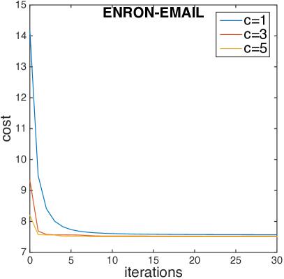
(b) *

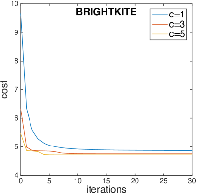
(c) *

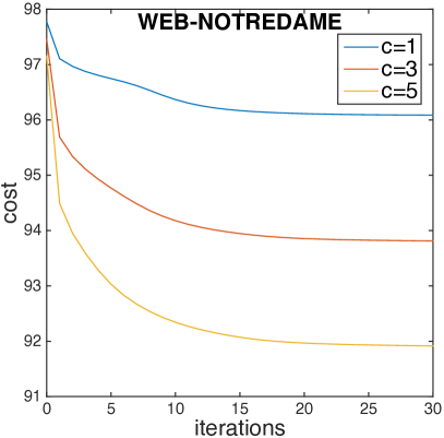
(d) *

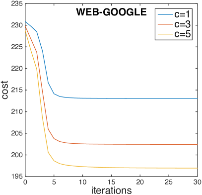
Figure 1: The cost of intermediate $c$-schedules at iterations of wiggins-apx according to $\mathcal{I}$.

Next, we extract the $1$-schedules output by wiggins-apx, and compare its cost to four other natural schedules: unif, outdeg, indeg, and totdeg that probe each node, respectively, uniformly, proportional to its out-degree, proportional to its in-degree, and proportional to the number of incident edges. Note that for undirected graphs outdeg, indeg, and totdeg are essentially the same schedule.

To have a fair comparison among the costs of these schedules and wiggins-apx, we calculate their costs according to 10 independent samples, $\mathcal{I}_{1},\ldots,\mathcal{I}_{10}$ that satisfy (12), and compute the average. The results are shown in Table 4, and show that wiggins-apx outperforms the other four schedules.

Dataset	wiggins-apx	uniform	outdeg	indeg	totdeg
Enron-Email	7.55	14.16	9.21	9.21	9.21
Brightkite	4.85	9.64	6.14	6.14	6.14
web-Notredame	96.10	97.78	97.37	97.43	97.40
web-Google	213.15	230.88	230.48	230.47	230.47

Table 4: Comparing the costs of 5 different 1-schedules.

5.1.1 A Test on Convergence to Optimal Schedule

Here, we further invetigate the convergence of wiggins-apx, using an example graph and process for which we know the unique optimal schedule. We study how close the wiggins-apx output is to the optimal schedule when (i) we start from different initial schedules, $\mathsf{p}^{0}$, or (ii) we use samples $\mathcal{I}$’s obtained during time intervals of different lengths.

Suppose $G=(V,E)$ is the complete graph where $V=[n]$. Let $\Gamma=(\mathcal{F},\pi)$ for $\mathcal{F}=\{S\in 2^{[n]}\mid 1\leq|S|\leq 2\}$, and $\pi(S)=\frac{1}{|\mathcal{F}|}$. It is easy to see that $\mathsf{cost}_{\theta}(\mathsf{p})$ is a symmetric function, and thus, the uniform schedule is optimal. Moreover, by Corollary 1 the uniform schedule is the only optimal schedule, since $\{v\}\in\mathcal{F}$ for every $v\in V$. Furthermore, we let $\theta=0.99$ to increase the sample complexity (as in Lemma 3) and make it harder to learn the uniform/optimal schedule.

(a) *

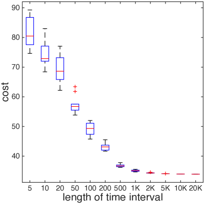
(b) *

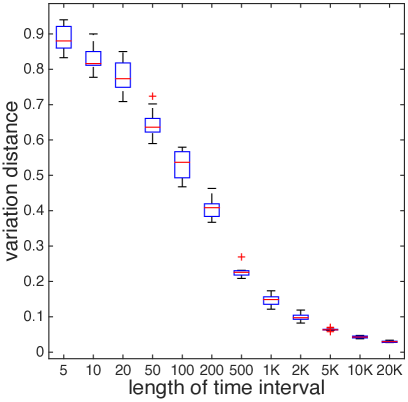
Figure 2: The cost of wiggins-apx outputs and their variation distance to the optimal schedule.

In our experiments we run the wiggins-apx algorithm, using (i) different random initial schedules, and (ii) samples $\mathcal{I}$ obtained from time intervals of different lengths. For each sample, we run wiggins-apx 10 times with 10 different random initial schedules, and compute the exact cost of each schedule, and its variation distance to the uniform schedule. Our results are plotted in Figure 2, and as shown, by increasing the sample size (using longer time intervals of sampling) the output schedules gets very close to the uniform schedule (the variance gets smaller and smaller).

5.2 Dynamic Settings

In this section, we present experimental results that show how our algorithm can adapt itself to the new situation. The experiment is illustrated in Fig. 3. For each graph, we start by following an optimal 1-schedule in the graph. At the beginning of each “gray” time interval, the labels of the nodes are permuted randomly, to impose great disruptions in the system. Following that, at the beginning of each “green” time interval our algorithm starts gathering samples of $\Gamma$. Then, wiggins-apx computes the schedule for the new sample, using 50 rounds of iterations, and starts probing. The length of each colored time interval is $R=\frac{3(\log(n)+\log(2))}{\epsilon^{2}(1-\theta)}$, $\epsilon=0.5$, motivated by Theorem 3.

Since the cost function is defined asymptotically (and explains the asymptotic behavior of the system in response to a schedule), in Figure 3 we plot the load of the system $L_{\theta}(t)$ over the time (blue), and the average load in the normal and perturbed time intervals (red). Based on this experiment, and as shown in Figure 3, after adapting to the new schedule, the effect of the disruption caused by the perturbation disappears immediately. Note that when the difference between the optimal cost and any other schedule is small (like web-Notredame), the jump in the load will be small (e.g., as shown in Figure 1 and Table 4, the cost of the initial schedule for web-Notredame is very close the optimal cost, obtained after 30 iteration).

(a) *

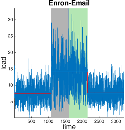
(b) *

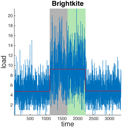
(c) *

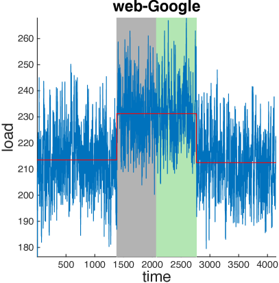
(d) *

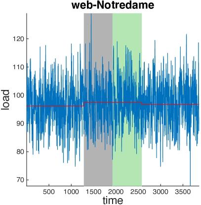
Figure 3: Perturbation, Sampling, and Adapting (For details see Section 5.2).

6 Conclusions

We formulate and study the $(\theta,c)$-Optimal Probing Schedule Problem, which requires to find the best probing schedule that allows an observer to find most pieces of information recently generated by a process $\Gamma$, by probing a limited number of nodes at each time step.

We design and analyze an algorithm, wiggins, that can solve the problem optimally if the parameters of the process $\Gamma$ are known, and then design a variant that computes a high-quality approximation of the optimum schedule when only a sample of the process is available. We also show that wiggins can be adapted to the MapReduce framework of computation, which allows us to scale up to networks with million of nodes. The results of experimental evaluation on a variety of graphs and generating processes show that wiggins and its variants are very effective in practice.

Interesting directions for future work include generalizing the problem to allow for non-memoryless schedules and different novelty functions.

7 Acknowledgements

This work was supported by NSF grant IIS-1247581 and NIH grant R01-CA180776.

References

- Agumbe Suresh et al. [2012] M. Agumbe Suresh, R. Stoleru, R. Denton, E. Zechman, and B. Shihada. Towards optimal event detection and localization in acyclic flow networks. In Proceedings of the 13th International Conference on Distributed Computing and Networking, ICDCN’12, pages 179–196, Berlin, Heidelberg, 2012. Springer-Verlag. ISBN 978-3-642-25958-6. doi: 10.1007/978-3-642-25959-3_13. URL http://dx.doi.org/10.1007/978-3-642-25959-3_13.
- Boyd and Vandenberghe [2004] S. Boyd and L. Vandenberghe. Convex optimization. Cambridge university press, 2004.
- Bright et al. [2006] L. Bright, A. Gal, and L. Raschid. Adaptive pull-based policies for wide area data delivery. ACM Transactions on Database Systems (TODS), 31(2):631–671, 2006.
- Cataldi et al. [2010] M. Cataldi, L. Di Caro, and C. Schifanella. Emerging topic detection on Twitter based on temporal and social terms evaluation. In Proceedings of the Tenth International Workshop on Multimedia Data Mining, MDMKDD ’10, pages 4:1–4:10, New York, NY, USA, 2010. ACM. ISBN 978-1-4503-0220-3. doi: 10.1145/1814245.1814249. URL http://doi.acm.org/10.1145/1814245.1814249.
- Chen et al. [2009] W. Chen, Y. Wang, and S. Yang. Efficient influence maximization in social networks. In Proceedings of the 15th ACM SIGKDD International Conference on Knowledge Discovery and Data Mining, KDD ’09, pages 199–208, New York, NY, USA, 2009. ACM. ISBN 978-1-60558-495-9. doi: 10.1145/1557019.1557047. URL http://doi.acm.org/10.1145/1557019.1557047.
- Chen et al. [2010] W. Chen, C. Wang, and Y. Wang. Scalable influence maximization for prevalent viral marketing in large-scale social networks. In Proceedings of the 16th ACM SIGKDD International Conference on Knowledge Discovery and Data Mining, KDD ’10, pages 1029–1038, New York, NY, USA, 2010. ACM. ISBN 978-1-4503-0055-1. doi: 10.1145/1835804.1835934. URL http://doi.acm.org/10.1145/1835804.1835934.
- Christakis and Fowler [2010] N. A. Christakis and J. H. Fowler. Social network sensors for early detection of contagious outbreaks. PLoS ONE, 5(9):e12948, 2010.
- Dasgupta et al. [2007] A. Dasgupta, A. Ghosh, R. Kumar, C. Olston, S. Pandey, and A. Tomkins. The discoverability of the web. In Proceedings of the 16th international conference on World Wide Web, pages 421–430. ACM, 2007.
- Dean and Ghemawat [2008] J. Dean and S. Ghemawat. Mapreduce: simplified data processing on large clusters. Communications of the ACM, 51(1):107–113, 2008.
- Delaney [2009] A. Delaney. The Growing Role of News in Trading Automation, Oct. 2009. http://www.machinereadablenews.com/images/dl/Machine_Readable_News_and_Algorithmic_Trading.pdf.
- Golovin et al. [2010] D. Golovin, M. Faulkner, and A. Krause. Online distributed sensor selection. In Proceedings of the 9th ACM/IEEE International Conference on Information Processing in Sensor Networks, IPSN ’10, pages 220–231, New York, NY, USA, 2010. ACM. ISBN 978-1-60558-988-6. doi: 10.1145/1791212.1791239. URL http://doi.acm.org/10.1145/1791212.1791239.
- Hardy [1991] G. H. Hardy. Divergent series, volume 334. American Mathematical Soc., 1991.
- Hart and Murray [2010] W. Hart and R. Murray. Review of sensor placement strategies for contamination warning systems in drinking water distribution systems. Journal of Water Resources Planning and Management, 136(6):611–619, 2010. doi: 10.1061/(ASCE)WR.1943-5452.0000081. URL http://ascelibrary.org/doi/abs/10.1061/%28ASCE%29WR.1943-5452.0000081.
- Hope [2015] B. Hope. How computers trawl a sea of data for stock picks. The Wall Street Journal, Apr. 2015. http://www.wsj.com/articles/how-computers-trawl-a-sea-of-data-for-stock-picks-1427941801?KEYWORDS=computers+trawl+sea.
- Horincar et al. [2014] R. Horincar, B. Amann, and T. Artières. Online refresh strategies for content based feed aggregation. World Wide Web, pages 1–35, 2014.
- Jung et al. [2011] K. Jung, W. Heo, and W. Chen. IRIE: Scalable and robust influence maximization in social networks. arXiv preprint arXiv:1111.4795, 2011.
- Kempe et al. [2003] D. Kempe, J. Kleinberg, and E. Tardos. Maximizing the spread of influence through a social network. In Proceedings of the Ninth ACM SIGKDD International Conference on Knowledge Discovery and Data Mining, KDD ’03, pages 137–146, New York, NY, USA, 2003. ACM. ISBN 1-58113-737-0. doi: 10.1145/956750.956769. URL http://doi.acm.org/10.1145/956750.956769.
- Kempe et al. [2005] D. Kempe, J. Kleinberg, and E. Tardos. Influential nodes in a diffusion model for social networks. In Proceedings of the 32Nd International Conference on Automata, Languages and Programming, ICALP’05, pages 1127–1138, Berlin, Heidelberg, 2005. Springer-Verlag. ISBN 3-540-27580-0, 978-3-540-27580-0. doi: 10.1007/11523468_91. URL http://dx.doi.org/10.1007/11523468_91.
- Krause and Guestrin [2011] A. Krause and C. Guestrin. Submodularity and its applications in optimized information gathering. ACM Trans. Intell. Syst. Technol., 2(4):32:1–32:20, July 2011. ISSN 2157-6904. doi: 10.1145/1989734.1989736. URL http://doi.acm.org/10.1145/1989734.1989736.
- Krause et al. [2008] A. Krause, J. Leskovec, C. Guestrin, J. VanBriesen, and C. Faloutsos. Efficient sensor placement optimization for securing large water distribution networks. Journal of Water Resources Planning and Management, 134(6):516–526, 2008. doi: 10.1061/(ASCE)0733-9496(2008)134:6(516). URL http://ascelibrary.org/doi/abs/10.1061/%28ASCE%290733-9496%282008%29134%3A6%28516%29.
- Krause et al. [2009] A. Krause, R. Rajagopal, A. Gupta, and C. Guestrin. Simultaneous placement and scheduling of sensors. In Proceedings of the 2009 International Conference on Information Processing in Sensor Networks, IPSN ’09, pages 181–192, Washington, DC, USA, 2009. IEEE Computer Society. ISBN 978-1-4244-5108-1. URL http://dl.acm.org/citation.cfm?id=1602165.1602183.
- Krause et al. [2011] A. Krause, C. Guestrin, A. Gupta, and J. Kleinberg. Robust sensor placements at informative and communication-efficient locations. ACM Trans. Sen. Netw., 7(4):31:1–31:33, Feb. 2011. ISSN 1550-4859. doi: 10.1145/1921621.1921625. URL http://doi.acm.org/10.1145/1921621.1921625.
- Latar [2015] N. L. Latar. The robot journalist in the age of social physics: The end of human journalism? In The New World of Transitioned Media, pages 65–80. Springer, 2015.
- Leskovec et al. [2007] J. Leskovec, A. Krause, C. Guestrin, C. Faloutsos, J. M. VanBriesen, and N. S. Glance. Cost-effective outbreak detection in networks. In P. Berkhin, R. Caruana, and X. Wu, editors, KDD, pages 420–429. ACM, 2007. ISBN 978-1-59593-609-7.
- Mathioudakis and Koudas [2010] M. Mathioudakis and N. Koudas. Twittermonitor: Trend detection over the twitter stream. In Proceedings of the 2010 ACM SIGMOD International Conference on Management of Data, SIGMOD ’10, pages 1155–1158, New York, NY, USA, 2010. ACM. ISBN 978-1-4503-0032-2. doi: 10.1145/1807167.1807306. URL http://doi.acm.org/10.1145/1807167.1807306.
- McKinney [2011] W. McKinney. Structured Data Challenges in Finance and Statistics, Nov. 2011. http://www.slideshare.net/wesm/structured-data-challenges-in-finance-and-statistics.
- Mitzenmacher and Upfal [2005] M. Mitzenmacher and E. Upfal. Probability and Computing: Randomized Algorithms and Probabilistic Analysis. Cambridge University Press, 2005.
- Oita and Senellart [2011] M. Oita and P. Senellart. Deriving dynamics of web pages: A survey. In TWAW (Temporal Workshop on Web Archiving), 2011.
- Ostfeld et al. [2008] A. Ostfeld, J. Uber, E. Salomons, J. Berry, W. Hart, C. Phillips, J. Watson, G. Dorini, P. Jonkergouw, Z. Kapelan, F. di Pierro, S. Khu, D. Savic, D. Eliades, M. Polycarpou, S. Ghimire, B. Barkdoll, R. Gueli, J. Huang, E. McBean, W. James, A. Krause, J. Leskovec, S. Isovitsch, J. Xu, C. Guestrin, J. VanBriesen, M. Small, P. Fischbeck, A. Preis, M. Propato, O. Piller, G. Trachtman, Z. Wu, and T. Walski. The battle of the water sensor networks (BWSN): A design challenge for engineers and algorithms. Journal of Water Resources Planning and Management, 134(6):556–568, 2008. doi: 10.1061/(ASCE)0733-9496(2008)134:6(556). URL http://ascelibrary.org/doi/abs/10.1061/%28ASCE%290733-9496%282008%29134%3A6%28556%29.
- Sia et al. [2007] K. C. Sia, J. Cho, and H.-K. Cho. Efficient monitoring algorithm for fast news alerts. Knowledge and Data Engineering, IEEE Transactions on, 19(7):950–961, 2007.
- Tang et al. [2014] Y. Tang, X. Xiao, and Y. Shi. Influence maximization: Near-optimal time complexity meets practical efficiency. arXiv preprint arXiv:1404.0900, 2014.
- Wolf et al. [2002] J. L. Wolf, M. S. Squillante, P. Yu, J. Sethuraman, and L. Ozsen. Optimal crawling strategies for web search engines. In Proceedings of the 11th international conference on World Wide Web, pages 136–147. ACM, 2002.