On Galerkin approximations of the surface-active quasigeostrophic equations

Abstract

We study the representation of solutions of the three-dimensional quasigeostrophic (QG) equations using Galerkin series with standard vertical modes, with particular attention to the incorporation of active surface buoyancy dynamics. We extend two existing Galerkin approaches (A and B) and develop a new Galerkin approximation (C). Approximation A, due to Flierl (1978), represents the streamfunction as a truncated Galerkin series and defines the potential vorticity (PV) that satisfies the inversion problem exactly. Approximation B, due to Tulloch and Smith (2009b), represents the PV as a truncated Galerkin series and calculates the streamfunction that satisfies the inversion problem exactly. Approximation C, the true Galerkin approximation for the QG equations, represents both streamfunction and PV as truncated Galerkin series, but does not satisfy the inversion equation exactly. The three approximations are fundamentally different unless the boundaries are isopycnal surfaces. We discuss the advantages and limitations of approximations A, B, and C in terms of mathematical rigor and conservation laws, and illustrate their relative efficiency by solving linear stability problems with nonzero surface buoyancy. With moderate number of modes, B and C have have superior accuracy than A at high wavenumbers. Because B lacks conservation of energy, we recommend approximation C for constructing solutions to the surface-active QG equations using Galerkin series with standard vertical modes.

1 Introduction

Recent interest in upper-ocean dynamics and sub-mesoscale turbulence has focussed attention on surface geostrophic dynamics and the role of surface buoyancy variations. A main issue is the representation of active surface buoyancy by finite vertical truncations of the quasigeostrophic (QG) equations. Standard multi-layer (e.g., Pedlosky 1987) and modal approximations (e.g., Flierl 1978) assume that there is no variation of buoyancy on the surfaces.

Here we explore the representation of surface and interior dynamics using the simple and familiar vertical modes of physical oceanography. These modes, denoted here by $\mathsf{p}_{n}(z)$, are defined by the Sturm-Liouville eigenproblem

$$\frac{{\rm d}}{{\rm d}z}\frac{f_{0}^{2}}{N^{2}}\frac{{\rm d}\mathsf{p}_{n}}{{\rm d}z}=-\kappa_{n}^{2}\mathsf{p}_{n}\,,$$ (1)

with homogeneous Neumann boundary conditions at the bottom ($z=z^{-}$) and top ($z=z^{+}$) surfaces of the domain:

$$\frac{{\rm d}\mathsf{p}_{n}}{{\rm d}z}\left(z^{\pm}\right)=0\,.$$ (2)

In (1) $N$ is the buoyancy frequency and $f_{0}$ is the Coriolis parameter. The eigenvalue $\kappa_{n}$ in (1) is the deformation wavenumber of the $n$’th mode. With normalization, the modes satisfy the orthogonality condition

$$\tfrac{1}{h}\int_{z^{-}}^{z^{+}}\!\!\!\mathsf{p}_{n}\mathsf{p}_{m}\,{\rm d}z=\delta_{mn}\,,$$ (3)

where $h\stackrel{{\scriptstyle\mathrm{def}}}{{=}}z^{+}-z^{-}$ is the depth. The barotropic mode is $\mathsf{p}_{0}=1$ and $\kappa_{0}=0$.

The modes defined by the eigenproblem (1) and (2) provide a fundamental basis for representing solutions of both the primitive and quasigeostrophic equations as a linear combination of $\{\mathsf{p}_{n}\}$ (Gill 1982; Pedlosky 1987; Vallis 2006; Ferrari and Wunsch 2010; LaCasce 2012). In fact, the set $\{\mathsf{p}_{n}\}$ is mathematically complete and can be used to represent any field with finite square integral,

$$\int_{z^{-}}^{z^{+}}\!\!\!\!\phi^{2}\,{\rm d}z<\infty\,.$$ (4)

Even if the field $\phi$ has nonzero derivative at $z^{\pm}$, or internal discontinuities, its representation as a linear combination of the basis functions $\{\mathsf{p}_{n}\}$ converges in $L^{2}(z^{-},z^{+})$ i.e., the integral of the squared error goes to zero as the number of basis functions increases (e.g., Hunter and Nachtergaele 2001, ch. 10).

Despite the rigorous assurance of completeness in the previous paragraph, the utility of $\{\mathsf{p}_{n}\}$ for problems with nonuniform surface buoyancy has been questioned by several authors (e.g., Lapeyre 2009; Roullet et al. 2012; Smith and Vanneste 2013). These authors argue that the homogeneous boundary conditions in (2) are incompatible with non-zero surface buoyancy and that representation of the streamfunction $\psi$ as a linear combination of $\{\mathsf{p}_{n}\}$ is useless if $\psi_{z}$ is non-zero on the surfaces. This supposed incompatibility of (2) with non-zero surface buoyancy is a main motivation for a new, alternative set of orthogonal basis functions proposed by Smith and Vanneste (2013).

The aim of this paper is to obtain a good Galerkin approximation to solutions of the QG equation with non-zero surface buoyancy using the familiar basis $\{\mathsf{p}_{n}\}$. We show that that both the inversion problem and evolutionary dynamics can be handled using $\{\mathsf{p}_{n}\}$ to represent the streamfunction. As part of this program we revisit and extend two existing modal approximations (Flierl 1978; Tulloch and Smith 2009a), and develop a new Galerkin approximation. We discuss the relative merit of the three approximations in terms of their mathematical rigor and conservation laws, and illustrate their efficiency and caveats by solving linear stability problems with nonzero surface buoyancy.

Using concrete examples, we show that the concerns expressed by earlier authors regarding the suitability of the standard modes $\{\mathsf{p}_{n}\}$ are over-stated: even with non-zero surface buoyancy, the Galerkin expansion for $\psi$ in terms of $\{\mathsf{p}_{n}\}$ converges absolutely and uniformly with no Gibbs phenomena. A modest number of terms provides a good approximation to $\psi$ throughout the domain, including on the top and bottom boundaries. In other words, the surface streamfunction can be expanded in terms of $\{\mathsf{p}_{n}\}$ and, with enough modes, this representation can then be used to accurately calculate the advection of non-zero surface buoyancy. In section 5 we illustrate this procedure by solving the classic Eady problem using the basis $\{\mathsf{p}_{n}\}$ for the streamfunction.

2 The exact system

In this section we summarize the basic properties of the QG system. For a detailed derivation see Pedlosky (1987).

2.1 Formulation

The streamfunction is denoted $\psi(x,y,z,t)$ and we use the following notation.

$$u=-\psi_{y}\,,\qquad v=\psi_{x}\,,\qquad\vartheta=\left(\tfrac{f_{0}}{N}\right)^{2}\psi_{z}\,.$$ (5)

The variable $\vartheta$ is related to the buoyancy by $b=N^{2}\vartheta/f_{0}$. The QG potential vorticity (QGPV) equation is

$$\partial_{t}q+\mathsf{J}(\psi,q)+\beta v=0\,,$$ (6)

where the potential vorticity is

$$q=\left(\triangle+\mathsf{L}\right)\psi\,,$$ (7)

with

$$\triangle\stackrel{{\scriptstyle\mathrm{def}}}{{=}}\partial_{x}^{2}+\partial_{y}^{2}\,,\qquad\text{and}\qquad\mathsf{L}\stackrel{{\scriptstyle\mathrm{def}}}{{=}}\partial_{z}\left(\tfrac{f_{0}}{N}\right)^{2}\partial_{z}\,.$$ (8)

Also in (6), the Jacobian is $\mathsf{J}(A,B)\stackrel{{\scriptstyle\mathrm{def}}}{{=}}\partial_{x}A\,\partial_{y}B-\partial_{y}A\,\partial_{x}B$.

The boundary conditions at the top ($z=z^{+}$) and bottom ($z=z^{-}$) are that $w=0$, or equivalently

$$@z=z^{\pm}\,:\qquad\partial_{t}\vartheta^{\pm}+\mathsf{J}(\psi^{\pm},\vartheta^{\pm})=0\,.$$ (9)

Above we have used the superscripts $+$ and $-$ to denote evaluation at $z^{+}$ and $z^{-}$ e.g., $\psi^{+}=\psi(x,y,z^{+},t)$.

2.2 Quadratic conservation laws

In the absence of sources and sinks, the exact QG system has four quadratic conservation laws: energy, potential enstrophy, and surface buoyancy variance at the two surfaces (e.g., Pedlosky 1987; Vallis 2006). Throughout we assume horizontal periodic boundary conditions.

The well-known energy conservation law is

$$\frac{dE}{dt}=0\,,$$ (10)

where

$$E\stackrel{{\scriptstyle\mathrm{def}}}{{=}}\int\tfrac{1}{2}|\bm{\nabla}\psi|^{2}+\tfrac{1}{2}\left(\tfrac{f_{0}}{N}\right)^{2}\!\left(\partial_{z}\psi\right)^{2}\,{\rm d}V\,.$$ (11)

The total energy is $\rho_{0}\,E$, where $\rho_{0}$ is a reference density. An alternative expression for $E$ is

$$E=-\tfrac{1}{2}\int\!\!\psi q\,{\rm d}V+\tfrac{1}{2}\int\!\psi^{\mathrm{+}}\vartheta^{\mathrm{+}}-\psi^{\mathrm{-}}\vartheta^{\mathrm{-}}{\rm d}S\,.$$ (12)

If $q=0$ (e.g., as in the Eady problem) then (12) expresses $E$ in terms of surface contributions.

If $\beta=0$ then there are many quadratic potential enstrophy invariants: the volume integral of $q^{2}A(z)$, with $A(z)$ an arbitrary function of the vertical coordinate, is conserved. The choice $A(z)=\delta(z-z_{*})$ reduces to conservation of the surface integral of $q^{2}$ at any level $z_{*}$.

Charney (1971) noted that, in a doubly periodic domain, nonzero $\beta$ destroys all these quadratic potential enstrophy conservation laws, including the conservation of potential enstrophy defined simply as the volume integral of $q^{2}$. Multiplying the QGPV equation (6) by $q$, and integrating by parts, we obtain

$$\frac{{\rm d}}{{\rm d}t}\int\tfrac{1}{2}q^{2}\,{\rm d}V+\beta\int\big{[}v\vartheta\big{]}_{z^{-}}^{z^{+}}\,{\rm d}S=0\,.$$ (13)

The potential enstrophy equation (13) is the finite-depth analog of Charney’s equation (13). To make progress Charney assumed $\vartheta=0$ at the ground. But the $\beta$-term on the right of (13) can be eliminated by cross-multiplying the QGPV equation (6) evaluated at the surfaces $z^{\pm}$ with the boundary conditions (9), and combining with (13). Thus nonzero $\beta$ selects a uniquely conserved potential enstrophy from the infinitude of $\beta=0$ potential enstrophy conservation laws:

$$\frac{dZ}{dt}=0\,,$$ (14)

where the potential enstrophy is

$$Z\stackrel{{\scriptstyle\mathrm{def}}}{{=}}\int\tfrac{1}{2}q^{2}\,{\rm d}V-\int q^{+}\vartheta^{\mathrm{+}}-q^{-}\vartheta^{\mathrm{-}}\,{\rm d}S\,.$$ (15)

With $\beta\neq 0$ the surface contributions in (15) are required to form a conserved quadratic quantity involving $q^{2}$. Notice that (15) is not sign-definite. To our knowledge, the conservation law in (14) and (15) is previously unremarked.

Finally, in addition to $E$ and $Z$, the surface buoyancy variance is conserved on each surface

$$\frac{{\rm d}}{{\rm d}t}\int\tfrac{1}{2}\left(\vartheta^{\pm}\right)^{2}{\rm d}S=0\,.$$ (16)

Thus, with $\beta\neq 0$, the QG model has four quadratic conservation laws: $E$, $Z$ and the buoyancy variance at the two surfaces.

3 Galerkin approximation using standard vertical modes

A straightforward approach is to represent the streamfunction by linearly combining the first $\mathrm{N}+1$ vertical modes. The mean square error in this approximation is

$$\text{err}_{\psi}(a_{0},a_{1},\cdots a_{\mathrm{N}})\stackrel{{\scriptstyle\mathrm{def}}}{{=}}\frac{1}{h}\int_{z^{-}}^{z^{+}}\Big{(}\psi-\sum_{n=0}^{\mathrm{N}}a_{n}\mathsf{p}_{n}\Big{)}^{2}\,{\rm d}z\,.$$ (17)

We use a roman font, and context, to distinguish the truncation index $\mathrm{N}$ in (17) from the buoyancy frequency $N(z)$. The coefficients $a_{0}$ through $a_{\mathrm{N}}$ are determined to minimize $\text{err}_{\psi}$, and thus one obtains the Galerkin approximation $\psi^{\mathrm{G}}_{\mathrm{N}}$ to the exact streamfunction:

$$\psi^{\mathrm{G}}_{\mathrm{N}}(x,y,z,t)\stackrel{{\scriptstyle\mathrm{def}}}{{=}}\sum_{n=0}^{\mathrm{N}}\breve{\psi}_{n}(x,y,t)\mathsf{p}_{n}(z)\,,$$ (18)

where the coefficients in the sum above are

$$\breve{\psi}_{n}(x,y,t)\stackrel{{\scriptstyle\mathrm{def}}}{{=}}\tfrac{1}{h}\int_{z^{-}}^{z^{+}}\!\!\!\!\psi\,\mathsf{p}_{n}\,{\rm d}z\,.$$ (19)

Throughout we use the superscript $\breve{}$ to denote a Galerkin coefficient defined via projection of a field onto a vertical mode.

In complete analogy with the streamfunction, one can also develop an $(\mathrm{N}+1)$-mode Galerkin approximation to the PV:

$$q^{\mathrm{G}}_{\mathrm{N}}(x,y,z,t)\stackrel{{\scriptstyle\mathrm{def}}}{{=}}\sum_{n=0}^{\mathrm{N}}\breve{q}_{n}(x,y,t)\mathsf{p}_{n}(z)\,,$$ (20)

with coefficients

$$\breve{q}_{n}\stackrel{{\scriptstyle\mathrm{def}}}{{=}}\tfrac{1}{h}\int_{z^{-}}^{z^{+}}\!\!\!\!q\,\mathsf{p}_{n}\,{\rm d}z\,.$$ (21)

The construction of the Galerkin approximation $q^{\mathrm{G}}_{\mathrm{N}}$ above minimizes a mean square error $\text{err}_{q}$ defined in analogy with (17).

Now recall that the exact $\psi$ and $q$ are related by the elliptic “inversion problem”:

$$(\triangle+\mathsf{L})\psi=q\,,$$ (22)

with boundary conditions at $z^{\pm}$:

$$\left(\tfrac{f_{0}}{N}\right)^{2}\psi_{z}=\vartheta^{\pm}\,.$$ (23)

The Galerkin approximations in (18) through (21) are defined independently of the information in (22) and (23). The relationship between the Galerkin coefficients $\breve{q}_{n}$ and $\breve{\psi}_{n}$ is obtained by multiplying (22) by $\tfrac{1}{h}\mathsf{p}_{n}(z)$ and integrating over the depth. Noting the intermediate result

$$\tfrac{1}{h}\int_{z^{-}}^{z^{+}}\!\!\!\mathsf{p}_{n}\mathsf{L}\psi\,{\rm d}z=\tfrac{1}{h}\left[\mathsf{p}_{n}^{+}\vartheta^{\mathrm{+}}-\mathsf{p}_{n}^{-}\vartheta^{\mathrm{-}}\right]-\kappa_{n}^{2}\breve{\psi}_{n}\,,$$ (24)

we obtain

$$\breve{q}_{n}=\triangle_{n}\breve{\psi}_{n}+\underbrace{\tfrac{1}{h}\left(\mathsf{p}_{n}^{+}\,\vartheta^{\mathrm{+}}-\mathsf{p}_{n}^{-}\,\vartheta^{\mathrm{-}}\right)}_{\text{surface terms}}\,,$$ (25)

where $\triangle_{n}$ is the $n$’th mode Helmholtz operator

$$\triangle_{n}\stackrel{{\scriptstyle\mathrm{def}}}{{=}}\triangle-\kappa^{2}_{n}\,.$$ (26)

The relation in (25) is the key to a good Galerkin approximation to surface-active quasigeostrophic dyamics.

Term-by-term differentiation of the $\psi^{\mathrm{G}}_{\mathrm{N}}$-series in (18) does not give the $q^{\mathrm{G}}_{\mathrm{N}}$ series in (20) unless $\vartheta^{\pm}=0$. In other words, term-by-term differentiation does not produce the correct relation (25) between $\breve{q}_{n}$ and $\breve{\psi}_{n}$. Thus the Galerkin truncated PV and the Galerkin truncated streamfunction do not satisfy the inversion boundary value problem exactly

$$\big{(}\triangle+\mathsf{L}\big{)}\psi^{\mathrm{G}}_{\mathrm{N}}\neq q^{\mathrm{G}}_{\mathrm{N}}\,.$$ (27)

Despite (27), the truncated series $\psi^{\mathrm{G}}_{\mathrm{N}}$ and $q^{\mathrm{G}}_{\mathrm{N}}$ are the best least-squares approximations to $\psi$ and $q$.

Notice that, in analogy with the Galerkin approximations for $q$ and $\psi$,

$$\breve{\delta}^{+}_{n}=\tfrac{1}{h}\mathsf{p}_{n}^{+}\qquad\text{and}\qquad\breve{\delta}^{-}_{n}=\tfrac{1}{h}\mathsf{p}_{n}^{-}\,,$$ (28)

where

$$\delta_{\mathrm{N}}^{+G}(z)=\sum_{n=0}^{\mathrm{N}}\breve{\delta}^{+}_{n}\mathsf{p}_{n}\qquad\text{and}\qquad\delta_{\mathrm{N}}^{-G}(z)=\sum_{n=0}^{\mathrm{N}}\breve{\delta}^{-}_{n}\mathsf{p}_{n}\,,$$ (29)

are finite approximations to distributions $\delta(z-z^{\pm})$ at the surfaces. Of course, these surface $\delta$-distributions do not satisfy the $L^{2}$ convergence condition in (4) and thus the series in (29) only converge in a distributional sense.(e.g., Hunter and Nachtergaele 2001). For instance, if $\phi$ satisfies the $L^{2}$ convergence condition in (4), then

$$\int_{z^{-}}^{z^{+}}\!\!\phi(z)\delta_{\mathrm{N}}^{+G}(z)\,{\rm d}z\,\,\to\,\int_{z^{-}}^{z^{+}}\!\!\phi(z)\delta(z-z^{+})\,{\rm d}z=\phi(z^{+})\,,$$ (30)

as $\mathrm{N}\to\infty$. Thus, in that limit,

$$\big{(}\triangle+\mathsf{L}\big{)}\psi^{\mathrm{G}}_{\mathrm{N}}\rightharpoonup q-\delta(z-z^{+})\,\vartheta^{\mathrm{+}}+\delta(z-z^{-})\,\vartheta^{\mathrm{-}}\,,$$ (31)

where $\rightharpoonup$ denotes distributional convergence. The right-hand-side of (31) is the Brethertonian modified potential vorticity (Bretherton 1966) with the boundary conditions incorporated as PV sheets. To illustrate (27) and (31) we present an elementary example that is is relevant to our discussion of the Eady problem in section 5.

An elementary example: the Eady basic state

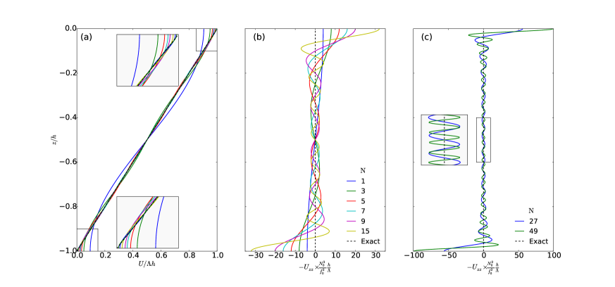
Figure 1: Nondimensional base-state for the Eady problem using various truncation for the series (34). In the middle panel $\mathrm{N}$ is the number of baroclinic modes. (a) Zonal velocity: although the truncation has zero slope at the boundaries there are no Gibbs oscillations. (b) Meridional PV gradient associated with the truncated series (36). (c) as in (b) but with an expanded abscissa. As $\mathrm{N}$ increases, the PV gradient distributionally converges to two Brethertonian delta functions at the boundaries.

As an example, consider the case with constant buoyancy frequency $N$. We use nondimensional units so that the surfaces are at $z^{-}=-1$ and $z^{+}=0$. The standard vertical modes are $\mathsf{p}_{0}=1$ and, for $n\geq 1$

$$\mathsf{p}_{n}=\sqrt{2}\cos(n\pi z)\,,$$ (32)

with $\kappa_{n}=n\pi$.

We consider the basic state of the Eady problem with streamfunction

$$\psi=-\underbrace{(1+z)}_{U}y\,,$$ (33)

and zero interior PV $q=0$ and $\beta=0$. The surface buoyancies are $\vartheta^{\pm}=-y$.

The Galerkin expansion of the PV $q=0$ is exact: $\breve{q}_{\mathrm{N}}=0$ and therefore $q^{\mathrm{G}}_{\mathrm{N}}=0$. The truncated Galerkin expansion of $\psi$ follows from either (19) or (25) and is

$$\psi^{\mathrm{G}}_{\mathrm{N}}=-\underbrace{\left[\tfrac{1}{2}\mathsf{p}_{0}+2\sqrt{2}\left(\frac{\mathsf{p}_{1}}{\pi^{2}}+\frac{\mathsf{p}_{3}}{(3\pi)^{2}}+\cdots+\frac{\mathsf{p}_{\mathrm{N}}}{(\mathrm{N}\pi)^{2}}\right)\right]}_{U^{\mathrm{G}}_{\mathrm{N}}}y\,.$$ (34)

(We assume that $\mathrm{N}$ is odd, so that the last term in the truncated series is as above.) Despite the nonzero derivative of $\psi$ at the boundaries, the series in (34) is absolutely and uniformly convergent on the closed interval $-1\leq z\leq 0$. The $\mathrm{N}^{-2}$ behavior of the series (34) ensures uniform convergence, e.g., using the M-test (Hunter and Nachtergaele 2001). There are no Gibbs oscillations and a modest number of terms provides a good approximation to the base velocity $U$ (Figure 1a).

Now, to illustrate (27) and (31), notice that

$$\left(\triangle+\mathsf{L}\right)\psi^{\mathrm{G}}_{\mathrm{N}} =2\sqrt{2}\left(\mathsf{p}_{1}+\mathsf{p}_{3}+\cdots\mathsf{p}_{\mathrm{N}}\right)y$$ (35)

$$=2\,\frac{\sin\left[(\mathrm{N}+1)\pi z\right]}{\sin(\pi z)}\,y\,.$$ (36)

The series (35) does not converge in a pointwise sense. However, in a distributional sense (Hunter and Nachtergaele 2001, ch. 11), the exact sum in (36) does converge to $\delta$-distributions on the boundaries; see figures 1(b) and 1(c). These boundary $\delta$-distributions are the Brethertonian PV sheets (Bretherton 1966).

4 Three approximations

In (27) we noted that the Galerkin approximations to $\psi$ and $q$ do not exactly satisfy the inversion relation. To address this error there are at least three different approximations one can make:

Approximation A: Use the truncated sum $\psi^{\mathrm{G}}_{\mathrm{N}}$ in (18) as a least-squares Galerkin approximation to the streamfunction $\psi$. But do not use the Galerkin approximation for $q$. Instead, define the approximate PV, $q^{A}_{\mathrm{N}}(x,y,z,t)$, so that the interior inversion relation is satisfied exactly:

$$q^{A}_{\mathrm{N}}\stackrel{{\scriptstyle\mathrm{def}}}{{=}}\big{(}\triangle+\mathsf{L}\big{)}\psi^{\mathrm{G}}_{\mathrm{N}}\,.$$ (37)

This is the approximation introduced by Flierl (1978), which is now regarded as the standard in physical oceanography. Note that $q^{A}_{\mathrm{N}}$ in (37) is not the least-squares approximation to the exact $q$. Moreover, the approximation $q^{A}_{\mathrm{N}}$ approaches the Brethertonian PV on the right of (31) as $\mathrm{N}\to\infty$.

Approximation B: Use the truncated sum $q^{\mathrm{G}}_{\mathrm{N}}$ in (20) as a least-squares Galerkin approximation to the PV $q$. But do not use the Galerkin approximation for $\psi$. Instead, define the approximate streamfunction, $\psi^{B}_{\mathrm{N}}(x,y,z,t)$, as the solution to the inversion boundary value problem

$$\big{(}\triangle+\mathsf{L}\big{)}\psi^{B}_{\mathrm{N}}=q^{\mathrm{G}}_{\mathrm{N}}\,,$$ (38)

with boundary conditions

$$\left(\tfrac{f_{0}}{N}\right)^{2}\partial_{z}\psi^{B}_{\mathrm{N}}=\vartheta^{\pm}\,.$$ (39)

This is the approximation introduced by Tulloch and Smith (2009b). Notice that (38) and (39) is an approximation to the exact inversion problem because the interior source is $q^{\mathrm{G}}_{\mathrm{N}}$, rather than $q$. In other words, $\psi^{B}_{\mathrm{N}}$ is an exact solution to an approximate version of the inversion problem. But $\psi^{B}_{\mathrm{N}}$ is not a least-squares approximation to the exact $\psi$, and nor can $\psi^{B}_{\mathrm{N}}$ be written as a finite sum of vertical modes.

Approximation C: Use truncated Galerkin approximations $\psi^{\mathrm{G}}_{\mathrm{N}}$ and $q^{\mathrm{G}}_{\mathrm{N}}$ for both $\psi$ and $q$. In this case, as indicated in (27), the inversion equation will not be satisfied exactly by the approximate streamfunction and PV. But instead, one will have true least-squares approximations to both $\psi$ and $q$. To our knowledge approximation C, correctly accounting for the surface-buoyancy boundary terms, has not been previously investigated.

In approximation A there are $\mathrm{N}+1$ modal amplitudes. In approximations B and C there are $\mathrm{N}+3$ degrees of freedom: the $\mathrm{N}+1$ modal amplitudes $\breve{q}_{n}$ and the two surface buoyancy fields $\vartheta^{\pm}$. The three approximations are equivalent when $\vartheta^{\pm}=0$. Approximation C is a true Galerkin approximation and it is important to understand its limitations and advantages relative to the better known alternatives A and B.

Once an approximation has been chosen, one needs to construct evolution equations for the Galerkin coefficients using the QG equations (6) and (9). In the next three sub-sections, we derive evolution equations and the associated inviscid conservation laws for the three approximations outlined above. After testing, we recommend C as the most reliable approximation using standard vertical modes.

4.1 Approximation A

Following Flierl (1978), in approximation A the $\mathrm{N}$-mode approximate PV is defined via (37) and, using the modal representation for $\psi^{\mathrm{G}}_{\mathrm{N}}$ in (18), this is equivalent to

$$q^{A}_{\mathrm{N}}\stackrel{{\scriptstyle\mathrm{def}}}{{=}}\sum_{n=0}^{\mathrm{N}}\triangle_{n}\breve{\psi}_{n}(x,y,t)\,\mathsf{p}_{n}(z)\,,$$ (40)

where $\triangle_{n}$ is the Helmholtz operator in (26). Following the appendix of Flierl (1978), one can use Galerkin projection of the nonlinear evolution equation (6) onto the modes $\mathsf{p}_{n}$ to obtain $\mathrm{N}+1$ evolution equations for the coefficients $\breve{\psi}_{n}$:

$$\partial_{t}\triangle_{n}\breve{\psi}_{n}+\sum_{m=0}^{\mathrm{N}}\sum_{s=0}^{\mathrm{N}}\Xi_{nms}\,\mathsf{J}\left(\breve{\psi}_{m},\triangle_{s}\breve{\psi}_{s}\right)+\beta\partial_{x}\breve{\psi}_{n}=0\,,$$ (41)

where

$$\Xi_{nms}\stackrel{{\scriptstyle\mathrm{def}}}{{=}}\tfrac{1}{h}\int_{z^{-}}^{z^{+}}\!\!\mathsf{p}_{n}\mathsf{p}_{m}\mathsf{p}_{s}\,{\rm d}z\,.$$ (42)

Note that $\Xi_{nms}$ cannot be computed exactly except in cases with simple buoyancy frequency profiles. But it suffices to compute $\Xi_{nms}$ to high accuracy, e.g. using Gaussian quadrature.

Flierl (1978) implicitly assumed that $\vartheta^{+}=\vartheta^{-}=0$, so that the surface terms in (25) vanish and then there is no difference between $q^{A}_{\mathrm{N}}$ and $q^{\mathrm{G}}_{\mathrm{N}}$. But in general, with nonzero surface buoyancy, we can append evolution equations for $\vartheta^{\mathrm{+}}$ and $\vartheta^{\mathrm{-}}$ to approximation A. That is, in addition to the $\mathrm{N}+1$ modal equations in (41), we also have

$$\partial_{t}\vartheta^{\pm}+\sum_{n=0}^{\mathrm{N}}\mathsf{p}_{n}^{\pm}\,\mathsf{J}(\breve{\psi}_{n},\vartheta^{\pm})=0\,.$$ (43)

Above we have evaluated the $\psi$-series (18) at $z^{\pm}$ to approximate $\psi^{\pm}$ in the surface boundary conditions. This approach is not satisfactory because the resulting surface buoyancy equations (43) are dynamically passive i.e., $\vartheta^{+}$ and $\vartheta^{-}$ do not affect the interior evolution equations in (41).

Quadratic conservation laws

Appendix A shows that Approximation A has the energy conservation

$$\frac{{\rm d}}{{\rm d}t}\sum_{n=0}^{\mathrm{N}}\int\tfrac{1}{2}(\nabla\breve{\psi}_{n})^{2}+\tfrac{1}{2}\kappa_{n}^{2}\breve{\psi}_{n}^{2}\,\,{\rm d}S=0\,.$$ (44)

To obtain the energy analogous to $E$ in (11), the modal sum above is multiplied by the depth $h$. With $\beta\neq 0$, approximation A has the potential enstrophy conservation law,

$$\frac{{\rm d}}{{\rm d}t}\sum_{n=0}^{\mathrm{N}}\int\tfrac{1}{2}\big{(}\triangle_{n}\breve{\psi}_{n}\big{)}^{2}{\rm d}S=0\,.$$ (45)

With $\beta\neq 0$, the analog of the exact potential enstrophy (15) is not conserved. Finally, with the surface equations in (43), approximation A also conserves surface buoyancy variance as in (16).

4.2 Approximation B

Approximation B begins with the observation that the exact solution of the inversion problem in (22) and (23) can be decomposed as

$$\psi=\phi+\sigma$$ (46)

where $\phi(x,y,z,t)$ is the “interior streamfunction” and $\sigma(x,y,z,t)$ is the “surface streamfunction” (Lapeyre and Klein 2006; Tulloch and Smith 2009b).

The surface streamfunction $\sigma(x,y,z,t)$ is defined as the solution of the boundary value problem

$$\left(\triangle+\mathsf{L}\right)\sigma=0\,,$$ (47)

with inhomogeneous Neumann boundary conditions

$$\left(\tfrac{f_{0}}{N}\right)^{2}\partial_{z}\sigma\left(z^{\pm}\right)=\vartheta^{\pm}\,.$$ (48)

In approximation B, one must always solve for the surface streamfunction using methods other than a truncated series. The solution of the surface problem (47) and (48) in terms of standard vertical modes is

$$\sigma=\sum_{n=0}^{\infty}\breve{\sigma}_{n}(x,y,t)\mathsf{p}_{n}(z)\,,\quad\text{and}\quad\breve{\sigma}_{n}=\tfrac{1}{h}\int_{z^{-}}^{z^{+}}\!\!\!\!\mathsf{p}_{n}\sigma\,{\rm d}z\,.$$ (49)

where

$$\triangle_{n}\breve{\sigma}_{n}=-\tfrac{1}{h}(\mathsf{p}_{n}^{+}\vartheta^{\mathrm{+}}-\mathsf{p}_{n}^{-}\vartheta^{\mathrm{-}})\,,$$ (50)

and $\triangle_{n}$ is the $n$’th mode Helmholtz operator defined in (26). In (49) and (50) we have a solution for the surface streamfunction $\sigma$, with nonzero vertical derivative $\sigma_{z}$ at the surfaces, in terms of vertical modes with zero derivative. Truncations of the series (49) behave similarly to the truncated series (34): convergence is absolute and uniform (see appendix A).

The interior streamfunction $\phi(x,y,z,t)$ is defined as the solution of the boundary value problem

$$\left(\triangle+\mathsf{L}\right)\phi=q\,,$$ (51)

with homogeneous Neumann boundary conditions

$$\left(\tfrac{f_{0}}{N}\right)^{2}\partial_{z}\phi\left(z^{\pm}\right)=0\,.$$ (52)

Approximation B assumes that one can solve the surface problem in (47) and (48) without resorting to truncated versions of the series in (49). For instance, with constant or exponential stratifications one can find closed-form, exact expressions for $\sigma$ (Tulloch and Smith 2009b; LaCasce 2012). In particular, approximation B requires that the two unknown Dirichlet boundary-condition functions $\sigma^{\pm}=\sigma(z^{\pm})$ can be obtained efficiently from specified Neumann boundary-condition functions $\vartheta^{\mathrm{+}}$ and $\vartheta^{\mathrm{-}}$. The Eady problem, discussed below in section 5, is a prime example in which one can obtain this Neumann-to-Dirichlet map.

Once $\sigma$ is in hand, the approximate streamfunction is

$$\psi^{B}_{\mathrm{N}}=\phi^{B}_{\mathrm{N}}+\sigma\,,$$ (53)

where $\phi^{B}_{\mathrm{N}}(x,y,z,t)$ is obtained by solving the interior inversion problem (51) with the right hand side replaced by the Galerkin approximation $q^{\mathrm{G}}_{\mathrm{N}}$ defined in (20) and (21). The exact solution of this approximation to the interior inversion problem is

$$\phi^{B}_{\mathrm{N}}=\sum_{n=0}^{\mathrm{N}}\breve{\phi}_{n}(x,y,t)\mathsf{p}_{n}(z)\,,$$ (54)

where

$$\breve{\phi}_{n}\stackrel{{\scriptstyle\mathrm{def}}}{{=}}\tfrac{1}{h}\int_{z^{-}}^{z^{+}}\!\!\!\!\mathsf{p}_{n}\phi\,{\rm d}z\,,\qquad\text{and}\qquad\triangle_{n}\breve{\phi}_{n}=\breve{q}_{n}\,.$$ (55)

To obtain the approximation B evolution equations we introduce the streamfunction (53) into the QGPV equation (6) and project onto mode $n$ to obtain

$$\partial_{t}\triangle_{n}\breve{\phi}_{n}+\sum_{m=0}^{\mathrm{N}} \sum_{s=0}^{\mathrm{N}}\Xi_{nms}\,\mathsf{J}\left(\breve{\phi}_{m},\triangle_{s}\breve{\phi}_{s}\right)+\beta\partial_{x}\left(\breve{\phi}_{n}+\breve{\sigma}_{n}\right)$$

$$+\sum_{s=0}^{\mathrm{N}}\tfrac{1}{h}\int_{z^{-}}^{z^{+}}\!\!\!\!\mathsf{p}_{n}\mathsf{p}_{s}\mathsf{J}\left(\sigma\,,\triangle_{s}\breve{\phi}_{s}\right)\,{\rm d}z=0\,,$$ (56)

with $\Xi_{nms}$ defined in (42). Approximation B assumes that the remaining integral on the second line of (56) can be evaluated exactly. This is only possible for particular models of the $N(z)$ (e.g., constant buoyancy-frequency profiles). In practice, however, it may suffice to compute the integral on the second line (56) very accurately, e.g. using Gaussian quadrature.

The evolution equations for approximation B are completed with the addition of buoyancy-advection at the surfaces

$$\partial_{t}\vartheta^{\pm}+\mathsf{J}(\sigma^{\pm},\vartheta^{\pm})+\sum_{n=0}^{\mathrm{N}}\,\mathsf{p}_{n}^{\pm}\mathsf{J}(\breve{\phi}_{n},\vartheta^{\pm})=0\,.$$ (57)

With (56) and (57) we have $\mathrm{N}+3$ evolution equations for the $\mathrm{N}+3$ fields $\breve{\phi}_{0},\breve{\phi}_{1},\cdots\breve{\phi}_{\mathrm{N}}$ and $\vartheta^{\pm}$.

Quadratic conservation laws

Approximation B conserves surface buoyancy variance. But the conservation laws for energy and potential enstrophy are problematic. The analog of the exact total energy (11) is not generally conserved in approximation B (Appendix A). With $\beta=0$, approximation B has a potential enstrophy conservation

$$\frac{{\rm d}}{{\rm d}t}\sum_{n=0}^{\mathrm{N}}\int\tfrac{1}{2}(\triangle_{n}\breve{\phi}_{n})^{2}{\rm d}S=0\,.$$ (58)

But with $\beta\neq 0$ the analog of the exact potential enstrophy (15) is not conserved (Appendix A).

4.3 Approximation C

Because method C approximates both the streamfunction and the PV by Galerkin series, the derivation of the modal equations is very straightforward compared with the calculations in appendix A of Flierl (1978): one simply substitutes the truncated Galerkin series for the streamfunction (18) and PV (20) into the QGPV equation (6), and then projects onto mode $n$ to obtain

$$\partial_{t}\breve{q}_{n}+\sum_{m=0}^{\mathrm{N}}\sum_{s=0}^{\mathrm{N}}\Xi_{nms}\,\mathsf{J}\left(\breve{\psi}_{m},\breve{q}_{s}\right)+\beta\partial_{x}\breve{\psi}_{n}=0\,,$$ (59)

where $\Xi_{nms}$ is defined in (42), and we recall the relation between $\breve{\psi}_{n}$ and $\breve{q}_{n}$ from (25)

$$\breve{q}_{n}=\triangle_{n}\breve{\psi}_{n}+\tfrac{1}{h}\left(\mathsf{p}_{n}^{+}\,\vartheta^{\mathrm{+}}-\mathsf{p}_{n}^{-}\,\vartheta^{\mathrm{-}}\right)\,.$$ (60)

In approximation C there are $\mathrm{N}+3$ degrees of freedom: the $\mathrm{N}+1$ modal amplitudes $\breve{\psi}_{n}$ and the two surface buoyancy fields $\vartheta^{\pm}$. The approximation $C$ evolution equations are completed by advection of the surface buoyancy

$$\partial_{t}\vartheta^{\pm}+\sum_{n=0}^{\mathrm{N}}\mathsf{p}_{n}^{\pm}\,\mathsf{J}(\breve{\psi}_{n},\vartheta^{\pm})=0\,.$$ (61)

We emphasize that in approximation C the surface buoyancy fields $\vartheta^{\pm}$ are not passive: $\breve{\psi}_{n}$, $\breve{q}_{n}$, and $\vartheta^{\pm}$ are related through (60).

Finally, note that approximation C is recovered from approximation B if the surface streamfunction is represented by a truncated version of the series (49).

Quadratic conservation laws

Approximation C conserves surface buoyancy variance as in (16). Total energy is also conserved

$$\frac{{\rm d}}{{\rm d}t}\sum_{n=0}^{\mathrm{N}}\int\tfrac{1}{2}|\nabla\breve{\psi}_{n}|^{2}+\tfrac{1}{2}\kappa_{n}^{2}\breve{\psi}_{n}^{2}\,{\rm d}S=0\,.$$ (62)

As in approximation B, conservation of potential enstrophy is troublesome. With $\beta=0$, approximation C has a potential enstrophy conservation law

$$\frac{{\rm d}}{{\rm d}t}\sum_{n=0}^{\mathrm{N}}\int\tfrac{1}{2}\breve{q}_{n}^{2}\,{\rm d}S=0\,.$$ (63)

But with $\beta\neq 0$, approximation C does not conserve the analog of the exact potential enstrophy (15) (Appendix A).

5 The Eady problem

We use classical linear stability problems with nonzero surface buoyancy to illustrate how solutions to specific problems can be constructed and to assess the relative merit and efficiency of approximations A, B, and C. The linear analysis does not provide the full picture of convergence of the approximate solutions. Nonetheless, in turbulence simulations forced by baroclinic instability, it is necessary (but not sufficient) to accurately capture the linear stability properties.

We use nondimensional variables so that the surfaces are at $z^{+}=0$ and $z^{-}=-1$. The Eady exact base-state velocity is given by (33) with zero PV $q=0$ and $\beta=0$.

5.1 Approximation A

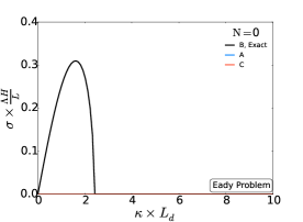
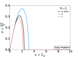
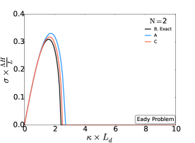
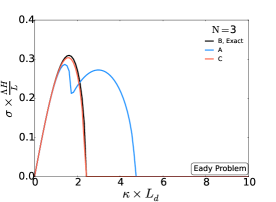
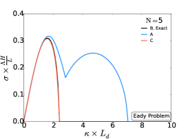
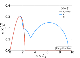
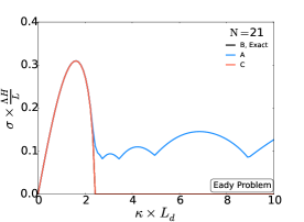
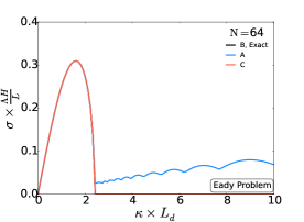
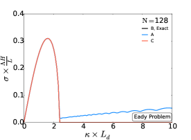
Figure 2: Growth rate for the Eady problem as a function of the zonal wavenumber ($l=0$) using approximations A, B (exact), C with various number of baroclinic modes ($\mathrm{N}$).

While the surface fields $\vartheta^{\pm}$ are dynamically passive in approximation A, the Eady problem can still be considered because the base-state PV defined via (40) converges to $\delta$-distributions on the boundaries (Section 3).

The base-state velocity in Approximation A is given by the series (34) and is a good approximation to the exact base-state velocity (33). But, according to approximation A, there is a nonzero interior base-state PV gradient given by the series (36). As $\mathrm{N}\to\infty$ the PV gradient in (36) converges in a distributional sense to Brethertonian sheets at $z=0$ and $-1$. But for numerical implementation of approximation A we stop short of $\mathrm{N}=\infty$. While the PV gradient is much larger at the boundaries, there is always interior structure in the PV (Figure 1c). We show that this spurious interior PV gradient has a strong and unpleasant effect on the approximate solution of the Eady stability problem.

To solve the Eady linear stability we linearize the interior equations (41) about the base-state velocity in (34) and the PV gradient in (36). We assume ${\breve{q}}_{k}=\hat{q}_{k}\exp[{{\rm i}(k\,x+l\,y-\omega^{A}\,t)}]$, etc, to obtain a $(\mathrm{N}+1)\times(\mathrm{N}+1)$ eigenproblem

$$\sum_{m=0}^{\mathrm{N}}\sum_{s=0}^{\mathrm{N}}\Xi_{nms}\Big{[}\breve{U}_{m}\,\hat{q}_{s}+\partial_{y}\,\breve{Q}_{s}\,\hat{\psi}_{m}\Big{]}=c^{A}\hat{q}_{n},$$ (64)

where $\breve{Q}_{s}$ are the coefficients of the series (36) and $c^{A}\stackrel{{\scriptstyle\mathrm{def}}}{{=}}\omega^{A}/k$. The eigenproblem (64) can be recast in the matrix form $\mathsf{A}\mathsf{q}=c^{A}\mathsf{q}$, where $\tilde{\mathsf{q}}=[\hat{q}_{0},\hat{q}_{1},\ldots,\hat{q}_{\mathrm{N}-1},\hat{q}_{\mathrm{N}}]^{\mathsf{T}}$ (Appendix B) and solved with standard methods.

Figure 2 shows the growth rate of the Eady instability according to approximation A, and compares this with the exact Eady growth rate. Approximation A does not do well, especially at large wavenumbers. The exact Eady growth rate has a high-wavenumber cut-off. At moderate values of $\mathrm{N}$, such as $3$, $5$ and $7$ approximation A produces unstable “bubbles” of instability at wavenumbers greater than the high-wavenumber cut-off. The growth rates in these bubbles are comparable to the true maximum growth rate. As $\mathrm{N}$ increases, the unstable bubbles are replaced by a long tail of unstable modes with a growth rate that slowly increases with $\kappa$. These spurious high-wavenumber instabilities are due to the rapidly oscillatory interior PV gradient which supports unphysical critical layers: see Figure 3.

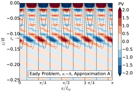
Figure 3: Structure of $\kappa=8$ unstable mode for the Eady problem obtained using approximation A and $\mathrm{N}=64$. Streamfunction is the black curves and PV is the colors. The streamfunction slightly tilts westward as $z$ increases. One can see the unphysical critical layer associated with the fast-oscillating base-state PV. The critical level, $z_{c}$, is the depth where the unstable wave speed matches the velocity of the base-state. Only the top quarter of the domain is shown.

5.2 Approximation B, the exact solution

In approximation B, the zero PV in the Eady problem implies $\breve{q}_{n}=\breve{\phi}_{n}=0$. The $\mathrm{N}+1$ modal equations (with $\beta=0$) are trivially satisfied; there is no interior contribution $(\phi^{B}_{\mathrm{N}}=0)$. Thus approximation B solves the Eady problem exactly.

Assuming $\sigma=\hat{\sigma}(z)\exp[{\rm i}(k\,x+l\,y-\omega^{B}\,t)]$, we obtain the solution to the surface streamfunction inversion problem (47)-(48)

$$\hat{\sigma}(z)=\frac{\cosh[\kappa(z+1)]}{\kappa\sinh\kappa}\,\vartheta^{\mathrm{+}}-\frac{\cosh(\kappa z)}{\kappa\sinh\kappa}\,\vartheta^{\mathrm{-}}\,,$$ (65)

where the magnitude of the wavenumber vector is $\kappa=\sqrt{k^{2}+l^{2}}$. We evaluate the surface streamfunction (65) at the boundaries to find the relationship between the streamfunction at the surfaces $\hat{\sigma}^{\pm}$ and the boundary fields $\vartheta^{\pm}$:

$$\begin{bmatrix}\hat{\sigma}^{+}\\ \hat{\sigma}^{-}\end{bmatrix}=\frac{1}{\kappa}\begin{bmatrix}\coth\kappa&-\text{csch}\,\kappa\\ \text{csch}\,\kappa&-\coth\kappa\end{bmatrix}\begin{bmatrix}{\hat{\vartheta}}^{\mathrm{+}}\\ {\hat{\vartheta}}^{\mathrm{-}}\end{bmatrix},$$ (66)

The nondimensional linearized boundary conditions (57) are

$${\hat{\vartheta}}^{\mathrm{+}}-\hat{\psi}^{+}=c^{B}{\hat{\vartheta}}^{\mathrm{+}}\,,\qquad\text{and}\qquad-\hat{\psi}^{-}=c^{B}{\hat{\vartheta}}^{\mathrm{-}}\,,$$ (67)

where $c^{B}=\omega^{B}/k$. Using the boundary conditions (67) in (66) we obtain an eigenvalue problem

$$\underbrace{\frac{1}{\kappa}\begin{bmatrix}\kappa-\coth\kappa&\text{csch}\,\kappa\\ -\text{csch}\,\kappa&\coth\kappa\\ \end{bmatrix}}_{\stackrel{{\scriptstyle\mathrm{def}}}{{=}}\mathsf{B}}\begin{bmatrix}{\hat{\vartheta}}^{\mathrm{+}}\\ {\hat{\vartheta}}^{\mathrm{-}}\end{bmatrix}=c^{B}\begin{bmatrix}{\hat{\vartheta}}^{\mathrm{+}}\\ {\hat{\vartheta}}^{\mathrm{-}}\end{bmatrix}\,.$$ (68)

The eigenvalues of $\mathsf{B}$ are given by the celebrated dispersion relation for the Eady problem (Pedlosky 1987; Vallis 2006)

$$c^{B}=\tfrac{1}{2}\pm\tfrac{1}{\kappa}\Big{[}\Big{(}\tfrac{\kappa}{2}-\tanh\tfrac{\kappa}{2}\Big{)}\Big{(}\tfrac{\kappa}{2}-\coth\tfrac{\kappa}{2}\Big{)}\Big{]}^{1/2}\,.$$ (69)

5.3 Approximation C

Approximation C expands both the streamfunction and the PV in standard vertical modes. Thus in the Eady problem the PV is exactly zero, as it should be: $q=\breve{q}_{n}=0$. (This contrasts with approximation A, in which the differentiation of the truncated series approximation to the streamfunction induces an unphysical oscillatory base-state PV gradient.) Thus approximation C does not have the spurious critical layers that bedevil A. Moreover, in approximation C, the $\mathrm{N}+1$ modal equations (with $\beta=0$) in (59) are trivially satisfied, and the inversion relationship (60) provides a simple connection between the streamfunction and the fields $\vartheta^{\pm}$. The base velocity for the Eady problem in approximation C is the series in (34) (the same as A). From the exact shear at the boundaries we obtain the exact base-state boundary variables

$${\varTheta^{\pm}}=-y\,.$$ (70)

We linearize the boundary equations (61) about the base-state (36) and (70), to obtain

$$\partial_{t}\vartheta^{\pm}+{U^{\mathrm{G}}_{\mathrm{N}}}^{\pm}\partial_{x}\vartheta^{\pm}-\,\sum_{k=0}^{\mathrm{N}}\partial_{x}\breve{\psi}_{k}\mathsf{p}_{k}^{\pm}=0\,.$$ (71)

Assuming $\vartheta^{\pm}={\hat{\vartheta}}^{\pm}\exp[{\rm i}(k\,x+l\,y-\omega^{C}\,t)]$, and using the inversion relationship (60), we obtain a $2\times 2$ eigenproblem

$$\mathsf{C}\,\begin{bmatrix}{\hat{\vartheta}}^{\mathrm{+}}\\ {\hat{\vartheta}}^{\mathrm{-}}\end{bmatrix}=c^{C}\,\begin{bmatrix}{\hat{\vartheta}}^{\mathrm{+}}\\ {\hat{\vartheta}}^{\mathrm{-}}\end{bmatrix}\,,$$ (72)

where matrix $\mathsf{C}$ is defined in appendix C. It is straightforward to show that $c^{C}$ converges to the exact eigenspeed. i.e., $c^{C}\to c^{B}$ as $\mathrm{N}\to\infty$ (Appendix B). Figure 2 shows that approximation C successfully captures the structure of the Eady growth rate even with modest values of $\mathrm{N}$.

5.4 Remarks on convergence

The crudest truncation (i.e. $\mathrm{N}=0$) is stable for both approximations A and C (Figure 2). With one baroclinic mode ($\mathrm{N}=1$) the growth rates $\left(\omega_{i}=k\times\mathrm{Im}\{c\}\right)$ are qualitatively consistent with the exact solution, and the results improve with $\mathrm{N}=2$. With a moderate number of baroclinic modes modes ($\mathrm{N}>2$) approximations A and C converge rapidly to the exact growth rate at wavenumbers less than about $2.2$ — see figure 2. But surprisingly the convergence of the growth rate at the most unstable mode ($\kappa\approx 1.6$) is faster in approximation A ($\sim\!\mathrm{N}^{-4}$) than in approximation C ($\sim\!\mathrm{N}^{-2}$) — see figure 4. However, the convergence in approximation C is uniform: there are no spurious high-wavenumber instabilities.

Figure 4 also shows that the approximation A convergence of the growth rate to zero at $\kappa=8$ is slow ($\sim\!\mathrm{N}^{-1}$). While the growth rate does converge to zero at a fixed wavenumber, such as $\kappa=8$, we conjecture that there are always faster growing modes at larger wavenumbers.

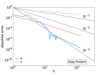
Figure 4: Absolute error as a function of number of baroclinic modes ($\mathrm{N}$) for the growth rates of the Eady problem. The solid lines show the error at the exact fastest growing mode ($\kappa\approx 1.6$). The dashed line is the approximation A error at $\kappa=8$.

6 The Green problem

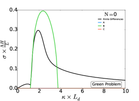
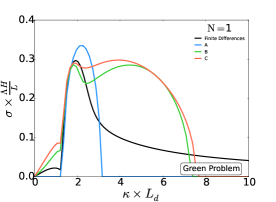
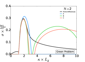
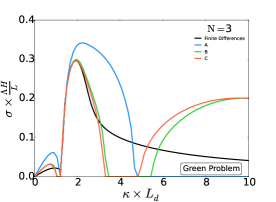
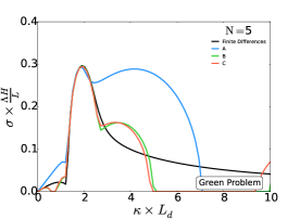
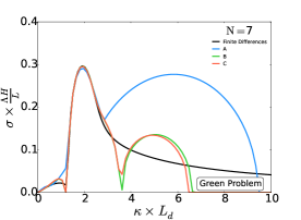
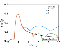
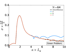
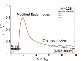
Figure 5: Growth rate for the Green problem with $\hat{\beta}=1$ as a function of the zonal wavenumber ($l=0$) using approximations A, B, C with various number of baroclinic modes ($\mathrm{N}$). The black line is a finite-differences solution with 1000 vertical levels.

To further explore the relative merit and efficiency of approximations A, B, and C we study the instability properties of a system with nonzero $\beta$. For simplicity, we consider a problem with Eady’s base-state $\psi=-(1+z)y$ on a $\beta$-plane. This is similar to the problem originally considered by Green (1960) and Charney (1971). The major difference is that Charney considered a vertically semi-infinite domain (Charney 1947; Pedlosky 1987) while we follow Green and consider a finite-depth domain with $-1<z<0$.

We obtain the exact system for this “Green problem” by linearizing the QG equations (6)-(9) about the base-state (33) with background PV $\beta y$, where $\hat{\beta}$ is the nondimensional planetary PV gradient. Assuming $\psi=\hat{\phi}\exp[{\rm i}(k\,x+l\,y-\omega\,t)]$, we obtain

$$(U-c)\left[\hat{\phi}_{zz}-\kappa^{2}\hat{\phi}\right]+\hat{\beta}\hat{\phi}=0\,,\qquad-1<z<0\,,$$ (73)

and

$$(U-c)\,\hat{\phi}_{z}-\hat{\phi}=0\,,\qquad z=-1\,,0\,.$$ (74)

As a reference solution, we solve the eigenproblem (73)-(74) using a centered second-order finite-difference scheme with 1000 vertical levels: see Figure 5.

The Green problem supports three classes of unstable modes, indicated in the lower right panel ($\mathrm{N}=128$) of Figure 5: $(1)$ the “modified Eady modes”, which are instabilities that arise from the interaction of Eady-like edge waves, only slightly modified by $\beta$; $(2)$ the “Green modes”, which are very long slowly growing modes (Vallis 2006); (3) the high-wavenumber “Charney modes” are critical layer instabilities that arise from the interaction of the surface edge wave with the interior Rossby wave that is supported by nonzero $\beta$.

6.1 Implementation of approximation A

The base-state for the Green problem is the same as in the Eady problem. In approximation A, the $\beta$-term adds only a diagonal term to the Eady system (64) (see appendix C).

6.2 Implementation of approximation B

The base-state is the same as in Eady problem. The steady streamfunction and buoyancy fields that satisfy (56) and (57) exactly are

$$\Sigma=-\left(1+z\right)y\qquad\text{and}\qquad\Theta^{\pm}=-y\,.$$ (75)

Assuming $\breve{q}_{n}=\hat{q}_{n}(z)\exp[{\rm i}(k\,x+l\,y-\omega^{B}\,t)]$, the $\mathrm{N}+1$ interior equations (56) linearized about (75) become

$$\sum_{s=0}^{\mathrm{N}}\xi_{ns}\hat{q}_{s}+\hat{\beta}\left(\hat{\phi}_{n}+\hat{\sigma}_{n}\right)=c^{B}_{c}\,\hat{q}_{n}\,,$$ (76)

where

$$\xi_{ns}\stackrel{{\scriptstyle\mathrm{def}}}{{=}}\tfrac{1}{h}\int_{z^{-}}^{z^{+}}\!\!\!\!\!\mathsf{p}_{n}\,\mathsf{p}_{s}\,\left(z+1\right){\rm d}z\,.$$ (77)

The boundary conditions (57), linearized about (75), become

$$\hat{\vartheta}^{+}-\sum_{s=0}^{\mathrm{N}}\mathsf{p}_{s}^{+}\hat{\phi}_{s}-\hat{\sigma}^{+}=c^{B}_{c}\,\hat{\vartheta}^{+}\,,$$ (78)

and

$$-\sum_{s=0}^{\mathrm{N}}\mathsf{p}_{s}^{-}\hat{\phi}_{s}-\hat{\sigma}^{-}=c^{B}_{c}\,\hat{\vartheta}^{-}\,,$$ (79)

where $\hat{\sigma}$ is given by (65). We use the inversion relationship (55) and the Neumann-to-Dirichlet map (66) to recast this eigenproblem into standard form $\mathsf{B}\,\tilde{\mathsf{q}}=c^{B}\,\tilde{\mathsf{q}}$, where $\tilde{\mathsf{q}}=[\hat{\vartheta^{\mathrm{+}}},\hat{q}_{0},\hat{q}_{1},\ldots,\hat{q}_{\mathrm{N}-1},\hat{q}_{\mathrm{N}},\hat{\vartheta^{\mathrm{-}}}]^{\mathsf{T}}$ (see appendix C).

6.3 Implementation of approximation C

Again the base-state is the same as in the Eady problem. But now there are $\mathrm{N}+3$ equations: the two boundary equations of Eady’s problem (71) plus $\mathrm{N}+1$ interior equations

$$\sum_{m=0}^{\mathrm{N}}\sum_{s=0}^{\mathrm{N}}\Xi_{nms}\breve{U}_{m}\,\hat{q}_{s}+\hat{\beta}\hat{\psi}_{n}=c^{C}\hat{q}_{n}\,,$$ (80)

We use the inversion relationship (60) in (80) to recast this eigenproblem in the form $\mathsf{C}\,\tilde{\mathsf{q}}=c^{C}\tilde{\mathsf{q}}$, where $\tilde{\mathsf{q}}$ is defined as in approximation B (see appendix C).

6.4 Remarks on convergence

The most crude truncation ($\mathrm{N}=0$) is stable for approximations A and C. In contrast, the $\mathrm{N}=0$ truncation in approximation B is qualitatively consistent with the modified Eady instabilities: see figure 5. With a moderate number of baroclinic modes ($\mathrm{N}=2$ or $3$), approximations A, B and C all resolve the modified Eady modes relatively well. At the most unstable modified Eady mode ($\kappa\approx 1.9$), approximation B has typically the smallest error because it solves the surface problem exactly. As in the Eady problem, approximation A converges ($\sim\mathrm{N}^{-4}$) faster than approximations B and C ($\sim\mathrm{N}^{-2}$) at the most unstable mode, but B and C converge faster at high wavenumbers (6).

Approximations A, B, and C all converge very slowly to the high-wavenumber Charney modes (Figures 5 and 6). These modes are interior critical-layer instabilities (Pedlosky 1987) and the critical layer is confined to a small region about the steering level (i.e., the depth at which the phase speed matches the base velocity — see figure 7). With finite base-state shear, the critical layer is always in the interior. Thus, the problem is not that standard vertical modes are inefficient because they do not satisfy inhomogeneous boundary conditions; a low resolution finite-difference solution also presents such “bubbles” in high-wavenumber growth rates (not shown). Resolution of the interior critical layer, not the surface boundary condition, is a problem for all methods at high wavenumbers. The “surface-aware” modes of Smith and Vanneste (2013) have the same limitation — a large number of vertical modes is required to resolve the critical-layer instabilities (K. S. Smith, pers. comm.).

For example, with $\mathrm{N}<25$, at $\kappa=8$, approximations are qualitatively inconsistent with the high-resolution finite-difference solution. For larger values of $\mathrm{N}$, the growth rate convergence for approximations B and C scales $\sim\!\mathrm{N}^{-3}$. The growth rate for approximation A converges painfully slowly ($\sim\!\mathrm{N}^{-1}$). As in the Eady problem, at large wavenumbers, the growth rate for approximation A is qualitatively different from that of the finite-difference solution because of spurious instabilities associated with the rapidly oscillatory base-state PV gradient.

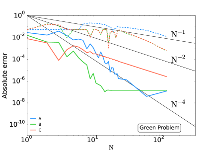
Figure 6: Absolute error as a function of number of baroclinic modes ($\mathrm{N}$) for the growth rates of the Green problem. The solid line represent the error at the exact fastest growing mode ($\kappa\approx 1.9$). The dashed line is the error at $\kappa=8$.

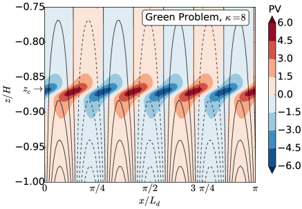
Figure 7: Wave structure of the $\kappa=8$ unstable mode for the Green problem with $\hat{\beta}=1$ solved using a second-order finite-difference scheme with 1000 vertical levels. Streamfunction (black contours) and potential vorticity (colors). The streamfunction slightly tilts westward as $z$ increases. The potential vorticity is confined to a small region, the critical layer. The critical level, $z_{c}$, is the depth where the unstable wave speed matches the velocity of the base-state. Only the bottom quarter of the domain is shown.

7 Summary and conclusions

The Galerkin approximations A, B, and C are equivalent if there is are no buoyancy variations at the surfaces. Thus all three approximations are well-suited for applications with zero surface buoyancy (Flierl 1978; Fu and Flierl 1980; Hua and Haidvogel 1986). But with nonzero surface buoyancy the three approximations are fundamentally different.

Approximation A, originally introduced by Flierl (1978), represents the streamfunction as a Galerkin series in standard vertical modes and defines the potential vorticity so that the inversion problem is satisfied exactly. The most important limitation of A is that the interior PV evolves independently of the surface buoyancy (as if $\vartheta^{\pm}$ were zero). The evolution equations in approximation A (41) are relatively simple, and the system conserves energy (44) and potential enstrophy (45). But, in approximation A, nonzero surface buoyancy results in an interior PV that distributionally converges to $\delta$-distributions at the boundaries as $\mathrm{N}\to\infty$. These smeared-out Brethertonian $\delta$-functions provide a very inaccurate representation of the true inhomogeneous surface boundary condition. Finite difference schemes have a similar pathology (Smith 2007; Tulloch and Smith 2009a). As a result of this artificial interior PV gradient, solutions with a small number of modes are qualitatively misleading and convergence at large wavenumbers is very slow ($\sim\!\mathrm{N}^{-1}$). Slow convergence was previously noted by Hua and Haidvogel (1986) — see their figure 2. Furthermore, even if heroic values of $\mathrm{N}$ achieve convergence at say $\kappa=10$, we conjecture that there will always be spurious unstable modes at even larger wavenumbers. In some simulations these unphysical high-wavenumber instabilities might be eliminated by hyperviscosity or by a scale-selective filter. But one must be aware of potential effects on the evolution of the system.

Approximation B, originally introduced by Tulloch and Smith (2009b) using one baroclinic mode and constant buoyancy frequency, takes the opposite starting point from approximation A. B represents the PV as a Galerkin series in standard modes and calculates the streamfunction that satisfies the exact inversion problem associated with the approximate PV. The linear inversion problem can be split into an interior contribution with homogeneous boundary conditions and a surface contribution with zero interior source and inhomogeneous boundary conditions (Lapeyre and Klein 2006; Tulloch and Smith 2009b). Thus the exact interior streamfunction associated with the approximate PV is a Galerkin series, but the surface streamfunction must be computed using other methods. Because the surface streamfunction projects onto the interior solution the energy is not diagonalized. Indeed, approximation B conserves neither energy nor potential enstrophy if $\beta\neq 0$.

Approximation C represents both the PV and the streamfunction by Galerkin series. Although the inversion problem is not satisfied exactly, the relation between modal streamfunction $\breve{\psi}_{n}$ and PV $\breve{q}_{n}$ is obtained by Galerkin projection of the exact inversion relationship and prominently exhibits the surface buoyancy fields: see (60). Approximation C is the most consistent because it uses the same level of approximation for both PV and streamfunction. The evolution equations (59) are relatively simple, and the approximate system conserves total energy (62). The most vexing limitation of C is the lack of potential enstrophy conservation with $\beta\neq 0$. But this does not mean that approximation A is better than approximation C: all approximations conserve potential enstrophy when $\beta=0$, or if $\vartheta^{\pm}=0$, and none conserve an analog of the exact potential enstrophy (45) when $\beta\neq 0$ and $\vartheta^{\pm}\neq 0$.

With nonzero interior PV gradients the convergence of all approximations is slow for the high-wavenumber Charney-type modes. The critical layer associated with these modes spans a very small fraction of the total depth (Figure 7). To accurately resolve these near-singularities at the steering level there is no better solution than having high vertical resolution in the interior.

For problems with nonuniform surface buoyancy and nonzero interior PV gradient, we recommend approximation C for obtaining solutions to the three-dimensional QG equations using standard vertical modes.

The codes that produced the numerical results of this paper, plotting scripts, and supplementary figures are openly available at github.com/crocha700/qg$\_$vertical$\_$modes.

$$\frac{{\rm d}^{2}\mathsf{P}_{n}}{{\rm d}Z^{2}}+\left[\rho^{2}_{n}-\Lambda(Z)\right]\mathsf{P}_{n}=0\,,$$ (81)

defined on the interval $Z\in[0,\pi]$ with boundary conditions

$$\mathsf{P}_{n}^{\prime}(0)-\gamma_{0}\mathsf{P}_{n}(0)=0\,,\;\;\text{and}\;\;\mathsf{P}^{\prime}_{n}(\pi)-\gamma_{\pi}\mathsf{P}_{n}(\pi)=0$$ (82)

where $\gamma_{0}$ and $\gamma_{\pi}$ are real constants of arbitrary sign and $\rho_{n}^{2}$ is the eigenvalue. The equations defining the standard modes (1)-(2) can be brought to this form using the following Liouville transformation

$$Z(z)=\frac{1}{\bar{Z}}\int_{z^{-}}^{z}S(\xi)^{-1/2}{\rm d}\xi\,,\;\;\text{with}\;\;\bar{Z}\stackrel{{\scriptstyle\mathrm{def}}}{{=}}\frac{1}{\pi}\int_{z^{-}}^{z^{+}}S(\xi)^{-1/2}{\rm d}\xi\,,$$ (83)

and

$$\mathsf{P}_{n}(Z)=S(z)^{1/4}\mathsf{p}_{n}(z)\,,\quad\text{where}\quad S(z)\stackrel{{\scriptstyle\mathrm{def}}}{{=}}\frac{f_{0}^{2}}{N^{2}(z)}\,.$$ (84)

The eigenvalues are related by $\rho_{n}=\bar{Z}\kappa_{n}$ and

$$\Lambda(Z)=\bar{Z}^{2}\left[\frac{1}{4}\frac{{\rm d}^{2}S}{{\rm d}z^{2}}-\frac{1}{16S}\left(\frac{{\rm d}S}{{\rm d}z}\right)^{2}\right]\,.$$ (85)

The boundary condition for the standard modes (2) implies that the transformed modes satisfy (82) with

$$\gamma_{0}=\frac{4S(z^{-})^{1/2}}{\bar{Z}{\rm d}S(z^{-})/{\rm d}z}\,,\quad\text{and}\quad\gamma_{\pi}=-\frac{4S(z^{+})^{1/2}}{\bar{Z}{\rm d}S(z^{+})/{\rm d}z}\,.$$ (86)

If ${\rm d}S/{\rm d}z=0$ at a boundary then the appropriate condition at that boundary is $P_{n}=0$.

A special case of Theorem I from Jackson (1914) states that the expansion of a function $\phi(Z)$ as a series in eigenfunctions $\mathsf{P}_{n}$ converges absolutely and uniformly provided that both ${\rm d}\phi/{\rm d}Z$ and ${\rm d}\Lambda/{\rm d}Z$ are continuous and bounded, regardless of whether or not $\phi$ satisfies the same boundary conditions as $\mathsf{P}_{n}$. (The remainder of the theorem concerns the rate of convergence under stronger conditions on $\phi$ and $\Lambda$.) The streamfunction, potential vorticity, and buoyancy frequency profiles are typically assumed to be smooth in studies of QG dynamics, which implies that both $\phi$ and $\lambda$ will satisfy the above conditions. Uniform convergence over $Z\in[0,\pi]$ implies uniform convergence over $z\in[z^{-},z^{+}]$.

[B] Details of the derivation of quadratic conservation laws for approximate equations

.1 Approximation A

To obtain the energy conservation in approximation A we multiply the modal equations (41) by $-\breve{\psi}_{n}$, integrate over the horizontal surface, and sum of on n, to obtain

$$\frac{{\rm d}}{{\rm d}t}\sum_{n=0}^{\mathrm{N}}\int\tfrac{1}{2}\left[(\nabla\breve{\psi_{n}})^{2}+\kappa_{n}^{2}\breve{\psi}_{n}^{2}\right]{\rm d}S\,+$$

$$\sum_{n=0}^{\mathrm{N}}\sum_{m=0}^{\mathrm{N}}\sum_{s=0}^{\mathrm{N}}\Xi_{nms}\int\,\breve{\psi}_{n}\,\mathsf{J}\left(\breve{\psi}_{m},\triangle_{s}\breve{\psi}_{s}\right){\rm d}S=0\,.$$ (87)

Notice that

$$\int\breve{\psi}_{n}\,\mathsf{J}\left(\breve{\psi}_{m},\triangle_{s}\breve{\psi}_{s}\right)\,{\rm d}S=\int\triangle_{s}\breve{\psi}_{s}\,\mathsf{J}\left(\breve{\psi}_{n},\breve{\psi}_{m}\right)\,{\rm d}S\,.$$ (88)

Hence the triple sum term in .1 vanishes identically because $\Xi_{nms}$ is fully symmetric and the Jacobian is skew-symmetric. Thus we obtain conservation of energy (44). Similarly, to obtain the potential enstrophy conservation law in (45) we multiply the modal equations (41) by $\triangle_{n}\breve{\psi}_{n}$, integrate over the surface, sum on $n$, and invoke the same symmetry arguments used for the energy conservation.

.2 Approximation B

Energy nonconservation

The analog of (11) in approximation B is

$$E^{B}_{N}\stackrel{{\scriptstyle\mathrm{def}}}{{=}}E_{\phi}+E_{\sigma}+E_{\phi\sigma}\,.$$ (89)

The three terms in (89) are

$$E_{\phi} =\tfrac{1}{h}\int\left[\left|\nabla\phi^{B}_{\mathrm{N}}\right|^{2}+\left(\tfrac{f_{0}}{N}\right)^{2}\left(\partial_{z}\phi^{B}_{\mathrm{N}}\right)^{2}\right]{\rm d}V$$

$$=\sum_{n=0}^{\mathrm{N}}\,\int\tfrac{1}{2}\left[\left|\nabla\breve{\phi}_{n}\right|^{2}+\kappa_{n}^{2}\breve{\phi}_{n}^{2}\right]\,{\rm d}S\,,$$ (90)

$$E_{\sigma}=\tfrac{1}{h}\int\tfrac{1}{2}\left[\left|\nabla\sigma\right|^{2}+\left(\tfrac{f_{0}}{N}\right)^{2}\left(\partial_{z}\sigma\right)^{2}\right]{\rm d}V,$$ (91)

and

$$E_{\phi\sigma} =\tfrac{1}{h}\int{}\left[\nabla\phi^{B}_{\mathrm{N}}\bm{\cdot}\nabla\sigma+\left(\tfrac{f_{0}}{N}\right)^{2}\partial_{z}\phi^{B}_{\mathrm{N}}\,\partial_{z}\sigma\right]{\rm d}V,$$

$$=\sum_{n=0}^{\mathrm{N}}\int{}\breve{\sigma}_{n}\triangle_{n}\breve{\phi}_{n}\,{\rm d}S\,.$$ (92)

The cross-term $E_{\phi\sigma}$ is not zero because the surface streamfunction $\sigma$ projects on the standard vertical modes i.e., $\breve{\sigma}_{n}$ is nonzero. To obtain an equation for $E_{B}$ we form evolution equations for the three components in (89) and add them. The final result is

$$\frac{{\rm d}E^{B}_{N}}{{\rm d}t} =\sum_{n=0}^{\mathrm{N}}\sum_{s=0}^{\mathrm{N}}\tfrac{1}{h}\int\!\!\mathsf{p}_{n}\mathsf{p}_{s}(\breve{\phi}_{n}+\breve{\sigma}_{n})\mathsf{J}(\sigma,\breve{q}_{s}){\rm d}V$$

$$+\sum_{m=0}^{\mathrm{N}}\sum_{n=0}^{\mathrm{N}}\sum_{s=0}^{\mathrm{N}}\Xi_{mns}\int\ \breve{\sigma}_{n}\mathsf{J}(\breve{\phi}_{m},\triangle_{s}\breve{\phi}_{s})\,{\rm d}S\,.$$ (93)

The simplest model with barotropic interior dynamics ($\mathrm{N}=0$) conserves energy. With richer interior structure, however, the right-hand-side of (.2) is generally nonzero. Consider the “two surfaces and two modes” (TMTS) model of Tulloch and Smith (2009b), corresponding to $\mathrm{N}=1$ with constant buoyancy frequency. Using nondimensional variables the energy equation (.2) becomes

$$\frac{{\rm d}E^{B}_{1}}{{\rm d}t}=\int\left[\phi_{1}\,\mathsf{J}\left(\breve{\sigma}_{1}\,,\triangle_{1}\breve{\phi}_{1}\right)-\tfrac{1}{\sqrt{2}}\triangle_{1}\breve{\phi}_{1}\,\mathsf{J}\left(\breve{\sigma}_{1}\,,\breve{\sigma}_{2}\right)\right]{\rm d}S\,.$$ (94)

We now construct an example in which we can analytically show that the right-hand-side of (94) is nonzero. This example should be interpret as an initial condition for which energy is guaranteed to grow or decay. For simplicity we consider $\triangle\breve{\phi}_{1}=\lambda\breve{\phi}_{1}$, where $\lambda$ is a constant, so that the first term on the right-hand-side of (94) is identically zero. As for the surface streamfunction, we choose

$$\sigma=\frac{\cosh{(z+1)}}{\sinh 1}\cos x+\frac{\cosh{z}}{\sinh 1}\sin x\,.$$ (95)

We use $\phi_{1}=\sin x\,\cos y$ so that all fields are periodic with the same period. Integrating over one period in both directions gives

$$\frac{{\rm d}E^{B}_{1}}{{\rm d}t}=\frac{\lambda}{\sqrt{2}\,(1+5\pi^{2}+4\pi^{4})}\neq 0\,.$$ (96)

The total energy $E^{B}_{1}$ grows or decays depending on the sign of $\lambda$. Thus the analog of the exact energy (11) is not generally conserved in approximation B.

potential enstrophy nonconservation

The analog of the exact potential enstrophy (15) is not conserved in approximation B. We attempt to form a potential enstrophy conservation by multiplying the interior equations (56) by $\triangle_{n}\breve{\phi}_{n}$ and integrating over the surface, and summing on $n$,

$$\frac{{\rm d}}{{\rm d}t}\sum_{n=0}^{\mathrm{N}}\int\tfrac{1}{2}(\triangle_{n}\breve{\phi}_{n})^{2}{\rm d}S-\beta\sum_{n=0}^{\mathrm{N}}\int\triangle_{n}\breve{\sigma}_{n}\partial_{x}\breve{\phi}_{n}{\rm d}S=0\,.$$ (97)

The potential enstrophy given by the sum on the left-hand-side of (97) is conserved in the special case $\beta=0$. For $\beta\neq 0$ we first form an equation for $\triangle_{n}\breve{\sigma}_{n}$, and then cross-multiply with the modal equations (56), integrate over the surface, and sum on $n$. Eliminating the $\beta$-term in (97) yields

$$\frac{{\rm d}}{{\rm d}t} \sum_{n=0}^{\mathrm{N}}\tfrac{1}{2}(\triangle_{n}\breve{\phi}_{n})^{2}+(\triangle_{n}\breve{\sigma}_{n})\breve{q}_{n}{\rm d}S=$$

$$-\sum_{m=0}^{\mathrm{N}}\sum_{n=0}^{\mathrm{N}}\sum_{s=0}^{\mathrm{N}}\Xi_{mns}\int\triangle_{n}\breve{\sigma}_{n}\mathsf{J}\left(\breve{\phi}_{m}\,,\triangle_{s}\breve{\phi}_{s}\right){\rm d}S$$

$$-\sum_{n=0}^{\mathrm{N}}\tfrac{1}{h}\int\triangle_{n}\breve{\sigma}_{n}\mathsf{p}_{n}\mathsf{p}_{n}\mathsf{J}\left(\sigma\,,\triangle_{s}\breve{\phi}_{s}\right){\rm d}V$$

$$+\sum_{n=0}^{\mathrm{N}}\sum_{m=0}^{\mathrm{N}}\tfrac{1}{h}\int\triangle_{n}\breve{\phi}_{n}\,\Big{[}\mathsf{p}_{n}^{+}\mathsf{J}\left(\sigma^{+}+\mathsf{p}_{m}^{+}\breve{\phi}_{m}\,,\vartheta^{\mathrm{+}}\right)$$

$$~{}~{}~{}~{}~{}~{}~{}~{}~{}~{}~{}~{}~{}~{}~{}~{}~{}~{}~{}~{}~{}~{}~{}~{}~{}~{}~{}~{}-\mathsf{p}_{n}^{-}\mathsf{J}\left(\sigma^{-}+\mathsf{p}_{m}^{-}\breve{\phi}_{m}\,,\vartheta^{\mathrm{-}}\right)\Big{]}{\rm d}S\,.$$ (98)

The right-hand-side of (.2) is nonzero even in the simplest model ($\mathrm{N}=0$).

.3 Approximation C

To obtain the conservation of energy in approximation C we multiply the modal equations (59) by $-\breve{\psi}_{n}$, integrate over the horizontal surface, and sum on $n$, to obtain

$$\frac{{\rm d}}{{\rm d}t} \sum_{n=0}^{\mathrm{N}}\int\left[(\nabla\breve{\psi}_{n})^{2}+\kappa_{n}^{2}\breve{\psi}_{n}^{2}\right]{\rm d}S\,$$

$$-\sum_{n=0}^{\mathrm{N}}\tfrac{1}{h}\int\breve{\psi}_{n}\partial_{t}\,(\mathsf{p}^{+}_{n}\vartheta^{\mathrm{+}}-\mathsf{p}^{-}_{n}\vartheta^{\mathrm{-}})\,{\rm d}S\,$$

$$+\sum_{n=0}^{\mathrm{N}}\sum_{m=0}^{\mathrm{N}}\sum_{s=0}^{\mathrm{N}}\Xi_{nms}\int{}\breve{\psi}_{n}\,\mathsf{J}\left(\breve{\psi}_{m},\triangle_{s}\breve{\psi}_{s}\right)\,{\rm d}S=0\,,$$ (99)

The triple sum term vanishes by the same symmetry arguments used above in approximation A. The term on the second line of (.3) is also zero: multiply the boundary conditions (61) by $\mathsf{p}_{n}^{\pm}\,\breve{\psi}_{n}$ and integrate over the horizontal surface. Thus we obtain the energy conservation law in (62).

Potential enstrophy nonconservation

As in approximation B, the analog of the exact potential enstrophy (15) is not conserved in approximation C. The potential enstrophy equation with $\beta\neq 0$ is formed analogously to the approach used above in approximation B. The final result is

$$\frac{{\rm d}}{{\rm d}t}\sum_{n=0}^{\mathrm{N}}\int\frac{\breve{q}_{n}^{2}}{2}+\breve{q}_{n}\triangle_{n}\breve{\sigma}_{n}\,{\rm d}S=$$

$$+\sum_{m=0}^{\mathrm{N}}\sum_{n=0}^{\mathrm{N}}\tfrac{1}{h}\int\!\!\breve{q}_{n}\mathsf{p}_{n}^{+}\mathsf{p}_{m}^{+}\mathsf{J}\left(\breve{\psi}_{m},\vartheta^{\mathrm{+}}\right)-\breve{q}_{n}\mathsf{p}_{n}^{-}\mathsf{p}_{m}^{-}\mathsf{J}\left(\breve{\psi}_{m},\vartheta^{\mathrm{-}}\right)$$

$$-\sum_{m=0}^{\mathrm{N}}\sum_{n=0}^{\mathrm{N}}\sum_{s=0}^{\mathrm{N}}\int\Xi_{mns}\triangle_{n}\breve{\sigma}_{n}\mathsf{J}\left(\breve{\psi}_{m}\,,\breve{q}_{s}\right)\,.$$ (100)

The right-hand-side of (.3) is zero for the simplest model ($\mathrm{N}=0$), but it is generally nonzero.

[C] Details of the stability problems

.4 The interaction tensor

Because the standard vertical modes with constant stratification are simple sinusoids (32), the interaction coefficients (42) can be computed analytically. First we recall that $\Xi_{ijk}$ is fully symmetric. Permuting the indices so that $i\geq j\geq k$ we obtain

$$\vspace{.1cm}\Xi_{ijk}=\begin{cases}\,\,\,\,1:&i=j,\,k=0\,;\\ \frac{\sqrt{2}}{2}:&i=j+k\,;\\ \vspace{.1cm}\,\,\,\,0:&\text{otherwise}\,.\end{cases}$$ (101)

The second line in (101) corrects a factor of $\tfrac{1}{2}$ missed by Hua and Haidvogel (1986).

.5 Approximation A

Using the symmetry in $\Xi_{nms}$, and the inversion relation (40), we rewrite row $n+1$ of the linear Green system

$$\sum_{s=0}^{\mathrm{N}}\sum_{m=0}^{\mathrm{N}}\Xi_{nms}\left(\breve{U}_{m}+\partial_{y}\breve{Q}_{m}\,\alpha_{s}\right)\hat{q}_{s}+\hat{\beta}\alpha_{n}\hat{q}_{n}=c^{A}\hat{q}_{n},$$ (102)

where the inverse of the $n$’th mode Helmholtz operator in Fourier space is

$$\alpha_{n}\stackrel{{\scriptstyle\mathrm{def}}}{{=}}-(\kappa^{2}+(n\pi)^{2})^{-1}\,.$$ (103)

The Eady problem is the special case $\hat{\beta}=0$. We use a standard eigenvalue-eigenvector algorithm to obtain the approximate eigenspeed $c^{A}$.

.6 Approximation B

The Green eigenvalue problem in (76) through (79) can be recast in the standard form $\mathsf{B}\,\mathsf{q}=c^{B}\,\mathsf{q}$, where $\tilde{\mathsf{q}}=[\hat{\vartheta^{\mathrm{+}}},\hat{q}_{0},\hat{q}_{1},\ldots,\hat{q}_{\mathrm{N}-1},\hat{q}_{\mathrm{N}},\hat{\vartheta^{\mathrm{-}}}]^{\mathsf{T}}$. The first and last rows of the system stem from the boundary conditions (78)-(79)

$$\left(1-\frac{\coth{\kappa}}{\kappa}\right)\!\hat{\vartheta}^{+}-\sum_{s=0}^{\mathrm{N}}\!\mathsf{p}_{s}^{+}\alpha_{s}\hat{q}_{s}-\frac{\text{csch}\,{\kappa}}{\kappa}\,\hat{\vartheta}^{-}=c^{B}\,\hat{\vartheta}^{+}\,,$$ (104)

and

$$\frac{\text{csch}\,{\kappa}}{\kappa}\,\hat{\vartheta}^{+}-\sum_{s=0}^{\mathrm{N}}\!\mathsf{p}_{s}^{-}\alpha_{s}\,\hat{q}_{s}+\frac{\coth{\kappa}}{\kappa}\,\hat{\vartheta}^{-}=c^{B}\,\hat{\vartheta}^{-}\,.$$ (105)

The $(n+1)$’th row originates from the $n$’th interior equation (76)

$$-\hat{\beta}\,\mathsf{p}_{n}^{+}\,\alpha_{n}\,\vartheta^{\mathrm{+}}+\sum_{s=0}^{\mathrm{N}}\gamma_{ns}\hat{q}_{s}+\left(\beta\alpha_{n}+1\right)+\hat{\beta}\,\mathsf{p}_{n}^{-}\,\alpha_{n}\,\vartheta^{\mathrm{-}}=c^{B}\,\hat{q}_{n}\,,$$ (106)

where the symmetric matrix $\gamma_{ms}$ is

$$\gamma_{ij}\stackrel{{\scriptstyle\mathrm{def}}}{{=}}\int_{-1}^{0}\mathsf{p}_{i}\,\mathsf{p}_{j}\,z\,{\rm d}z=\begin{cases}\vspace{.1cm}\,\,\,\,\,\,\,\,\,\,-\tfrac{1}{2}:&i=j\,;\\ \vspace{.1cm}\,\,\,\,\,\,\,\,\,\,\frac{2\sqrt{2}}{(j\,\pi)^{2}}:&i=0,\,j\,\,\text{ is odd}\,;\\ \tfrac{4\,\left(i^{2}+j^{2}\right)}{\left[\left(i^{2}-j^{2}\right)\,\pi\right]^{2}}:&\,\,i+j\,\text{ is odd}\,.\end{cases}$$ (107)

.7 Approximation C

The Eady problem

The $2\times 2$ eigenproblem is

$$\underbrace{\begin{bmatrix}{U^{\mathrm{G}}_{\mathrm{N}}}^{+}+\Sigma_{\mathrm{N}}&-\Omega_{\mathrm{N}}\\ \Omega_{\mathrm{N}}&{U^{\mathrm{G}}_{\mathrm{N}}}^{-}-\Sigma_{\mathrm{N}}\end{bmatrix}}_{\stackrel{{\scriptstyle\mathrm{def}}}{{=}}\mathsf{C}}\begin{bmatrix}{\hat{\vartheta}}^{\mathrm{+}}\\ {\hat{\vartheta}}^{\mathrm{-}}\end{bmatrix}=c^{C}\begin{bmatrix}{\hat{\vartheta}}^{\mathrm{+}}\\ {\hat{\vartheta}}^{\mathrm{-}}\end{bmatrix}\,,$$ (108)

where

$$\Sigma_{\mathrm{N}}\stackrel{{\scriptstyle\mathrm{def}}}{{=}}\alpha_{0}+2\sum_{n=1}^{\mathrm{N}}\alpha_{n}\,,\quad\text{and}\quad\Omega_{\mathrm{N}}\stackrel{{\scriptstyle\mathrm{def}}}{{=}}\alpha_{0}+2\sum_{n=1}^{\mathrm{N}}(-1)^{n}\alpha_{n}\,.$$ (109)

For finite $\mathrm{N}$, the approximate eigenspeed is

$$c^{C}=\frac{{U^{\mathrm{G}}_{\mathrm{N}}}^{+}+{U^{\mathrm{G}}_{\mathrm{N}}}^{-}}{2}\pm\Bigg{[}\bigg{(}\frac{{U^{\mathrm{G}}_{\mathrm{N}}}^{+}+{U^{\mathrm{G}}_{\mathrm{N}}}^{-}}{2}\bigg{)}^{2}$$

$$-{U^{\mathrm{G}}_{\mathrm{N}}}^{+}{U^{\mathrm{G}}_{\mathrm{N}}}^{-}+({U^{\mathrm{G}}_{\mathrm{N}}}^{+}-{U^{\mathrm{G}}_{\mathrm{N}}}^{-})\Sigma_{\mathrm{N}}+\Sigma_{\mathrm{N}}^{2}-\Omega_{\mathrm{N}}^{2}\Bigg{]}^{1/2}\,.$$ (110)

The sums (109) become exact in the limit $\mathrm{N}\to\infty$

$$\Sigma_{\infty}=-\frac{\coth\kappa}{\kappa}\,,\qquad\text{and}\qquad\Omega_{\infty}=-\frac{\text{csch}\,\kappa}{\kappa}\,.$$ (111)

The base velocity also converges to the exact result. Notice that

$$1+\frac{1}{3^{2}}+\frac{1}{5^{2}}+\ldots=\sum_{k=1}^{\infty}\frac{1}{(2k-1)^{2}}=\frac{\pi^{2}}{8}\,,$$ (112)

and therefore

$${U^{\mathrm{G}}_{\infty}}^{+}=1\,,\qquad\text{and}\qquad{U^{\mathrm{G}}_{\infty}}^{-}=0\,.$$ (113)

Thus

$$\mathsf{C}\to\mathsf{B}\qquad\text{as}\qquad\mathrm{N}\to\infty\,,$$ (114)

and the eigenvalues of the Eady problem using approximation C become exact i.e., $c^{C}\to c^{B}$ as $\mathrm{N}\to\infty$.

The Green problem

The $(\mathrm{N}+3)\times(\mathrm{N}+3)$ eigenproblem is

$$\mathsf{C}\,\tilde{\mathsf{q}}=c^{C}\,\tilde{\mathsf{q}}\,,$$ (115)

where $\tilde{\mathsf{q}}$ is defined as above in approximation B. The first and last rows of (115) stem from the boundary conditions (71)

$$\left({U^{\mathrm{G}}_{\mathrm{N}}}^{+}+\Sigma_{\mathrm{N}}\right){\hat{\vartheta}}^{\mathrm{+}}-\sum_{n=0}^{\mathrm{N}}\alpha_{n}\mathsf{p}_{n}^{+}\hat{q}_{n}-\Omega_{\mathrm{N}}{\hat{\vartheta}}^{\mathrm{-}}=c^{C}{\hat{\vartheta}}^{\mathrm{+}}\,,$$ (116)

and

$$\Omega_{\mathrm{N}}{\hat{\vartheta}}^{\mathrm{+}}-\sum_{n=0}^{\mathrm{N}}\alpha_{n}\mathsf{p}_{n}^{-}\hat{q}_{n}+\left({U^{\mathrm{G}}_{\mathrm{N}}}^{-}-\Sigma_{\mathrm{N}}\right){\hat{\vartheta}}^{\mathrm{-}}=c^{C}{\hat{\vartheta}}^{\mathrm{-}}\,.$$ (117)

Row $n+1$ originates from the $n$’th modal equation (80):

$$\hat{\beta}\alpha_{n}\mathsf{p}_{n}^{+}\,{\hat{\vartheta}}^{\mathrm{+}}+\sum_{s=0}^{\mathrm{N}}\sum_{m=0}^{\mathrm{N}}\Xi_{mns}\breve{U}_{m}\hat{q}_{s}+\hat{\beta}\,\alpha_{n}\,\hat{q}_{n}$$

$$-\hat{\beta}\alpha_{n}\mathsf{p}^{-}\,{\hat{\vartheta}}^{\mathrm{-}}=c^{C}\hat{q}_{n}\,.$$ (118)

References

- Bretherton (1966) Bretherton, F., 1966: Critical layer instability in baroclinic flows. Quarterly Journal of the Royal Meteorological Society, 92 (393), 325–334.
- Charney (1947) Charney, J. G., 1947: The dynamics of long waves in a baroclinic westerly current. Journal of Meteorology, 4 (5), 136–162.
- Charney (1971) Charney, J. G., 1971: Geostrophic turbulence. Journal of the Atmospheric Sciences, 28 (6), 1087–1095.
- Ferrari and Wunsch (2010) Ferrari, R., and C. Wunsch, 2010: The distribution of eddy kinetic and potential energies in the global ocean. Tellus A, 62 (2), 92–108.
- Flierl (1978) Flierl, G. R., 1978: Models of vertical structure and the calibration of two-layer models. Dynamics of Atmospheres and Oceans, 2 (4), 341–381.
- Fu and Flierl (1980) Fu, L.-L., and G. R. Flierl, 1980: Nonlinear energy and enstrophy transfers in a realistically stratified ocean. Dynamics of Atmospheres and Oceans, 4 (4), 219–246.
- Gill (1982) Gill, A. E., 1982: Atmosphere-Ocean Dynamics, Vol. 30. Academic press.
- Green (1960) Green, J., 1960: A problem in baroclinic stability. Quarterly Journal of the Royal Meteorological Society, 86 (368), 237–251.
- Hua and Haidvogel (1986) Hua, B., and D. Haidvogel, 1986: Numerical simulations of the vertical structure of quasi-geostrophic turbulence. Journal of the atmospheric sciences, 43 (23), 2923–2936.
- Hunter and Nachtergaele (2001) Hunter, J. K., and B. Nachtergaele, 2001: Applied Analysis. World Scientific.
- Jackson (1914) Jackson, D., 1914: On the degree of convergence of sturm-liouville series. Transactions of the American Mathematical Society, 15 (4), 439–466.
- LaCasce (2012) LaCasce, J., 2012: Surface quasigeostrophic solutions and baroclinic modes with exponential stratification. Journal of Physical Oceanography, 42 (4), 569–580.
- Lapeyre (2009) Lapeyre, G., 2009: What vertical mode does the altimeter reflect? on the decomposition in baroclinic modes and on a surface-trapped mode. Journal of Physical Oceanography, 39 (11), 2857–2874.
- Lapeyre and Klein (2006) Lapeyre, G., and P. Klein, 2006: Dynamics of the upper oceanic layers in terms of surface quasigeostrophy theory. Journal of physical oceanography, 36 (2), 165–176.
- Pedlosky (1987) Pedlosky, J., 1987: Geophysical Fluid Dynamics, 1987. Springer-Verlag, New York.
- Roullet et al. (2012) Roullet, G., J. McWilliams, X. Capet, and M. Molemaker, 2012: Properties of steady geostrophic turbulence with isopycnal outcropping. Journal of Physical Oceanography, 42 (1), 18–38.
- Smith (2007) Smith, K. S., 2007: The geography of linear baroclinic instability in earth’s oceans. Journal of Marine Research, 65 (5), 655–683.
- Smith and Vanneste (2013) Smith, K. S., and J. Vanneste, 2013: A surface-aware projection basis for quasigeostrophic flow. Journal of Physical Oceanography, 43 (3), 548–562.
- Tulloch and Smith (2009a) Tulloch, R., and K. S. Smith, 2009a: A note on the numerical representation of surface dynamics in quasigeostrophic turbulence: Application to the nonlinear eady model. Journal of the Atmospheric Sciences, 66 (4), 1063–1068.
- Tulloch and Smith (2009b) Tulloch, R., and K. S. Smith, 2009b: Quasigeostrophic turbulence with explicit surface dynamics: Application to the atmospheric energy spectrum. Journal of the Atmospheric Sciences, 66 (2), 450–467.
- Vallis (2006) Vallis, G. K., 2006: Atmospheric and Oceanic Fluid Dynamics: Fundamentals and Large-scale Circulation. Cambridge University Press.