Binary dynamics on star networks under external perturbations

Abstract

We study a binary dynamical process that is a representation of the voter model with two candidates and opinion makers. The voters are represented by nodes of a network of social contacts with internal states labeled 0 or 1 and nodes that are connected can influence each other. The network is also perturbed by opinion makers, a set of external nodes whose states are frozen in 0 or 1 and that can influence all nodes of the network. The quantity of interest is the probability of finding $m$ nodes in state 1 at time $t$. Here we study this process on star networks, which are simple representations of hubs found in complex systems, and compare the results with those obtained for networks that are fully connected. In both cases a transition from disordered to ordered equilibrium states is observed as the number of external nodes becomes small. For fully connected networks the probability distribution becomes uniform at the critical point. For star networks, on the other hand, we show that the equilibrium distribution splits in two peaks, reflecting the two possible states of the central node. We obtain approximate analytical solutions for the equilibrium distribution that clarify the role of the central node in the process. We show that the network topology also affects the time scale of oscillations in single realizations of the dynamics, which are much faster for the star network. Finally, extending the analysis to two stars we compare our results with simulations in simple scale-free networks.

I Introduction

Network science has provided a large body of theoretical tools to investigate complex systems, from physics to social sciences and biology bararev ; hwa06 ; murray ; newman10 ; sporns11 ; gross2011 . Much work has been devoted to the study of networks topological properties bararev ; murray ; newman10 ; baryam2004 ; alb ; cohen ; buldyrev10 and dynamical processes on networks have been shown to depend sensitively on the network structure barrat08 ; ves01 ; pecora02 ; motter03 ; pac04 ; laguna ; guime ; aguiar05 ; rodrigues13 ; rodrigues14 . More recently, the response of networks to external perturbations has also been investigated baryam2004 ; hill2010 ; xing ; lee ; marketcrises11 ; chinellato2015 .

Most of the networks found in nature are scale-free, characterized by a power-law degree distribution and by the presence of nodes whose degree greatly exceeds the average bararev . These special nodes, referred to as network hubs, are crucial for the structural integrity of many real-world systems quax2013 , allowing for a fault tolerance behavior against random failures alb . Nevertheless, if the hubs are removed from the network by an intentional attack, the network might fragment into a set of isolated graphs. Thus, the presence of hubs represents at the same time the robustness and the ‘Achilles heel’ of scale-free networks. This property has been extensively studied by means of percolation theory cohen ; cohen2001 ; callaway2000 . In addition, network hubs can be detected and studied using numerous different graph measures, most of which express aspects of node centrality Martijn .

In this paper we study the two-states Voter Model subjected to external perturbations in star networks and compare the results with those obtained for fully connected systems. The star and fully connected topologies model two extreme scenarios, corresponding to the presence of a single network hub and the total absence of preferentially connected nodes, respectively. The perturbations represent opinion makers, who have already decided who to vote for and whose influence extents over the entire population. They are modeled by a set of external nodes whose states are fixed and that connect to all nodes of the network. The system exhibits a phase transition from disordered to ordered states as the external perturbation is decreased and can be characterized by the equilibrium probability distribution of finding $m$ nodes in a given state. We show that the shape of this distribution is very similar for star and fully connected networks away from the phase transition, but it shows a fingerprint of the network topology close to the critical point. For fully connected networks the probability distribution is uniform at the critical point, whereas for star networks it splits in two peaks, reflecting the two possible states of the central node. For single realizations of the dynamics and weak perturbations the state of the network oscillates according to the equilibrium distribution. We show that the time scale of these oscillations is sensitive to the network topology, being much faster for the star network. We derive approximate analytical solutions for the star network and extend the results for multiple stars, which can be used as a simplified model for a scale-free network.

In the next two sections we describe the Voter Model with opinion makers and the implementation of the dynamics in a general network. Exact results for the fully connected network are reviewed in section IV and in section V we obtain the master equations for star networks and show results from numerical simulations. We also generalize our calculations to star networks whose center contains a group of fully connected nodes, and construct an approximate solution for the joint effect of two network hubs, which is further compared with the outcome of a scale-free network. Our conclusions are presented in section VI.

II The voter model

The voter model consists of a set of individuals trying to decide in which of two candidates to vote for liggett1985 ; acemoglu2013 . Their opinion can be influenced by their friends, represented by a network of social contacts, and by opinion makers, such as journalists or politicians, whose power of persuasion toward one of the candidates extents over the entire population. The opinion makers are modeled by external ’frozen’ nodes whose states never change and that reach all voters equally, acting as perturbations to the network dynamics (Fig. 1).

The intention of a voter is quantified by its state being 0 or 1 and the number of opinion makers for candidates 0 and 1 are $N_{0}$ and $N_{1}$ respectively. At each time step a voter is selected at random and its state is updated: the voter can retain its opinion or adopt the opinion of one of its connected neighbors, which can be a friend or an opinion maker. In the absence of opinion makers the population eventually reaches a consensus and the network stabilizes with all nodes 0 or all nodes 1, which are the only absorbing configurations. As long as opinion makers are present for both candidates the network never stabilizes, but it does reach a statistical equilibrium where the probability that candidate 1 has a given number of votes becomes independent of the time.

This dynamical process can model other interesting systems besides as an election with two candidates vilone ; redner , such as a population of sexually reproducing (haploid) organisms moran ; aguiar2011 and herding behavior in social systems kirman ; marketcrises11 . It is also similar to the Glauber dynamics of the Ising model glauber ; chinellato2015 where $N_{0}+N_{1}$ is analogous to the temperature and $N_{0}-N_{1}$ to an external magnetic field.

If the number of opinion makers is zero the average time to reach consensus can be analytically calculated in terms of the moments of the network degree distribution sood2008 ; vazquez2008 . However, the presence of external perturbations complicates the dynamics and solutions have been obtained only for simple networks and specific distribution of frozen nodes. In particular, the voter model without opinion makers was studied in regular lattices where one individual in the population has fixed opinion (a zealot) mobilia2003 . Analytic solutions were also obtained for the equilibrium distribution in fully connected networks with arbitrary number of opinion makers in the limit where the number of voters goes to infinity kirman ; redner2007 . The full dynamical problem with finite number of voters was finally solved in chinellato2015 where it was shown that the solution was also a good approximation for networks of different topologies, as long as the number of opinion makers $N_{0}$ and $N_{1}$ were rescaled according to the average degree of the network (see also alfarano ). The numbers $N_{0}$ and $N_{1}$ were also analytically extended to real numbers smaller than 1, representing weak coupling between the voters and the opinion makers. It was shown (see also kirman ; redner2007 ) that a phase transition exists between ordered states, where most voters have the same opinion, to a disordered state, where approximately half the votes go to each candidate, as $N_{0}$ and $N_{1}$ go from very small to very large numbers. The transition occurs exactly at $N_{0}=N_{1}=1$ for fully connected networks of any size. Here we study this phase transition in the star network.

III Network dynamics

Consider a network with $N$ nodes specified by the adjacency matrix $A$, defined by $A_{ij}=1$ if nodes $i$ and $j$ are connected and $A_{ij}=0$ otherwise. For our purpose, $A_{ii}=0$ (nodes do not connect to themselves), and for any pair of nodes it is possible to construct a path connecting them. Each node has an internal state which can take only the values $0$ or $1$. The nodes are also connected to $N_{0}$ external nodes whose states are fixed at 0 and to $N_{1}$ nodes whose states are fixed at 1, as illustrated in Fig.1. In order to distinguish between the two kinds of nodes, we call the $N_{0}+N_{1}$ external nodes fixed and the $N$ nodes of the network, whose states are variable, free. Following chinellato2015 we shall treat $N_{0}$ and $N_{1}$ as real numbers, representing weighted coupling between the opinion makers and the voters.

The free nodes can change their internal state according to the following dynamical rule: at each time step a free node is selected at random and, with probability $p$ its state remains the same; with probability $1-p$ the node copies the state of one of its connected neighbors, free or fixed, also chosen at random.

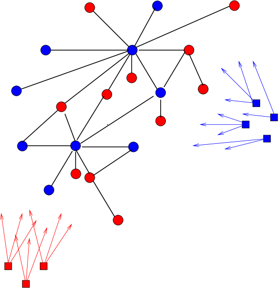
Figure 1: (color online) Representation of the voter model on a network. The different colors indicate the internal states of the voters, which can be undecided (circles), and opinion makers (squares). Opinion makers can affect all voters of the network but undecided voters can only influence their connected neighbors.

Let

$$x=\{x_{1},x_{2},\dots,x_{k-1},x_{k},x_{k+1},\dots,x_{N}\}$$ (1)

denote a microscopic state of the network with $x_{i}=0$ or $x_{i}=1$ representing the state of node $i$. There is a total of $2^{N}$ possible microscopic states and we call $P_{t}(x)$ the probability of finding the network in the state $x$ at time $t$. Since a single free node can change state per time step, it is useful to define the auxiliary state $x^{k}$ which is identical to $x$ at every node except at node $k$, whose state is the opposite of $x_{k}$, i.e., $x^{k}_{k}=1-x_{k}$. Explicitly,

$$x^{k}=\{x_{1},x_{2},\dots,x_{k-1},1-x_{k},x_{k+1},\dots,x_{N}\}.$$ (2)

With these definitions, the evolution equation for the probabilities can be written as

$$\begin{array}[]{ll}P_{t+1}(x)=pP_{t}(x)&+(1-p)\frac{1}{N}P_{t}(x)\sum_{i=1}^{N}T(x_{i}\rightarrow x_{i})\\ &+(1-p)\sum_{i=1}^{N}\frac{1}{N}P_{t}(x^{i})T(x^{i}_{i}\rightarrow x_{i}).\end{array}$$ (3)

The first two terms take into account the probability that the network is already in state $x$ and the selected node (i) does not change its state or (ii) copies the state of a neighbor which is identical to its own state. The last term is the probability that the network is in a state differing from $x$ by a single node, which is selected and copies the state of neighbor opposite to its own.

According to the dynamical rules, the transition probabilities can be written as

$$T(x_{i}\rightarrow x_{i})=\frac{1}{k_{i}+N_{0}+N_{1}}\left[\sum_{j=1}^{N}A_{ij}|1-x_{i}-x_{j}|+x_{i}N_{1}+(1-x_{i})N_{0}\right]$$ (4)

and

$$T(x^{i}_{i}\rightarrow x_{i})=\frac{1}{k_{i}+N_{0}+N_{1}}\left[\sum_{j=1}^{N}A_{ij}|x^{i}_{i}-x_{j}|+(1-x^{i}_{i})N_{1}+x^{i}_{i}N_{0}\right]$$ (5)

where $k_{i}$ is the degree of the node $i$. Using the fact that $x^{i}_{i}=1-x_{i}$ we find that the two transition probabilities are identical and obtain

$$\begin{array}[]{ll}P_{t+1}(x)&=pP_{t}(x)+\\ &\displaystyle{\frac{(1-p)}{N}\sum_{i=1}^{N}\frac{[P_{t}(x)+P_{t}(x^{i})]}{k_{i}+N_{0}+N_{1}}\left[\sum_{j=1}^{N}A_{ij}|1-x_{i}-x_{j}|+x_{i}N_{1}+(1-x_{i})N_{0}\right]}.\end{array}$$ (6)

IV Fully connected networks

For networks that are fully connected the nodes are indistinguishable and the state of the network is fully specified by the number $m$ of nodes with internal state 1 aguiar05 ; chinellato2015 . Each of these macroscopic states corresponds to a set of $N!/[(N-m)!m!]$ degenerated microscopic network states. Because there are only $N+1$ macroscopic states equations (6) are greatly simplified. The equilibrium probability $\rho_{FC}(m)$ of finding the network with $m$ nodes in state 1 is given by the Beta-Binomial distribution chinellato2015

$$\rho_{FC}(m)=A(N,N_{0},N_{1})~{}\frac{\Gamma(N_{1}+m)~{}\Gamma(N+N_{0}-m)}{\Gamma(N-m+1)~{}\Gamma(m+1)},$$ (7)

where

$$A(N,N_{0},N_{1})=\frac{\Gamma(N+1)~{}\Gamma(N_{0}+N_{1})}{\Gamma(N+N_{0}+N_{1})~{}\Gamma(N_{1})~{}\Gamma(N_{0})}.$$ (8)

This expression can also be written in term of $x_{m}=m/N$. In the limit $N\rightarrow\infty$, $x_{m}$ becomes a continuous variable $0\leq x\leq 1$ and $\rho_{FC}$ converges to the Beta distribution kirman

$$\rho_{FC}(x)=\frac{\Gamma(N_{0}+N_{1})}{\Gamma(N_{0})\Gamma(N_{1})}x^{N_{0}-1}(1-x)^{N_{1}-1}.$$ (9)

The interesting feature of the solution expressed by Eq.(7) is that for $N_{0}=N_{1}=1$ it gives $\rho_{FC}(m)=1/(N+1)$, meaning that all states are equally likely, as illustrated in Fig.2.

For networks of different topologies the effect of the fixed nodes is amplified. The probability that a free node copies a fixed node is $P_{i}=(N_{0}+N_{1})/(N_{0}+N_{1}+k_{i})$, where $k_{i}$ is the degree of the node. For fully connected networks $k_{i}=N-1$ and $P_{FC}\equiv(N_{0}+N_{1})/(N_{0}+N_{1}+N-1)$. For general networks an average value $P_{av}$ can be calculated by replacing $k_{i}$ by the average degree. Effective numbers of fixed nodes $N_{0ef}$ and $N_{1ef}$ can be then defined as the values of $N_{0}$ and $N_{1}$ in $P_{FC}$ for which $P_{av}\equiv P_{FC}$. This leads to

$$N_{0ef}=fN_{0},\qquad\qquad N_{1ef}=fN_{1},$$ (10)

where $f=(N-1)/k_{av}$. In chinellato2015 it was shown that Eq.(7) with the above rescaling of fixed nodes fits very well the probability distribution for a variety of topologies. The formula was tested for relatively small networks of the types random, 2-D regular lattice, Barabasi-Albert scale-free and small world. Similar results were obtained in the context of herding behavior of economic agents alfarano ; marketcrises11 .

V Star networks

V.1 Master equation

For a star network it is convenient to set the total number of nodes to $N+1$. Node 1 is the central node and it is connected to all peripheral $N$ nodes. The peripheral nodes, on the other hand, are only connected to the central node. The peripheral nodes are indistinguishable from each other and, similar to the fully connected network, there are only $2(N+1)$ macroscopic states, characterized by having $m$ peripheral nodes in state 1 ($N+1$ possibilities) and the central node in state 1 or 0.

The evolution equation for the macroscopic states can be obtained from equations (6) if we define $r_{1}(m,t)$ and $r_{0}(m,t)$ as the probabilities of having $m$ peripheral nodes in state 1 at time $t$ with the central node in state 1 and 0 respectively. We obtain

$$\begin{split}r_{1}(m,t+1)&=r_{1}(m,t)\left\{p+\frac{(1-p)}{(N+1)}\left[\frac{m(N_{1}+1)+(N-m)N_{0}}{(1+N_{1}+N_{0})}+\frac{(m+N_{1})}{(N+N_{0}+N_{1})}\right]\right\}\\ &+r_{1}(m+1,t)\,(1-p)\frac{(m+1)N_{0}}{(N+1)(1+N_{0}+N_{1})}\\ &+r_{1}(m-1,t)\,(1-p)\frac{(N-m+1)(N_{1}+1)}{(N+1)(1+N_{0}+N_{1})}\\ &+r_{0}(m,t)\,(1-p)\frac{(m+N_{1})}{(N+1)(N+N_{0}+N_{1})},\end{split}$$ (11)

and

$$\begin{split}r_{0}(m,t+1)&=r_{0}(m,t)\left\{p+\frac{(1-p)}{(N+1)}\left[\frac{mN_{1}+(N-m)(N_{0}+1)}{(1+N_{1}+N_{0})}+\frac{(N-m+N_{0})}{(N+N_{0}+N_{1})}\right]\right\}\\ &+r_{0}(m+1,t)\,(1-p)\frac{(m+1)(N_{0}+1)}{(N+1)(1+N_{0}+N_{1})}\\ &+r_{0}(m-1,t)\,(1-p)\frac{(N-m+1)N_{1}}{(N+1)(1+N_{0}+N_{1})}\\ &+r_{1}(m,t)\,(1-p)\frac{(N-m+N_{0})}{(N+1)(N+N_{0}+N_{1})}.\end{split}$$ (12)

The first two terms in these equations take into account the probability that the network is in the state $x$ at time $t$, and to select a node that (i) does not change its state or (ii) copies the state of a neighbor in its own state. The last three terms represent the probability that the network is in a state differing from $x$ by a single node at time $t$, to select this node, and to copy the state of a neighbor in the opposite state.

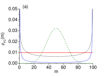
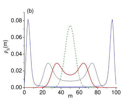
Figure 2: (color online) Equilibrium probability distribution for networks with $N=100$ nodes and different values of $N_{p}=N_{0}=N_{1}$: $N_{p}=10$ (green dashed), $N_{p}=1$ (thick red), $N_{p}=0.5$ (black dotted), $N_{p}=0.05$ (blue). (a) fully connected network; (b) star network.

The probability of having $m$ nodes in state 1 in the star network is, therefore,

$$\rho_{S}(m,t)=r_{1}(m-1,t)+r_{0}(m,t).$$ (13)

The results provided by equations (11) and (12) agree perfectly well with numerical simulations. A comparison with the fully connected network is shown in Fig.2. The main feature of these results is the different way in which the transition between ordered and disordered states occurs: instead of the meltdown of the Gaussian distribution observed for fully connected networks, the Gaussian state splits in two peaks that move toward the boundaries $m=0$ and $m=N$ as $N_{0}$ and $N_{1}$ are decreased.

V.2 Approximate solutions

The main difficulty in solving equations (11) and (12) is that they are coupled through the central node. Although we have not found exact solutions, a simple enough approximation can be readily obtained if the central node is momentarily considered to be fixed. If the central node is fixed in state 1, any peripheral node sees $N_{0}$ fixed nodes in state 0 and $N_{1}+1$ nodes fixed in state 1. The problem reduces to that of $N$ independent nodes. The asymptotic probability that a peripheral node is in state 1 is

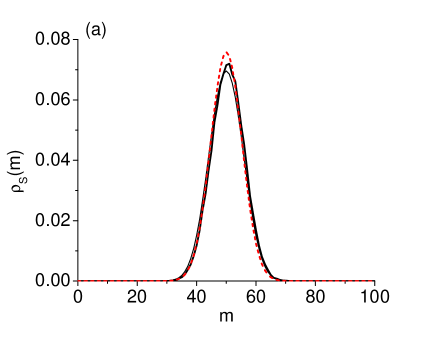
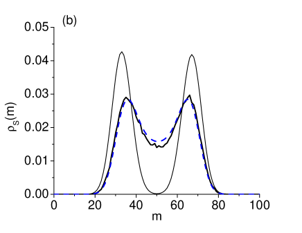
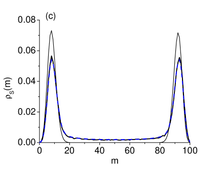
Figure 3: (color online) Comparison between numerical simulations (thick lines) and the approximate equilibrium distribution Eq.(18) (thin lines). Panel (a), for $N_{p}=10$ also shows the result for a fully connected network with the rescaling Eq.(10) corresponding to $f=99/2$ (red dashed curve). The dashed blue lines in panels (b) ($N_{p}=1$) and (c) ($N_{p}=0.1$) correspond to the approximation described in appendix A. The parameters are $T=2\times 10^{4}$, $p=0.5$, $N=100$. For the simulations $10^{5}$ realizations were performed. Panel (d) shows the distribution for different network sizes (from left to right $N=100$, $250$, $500$, $750$ and $1000$) for $N_{p}=\sqrt{N}/4$, where the peak splits in two.

$$\nu_{1}=\frac{1+N_{1}}{1+N_{0}+N_{1}}.$$ (14)

Therefore, the probability that $m$ nodes are in state 1 (the central node plus $m-1$ peripheral nodes) becomes

$$p_{1}(m)=\binom{N}{m-1}\nu_{1}^{m-1}(1-\nu_{1})^{N-m+1}.$$ (15)

Similarly, fixing the central node in the state 0, the asymptotic probability that a peripheral node is in state 1 is

$$\nu_{0}=\frac{N_{1}}{1+N_{0}+N_{1}},$$ (16)

and the probability that $m$ nodes are in state 1 is

$$p_{0}(m)=\binom{N}{m}\nu_{0}^{m}(1-\nu_{0})^{N-m}.$$ (17)

Adding these results we obtain the approximate expression

$$\rho_{S}(m)\approx\frac{N_{1}}{N_{0}+N_{1}}p_{1}(m)+\frac{N_{0}}{N_{0}+N_{1}}p_{0}(m),$$ (18)

where we have introduced the weights $N_{1}/(N_{0}+N_{1})$ and $N_{0}/(N_{0}+N_{1})$ of the central node to be in the state 1 or 0, respectively.

In this paper we will restrict our simulations to symmetric perturbations and define, for simplicity,

$$N_{p}\equiv N_{0}=N_{1}.$$ (19)

Fig.3 shows a comparison between simulations and the approximate formula (18). The two peaks are clearly related to the two states of the central node and are reasonably well described by the approximation. The region between the peaks is not well represented, since it has important contributions from flips of the central node that have been discarded. The dashed blue line shows the result of a better, although ad hoc, approximation described in the appendix that fits the entire curve with very good precision. Fig.3(a) also shows the approximation (10) obtained via rescaling of the expression for fully connected networks, which works well for $N_{p}>>1$.

The approximate solutions can also be used to estimate the point where the Gaussian-like distribution breaks in two peaks. For large $N$ the contributions $p_{0}$ and $p_{1}$ for $\rho_{S}$ become Gaussians centered at $N\nu_{0}$ and $N\nu_{1}$ with variance $\sigma^{2}=NN_{p}(1+N_{p})/(1+2N_{p})^{2}$. The two-peak structure appears when the distance between the two centers is of the order of the standard deviation. This gives $N_{p}\sim\sqrt{N}$ and numerical calculations indicate that $N_{c}\approx\sqrt{N}/4$. Fig.3(d) shows the equilibrium distribution for several values of $N$ and $N_{p}=\sqrt{N}/4$. The transition from unimodal to bimodal distribution marks the regime where the influence of the central node competes with the external perturbation, modifying the equilibrium distribution substantially with respect to the fully connected dynamics. The two peaks move apart slowly as the external perturbation is decreased and are clearly separated only when $N_{p}\sim 1$, independently of the network size $N$.

Although the equilibrium distribution of states of the star network changes smoothly as the perturbation is decreased, the transition in behavior is rather different from what is observed in the fully connected network: for $N_{p}>>\sqrt{N}$ the state is disordered, with approximately half the nodes in state 1 and half the nodes in state 0. The standard deviation is $\sigma=\sqrt{N}/2$ so that $\sigma/N=1/2\sqrt{N}$. For $N_{p}=\sqrt{N}/4$, when the two peak structure appears, the standard deviation increases by a factor of 4 to $\sigma/N=2/\sqrt{N}$. As $N_{p}$ decreases below 1 and the two peaks get significantly apart, the network is most likely to be found with either a fraction $\nu_{1}=(1+N_{p})/(1+2N_{p})$ or $\nu_{0}=N_{p}/(1+2N_{p})$ in state 1, executing fast collective transitions between the two states (see next subsection). This is in contrast with the behavior exhibited by the fully connected network, which have either most nodes 1 or most nodes 0 staying in each of these states for long periods of time before moving to the other.

V.3 Dynamics and Magnetization

In analogy with the Ising model we define the average magnetization per node as

$$M=\frac{2n_{1}}{N}-1$$ (20)

where $n_{1}$ is the number of nodes in state 1, so that $-1\leq M\leq+1$. In order to study the dynamics of $M$ we run a single simulation for each network and plot $M$ as a function of the time.

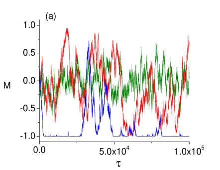
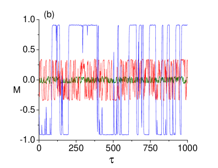
Figure 4: (color online) Magnetization for a single simulation for $N_{p}=10$ (green), $N_{p}=1$ (red) and $N_{p}=0.05$ (blue). (a) fully connected network with $N=2\times 10^{4}$ nodes; (b) star network with $N=2\times 10^{4}$ peripheral nodes. Time is measured in units of network size.

Fig. 4 shows the results for $N_{p}=10$, $1$ and $0.05$ (see also Fig. 2). In these plots one unit of time $\tau$ is a Monte Carlo step, corresponding to $N$ steps $t$ of the dynamics, so that all nodes are updated, on average, at each unit of $\tau$. For the fully connected network with $N=20000$, Fig.4(a), $M$ fluctuates around zero for $N_{p}=10$ (green line). The fluctuations increase as the critical value is approached and for $N_{p}=1$ (red line) they take the entire range of $M$. For $N_{p}=0.05$ (blue line) the system stays a substantial amount of time magnetized at $M=+1$ or $M=-1$, alternating from one extreme to the other. The lower the values of $N_{p}$ the longer the times the system stays in each state for a fixed value of $N$, and similarly for increasing $N$ for fixed $N_{p}$.

For the star network, Fig.4(b), the results show two distinct features. First, the amplitude of the oscillations increases smoothly as $N_{p}$ decreases, reflecting the position of the two peaks of the equilibrium distribution. For $N_{p}=1$, for instance, $M$ oscillates in the interval around $\pm 0.3$. Second, the oscillations are much faster, on the scale of tens of time steps for $N_{p}=0.05$, as compared to the thousands of time steps of the fully connected network. These oscillations are clearly driven by flips of the central node, which pulls the majority of the peripheral nodes with it.

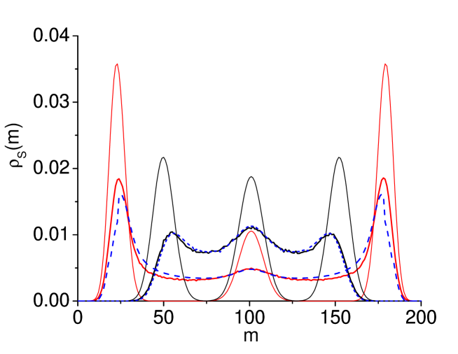
Figure 5: (color online) Equilibrium probability distribution $\rho_{S}(m)$ for a star network with $N_{c}=2$ center nodes, $N=200$ peripheral nodes and $N_{0}=N_{1}=N_{p}$ for $N_{p}=1$ (black) and $N_{p}=0.3$ (red). Thick curves show the result of simulations and thin curves the approximation given by Eq.(21). The dashed blue lines correspond to the approximation described in appendix A.

The large difference in the time scales displayed in Fig. 4 can be understood from the network topologies. For fully connected networks the time scale measured in number of time steps $t$ is well known, given by $t=N(N+2N_{p}-1)/2N_{p}$ (see chinellato2015 , for instance). For small $N_{p}$ we find $\tau\equiv t/N\simeq N/2N_{p}$. For the star network, on the other hand, the state of the peripheral nodes is controlled by the central node. If the central node is in state $0$, most of the peripheral nodes will be in state $0$ as well if $N_{p}$ is small. The probability that the central node flips from $0$ to $1$ can be estimated as the probability that it copies a frozen node in state $1$: $N_{p}/(N-1+2N_{p})\simeq N_{p}/N$. The average time for this to happen is $t=N/N_{p}$ or $\tau=t/N=1/N_{p}$. The two time scales differ by a factor $N/2$, which is consistent with the results shown by Fig. 4.

V.4 Generalizations

Star networks where the center is composed not by a single node, but by a group of totally connected nodes can also be studied within this approximation. If the center has $N_{c}$ nodes a stationary solution can be constructed by freezing the state of the center into $m$ ones and $N_{c}-m$ zeros and assigning a weight to this state according to the fully connected distribution $\rho_{FC}(m)$, given by Eq.(7). Equation (18) readily generalizes to

$$\rho(m)\approx\sum_{k=0}^{N_{c}}\rho_{FC}(k)\binom{N}{m-k}\nu_{k}^{m-k}(1-\nu_{k})^{N-m+k},$$ (21)

where

$$\nu_{k}=\frac{N_{1}+k}{N_{c}+N_{0}+N_{1}}$$ (22)

and $\rho(k)_{FC}$ is given by equation (7) with $N$ replaced by $N_{c}$. Fig. 5 shows an example with $N_{c}=2$ where a three peak structure is clearly visible close to the phase transition $N_{0}=N_{1}=1$. The approximation (21) captures well the position of the peaks, but overshoots their height to compensate for the lost interference between the peaks.

As a second application we consider the joint effect of two hubs in a complex network. If we approximate the hubs as independent star networks with a single central node, the probability of finding $m$ nodes in the state 1 is simply given by

$$\rho(m)=\sum_{j=0}^{m}\rho_{S,\,{\cal N}_{1}}(j)\rho_{S,\,{\cal N}_{2}}(m-j),$$ (23)

where we have indicated explicitly the number of nodes of each star in the distribution. For small values of $N_{p}$, the separate distributions will have two peaks, centered at, say, $m_{1}$ and ${\cal N}_{1}-m_{1}$; $m_{2}$ and ${\cal N}_{2}-m_{2}$ respectively. The joint distribution given by Eq.(23) will display four peaks at $m_{1}+m_{2}$, ${\cal N}_{1}-m_{1}+m_{2}$, ${\cal N}_{2}-m_{2}+m_{1}$ and ${\cal N}_{1}+{\cal N}_{2}-m_{1}-m_{2}$. If the hubs are not independent, but coupled by only a few links, we expect this peak structure to persist.

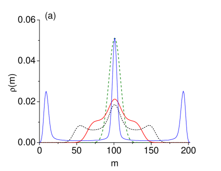
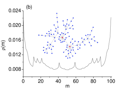
Figure 6: (color online) (a) Equilibrium distribution for a pair of independent star networks with ${\cal N}_{1}=101$ and ${\cal N}_{2}=11$ nodes for $N_{p}=10$ (green dashed), $N_{p}=1$ (thick red), $N_{p}=0.5$ (black dotted) and $N_{p}=0.05$ (blue). (b) Distribution for a scale-free network with $100$ nodes and $N_{p}=0.01$. The two largest hubs (shown in red in the inset) have 16 and 13 peripheral nodes and are connected by their centers.

Figure 6(a) shows the stationary distribution for two independent star networks of sizes ${\cal N}_{1}=101$ and ${\cal N}_{2}=11$. The splitting of the Gaussian-like peak in two occurs at $N_{0}=N_{1}\approx 2.6$ and $N_{0}=N_{1}\approx 0.8$, respectively. However, because the separation between the two peaks of the smaller star is small, its effect is felt only at much smaller values of the perturbation, when the two peaks of the large hub approach the borders and the distribution becomes thin. Fig. 6(b) shows the equilibrium distribution for a more complex network with 100 nodes constructed with preferential attachment. The network has two main hubs (shown in red in the inset) with 16 and 13 peripheral nodes, respectively. The peaks in the distribution are signatures of the hubs. For scale-free networks with more cycles (not shown) the presence of the peaks is much less conspicuous and the distribution becomes again similar to the fully connected case with rescaled perturbations.

VI Conclusions

The voter model with opinion makers is one of the simplest dynamical systems that can be represented on a network. It models an election between candidates where the voters are influenced by their social contacts and by external factors such as journalists and politicians. If the number of opinion makers is zero the population is certain to reach a consensus toward one of the candidates independently of the structure of the network. The power of the opinion makers, however, depends strongly on the average degree of the network. For a completely connected network the transition between nearly consensus (ordered state) and a tie (disordered state) takes place exactly at $N_{0}=N_{1}=1$, independently of the population size $N$. For networks with average degree $k_{av}$ the effect of the fixed nodes is amplified by a factor $f=(N-1)/k_{av}$, which can be very large for natural populations. Much above or much below the transition from disordered to ordered states the influence of the network structure is negligible and only shows up in the rescaling of the opinion makers influence, that is large when the network is weakly connected. This is in contrast with processes describing the spreading of epidemics or synchronization of oscillators, where the topology plays a crucial role barrat08 ; ves01 ; pecora02 ; motter03 ; pac04 ; laguna ; guime ; aguiar05 ; rodrigues13 ; rodrigues14 . Close to the critical point, however, the network structure can leave signatures in the probability distribution $\rho(m)$.

For the particular case of star networks with a single central node, the Gaussian-like distribution displayed by $\rho_{S}(m)$ for large values of $N_{0}$ and $N_{1}$ splits into two peaks centered at $N(N_{1}+1)/(N_{1}+N_{0}+1)$ and $NN_{1}/(N_{1}+N_{0}+1)$ reflecting the state of the central node being 1 or 0. The central node controls the entire system and the distribution behaves approximately as a single giant node with two collective states only. For $N_{0}=N_{1}=1$ the peaks are centered at $2N/3$ and $N/3$ respectively, which is rather different from the distribution of fully connected networks where $\rho_{FC}(m)=1/(N+1)$ is constant. In the former case the election will be won by one of the candidates with approximately $67\%$ of the votes, whereas in the latter, the winner can have any number of votes with equal probability. For small values of $N_{0}$ and $N_{1}$ both star and fully connected networks are likely to be found in ordered states, where most nodes are in state 0 or in state 1. These states, however, are not stable and network oscillates between the two possibilities. We found that the average frequency of these oscillations are much higher for star networks than for fully connected ones.

When a few weakly connected hubs are present, the effects of central nodes are still visible, as shown by Fig.6(b). However, when the system is controlled by multiple hubs, as in a general scale-free network, the collective behavior becomes again similar to that predicted by the mean field approximation and the control by ‘local leaders’ becomes much less relevant. In these cases Eqs.(7) and (10) provide good approximations for the equilibrium probability.

As a final remark we note that fully connected and stars with arbitrary number of central nodes seem to be the only network topologies where a simple treatment via macroscopic master equations similar to (11)-(12) is possible. Even the highly symmetric ring network (1-D lattice with periodic boundary conditions) does not behave as if all nodes were identical, since different configuration having the same number of nodes at the state 1 give rise to different macroscopic states.

M.A.M.A. and D.M.S. acknowledge financial support from CNPq and FAPESP. C.A.M. was supported by CAPES.

Appendix A An ad hoc approximation for the equilibrium distribution

The approximation (18) completely discards the fact that the state of the central node fluctuates and fails to describe the region between the two peaks. Here we derive a better approximation using phenomenological ideas. We first define

$$\nu(x)=\frac{x+N_{1}}{1+N_{0}+N_{1}}.$$ (24)

as the equivalent of (14) and (16) for the case where the state of the central node is in the average state $x$ with $0\leq x\leq 1$. Accordingly, we define

$$p(x,m)=\frac{\Gamma(N+1)}{\Gamma(N-m+x+1)\Gamma(m-x+1)}\nu(x)^{m-x}(1-\nu(x))^{N-m+x}$$ (25)

as the probability of finding $m$ nodes in state 1, including the central the peripheral nodes (see eqs. (17) and (15)). If $c(x)$ is the probability distribution that the central node is in state $x$, then

$$\rho(m)=\int_{0}^{1}dx\,c(x,N_{0},N_{1})p(x,m).$$ (26)

For

$$c(x,N_{0},N_{1})=\frac{N_{0}}{N_{0}+N_{1}}\delta(x)+\frac{N_{1}}{N_{0}+N_{1}}\delta(x-1)$$ (27)

we recover the approximation (18).

In order to obtain better results we need to consider smoother distributions and the natural functional dependence for $c(x)$ is the continuous version of $\rho_{FC}$, the Beta distribution eq.(9):

$$c(x,N_{0},N_{1})=\frac{\Gamma(n_{0}+n_{1})}{\Gamma(n_{0})\Gamma(n_{1})}x^{n_{0}-1}(1-x)^{n_{1}-1}.$$ (28)

Here $n_{0}(N_{0},N_{1})$ and $n_{1}(N_{0},N_{1})$ measure the joint effect of the external perturbations, $N_{0}$ and $N_{1}$, and of the $N-1$ peripheral nodes on the central node. Because the approximation with the delta functions (27) already gives a good description of the exact distribution, $n_{0}$ and $n_{1}$ should be significant only close to the phase transition. The choice

$$n_{0}(N_{0},N_{1})=N_{0}e^{-(N_{0}+N_{1})/2}\qquad n_{1}(N_{0},N_{1})=N_{1}e^{-(N_{0}+N_{1})/2}$$ (29)

turns out to work well for all the cases tested.

For the case of two central nodes (see Fig.5) a similar procedure can be divised. We set

$$\nu(x,y)=\frac{x+y+N_{1}}{2+N_{0}+N_{1}}$$ (30)

with $x$ and $y$ representing the states of the two central nodes. The probability that $m$ nodes are in state 1 becomes

$$p(x,y,m)=\frac{\Gamma(N+1)}{\Gamma(N-m+x+y+1)\Gamma(m-x-y+1)}\nu(x,y)^{m-x-y}(1-\nu(x,y))^{N-m+x+y}$$ (31)

so that

$$\rho(m)=\int_{0}^{1}dx\,\int_{0}^{1}dy\,c(x,y,N_{0},N_{1})p(x,y,m).$$ (32)

The probability distribution that the two central nodes are in states $x$ and $y$ must reproduce the coefficients $\rho_{FC}(k)$ in Eq.(21). Using the analogy between Eqs. (18) and (27) it can be checked that the appropriate function is

$$c_{2}(x,y,N_{0},N_{1})=c(x,N_{0},N_{1})\,c(y,N_{0}+1-x,N_{1}+x).$$ (33)

Indeed, using the approximation (27) for $c(x,N_{0},N_{1})$ we see that

$$\begin{array}[]{ll}c_{2}(x,y,n_{0},n_{1})&\approx\frac{1}{(N_{0}+N_{1})(1+N_{0}+N_{1})}\times\left\{N_{0}(N_{0}+1)\delta(x)\delta(y)\right.\\ \\ &\left.+N_{0}N_{1}[\delta(x)\delta(1-y)+\delta(1-x)\delta(y)]+N_{1}(N_{1}+1)\delta(1-x)\delta(1-y)\right\}\end{array}$$ (34)

whose coefficients correspond to $\rho_{FC}(k)$. We remark that the integrals (26) and (32) might be difficult to evaluate numerically for very small values of $N_{0}$ and $N_{1}$, since the Beta distribution becomes very large close to $x=0$ and $x=1$. In this limit, however, the distribution is peaked close to $m=0$ and $m=N$ and the approximation provided by the fully connected distribution should work well.

References

- (1) R. Albert and A.-L. Barabasi, Rev. Mod. Phys. 74, 47 (2002).
- (2) S. Boccaletti, V. Latora, Y. Moreno, M. Chavez and D.-U. Hwang, Phys. Rep. 424, 175 (2006).
- (3) M.E.J. Newman, SIAM Review 45, 167 (2003).
- (4) M.E. J. Newman, Networks: An Introduction, Oxford University Press, 2010.
- (5) O. Sporns, Networks of the Brain The MIT Press, Cambridge, 2011.
- (6) Adaptive Networks. Theory, Models and Applications (Understanding Complex Systems). T. Gross and H. Sayama, (eds.) (Springer-Verlag: Berlin, 2009)
- (7) Y. Bar-Yam and I. Epstein, PNAS 101, 4341 (2004).
- (8) R. Albert, H. Jeong, and A.-L. Barabasi, Nature 406, 378 (2000).
- (9) Buldyrev, S. V., Parshani, R., Paul, G., Stanley, H. E., and Havlin, S. Nature 464, 1025-1028 (2010).
- (10) R. Cohen, K. Erez, D. ben-Avraham, and S. Havlin, Phys. Rev. Lett. 85, 4626 (2000).
- (11) A. Barrat, M. Barthelemy, and A. Vespignani (2008). Dynamical processes on complex networks (Vol. 1). Cambridge: Cambridge University Press.
- (12) R. Pastor-Satorras and A. Vespignani, Phys. Rev. Lett. 86, 3200 (2001).
- (13) M. Barahona and L.M. Pecora, Phys. Rev. Lett. 89, 054101 (2002).
- (14) T. Nishikawa, A.E. Motter, Y.-C. Lai, and F.C. Hoppensteadt, Phys. Rev. Lett. 91, 014101 (2003).
- (15) Y. Moreno, M. Nekovee and A.F. Pacheco, Phys. Rev. E 69, 066130 (2004).
- (16) M.F. Laguna, A. Guillermo, and D. H. Zanette, Physica A 329, 459 (2003).
- (17) R. Guimera, A. Diaz-Guilera, F. Vega-Redondo, A. Cabrales, and A. Arenas, Phys. Rev. Lett. 89, 248701 (2002).
- (18) M.A.M. de Aguiar, I.R. Epstein and Y. Bar-Yam, Phys. Rev. E 72, 067102 (2005).
- (19) Peng Ji, T. K. DM. Peron, P. J. Menck, F. A. Rodrigues, and J. Kurths, Phys. Rev. Lett. 110, 218701 (2013)
- (20) G. F. de Arruda, A. L. Barbieri, P. M. Rodriguez, F. A. Rodrigues, Y. Moreno, and L.F. Costa, Phys. Rev. E 90, 032812 (2014)
- (21) S.A. Hill and D. Braha, Phys. Rev. E 82(4), 046105 (2010).
- (22) X. Wang, Y.-C. Lai, and C. H. Lai, Phys. Rev. E 74, 066104 (2006).
- (23) E.J. Lee, K.-I. Goh, B. Kahng, and D. Kim, Phys. Rev. E 71, 056108 (2005).
- (24) D. Harmon, M. Lagi, M.A.M. de Aguiar, D.D. Chinellato, D. Braha, I.R. Epstein and Y. Bar-Yam, PLoS ONE 10(7) e0131871 (2015). doi:10.1371/journal.pone.0131871
- (25) D. D. Chinellato, M. A. M. de Aguiar, I. R. Epstein, D. Braha, and Y. Bar-Yam, J. Stat. Phys. 159, 221 (2015).
- (26) Rick Quax, Andrea Apolloni, Peter M. A. Sloot, J. R. Soc. Interface 10: 20130568 (2013)
- (27) R. Cohen, K. Erez, D. ben-Avraham, S. Havlin, Phys. Rev. Lett. 86 (2001) 3682.
- (28) D.S. Callaway, M.E.J. Newman, S.H. Strogatz, D.J. Watts Phys. Rev. Lett. 85, 5468 (2000).
- (29) Martijn P. van den Heuvel and Olaf Sporns. Trends in Cognitive Sciences, 17 683-96 (2013).
- (30) T. M. Liggett, Interacting Particles Systems (Springer, New York, 1985).
- (31) E. Yildiz, A. Ozdaglar, D. Acemoglu, A. Saberi and A. Scaglione, ACM Trans. Econ. Comp. 1, 4, Article 19 (2013). DOI:http://dx.doi.org/10.1145/2538508
- (32) D. Vilone and C. Castellano, Phys. Rev. E 69, 016109 (2004).
- (33) V. Sood and S. Redner, Phys. Rev. Lett. 94, 178701 (2005).
- (34) P.A.P. Moran, Proc. Cambridge Philos. Soc. 54, 60 (1958).
- (35) M.A.M. de Aguiar and Y. Bar-Yam, Phys. Rev. E 84, 031901 (2011).
- (36) A. Kirman, Quarterly Journal of Economics, 108 137 (1993).
- (37) R.J. Glauber, J. Math. Phys. 4, 294 (1963)
- (38) V. Sood and S. Redner, Phys. Rev. E 77, 041121 (2008).
- (39) F. Vazquez and V. Eguiluz, New J. Phys. 10, 063011 (2008).
- (40) M. Mobilia, Phys. Rev. Lett. 91, 028701 (2003).
- (41) M. Mobilia, A. Petersen, S. Redner, J. Stat. Mech. P08029 (2007) doi:10.1088/1742-5468/2007/08/P08029.
- (42) S. Alfarano, M. Milakovic, J. of Economic Dynamics and Control 33 78 (2009).