Vestigial chiral and charge orders from bidirectional spin-density waves: Application to the iron-based superconductors

Abstract

Recent experiments in optimally hole-doped iron arsenides have revealed a novel magnetically ordered ground state that preserves tetragonal symmetry, consistent with either a charge-spin density wave (CSDW), which displays a non-uniform magnetization, or a spin-vortex crystal (SVC), which displays a non-collinear magnetization. Here we show that, similarly to the partial melting of the usual stripe antiferromagnet into a nematic phase, either of these phases can also melt in two stages. As a result, intermediate paramagnetic phases with vestigial order appears: a checkerboard charge density-wave for the CSDW ground state, characterized by an Ising-like order parameter, and a remarkable spin-vorticity density-wave for the SVC ground state – a triplet d-density wave characterized by a vector chiral order parameter. We propose experimentally detectable signatures of these phases, show that their fluctuations can enhance the superconducting transition temperature, and discuss their relevance to other correlated materials.

I Introduction

One of the hallmarks of the superconducting state of the iron-based materials reviews is its typical proximity to a stripe magnetically ordered state, with spins aligned parallel to each other along one in-plane direction and anti-parallel along the other (see Fig. 1a) Dagotto12 . As a result, this stripe state breaks two distinct symmetries of the high-temperature paramagnetic-tetragonal state: a continuous spin-rotational $O(3)$ symmetry and an Ising-like $Z_{2}$ symmetry related to the equivalence of the $x$ and $y$ directions Fang08 ; Xu08 ; Johannes09 ; Eremin10 ; Abrahams11 ; Fernandes12 ; Dagotto14 . Magnetic fluctuations present in the paramagnetic state can cause these two symmetries to be broken at different temperatures, giving rise to an intermediate nematic phase that preserves the spin-rotational $O(3)$ symmetry but, as a “vestige” of the stripe order Kivelson14 , breaks the tetragonal $Z_{2}$ symmetry Fernandes14 . Indeed, in the phase diagrams of most iron-based superconductors, the magnetic transition line is closely followed by the structural/nematic one at slightly higher temperatures. The corresponding nematic degrees of freedom impact not only the normal state electronic properties Fisher10 ; Davis10 ; ZXshen11 ; Fisher12 ; Matsuda12 ; Gallais13 ; Dai14 ; Rosenthal14 ; w_ku10 ; Devereaux12 but also the onset and gap structure of the superconducting state Fernandes_Millis ; Lederer14 ; Kang14 .

Recently, experiments in the hole-doped pnictides $\text{Ba}(\text{Fe}_{1-x}\text{Mn}_{x})_{2}\text{As}_{2}$ Kim10 , $(\text{Ba}_{1-x}\text{Na}_{x})\text{Fe}_{2}\text{As}_{2}$ Avci14 , and $(\text{Ba}_{1-x}\text{K}_{x})\text{Fe}_{2}\text{As}_{2}$ Bohmer14 have revealed another type of magnetically ordered state that does not break the tetragonal $Z_{2}$ symmetry of the lattice. Neutron scattering experiments Kim10 ; Avci14 showed that its magnetic Bragg peaks are at the same momenta as in the stripe magnetic phase – namely, $\mathbf{Q}_{1}=\left(\pi,0\right)$ and $\mathbf{Q}_{2}=\left(0,\pi\right)$ in the Fe-only Brillouin zone. Consequently, it has been proposed Avci14 ; xiaoyu14 ; Wang_arxiv_14 ; Kang15 ; Gastiasoro15 that the tetragonal magnetic state is the realization of one of two possible biaxial (i.e. double-$\mathbf{Q}$) magnetic orders Eremin10 ; Lorenzana08 ; giovannetti ; Brydon11 . One possibility is a “charge-spin density wave” (CSDW), displaying a non-uniform magnetization which vanishes at the even lattice sites and is staggered along the odd lattice sites (Fig. 1b). The other option is a “spin-vortex crystal” (SVC), in which the magnetization is non-collinear (but coplanar) and forms spin vortices staggered across the plaquettes (Fig. 1c). Both CSDW and SVC phases are tetragonal, but have a unit cell four times larger than the paramagnetic phase. Interestingly, in $(\text{Ba}_{1-x}\text{Na}_{x})\text{Fe}_{2}\text{As}_{2}$ and $(\text{Ba}_{1-x}\text{K}_{x})\text{Fe}_{2}\text{As}_{2}$, the tetragonal magnetic state is observed very close to optimal doping Avci14 ; Bohmer14 , where superconductivity displays its highest transition temperature. Therefore, understanding the properties of these biaxial tetragonal magnetic phases is important to assess their relevance for the superconductivity.

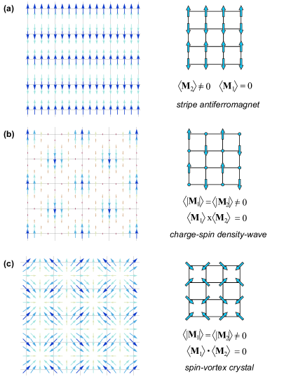
Figure 1: Magnetic ground states of the iron pnictides: (a) stripe antiferromagnet, (b) charge-spin density-wave (CSDW), (c) spin-vortex crystal (SVC). The first is orthorhombic with a doubled unit cell; the latter two remain tetragonal but with a quadrupled unit cell. $\mathbf{M}_{1}$ and $\mathbf{M}_{2}$ are the magnetic order parameters corresponding to the ordering vectors $\mathbf{Q}_{1}=\left(\pi,0\right)$ and $\mathbf{Q}_{2}=\left(0,\pi\right)$. The left panels are the actual spin density-wave patterns in real space, whereas the right panels are schematic representations focusing on the magnetization at the lattice sites.

In this paper, we show that both the CSDW and the SVC magnetic phases support composite order parameters that can condense at temperatures above the onset of magnetic order, and whose fluctuations can help enhancing $T_{c}$. As with the nematic phase, these partially ordered phases are paramagnetic, i.e. fluctuations restore the time-reversal symmetry that is broken in the ground state. In contrast to the nematic phase, however, they preserve the point group symmetry of the lattice, but break other symmetries, including translational symmetry Chern12 . In particular, upon melting the CSDW phase, we find a vestigial Ising-like charge-density wave (CDW) phase with ordering vector $\mathbf{Q}_{1}+\mathbf{Q}_{2}=\left(\pi,\pi\right)$, in which the previously magnetized sites acquire a different charge than the previously non-magnetized sites. On the other hand, upon melting the SVC ground state, we find a vestigial phase that retains memory of the preferred plane of magnetization (in spin space), and of the staggering of the spin vortices across the plaquettes. This spin-vorticity density-wave (SVDW) is a triplet d-density wave characterized by a vector chiral order parameter, which is manifested as a spin-current density-wave with modulation $\mathbf{Q}_{1}+\mathbf{Q}_{2}=\left(\pi,\pi\right)$. Besides shedding light on the magnetism of hole-doped iron pnictides, our results provide a novel microscopic mechanism for the formation of d-density waves, which have also been proposed in cuprates Chakravarty01 and heavy fermions Chakravarty14 .

The paper is organized as follows: in Section II we present the theoretical model that gives rise to the vestigial CDW and SVDW orders. Section III discusses the implications of these vestigial orders for both the normal state and superconducting state properties. Concluding remarks are presented in Section IV. To make the paper transparent and accessible, all formal details are presented in appendices. Appendix A contains the derivation of the saddle-point equations that give the phase diagram of the SVDW phase discussed in Section II. In Appendix B we derive microscopically the free energy discussed in Section III. Finally, Appendix C presents the derivation of the effective pairing interactions promoted by CDW and SVDW fluctuations discussed in Section III.

II Theoretical model for the vestigial phases

II.1 Effective action

We define two magnetic order parameters, $\mathbf{M}_{1}$ and $\mathbf{M}_{2}$, associated with the two ordering vectors $\mathbf{Q}_{1}=\left(\pi,0\right)$ and $\mathbf{Q}_{2}=\left(0,\pi\right)$, respectively. Thus, the local spin is given by $\mathbf{S}\left(\mathbf{r}\right)=\sum_{i}\mathbf{M}_{i}\mathrm{e}^{i\mathbf{Q}_{i}\cdot\mathbf{r}}$. As discussed in Refs. Eremin10 ; Fernandes12 ; xiaoyu14 ; Wang_arxiv_14 ; Kang15 ; Lorenzana08 ; giovannetti ; Brydon11 , the most general lowest order action that respects the tetragonal and spin-rotational symmetries is given by:

$$\mathcal{S}\left[\mathbf{M}_{i}\right] =\int_{q}\chi_{q}^{-1}\left(\mathbf{M}_{1}^{2}+\mathbf{M}_{2}^{2}\right)+\frac{u}{2}\int_{x}\left(\mathbf{M}_{1}^{2}+\mathbf{M}_{2}^{2}\right)^{2}$$

$$-\frac{g}{2}\int_{x}\left(\mathbf{M}_{1}^{2}-\mathbf{M}_{2}^{2}\right)^{2}+2w\int_{x}\left(\mathbf{M}_{1}\cdot\mathbf{M}_{2}\right)^{2}\ .$$ (1)

For simplicity, we will consider the finite temperature problem, but the same conclusions can be extended to the quantum case. Here, $\int_{q}\equiv\int\frac{d^{d}q}{\left(2\pi\right)^{d}}$ and $\int_{x}\equiv\int d^{d}x$ where $\mathbf{q}$ is the momentum and $\mathbf{x}$ is the position. In the neighborhood of a finite $T$ magnetic transition, and for a quasi-2D system, we can use the small $q$ expansion $\chi_{q}^{-1}\approx r_{0}+q_{\parallel}^{2}+J_{z}\sin^{2}\frac{q_{z}}{2}$, where $r_{0}$ is the distance to the mean-field magnetic critical point.

The quartic coefficients $u$, $g$, $w$ determine the nature of the magnetic ground state. These are, in turn, sensitive to microscopic considerations. The localized $J_{1}$-$J_{2}$ model favors positive $g$ and $w$ chandra . On the other hand, itinerant approaches (at weak and strong coupling) have found parameter regimes in which $g$ and $w$ can be either positive or negative Eremin10 ; Fernandes12 ; xiaoyu14 ; Wang_arxiv_14 ; Kang15 ; Lorenzana08 ; giovannetti ; Brydon11 ; Berg10 . For $g>\max\left(0,-w\right)$, the energy is minimized by the stripe state shown in Fig. 1a, in which either $\left\langle\mathbf{M}_{1}\right\rangle=0$ or $\left\langle\mathbf{M}_{2}\right\rangle=0$. Thus, in addition to breaking the $O(3)$ spin-rotational symmetry, the magnetic ground state spontaneously breaks a $Z_{2}$ symmetry by selecting one of the two order parameters to be non-zero. Since $\mathbf{M}_{1}$ and $\mathbf{M}_{2}$ are related by a $90^{\circ}$ rotation, once this $Z_{2}$ symmetry is broken the tetragonal symmetry of the system is lowered to orthorhombic (see Fig. 2a). A composite Ising-nematic order parameter, living on the bonds of the lattice, can be identified by performing a Hubbard-Stratonovich transformation on the quartic term with coefficient $g$, yielding $\left\langle\varphi_{\mathrm{nem}}\right\rangle=g\left\langle\mathbf{M}_{1}^{2}-\mathbf{M}_{2}^{2}\right\rangle$. Because $Z_{2}$ is a discrete symmetry, while spin-rotational $O(3)$ is a continuous symmetry, a strongly anisotropic 3D system will generically display a vestigial paramagnetic nematic phase where $\left\langle\mathbf{M}_{i}\right\rangle=0$ but $\left\langle\varphi_{\mathrm{nem}}\right\rangle\neq 0$ Fang08 ; Fernandes12 ; Batista11 .

For $g<\max\left(0,-w\right)$, the ground state of Eq. (1) is no longer a uniaxial magnetic stripe state, but a biaxial magnetic state with $|\left\langle\mathbf{M}_{1}\right\rangle|=|\left\langle\mathbf{M}_{2}\right\rangle|$ that preserve tetragonal symmetry. If $w<0$, the energy is minimized by $\left\langle\mathbf{M}_{1}\right\rangle\parallel\left\langle\mathbf{M}_{2}\right\rangle$, which in terms of the local spin configuration $\mathbf{S}\left(\mathbf{r}\right)$ corresponds to a non-uniform state as depicted in Fig. 1b. We identify this state as a charge-spin density-wave (CSDW). On the other hand, if $w>0$, the energy minimization gives $\left\langle\mathbf{M}_{1}\right\rangle\perp\left\langle\mathbf{M}_{2}\right\rangle$, corresponding to a non-collinear, coplanar spin configuration (see Fig. 1c). This state is identified as a spin vortex-crystal (SVC). We now discuss whether these tetragonal magnetic phases can melt in a two-stage process, giving rise to vestigial orders akin to the nematic phase.

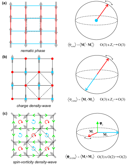
Figure 2: The vestigial composite states associated with (a) the stripe antiferromaget, (b) the CSDW state, and (c) the SVC state. The real-space spins (in gray) and the magnetic order parameters in spin space (red and blue arrows, representing $\mathbf{M}_{1}$ and $\mathbf{M}_{2}$, respectively) should be understood as fluctuating, i.e. $\left\langle\mathbf{M}_{i}\right\rangle=0$ in all cases. In (a), the vestigial state is nematic (unequal blue and red bonds), associated with selecting between $\mathbf{M}_{1}$ and $\mathbf{M}_{2}$ fluctuations in spin space. The original unit cell is shown as a dashed square. In (b), the vestigial state breaks translational symmetry via a checkerboard charge density-wave (unequal blue and red sites). $\mathbf{M}_{1}$ and $\mathbf{M}_{2}$ are locked to be collinear in spin space. In (c), the vestigial spin-vorticity density-wave state breaks inversion and translational symmetries via a staggered pattern of spin vortices in the center of the plaquettes (unequal blue and red plaquettes). The corresponding spin-current pattern is shown by the green arrows. Because $\mathbf{M}_{1}$ and $\mathbf{M}_{2}$ are locked to be orthogonal in spin space, the residual spin-rotational symmetry is $O(2)$ instead of $O(3)$. Both (b) and (c) preserve tetragonal symmetry, as shown by the dashed-line unit cell.

II.2 Charge-spin density-wave

Consider the CSDW state: Once the magnetization direction is chosen by spontaneous breaking of the $O(3)$ spin-rotational symmetry, there remains a four-fold degeneracy corresponding to whether $\mathbf{M}_{1}$ and $\mathbf{M}_{2}$ are parallel or anti-parallel to the chosen direction. As is apparent in Fig. 1b, this corresponds to the breaking of translational symmetry, leading to a four-site unit cell. Notice, however, that the product of a translation by the vector $\hat{\mathbf{x}}+\hat{\mathbf{y}}$ followed by time-reversal is preserved. Thus, there is an essential $Z_{2}$ symmetry that interchanges the magnetic and non-magnetic sublattices of the CSDW state.

The order parameter field for this $Z_{2}$ symmetry is obtained via a Hubbard-Stratonovich transformation on the quartic term with coefficient $2w$ in Eq. (1), $\left\langle\varphi_{\mathrm{CDW}}\right\rangle=2\left|w\right|\left\langle\mathbf{M}_{1}\cdot\mathbf{M}_{2}\right\rangle$. Clearly, $\varphi_{\mathrm{CDW}}$ is a scalar that carries momentum $\mathbf{Q}_{1}+\mathbf{Q}_{2}=\left(\pi,\pi\right)$, i.e. the condensed phase is a CDW that doubles the unit cell, but leaves time-reversal and the tetragonal symmetry of the lattice intact (see Fig. 2b). Thus, in real space, the CDW order parameter lives on the lattice sites. The fact that the unit cell decreases from four to two sites upon going from the CSDW to the CDW phase is due to the restoration of time-reversal symmetry, which implies the restoration of the translational symmetry by $\hat{\mathbf{x}}+\hat{\mathbf{y}}$. A simple change of variables in Eq. (1), $\mathbf{M}_{1}\to 2^{-1/2}[\mathbf{M}_{1}+\mathbf{M}_{2}]$ and $\mathbf{M}_{1}\to 2^{-1/2}[\mathbf{M}_{1}-\mathbf{M}_{2}]$, interchanges the identities of the two scalar orders, $\varphi_{\mathrm{nem}}\leftrightarrow\varphi_{\mathrm{CDW}}$, but leaves the form of $\mathcal{S}$ unchanged albeit with $\left(g,w\right)\rightarrow-\left(w,g\right)$. Thus, the properties of the CDW phase are akin to those of the Ising-nematic phase – in particular, a quasi-2D system will again display for a range of intermediate temperatures a phase with $\left\langle\mathbf{M}_{i}\right\rangle=0$ but $\left\langle\varphi_{\mathrm{CDW}}\right\rangle\neq 0$.

II.3 Spin-vorticity density-wave

Consider now the SVC state, characterized by two equal magnitude orthogonal vectors $\mathbf{M}_{1}$ and $\mathbf{M}_{2}$. Upon fixing the direction of $\mathbf{M}_{1}$, which breaks the $O(3)$ spin-rotational symmetry, there remains an additional $O(2)$ symmetry related to choosing $\mathbf{M}_{2}$ in any direction along the plane perpendicular to $\mathbf{M}_{1}$ footnote-symmetries . Thus, the SVC phase can be completely characterized by a pseudo-vector order parameter $\boldsymbol{\varphi}_{\mathrm{SVDW}}$ that specifies the ordering plane which contains $\mathbf{M}_{1}$ and $\mathbf{M}_{2}$, and also by the orientation of $\mathbf{M}_{1}$ within that plane. $\boldsymbol{\varphi}_{\mathrm{SVDW}}$ is obtained via a Hubbard-Stratonovich transformation of the quartic term $w\left(\mathbf{M}_{1}\cdot\mathbf{M}_{2}\right)^{2}\to-w\left(\mathbf{M}_{1}\times\mathbf{M}_{2}\right)^{2}$ in Eq. (1), yielding $\left\langle\boldsymbol{\varphi}_{\mathrm{SVDW}}\right\rangle=2w\left\langle\mathbf{M}_{1}\times\mathbf{M}_{2}\right\rangle$, which can be identified as a vector chirality Batista09 ; footnote-inversion . Thus, upon approaching the SVC phase from high-temperatures or by melting it, there can be an intermediate state where $\left\langle\boldsymbol{\varphi}_{\mathrm{SVDW}}\right\rangle\neq 0$ but the orientation of $\mathbf{M}_{1}$ is not fixed, $\left\langle\mathbf{M}_{1}\right\rangle=0$. This chiral paramagnetic state preserves time-reversal symmetry and retains the memory of the staggering pattern of spin vortices along the plaquettes in the SVC phase, and is therefore called a spin-vorticity density-wave (SVDW) footnote-inversion . Note that the vector chiral order parameter produces an emergent Dzyaloshinskii-Moriya coupling $\boldsymbol{\varphi}_{\mathrm{SVDW}}\cdot\left(\mathbf{M}_{1}\times\mathbf{M}_{2}\right)$ relating the translational symmetry-breaking to a preferred “handedness” in spin-space. In the SVDW state, not only is the translational symmetry lowered by the doubling of the unit cell (since $\boldsymbol{\varphi}_{\mathrm{SVDW}}$ carries momentum $\mathbf{Q}_{1}+\mathbf{Q}_{2}=\left(\pi,\pi\right)$), but also the soft spin fluctuations near the magnetic transition are constrained to lie in the plane defined by $\boldsymbol{\varphi}_{\mathrm{SVDW}}$ (see Fig. 2c).

Because $\boldsymbol{\varphi}_{\mathrm{SVDW}}$ breaks a continuous $O(3)$ symmetry, there are two Goldstone modes in the SVDW phase. Consequently, in contrast to the Ising-nematic cases, the Mermin-Wagner theorem does not ensure the existence of the SVDW phase even in the two-dimensional limit. To investigate whether $\left\langle\boldsymbol{\varphi}_{\mathrm{SVDW}}\right\rangle\neq 0$ while $\left\langle\mathbf{M}_{1}\right\rangle=0$ is possible, we calculated the phase diagram for a magnetic SVC ground state treating the action in Eq. (1) in the saddle point approximation (see Appendix A). We find that for a strongly anisotropic system, i.e. $J_{z}\ll w$, there is a wide range of values of $u/w$ for which there are two transitions, with an intermediate SVDW phase and a low-temperature SVC phase (see Fig. 3). However, in this approximation, the transition to the SVDW phase is always first-order.

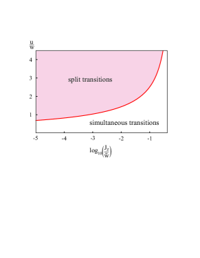
Figure 3: Phase diagram, within the saddle-point approximation, of the coupled SVDW paramagnetic and SVC magnetic transitions. In the shaded area, where the out-of-plane anisotropy is strong, the two transitions are split. The tuning parameters are the Ginzburg-Landau coefficients $u$ and $w$ (see Eq. 1) and the magnetic coupling between layers $J_{z}$. The parameter $\bar{w}$ is given by $w=T_{N,0}w/2\pi$, as discussed in Appendix B.

Spin rotational symmetry is not an exact symmetry of nature, and indeed most iron pnictides display a sizable spin anisotropy Matan09 ; Dai13 ; Tucker14 . Because the ordered moments tend to point parallel to the FeAs plane, the most significant effects of spin-orbit coupling can be captured phenomenologically in Eq. (1) by including an easy-plane anisotropy term $\kappa\left(M_{1,z}^{2}+M_{2,z}^{2}\right)$ with coupling constant $\kappa>0$ Christensen15 . The spin rotational symmetry is thus reduced to $O(2)$ and the SVDW chiral order parameter becomes the pseudo-scalar $\varphi_{\mathrm{SVDW}}=2w\left(\mathbf{M}_{1}\times\mathbf{M}_{2}\right)\cdot\hat{\mathbf{z}}$, which only breaks a discrete chiral $Z_{2}$ symmetry. For such $O(2)\times Z_{2}$ model, it is known from both numerical and analytical investigations that in $2$D the $Z_{2}$ symmetry is broken at higher temperatures than the Kosterlitz-Thouless transition of the $O(2)$ order parameter Korshunov02 ; Vicari05 , i.e. there is no doubt that there is a vestigial chiral SVDW phase. The extent to which the spin anisotropy is quantitatively significant depends on the (currently unknown) value of the ratio $\kappa/\left(T_{\mathrm{\mathrm{SVDW}}}-T_{\mathrm{SVC}}\right)$.

III Microscopic implications of the vestigial orders

III.1 Normal-state manifestations

To discuss the experimental manifestations of the vestigial CDW and SVDW states, we investigate their coupling to the low-energy electronic states of the pnictides. We consider a three-band model Eremin10 ; Fernandes12 with a circular hole pocket $\xi_{h,\mathbf{k}}$ at the center of the Brillouin zone, and two elliptical electron pockets $\xi_{e_{1},\mathbf{k}+\mathbf{Q}_{1}}$ and $\xi_{e_{2},\mathbf{k}+\mathbf{Q}_{2}}$ centered at momenta $\mathbf{Q}_{1}=\left(\pi,0\right)$ and $\mathbf{Q}_{2}=\left(0,\pi\right)$, respectively (see Fig. 4). The magnetic order parameters couple to these electronic states via $\sum_{\mathbf{k},\alpha\beta}\mathbf{M}_{i}\cdot\boldsymbol{\sigma}_{\alpha\beta}\left(c_{h,\mathbf{k}\alpha}^{\dagger}c_{e_{i},\mathbf{k}\beta}^{\phantom{\dagger}}+\mathrm{h.c.}\right)$, where the operator $c_{a,\mathbf{k}\alpha}$ annihilates an electron in band $a$ with momentum $\mathbf{k}$ (measured with respect to the center of the pocket) and spin $\alpha$, and $\boldsymbol{\sigma}_{\alpha\beta}$ are Pauli matrices. We further introduce magnetic $\boldsymbol{\Delta}_{S}$ and charge $\Delta_{C}$ order parameters with ordering vector $\mathbf{Q}_{1}+\mathbf{Q}_{2}=\left(\pi,\pi\right)$, which couple to the electronic states via

Table 1: Magnetic ground states of the pnictides and their corresponding vestigial states. $\mathbf{M}_{1}$ and $\mathbf{M}_{2}$ are the magnetic order parameters corresponding to the ordering vectors $\mathbf{Q}_{1}=\left(\pi,0\right)$ and $\mathbf{Q}_{2}=\left(0,\pi\right)$.

magnetic ground state	vestigial state	broken symmetry	real space pattern	physical manifestation
stripe: $\left\langle\mathbf{M}_{2}\right\rangle\mathrm{\,or}\,\left\langle\mathbf{M}_{1}\right\rangle=0$	nematic: $\left\langle\mathbf{M}_{1}^{2}-\mathbf{M}_{2}^{2}\right\rangle\neq 0$	rotational (tetragonal)	unequal bonds	orthorhombic distortion
CSDW: $\left\langle\mathbf{M}_{1}\right\rangle\parallel\left\langle\mathbf{M}_{2}\right\rangle$	CDW: $\left\langle\mathbf{M}_{1}\cdot\mathbf{M}_{2}\right\rangle\neq 0$	translational	unequal sites	charge density-wave
SVC: $\left\langle\mathbf{M}_{1}\right\rangle\perp\left\langle\mathbf{M}_{2}\right\rangle$	SVDW: $\left\langle\mathbf{M}_{1}\times\mathbf{M}_{2}\right\rangle\neq\mathbf{0}$	translational + inversion	unequal plaquettes	spin-current density-wave

$$\mathcal{H}_{S} =\sum_{\mathbf{k},\alpha\beta}\left[\boldsymbol{\Delta}_{S}\cdot\boldsymbol{\sigma}_{\alpha\beta}^{\phantom{\dagger}}c_{e_{2},\mathbf{k}\alpha}^{\dagger}c_{e_{1},\mathbf{k}\beta}^{\phantom{\dagger}}+\mathrm{h.c.}\right],$$

$$\mathcal{H}_{C} =\sum_{\mathbf{k},\alpha\beta}\left[\Delta_{C}\delta_{\alpha\beta}^{\phantom{\dagger}}c_{e_{2},\mathbf{k}\alpha}^{\dagger}c_{e_{1},\mathbf{k}\beta}^{\phantom{\dagger}}+\mathrm{h.c.}\right]$$ (2)

Here these fields have real and imaginary parts, $\boldsymbol{\Delta}_{S}=\boldsymbol{\Delta}_{S}^{\prime}+i\boldsymbol{\Delta}_{S}^{\prime\prime}$ and $\Delta_{C}=\Delta_{C}^{\prime}+i\Delta_{C}^{\prime\prime}$, where the real parts correspond to conventional SDW or CDW orders, while the imaginary parts corresponds to spin or charge current orders. By integrating out the electronic degrees of freedom, we obtain the coupling between $\mathbf{M}_{i}$ and $\boldsymbol{\Delta}_{S}$, $\Delta_{C}$ to lowest-order in the action (see Appendix B):

$$\delta\mathcal{S}_{\mathrm{eff}}=\lambda\left[\boldsymbol{\Delta}_{S}^{\prime\prime}\cdot\left(\mathbf{M}_{1}\times\mathbf{M}_{2}\right)-\Delta_{C}^{\prime}\left(\mathbf{M}_{1}\cdot\mathbf{M}_{2}\right)\right]$$ (3)

with the coefficient $\lambda=4\int_{k}G_{h,k}G_{e_{1},k}G_{e_{2},k}$, where $G_{a,k}^{-1}=i\omega_{n}-\xi_{a,\mathbf{k}}$ is the corresponding non-interacting Green’s function. As expected, the Ising-like order parameter $\varphi_{\mathrm{CDW}}\propto\mathbf{M}_{1}\cdot\mathbf{M}_{2}$ induces a checkerboard-like charge order (see Fig. 2b). On the other hand, the SVDW order parameter $\boldsymbol{\varphi}_{\mathrm{SVDW}}\propto\mathbf{M}_{1}\times\mathbf{M}_{2}$ is manifested as a spin-current density-wave with propagation vector $\left(\pi,\pi\right)$, i.e. a spin current polarized parallel to $\boldsymbol{\varphi}_{\mathrm{SVDW}}$ and propagating along the bonds of the lattice in a staggered pattern across the square plaquettes (see Fig. 2c). Thus, the SVDW corresponds to a triplet $d$-density wave Chakravarty01 .

Note that probing the CDW via x-rays may be difficult, since the hybridization between Fe and As/Se doubles the unit cell of the Fe-only square lattice, making $\left(\pi,\pi\right)$ a lattice Bragg peak. While the real CDW could in principle be detected experimentally by a probe sensitive to the local charge on the Fe sites, such as STM, detecting a spin-current density-wave would be rather challenging. Alternatively, one can consider the effects of a Zeeman field $\mathbf{H}$. Despite not coupling to $\varphi_{\mathrm{nem}}$, we find that it couples to both $\varphi_{\mathrm{CDW}}$ and $\boldsymbol{\varphi}_{\mathrm{SVDW}}$ in the action via the terms $\gamma\Delta_{C}^{\prime\prime}\mathbf{H}\cdot\left(\mathbf{M}_{1}\times\mathbf{M}_{2}\right)$ and $\gamma\left(\mathbf{H}\cdot\boldsymbol{\Delta}_{S}^{\prime}\right)\left(\mathbf{M}_{1}\cdot\mathbf{M}_{2}\right)$, with the same Ginzburg-Landau coefficient $\gamma$. Therefore, in the presence of a magnetic field, a pattern of staggering orbital currents (i.e. a singlet $d$-density wave Chakravarty01 ) appears in the SVDW state, which can in principle be detected by NMR. Table 1 summarizes the magnetic ground states of the pnictides along their vestigial paramagnetic states.

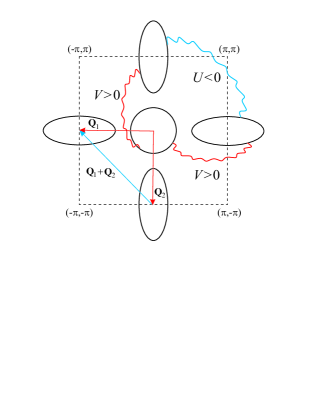
Figure 4: Schematic Fermi surface of the iron pnictides, with a central hole pocket and elliptical electron pockets. The wavy lines represent the inter-pocket pairing interactions generated by the magnetic fluctuations (repulsive $V>0$) and by fluctuations of the vestigial CDW and SVDW states (attractive $U<0$).

III.2 Impact on the superconducting state

Fluctuations of the SVDW and CDW states arise from four-spin correlations, and are complementary to the magnetic fluctuations that arise from two-spin correlations. An important issue is whether these fluctuation modes promote compatible superconducting states. Because the magnetic fluctuations are peaked at momenta $\mathbf{Q}_{1}=\left(\pi,0\right)$ and $\mathbf{Q}_{2}=\left(0,\pi\right)$, they promote a repulsive inter-pocket interaction $V>0$ between the hole and the electron pockets (see Fig. 4). Solution of the corresponding linearized gap equations yields the so-called $s^{+-}$ state, where the gap functions have different signs in the electron and in the hole pockets reviews_pairing . The transition temperature is given by $T_{c}\propto\exp\left(-\frac{1}{\Lambda_{0}}\right)$, with $\Lambda_{0}=\sqrt{2N_{h}N_{e}}\ V$, and $N_{a}$ denoting the density of states of band $a$.

The SVDW and CDW fluctuations, on the other hand, are peaked at the momentum $\mathbf{Q}_{1}+\mathbf{Q}_{2}=\left(\pi,\pi\right)$ and promote an attractive inter-pocket interaction $U<0$ between the two electron pockets (see Fig. 4 and Appendix C). Solution of the linearized gap equation reveals that the leading eigenstate remains the $s^{+-}$ one, but the eigenvalue is enhanced, $\Lambda=\sqrt{\Lambda_{0}^{2}+\Lambda_{U}^{2}}+\Lambda_{U}$, with $\Lambda_{U}=\frac{N_{e}\left|U\right|}{2}>0$. Therefore, fluctuations associated with these vestigial states may enhance the value of $T_{c}$ promoted by spin-fluctuations pairing, without affecting the symmetry of the Cooper pair wave-function. Similar conclusions have been found for the combination of pairing promoted by nematic fluctuations (peaked at $\mathbf{Q}=0$) and magnetic fluctuations (peaked at $\mathbf{Q}_{1}$ and $\mathbf{Q}_{2}$) Lederer14 .

IV Concluding remarks

In summary, we showed that both biaxial tetragonal magnetic ground states of the pnictides – the non-uniform CSDW and non-collinear SVC states – can melt in two-stage processes, giving rise to CDW and SVDW vestigial states, respectively. While both preserve the point-group and time-reversal symmetries, but break the translational symmetry of the iron square lattice, only the SVDW state also breaks inversion symmetry by entangling the spin-space handedness to a doubling of the real-space unit cell. Because in the iron superconductors the hybridization with the puckered As atoms already doubles the unit cell of the Fe square lattice, the CDW and SVDW states are more rigorously classified as intra-unit-cell orders. Recent experiments on $\mathrm{Sr_{1-x}Na_{x}Fe_{2}As_{2}}$ Allred15 and $\mathrm{Ba_{1-x}K_{x}Fe_{2}As_{2}}$ Mallet15 found direct evidence for a low-temperature CSDW phase, which can support a CDW vestigial phase. It remains to be seen whether the tetragonal magnetic phase can be reached in these compounds without first crossing the stripe magnetic state. In contrast, in $\text{Ba}(\text{Fe}_{1-x}\text{Mn}_{x})_{2}\text{As}_{2}$ Kim10 , the tetragonal magnetic phase has been reported to exist over a wide doping range as the primary instability of the paramagnetic phase.

Beyond the physics of iron-based superconductors, our results establish the melting of double-Q orders as a microscopic mechanism to create $d$-density wave states. The latter have been proposed to be realized in other strongly correlated systems, such as the pseudogap phase of underdoped cuprates Chakravarty01 and the hidden-order phase of the heavy fermion compound $\mathrm{URu_{2}Si_{2}}$ Fujimoto11 ; Chakravarty14 ; Blumberg15 , mostly on phenomenological basis. Whether our mechanism is directly applicable to those systems is an appealing topic for future investigation.

Appendix A Saddle-point equations for the SVDW order

We start with the effective action for the magnetic order parameters:

$$S\left[\mathbf{M}_{i}\right]=\int_{q}\chi_{q}^{-1}\left(M_{1}^{2}+M_{2}^{2}\right)+\frac{u}{2}\int_{x}\left(M_{1}^{2}+M_{2}^{2}\right)^{2}-\frac{g}{2}\int_{x}\left(M_{1}^{2}-M_{2}^{2}\right)^{2}+2w\int_{x}\left(\mathbf{M}_{1}\cdot\mathbf{M}_{2}\right)^{2}$$ (4)

where $\int_{q}\equiv T\sum_{\omega_{n}}\int\frac{d^{d}q}{\left(2\pi\right)^{d}}$ and $\int_{x}\equiv\int_{0}^{\beta}d\tau\int d^{d}x$. To proceed, we use the identity:

$$\left(\mathbf{M}_{1}\cdot\mathbf{M}_{2}\right)^{2}=\frac{1}{4}\left(M_{1}^{2}+M_{2}^{2}\right)^{2}-\frac{1}{4}\left(M_{1}^{2}-M_{2}^{2}\right)^{2}-\left(\mathbf{M}_{1}\times\mathbf{M}_{2}\right)^{2}$$ (5)

yielding:

$$S\left[\mathbf{M}_{i}\right]=\int_{q}\chi_{q}^{-1}\left(M_{1}^{2}+M_{2}^{2}\right)+\frac{\left(u+w\right)}{2}\int_{x}\left(M_{1}^{2}+M_{2}^{2}\right)^{2}-\frac{\left(g+w\right)}{2}\int_{x}\left(M_{1}^{2}-M_{2}^{2}\right)^{2}-2w\int_{x}\left(\mathbf{M}_{1}\times\mathbf{M}_{2}\right)^{2}$$ (6)

Hereafter for simplicity we introduce the parameters $\tilde{g}=g+w$ and $\tilde{u}=u+w$. Since we are interested in the vestigial phase of the spin vortex-crystal, which has tetragonal symmetry, the nematic order parameter $\left\langle M_{1}^{2}\right\rangle-\left\langle M_{2}^{2}\right\rangle$ never condenses, and we can ignore the corresponding quartic term. Introducing the Hubbard-Stratonovich fields corresponding to the other two quadratic terms, we obtain:

$$\mathrm{e}^{-\frac{u}{2}\left(M_{1}^{2}+M_{2}^{2}\right)^{2}} = \mathcal{N}\int d\psi\,\mathrm{e}^{\frac{\psi^{2}}{2u}-\psi\left(M_{1}^{2}+M_{2}^{2}\right)}$$

$$\mathrm{e}^{2w\left(\mathbf{M}_{1}\times\mathbf{M}_{2}\right)\cdot\left(\mathbf{M}_{1}\times\mathbf{M}_{2}\right)} = \mathcal{N}\int d\boldsymbol{\varphi}_{\mathrm{SVDW}}\,\mathrm{e}^{\frac{-\varphi^{2}}{2w}+2\boldsymbol{\varphi}_{\mathrm{SVDW}}\cdot\left(\mathbf{M}_{1}\times\mathbf{M}_{2}\right)}$$ (7)

Here, $\boldsymbol{\varphi}_{\mathrm{SVDW}}$ is the spin-vorticity density-wave (SVDW) vectorial order parameter whose mean value is given by $\left\langle\boldsymbol{\varphi}_{\mathrm{SVDW}}\right\rangle=2w\left\langle\mathbf{M}_{1}\times\mathbf{M}_{2}\right\rangle$. The field $\psi$ is not an order parameter, and just renormalizes the magnetic correlation length via $\left\langle\psi\right\rangle=\tilde{u}\left(\left\langle M_{1}^{2}\right\rangle+\left\langle M_{2}^{2}\right\rangle\right)$, i.e. it corresponds to Gaussian magnetic fluctuations. Thus, the effective action is given by:

$$S\left[\mathbf{M}_{i},\psi,\boldsymbol{\varphi}_{\mathrm{SVDW}}\right]=\int_{q}\left(\chi_{q}^{-1}+\psi\right)\left(M_{1}^{2}+M_{2}^{2}\right)-2\int_{x}\boldsymbol{\varphi}_{\mathrm{SVDW}}\cdot\left(\mathbf{M}_{1}\times\mathbf{M}_{2}\right)+\frac{\varphi_{\mathrm{SVDW}}^{2}}{2w}-\frac{\psi^{2}}{2\tilde{u}}$$ (8)

Approaching the SVDW phase from the paramagnetic state, we can integrate out the magnetic degrees of freedom, yielding an effective action for $\psi$ and $\boldsymbol{\varphi}_{\mathrm{SVDW}}$:

$$S_{\mathrm{eff}}\left[\psi,\boldsymbol{\varphi}_{\mathrm{SVDW}}\right]=\frac{\varphi_{\mathrm{SVDW}}^{2}}{2w}-\frac{\psi^{2}}{2\tilde{u}}+\frac{1}{2}\int_{q}\log\left(\prod_{i}\lambda_{i,q}\right)$$ (9)

where $\lambda_{i,q}$ are the eigenvalues of the matrix $A_{ij}$ corresponding to the Gaussian action in $\mathbf{M}_{i}$. The Gaussian part of the action can be rewritten in the convenient matrix form:

$$\left(\begin{array}[]{cc}\mathbf{M}_{1}&\mathbf{M}_{2}\end{array}\right)\left(\begin{array}[]{cccccc}\chi_{q}^{-1}+\psi&0&0&0&-\varphi_{z}&\varphi_{y}\\ 0&\chi_{q}^{-1}+\psi&0&\varphi_{z}&0&-\varphi_{x}\\ 0&0&\chi_{q}^{-1}+\psi&-\varphi_{y}&\varphi_{x}&0\\ 0&\varphi_{z}&-\varphi_{y}&\chi_{q}^{-1}+\psi&0&0\\ -\varphi_{z}&0&\varphi_{x}&0&\chi_{q}^{-1}+\psi&0\\ \varphi_{y}&-\varphi_{x}&0&0&0&\chi_{q}^{-1}+\psi\end{array}\right)\left(\begin{array}[]{c}\mathbf{M}_{1}\\ \mathbf{M}_{2}\end{array}\right)$$ (10)

Evaluation of the eigenvalues gives:

$$S_{\mathrm{eff}}\left[\psi,\boldsymbol{\varphi}_{\mathrm{SVDW}}\right]=\frac{\varphi_{\mathrm{SVDW}}^{2}}{2w}-\frac{\psi^{2}}{2\tilde{u}}+\int_{q}\log\left[\left(\chi_{q}^{-1}+\psi\right)\left(\chi_{q}^{-1}+\psi+\varphi_{\mathrm{SVDW}}\right)\left(\chi_{q}^{-1}+\psi-\varphi_{\mathrm{SVDW}}\right)\right]$$ (11)

So far our result is exact. To proceed, we employ the saddle-point approximation to determine the equations of state for $\psi$ and $\varphi_{\mathrm{SVDW}}$, which corresponds to self-consistently accounting for the Gaussian magnetic fluctuations. The saddle-point equations become:

$$\frac{\varphi_{\mathrm{SVDW}}}{w} = \int_{q}\frac{1}{\chi_{q}^{-1}+\psi-\varphi_{\mathrm{SVDW}}}-\int_{q}\frac{1}{\chi_{q}^{-1}+\psi+\varphi_{\mathrm{SVDW}}}$$

$$\frac{\psi}{\tilde{u}} = \int_{q}\frac{1}{\chi_{q}^{-1}+\psi-\varphi_{\mathrm{SVDW}}}+\int_{q}\frac{1}{\chi_{q}^{-1}+\psi+\varphi_{\mathrm{SVDW}}}+\int_{q}\frac{1}{\chi_{q}^{-1}+\psi}$$ (12)

Since our focus is on the proximity to a finite-temperature magnetic transition, we ignore the spin dynamics and use the low-energy expansion for the spin susceptibility appropriate for anisotropic layered systems:

$$\chi_{q}^{-1}=r_{0}+q_{\parallel}^{2}+J_{z}\sin^{2}\frac{q_{z}}{2}$$ (13)

where $r_{0}=a\left(T-T_{N}\right)$, $a>0$, $T_{N}$ is the mean-field magnetic transition temperature, $q_{\parallel}^{2}=q_{x}^{2}+q_{y}^{2}$, and $J_{z}$ is the inter-layer magnetic coupling. Defining the renormalized magnetic mass:

$$r=r_{0}+\psi\propto\xi^{-2}$$ (14)

where $\xi$ is the magnetic correlation length, we obtain:

$$\varphi_{\mathrm{SVDW}} = w\left[\int_{q}\frac{1}{r+q_{\parallel}^{2}+J_{z}\sin^{2}\frac{q_{z}}{2}-\varphi_{\mathrm{SVDW}}}-\int_{q}\frac{1}{r+q_{\parallel}^{2}+J_{z}\sin^{2}\frac{q_{z}}{2}+\varphi_{\mathrm{SVDW}}}\right]$$ (15)

$$r = r_{0}+\tilde{u}\left[\int_{q}\frac{1}{r+q_{\parallel}^{2}+J_{z}\sin^{2}\frac{q_{z}}{2}-\varphi_{\mathrm{SVDW}}}+\int_{q}\frac{1}{r+q_{\parallel}^{2}+J_{z}\sin^{2}\frac{q_{z}}{2}+\varphi_{\mathrm{SVDW}}}+\int_{q}\frac{1}{r+q_{\parallel}^{2}+J_{z}\sin^{2}\frac{q_{z}}{2}}\right]$$

The integrals can be evaluated in a straightforward way (we consider only the $\omega_{n}=0$ contribution to the sum over Matsubara frequencies, since we are interested in the finite temperature transition):

$$\int_{q}\frac{1}{q_{\parallel}^{2}+J_{z}\sin^{2}\frac{q_{z}}{2}+a} = \frac{T_{N}}{4\pi}\int_{0}^{2\pi}\frac{dq_{z}}{2\pi}\int_{J_{z}\sin^{2}\frac{q_{z}}{2}+a}^{\Lambda^{2}}\frac{dx}{x}$$ (16)

$$= \frac{T_{N}}{4\pi}\int_{0}^{2\pi}\frac{dq_{z}}{2\pi}\ln\left(\frac{\Lambda^{2}}{J_{z}\sin^{2}\frac{q_{z}}{2}+a}\right)$$

$$= \frac{T_{N}}{2\pi}\left[\ln 2\Lambda-\ln\left(\sqrt{J_{z}+a}+\sqrt{a}\right)\right]$$

Defining the renormalized critical temperature $\tilde{r}_{0}=a(T-\tilde{T}_{N})$ via:

$$\tilde{r}_{0}=r_{0}+\frac{3\tilde{u}T_{N}}{2\pi}\ln\frac{2\Lambda}{\sqrt{J_{z}}}$$ (17)

we obtain the self-consistent equations:

$$\varphi_{\mathrm{SVDW}} = \frac{wT_{N}}{2\pi}\ln\frac{\sqrt{J_{z}+r+\varphi_{\mathrm{SVDW}}}+\sqrt{r+\varphi_{\mathrm{SVDW}}}}{\sqrt{J_{z}+r-\varphi_{\mathrm{SVDW}}}+\sqrt{r-\varphi_{\mathrm{SVDW}}}}$$ (18)

$$r = \tilde{r}_{0}-\frac{\tilde{u}T_{N}}{2\pi}\ln\left[\frac{\left(\sqrt{J_{z}+r+\varphi_{\mathrm{SVDW}}}+\sqrt{r+\varphi_{\mathrm{SVDW}}}\right)\left(\sqrt{J_{z}+r-\varphi_{\mathrm{SVDW}}}+\sqrt{r-\varphi_{\mathrm{SVDW}}}\right)\left(\sqrt{J_{z}+r}+\sqrt{r}\right)}{J_{z}^{3/2}}\right]$$

For simplicity, we define the renormalized parameters $\left(\bar{w},\bar{u}\right)\equiv\left(w,u\right)\frac{T_{N}}{2\pi}$ as well as $\alpha\equiv\frac{\tilde{u}}{w}=\frac{u}{w}+1$ and $\tilde{J}_{z}\equiv J_{z}/\bar{w}$. Then the equations can be written as:

$$\varphi_{\mathrm{SVDW}} = \ln\frac{\sqrt{\tilde{J}_{z}+r+\varphi_{\mathrm{SVDW}}}+\sqrt{r+\varphi_{\mathrm{SVDW}}}}{\sqrt{\tilde{J}_{z}+r-\varphi_{\mathrm{SVDW}}}+\sqrt{r-\varphi_{\mathrm{SVDW}}}}$$ (19)

$$r = \tilde{r}_{0}-\alpha\ln\left[\frac{\left(\sqrt{\tilde{J}_{z}+r+\varphi_{\mathrm{SVDW}}}+\sqrt{r+\varphi_{\mathrm{SVDW}}}\right)\left(\sqrt{\tilde{J}_{z}+r-\varphi_{\mathrm{SVDW}}}+\sqrt{r-\varphi_{\mathrm{SVDW}}}\right)\left(\sqrt{\tilde{J}_{z}+r}+\sqrt{r}\right)}{\tilde{J}_{z}^{3/2}}\right]$$

where $r$, $\tilde{r}_{0}$, and $\varphi_{\mathrm{SVDW}}$ were rescaled by $\bar{w}$ as well. The SVDW transition temperature can be obtained by linearizing the equations around $\varphi_{\mathrm{SVDW}}=0$. From the first equation, we obtain the correlation length $r_{1}$ at the SVDW transition:

$$r_{1}=\frac{\sqrt{\tilde{J}_{z}^{2}+4}-\tilde{J}_{z}}{2}$$ (20)

which, when substituted in the second equation, gives the SVDW transition temperature $\tilde{r}_{0,\mathrm{SVDW}}$:

$$\tilde{r}_{0,\mathrm{SVDW}}=\frac{\sqrt{\tilde{J}_{z}^{2}+4}-\tilde{J}_{z}}{2}+3\alpha\ln\left(\frac{\sqrt{\sqrt{\tilde{J}_{z}^{2}+4}+\tilde{J}_{z}}+\sqrt{\sqrt{\tilde{J}_{z}^{2}+4}-\tilde{J}_{z}}}{\sqrt{2\tilde{J_{z}}}}\right)$$ (21)

The magnetic transition temperature $\tilde{r}_{0,\mathrm{mag}}$ is signaled by the vanishing of the renormalized magnetic mass, i.e. the lowest eigenvalue of the Eq. (10), $r-\varphi_{\mathrm{SVDW}}$. Therefore, it takes place when $r$ reaches the value $r_{2}$ determined implicitly by:

$$r_{2}=\ln\frac{\sqrt{\tilde{J}_{z}+2r_{2}}+\sqrt{2r_{2}}}{\sqrt{\tilde{J}_{z}}}$$ (22)

The magnetic transition temperature is therefore given by:

$$\tilde{r}_{0,\mathrm{mag}}=r_{2}\left(1+\alpha\right)+\alpha\ln\left[\frac{\sqrt{\tilde{J}_{z}+r_{2}}+\sqrt{r_{2}}}{\sqrt{\tilde{J}_{z}}}\right]$$ (23)

The SVDW and magnetic transitions are split when $\tilde{r}_{0,\mathrm{SVDW}}>\tilde{r}_{0,\mathrm{mag}}$. The region in the $\left(\frac{u}{w},\tilde{J_{z}}\right)$ parameter space where this condition is satisfied corresponds to the shaded area of Fig. 3 in the main text (recall that $\frac{u}{w}=\alpha-1$).

To determine the character of the SVDW transition, we can expand $\tilde{r}_{0}$ for small $\varphi_{\mathrm{SVDW}}$. Substituting $r=r_{1}+a\varphi_{\mathrm{SVDW}}^{2}$ in the first equation of (19) and expanding for small $\varphi_{\mathrm{SVDW}}$ gives the coefficient of the quadratic term:

$$a=\frac{8+3\tilde{J}_{z}^{2}}{12\sqrt{\tilde{J}_{z}^{2}+4}}$$ (24)

Substituting it in the second equation of (19) and collecting the quadratic terms in $\varphi_{\mathrm{SVDW}}$ yields:

$$\tilde{r}_{0}\left(\varphi_{\mathrm{SVDW}}\right)\approx\tilde{r}_{0,\mathrm{SVDW}}+\left[\frac{16+3\tilde{J}_{z}^{2}\left(2+\alpha\right)}{24\sqrt{\tilde{J}_{z}^{2}+4}}\right]\varphi_{\mathrm{SVDW}}^{2}$$ (25)

Therefore, because the coefficient is always positive, the solution with $\varphi_{\mathrm{SVDW}}\neq 0$ is achieved at a larger temperature than the solution with $\varphi_{\mathrm{SVDW}}=0$, in other words, $\tilde{r}_{0}\left(\varphi_{\mathrm{SVDW}}>0\right)>\tilde{r}_{0}\left(\varphi_{\mathrm{SVDW}}\rightarrow 0\right)$. As a result, the SVDW transition is first-order within the saddle-point approximation, even when it is split from the magnetic transition.

Appendix B Derivation of the Ginzburg-Landau free energy

Our starting point is a 3-band model with a circular hole pocket $h$ centered at $\left(0,0\right)$ and two elliptical electron pockets $e_{1,2}$ centered at $\mathbf{Q}_{1}=\left(\pi,0\right)$ and $\mathbf{Q}_{2}=\left(0,\pi\right)$, respectively. The band dispersions can be conveniently parametrized by Fernandes12 :

$$\xi_{h,\mathbf{k}} = -\xi_{\mathbf{k}}=-\frac{k^{2}}{2m}+\varepsilon_{0}$$

$$\xi_{e_{1},\mathbf{k}+\mathbf{Q}_{1}} = \xi_{\mathbf{k}}-\left(\delta_{0}+\delta_{2}\cos 2\theta\right)$$

$$\xi_{e_{2},\mathbf{k}+\mathbf{Q}_{2}} = \xi_{\mathbf{k}}-\left(\delta_{0}-\delta_{2}\cos 2\theta\right)$$ (26)

Here, $\delta_{0}$ is proportional to the chemical potential and $\delta_{2}$ to the ellipticity of the electron pockets. The angle $\theta$ is measured relative to the $k_{x}$ axis. The non-interacting Hamiltonian is therefore given by (hereafter sums over repeated spin indices are implicitly assumed):

$$H_{0}=\sum_{\mathbf{k}}\xi_{h,\mathbf{k}}c_{h,\mathbf{k}\sigma}^{\dagger}c_{h,\mathbf{k}\sigma}+\sum_{\mathbf{k}}\xi_{e_{1},\mathbf{k}}c_{e_{1},\mathbf{k}\sigma}^{\dagger}c_{e_{1},\mathbf{k}\sigma}+\sum_{\mathbf{k}}\xi_{e_{2},\mathbf{k}}c_{e_{2},\mathbf{k}\sigma}^{\dagger}c_{e_{2},\mathbf{k}\sigma}$$ (27)

These electronic states couple to the magnetic order parameters $\mathbf{M}_{1}$ and $\mathbf{M}_{2}$ according to:

$$H_{\mathrm{mag}}=\sum_{\mathbf{k},i}\mathbf{M}_{i}\cdot\left(c_{e_{i},\mathbf{k}\alpha}^{\dagger}\boldsymbol{\sigma}_{\alpha\beta}c_{h,\mathbf{k}\beta}+\mathrm{h.c.}\right)$$ (28)

In principle, this last term can be obtained via a Hubbard-Stratonovich transformation of the original interaction terms projected into the magnetic channel, as shown in Ref. Fernandes12 . Here, because we are interested in the higher-order couplings of the action involving the $\mathbf{M}_{i}$ order parameters, we neglect these interaction terms, since they only affect the quadratic terms of the action.

B.1 Absence of magnetic field

In the case where there is no external magnetic field, we focus on the two types of fermionic order that couple directly to the SVDW order parameter, $\mathbf{M}_{1}\times\mathbf{M}_{2}$, and to the CDW order parameter $\mathbf{M}_{1}\cdot\mathbf{M}_{2}$. Thus, we introduce the $\mathbf{Q}_{1}+\mathbf{Q}_{2}=\left(\pi,\pi\right)$ spin-current density-wave $\boldsymbol{\Delta}^{\prime\prime}_{S}$ (i.e. a purely imaginary SDW) and the checkerboard charge order $\Delta^{\prime}_{C}$ (i.e. a purely real CDW) defined by:

$$\mathcal{H}_{iS} =i\sum_{\mathbf{k}}\boldsymbol{\Delta}^{\prime\prime}_{S}\cdot\boldsymbol{\sigma}_{\alpha\beta}^{\phantom{\dagger}}\left(c_{e_{2},\mathbf{k}\alpha}^{\dagger}c_{e_{1},\mathbf{k}\beta}^{\phantom{\dagger}}-c_{e_{1},\mathbf{k}\alpha}^{\dagger}c_{e_{2},\mathbf{k}\beta}^{\phantom{\dagger}}\right)$$

$$\mathcal{H}_{C} =\sum_{\mathbf{k}}\Delta^{\prime}_{C}\delta_{\alpha\beta}\left(c_{e_{2},\mathbf{k}\alpha}^{\dagger}c_{e_{1},\mathbf{k}\beta}^{\phantom{\dagger}}+c_{e_{1},\mathbf{k}\alpha}^{\dagger}c_{e_{2},\mathbf{k}\beta}^{\phantom{\dagger}}\right)$$ (29)

To proceed, we introduce the $6$-dimensional Nambu operator:

$$\Psi_{\mathbf{k}}^{\dagger}=\left(\begin{array}[]{cccccc}c_{h,\mathbf{k}\uparrow}^{\dagger}&c_{h,\mathbf{k}\downarrow}^{\dagger}&c_{e_{1},\mathbf{k}\uparrow}^{\dagger}&c_{e_{1},\mathbf{k}\downarrow}^{\dagger}&c_{e_{2},\mathbf{k}\uparrow}^{\dagger}&c_{e_{2},\mathbf{k}\downarrow}^{\dagger}\end{array}\right)$$ (30)

which allows us to write the fermionic action in the compact form:

$$S=-\int_{k}\Psi_{k}^{\dagger}\hat{\mathcal{G}}_{k}^{-1}\Psi_{k}+S_{0}\left[M_{i}^{2}\right]$$ (31)

In the previous expression, $S_{0}\left[M_{i}^{2}\right]$ corresponds to the terms $M_{i}^{2}$ that arise from the decoupling of the fermionic interactions. As we explained above, these terms can be ignored for our purposes. The total Green’s function is given by:

$$\hat{\mathcal{G}}_{k}^{-1}=\left(\hat{\mathcal{G}}_{k}^{(0)}\right)^{-1}-\hat{V}_{\mathrm{mag}}-\hat{V}_{iS}-\hat{V}_{C}$$ (32)

The bare part is:

$$\hat{\mathcal{G}}_{k}^{(0)}=\left(\begin{array}[]{cccccc}G_{h,k}&0&0&0&0&0\\ 0&G_{h,k}&0&0&0&0\\ 0&0&G_{e_{1},k}&0&0&0\\ 0&0&0&G_{e_{1},k}&0&0\\ 0&0&0&0&G_{e_{2},k}&0\\ 0&0&0&0&0&G_{e_{2},k}\end{array}\right)$$ (33)

where $G_{i,k}^{-1}=i\omega_{n}-\xi_{i,\mathbf{k}}$ are the non-interacting single-particle Green’s functions. The interacting parts are:

$$\hat{V}_{\mathrm{mag}}=\left(\begin{array}[]{cccccc}0&0&-M_{1,z}&-M_{1,x}+iM_{1,y}&-M_{2,z}&-M_{2,x}+iM_{2,y}\\ 0&0&-M_{1,x}-iM_{1,y}&M_{1,z}&-M_{2,x}-iM_{2,y}&M_{2,z}\\ -M_{1,z}&-M_{1,x}+iM_{1,y}&0&0&0&0\\ -M_{1,x}-iM_{1,y}&M_{1,z}&0&0&0&0\\ -M_{2,z}&-M_{2,x}+iM_{2,y}&0&0&0&0\\ -M_{2,x}-iM_{2,y}&M_{2,z}&0&0&0&0\end{array}\right)$$ (34)

and:

$$\hat{V}_{iS}=\left(\begin{array}[]{cccccc}0&0&0&0&0&0\\ 0&0&0&0&0&0\\ 0&0&0&0&i\Delta^{\prime\prime}_{S,z}&i\left(\Delta^{\prime\prime}_{S,x}-i\Delta^{\prime\prime}_{S,y}\right)\\ 0&0&0&0&i\left(\Delta^{\prime\prime}_{S,x}+i\Delta^{\prime\prime}_{S,y}\right)&-i\Delta^{\prime\prime}_{S,z}\\ 0&0&-i\Delta^{\prime\prime}_{S,z}&-i\left(\Delta^{\prime\prime}_{S,x}-i\Delta^{\prime\prime}_{S,y}\right)&0&0\\ 0&0&-i\left(\Delta^{\prime\prime}_{S,x}+i\Delta^{\prime\prime}_{S,y}\right)&i\Delta^{\prime\prime}_{S,z}&0&0\end{array}\right)$$ (35)

as well as:

$$\hat{V}_{C}=\left(\begin{array}[]{cccccc}0&0&0&0&0&0\\ 0&0&0&0&0&0\\ 0&0&0&0&-\Delta^{\prime}_{C}&0\\ 0&0&0&0&0&-\Delta^{\prime}_{C}\\ 0&0&-\Delta^{\prime}_{C}&0&0&0\\ 0&0&0&-\Delta^{\prime}_{C}&0&0\end{array}\right)$$ (36)

It is now straightforward to integrate out the fermions and obtain the effective magnetic action:

$$S_{\mathrm{eff}}\left[\mathbf{M}_{1},\mathbf{M}_{2},\boldsymbol{\Delta}^{\prime\prime}_{S},\Delta^{\prime}_{C}\right]=-\mathrm{Tr}\ln\left[1-\hat{\mathcal{G}}_{0}\left(\hat{V}_{\mathrm{mag}}+\hat{V}_{iS}+\hat{V}_{C}\right)\right]\approx\sum_{n}\frac{1}{n}\mathrm{Tr}\left[\hat{\mathcal{G}}_{0}\left(\hat{V}_{\mathrm{mag}}+\hat{V}_{iS}+\hat{V}_{C}\right)\right]^{n}$$ (37)

where, in the last step, we expanded for small $M_{1}$, $M_{2}$. Here, $\mathrm{Tr}\left(\cdots\right)$ refers to sum over momentum, frequency and Nambu indices. A straightforward evaluation gives, to leading order in the coupling between $\boldsymbol{\Delta}^{\prime\prime}_{S}$, $\Delta^{\prime}_{C}$, and $\mathbf{M}_{i}$:

$$S_{\mathrm{eff}}\left[\mathbf{M}_{1},\mathbf{M}_{2},\boldsymbol{\Delta}^{\prime\prime}_{S},\Delta^{\prime}_{C}\right]=S\left[\mathbf{M}_{1},\mathbf{M}_{2}\right]+\lambda\boldsymbol{\Delta}^{\prime\prime}_{S}\cdot\left(\mathbf{M}_{1}\times\mathbf{M}_{2}\right)-\lambda\Delta^{\prime}_{C}\left(\mathbf{M}_{1}\cdot\mathbf{M}_{2}\right)$$ (38)

with the coefficient:

$$\lambda=4\int_{k}G_{h,k}G_{e_{1},k}G_{e_{2},k}$$ (39)

For perfect nesting, $\delta_{0}=\delta_{2}=0$, this coefficient vanishes. For a system in proximity to a finite temperature phase transition, expansion in powers of $\delta_{0}$ gives:

$$\lambda \approx 4\rho_{F}T\sum_{n}\int d\xi\frac{1}{\left(i\omega_{n}+\xi\right)}\frac{1}{\left(i\omega_{n}-\xi+\delta_{0}\right)^{2}}$$

$$\lambda \approx -8\delta_{0}\rho_{F}T\sum_{n}\int d\xi\frac{1}{\left(i\omega_{n}+\xi\right)}\frac{1}{\left(i\omega_{n}-\xi\right)^{3}}$$

$$\lambda \approx -\left(\frac{\delta_{0}}{T}\right)\frac{7\zeta\left(3\right)\rho_{F}}{2\pi^{2}T}$$ (40)

where $\rho_{F}$ is the density of states at the Fermi level. Therefore, it is clear that a spin-current density-wave $\boldsymbol{\Delta}^{\prime\prime}_{S}$ parallel to $\boldsymbol{\varphi}_{\mathrm{SVDW}}$ is triggered by the SVDW order parameter, $\boldsymbol{\varphi}_{\mathrm{SVDW}}\propto\mathbf{M}_{1}\times\mathbf{M}_{2}$, whereas a checkerboard charge order $\Delta^{\prime}_{C}$ is triggered by the CDW order parameter $\varphi_{\mathrm{CDW}}\propto\mathbf{M}_{1}\cdot\mathbf{M}_{2}$.

B.2 Non-zero magnetic field

In the presence of a magnetic field, additional types of fermionic order are triggered by the condensation of the SVDW and CDW order parameters. To show that, we first introduce the Zeeman coupling between the uniform field $\mathbf{H}$ and the electrons:

$$H_{\mathrm{Zeeman}}=\sum_{\mathbf{k},i}\mathbf{H}\cdot\boldsymbol{\sigma}_{\alpha\beta}c_{i,\mathbf{k}\alpha}^{\dagger}c_{i,\mathbf{k}\beta}$$ (41)

We also introduce the $\mathbf{Q}_{1}+\mathbf{Q}_{2}=\left(\pi,\pi\right)$ charge-current density-wave $\Delta^{\prime\prime}_{C}$ (i.e. a purely imaginary CDW) and the spin density-wave $\boldsymbol{\Delta}^{\prime}_{S}$ (i.e. a purely real SDW) defined by:

$$\mathcal{H}_{S} =\sum_{\mathbf{k}}\boldsymbol{\Delta}^{\prime}_{S}\cdot\boldsymbol{\sigma}_{\alpha\beta}^{\phantom{\dagger}}\left(c_{e_{2},\mathbf{k}\alpha}^{\dagger}c_{e_{1},\mathbf{k}\beta}^{\phantom{\dagger}}+c_{e_{1},\mathbf{k}\alpha}^{\dagger}c_{e_{2},\mathbf{k}\beta}^{\phantom{\dagger}}\right)$$

$$\mathcal{H}_{iC} =i\sum_{\mathbf{k}}\Delta^{\prime\prime}_{C}\delta_{\alpha\beta}\left(c_{e_{2},\mathbf{k}\alpha}^{\dagger}c_{e_{1},\mathbf{k}\beta}^{\phantom{\dagger}}-c_{e_{1},\mathbf{k}\alpha}^{\dagger}c_{e_{2},\mathbf{k}\beta}^{\phantom{\dagger}}\right)$$ (42)

Following the same steps as in the previous subsection, we obtain the expanded action:

$$S_{\mathrm{eff}}\left[\mathbf{M}_{1},\mathbf{M}_{2},\boldsymbol{\Delta}^{\prime}_{S},\Delta^{\prime\prime}_{C}\right]\approx\sum_{n}\frac{1}{n}\mathrm{Tr}\left[\hat{\mathcal{G}}_{0}\left(\hat{V}_{\mathrm{mag}}+\hat{V}_{S}+\hat{V}_{iC}+\hat{V}_{\mathrm{Zeeman}}\right)\right]^{n}$$ (43)

where the Nambu-space matrices are given by:

$$\hat{V}_{\mathrm{Zeeman}}=\left(\begin{array}[]{cccccc}-H_{z}&-H_{x}+iH_{y}&0&0&0&0\\ -H_{x}-iH_{y}&H_{z}&0&0&0&0\\ 0&0&-H_{z}&-H_{x}+iH_{y}&0&0\\ 0&0&-H_{x}-iH_{y}&h_{z}&0&0\\ 0&0&0&0&-H_{z}&-H_{x}+iH_{y}\\ 0&0&0&0&-H_{x}-iH_{y}&H_{z}\end{array}\right)$$ (44)

and:

$$\hat{V}_{iC}=\left(\begin{array}[]{cccccc}0&0&0&0&0&0\\ 0&0&0&0&0&0\\ 0&0&0&0&i\Delta^{\prime\prime}_{C}&0\\ 0&0&0&0&0&i\Delta^{\prime\prime}_{C}\\ 0&0&-i\Delta^{\prime\prime}_{C}&0&0&0\\ 0&0&0&-i\Delta^{\prime\prime}_{C}&0&0\end{array}\right)$$ (45)

as well as:

$$\hat{V}_{S}=\left(\begin{array}[]{cccccc}0&0&0&0&0&0\\ 0&0&0&0&0&0\\ 0&0&0&0&-\Delta^{\prime}_{S,z}&-\left(\Delta^{\prime}_{S,x}-i\Delta^{\prime}_{S,y}\right)\\ 0&0&0&0&-\left(\Delta^{\prime}_{S,x}+i\Delta^{\prime}_{S,y}\right)&\Delta^{\prime}_{S,z}\\ 0&0&-\Delta^{\prime}_{S,z}&-\left(\Delta^{\prime}_{S,x}-i\Delta^{\prime}_{S,y}\right)&0&0\\ 0&0&-\left(\Delta^{\prime}_{S,x}+i\Delta^{\prime}_{S,y}\right)&\Delta^{\prime}_{S,z}&0&0\end{array}\right)$$ (46)

A straightforward evaluation yields, to leading order in the magnetic field:

$$\mathcal{S}_{\mathrm{eff}} =\mathcal{S}_{\mathrm{eff}}\left[\mathbf{H}=0\right]+\zeta\left[\left(\mathbf{H}\cdot\mathbf{M}_{1}\right)^{2}+\left(\mathbf{H}\cdot\mathbf{M}_{2}\right)^{2}\right]$$ (47)

$$+\gamma\left[\Delta^{\prime\prime}_{C}\mathbf{H}\cdot\left(\mathbf{M}_{1}\times\mathbf{M}_{2}\right)+\left(\mathbf{H}\cdot\boldsymbol{\Delta}^{\prime}_{S}\right)\left(\mathbf{M}_{1}\cdot\mathbf{M}_{2}\right)\right]$$

$$+\eta\left[\left(\mathbf{M}_{1}\cdot\mathbf{H}\right)\left(\mathbf{M}_{2}\cdot\boldsymbol{\Delta}^{\prime}_{S}\right)+\left(\mathbf{M}_{2}\cdot\mathbf{H}\right)\left(\mathbf{M}_{1}\cdot\boldsymbol{\Delta}^{\prime}_{S}\right)\right]$$

where we neglected all isotropic biquadratic terms of the form $H^{2}M_{i}^{2}$. The coefficients are given by:

$$\zeta = 4\int_{k}G_{h,k}^{2}G_{e_{1},k}^{2}$$

$$\gamma = 4\int_{k}G_{h,k}G_{e_{1},k}G_{e_{2},k}\left(G_{e_{1},k}+G_{e_{2},k}-G_{h,k}\right)$$

$$\eta = 4\int_{k}G_{h,k}^{2}G_{e_{1},k}G_{e_{2},k}$$ (48)

It is useful to perform an expansion around perfect nesting, $\delta_{0}=\delta_{2}=0$. The coefficients $\zeta$ and $\eta$ become identical in this limit:

$$\zeta=\eta=\frac{\rho_{F}}{T^{2}}\left(\frac{7\zeta\left(3\right)}{2\pi^{2}}\right)$$ (49)

The fact that $\zeta>0$ implies that the magnetic field induces an easy plane, rather than an easy axis anisotropy. As for the coefficient $\eta$, it remains zero in all orders in perturbation theory if an infinite bandwidth is assumed. However, keeping the top of the hole pocket $W$ (or bottom of the electron pocket) throughout the calculation gives:

$$\gamma\approx\frac{\rho_{F}}{T^{2}}\left(\frac{W}{T}\right)^{-2}$$ (50)

The fact that $\gamma\neq 0$ implies that, in the presence of a uniform field, the SVDW order parameter $\boldsymbol{\varphi}_{\mathrm{SVDW}}\propto\mathbf{M}_{1}\times\mathbf{M}_{2}$ also triggers a charge-current density-wave $\Delta^{\prime\prime}_{C}$, whereas the CDW order parameter $\varphi_{\mathrm{CDW}}\propto\mathbf{M}_{1}\cdot\mathbf{M}_{2}$ triggers a spin density-wave of same period, $\boldsymbol{\Delta}^{\prime}_{S}$. Although this was expected by symmetry, here we have microscopic expressions for the corresponding Ginzburg-Landau coefficients. It is interesting then to compare the coefficient $\gamma$ in Eq. (47), which determines the amplitudes of $\Delta^{\prime\prime}_{C}$ and $\boldsymbol{\Delta}^{\prime}_{S}$, to the coefficient $\lambda$ in Eq. (38), which determines the amplitudes of $\boldsymbol{\Delta}^{\prime\prime}_{S}$ and $\Delta^{\prime}_{C}$. We find that:

$$\frac{\gamma H}{\lambda}\approx-2.3\left(\frac{T^{2}H}{W^{2}\delta_{0}}\right)$$ (51)

Therefore, for pnictides whose band dispersions do not deviate strongly from perfect nesting, and whose bandwidths are not too large either, it is conceivable that the two coupling constants $\gamma H$ and $\lambda$ will be of similar order for moderate values of the magnetic field $H$. As a result, the charge-current density-wave and the spin density-wave generated in the presence of the field could be as large as the spin-current density-wave and the charge density-wave generated in the absence of the field.

Appendix C Superconducting pairing interactions

Here we show explicitly that fluctuations associated with an imaginary SDW instability or with a real CDW instability give rise to attractive pairing interactions. For our purposes, it is sufficient to consider only the two Fermi pockets connected by the momentum transfer $\mathbf{Q}=\left(\pi,\pi\right)$ associated with these two ordered states. To simplify the notation, here we will denote the fermionic operators associated with these bands by $d_{\mathbf{k}\sigma}$ and $f_{\mathbf{k}\sigma}$. In both cases, $\mathbf{k}$ is measured relative to the center of each Fermi pocket. Consider first the action describing the coupling between the electrons and the complex SDW bosonic field $\boldsymbol{\Delta}_{S}=\Delta_{S}\hat{\mathbf{z}}$ (for simplicity, we consider it polarized along the $z$ axis):

$$S = -\int_{k}\left[\left(i\omega_{n}-\varepsilon_{d,\mathbf{k}}\right)d_{\mathbf{k}\sigma}^{\dagger}d_{\mathbf{k}\sigma}+\left(i\omega_{n}-\varepsilon_{f,\mathbf{k}}\right)f_{\mathbf{k}\sigma}^{\dagger}f_{\mathbf{k}\sigma}\right]+g\int_{k,q}\sigma\left(\Delta^{\prime}_{S,-k-q}d_{\mathbf{k}\sigma}^{\dagger}f_{\mathbf{q}\sigma}+\Delta^{\prime}_{S,-k-q}f_{\mathbf{k}\sigma}^{\dagger}d_{\mathbf{q}\sigma}\right)$$ (52)

$$+g\int_{k,q}\sigma\left(i\Delta^{\prime\prime}_{S,-k-q}d_{\mathbf{k}\sigma}^{\dagger}f_{\mathbf{q}\sigma}-i\Delta^{\prime\prime}_{S,-k-q}f_{\mathbf{k}\sigma}^{\dagger}d_{\mathbf{q}\sigma}\right)$$

$$+\int_{k}\chi_{S}^{-1}\left(\mathbf{k},\Omega_{n}\right)\Delta^{\prime}_{S,k}\Delta^{\prime}_{S,-k}+\int_{k}\chi_{iS}^{-1}\left(\mathbf{k},\Omega_{n}\right)\Delta^{\prime\prime}_{S,k}\Delta^{\prime\prime}_{S,-k}$$

where $k\equiv\left(\mathbf{k},\omega_{n}\right)$, $\int_{k}\equiv T\sum\limits_{n}\int\frac{d^{d}k}{\left(2\pi\right)^{d}}$ (with the appropriate bosonic $\Omega_{n}$ or fermionic $\omega_{n}$ Matsubara frequency), and we left implicit the sum over spin indices, as well as the dependence of the fermionic operators on the fermionic Matsubara frequencies. $\chi_{S}$ and $\chi_{iS}$ are the susceptibilities associated with the real and imaginary SDW, and $g$ is the coupling constant. Note that, because $\mathbf{Q}$ is a commensurate vector, the real and imaginary SDW fields are independent. Introducing the four-dimensional Nambu operator:

$$\Psi_{\mathbf{k}}^{\dagger}=\left(\begin{array}[]{cccc}d_{\mathbf{k}\uparrow}^{\dagger}&d_{-\mathbf{k}\downarrow}&f_{\mathbf{k}\uparrow}^{\dagger}&f_{-\mathbf{k}\downarrow}\end{array}\right)$$ (53)

the action can be written conveniently as:

$$S = -\int_{k}\Psi_{\mathbf{k}}^{\dagger}\left(i\omega_{n}\hat{1}-\hat{\varepsilon}_{\mathbf{k}}\right)\Psi_{\mathbf{k}}+\int_{k}\chi_{S}^{-1}\left(\mathbf{k},\Omega_{n}\right)\Delta^{\prime}_{S,k}\Delta^{\prime}_{S,-k}+\int_{k}\chi_{iS}^{-1}\left(\mathbf{k},\Omega_{n}\right)\Delta^{\prime\prime}_{S,k}\Delta^{\prime\prime}_{S,-k}$$ (54)

$$+g\int_{k,q}\Delta^{\prime}_{S,-k-q}\Psi_{\mathbf{k}}^{\dagger}\hat{\rho}_{S}\Psi_{\mathbf{p}}+g\int_{k,q}\Delta^{\prime\prime}_{S,-k-q}\Psi_{\mathbf{k}}^{\dagger}\hat{\rho}_{iS}\Psi_{\mathbf{p}}$$

where we defined the $4\times 4$ matrices:

$$\hat{\varepsilon}_{\mathbf{k}}=\left(\begin{array}[]{cc}\varepsilon_{d,\mathbf{k}}\tau_{z}&0\\ 0&\varepsilon_{f,\mathbf{k}}\tau_{z}\end{array}\right)\>;\;\;\hat{\rho}_{S}=\left(\begin{array}[]{cc}0&\tau_{0}\\ \tau_{0}&0\end{array}\right)\equiv\tau_{0}\otimes\sigma_{x}\>;\;\;\hat{\rho}_{iS}=\left(\begin{array}[]{cc}0&i\tau_{z}\\ -i\tau_{z}&0\end{array}\right)\equiv-\tau_{z}\otimes\sigma_{y}$$ (55)

where $\tau_{i}$ are the Pauli matrices and $0$ denotes the $2\times 2$ matrix whose elements are all zero. To obtain the Eliashberg-like gap equations, we need to solve Dyson’s equation:

$$\hat{G}_{k}^{-1}=\hat{G}_{0,k}^{-1}-\hat{\Sigma}_{k}$$ (56)

with $\hat{G}_{0,k}^{-1}=i\omega_{n}\hat{1}-\hat{\varepsilon}_{\mathbf{k}}$ and the one-loop self-energy:

$$\hat{\Sigma}_{k}=g^{2}\int_{q}\chi_{S}\left(k-q\right)\hat{\rho}_{S}\hat{G}_{q}\hat{\rho}_{S}+g^{2}\int_{q}\chi_{iS}\left(k-q\right)\hat{\rho}_{iS}\hat{G}_{q}\hat{\rho}_{iS}$$ (57)

It is convenient to parametrize the self-energy by:

$$\hat{\Sigma}_{k}=\left(\hat{1}-\hat{Z}_{k}\right)i\omega_{n}+\hat{W}_{k}+\hat{\xi}_{k}$$ (58)

where we introduced the imaginary normal components $Z_{\mu,k}$, the real normal components $\xi_{\mu,k}$, and the anomalous components $W_{\mu,k}$ ($\mu=d,f$ is a band index):

$$\hat{Z}_{k}=\left(\begin{array}[]{cc}Z_{d,k}\tau_{0}&0\\ 0&Z_{f,k}\tau_{0}\end{array}\right)\>;\;\;\hat{W}_{k}=\left(\begin{array}[]{cc}W_{d,k}\tau_{x}&0\\ 0&W_{f,k}\tau_{x}\end{array}\right)\>;\;\;\hat{\xi}_{k}=\left(\begin{array}[]{cc}\xi_{d,k}\tau_{z}&0\\ 0&\xi_{f,k}\tau_{z}\end{array}\right)$$ (59)

The superconducting gap in band $\mu$ is therefore proportional to $W_{\mu,k}$. Using Eqs. (56) and (58), it is straightforward to invert the matrix and obtain $\hat{G}$. Substituting it in (57) and comparing back with Eq. (58), we arrive at a set of six self-consistent equations. Four of them have the same form for either real or imaginary SDW, namely, the two equations that renormalize the dispersion $\tilde{\varepsilon}_{a,k}=\xi_{a,k}+\varepsilon_{\mathbf{k}}$ and the two that renormalize the quasi-particle weights $Z_{\mu,\mathbf{k}}$. However, the two self-consistent gap equations acquire different forms:

$$W_{d,k} = -\int_{q}\left[g^{2}\chi_{S}\left(k-q\right)\right]\frac{W_{f,q}}{D_{f,q}}-\int_{q}\left[-g^{2}\chi_{iS}\left(k-q\right)\right]\frac{W_{f,q}}{D_{f,q}}$$

$$W_{f,k} = -\int_{q}\left[g^{2}\chi_{S}\left(k-q\right)\right]\frac{W_{d,q}}{D_{d,q}}-\int_{q}\left[-g^{2}\chi_{iS}\left(k-q\right)\right]\frac{W_{d,q}}{D_{d,q}}$$ (60)

where we defined $D_{\mu,q}^{2}=Z_{\mu,q}^{2}\omega_{n}^{2}+\tilde{\varepsilon}_{\mu,q}^{2}+W_{\mu,q}^{2}$. From the form of these equations, it becomes clear that while the fluctuations near the real SDW instability give rise to a repulsive inter-band pairing interaction, $V_{df}\propto g^{2}\chi_{S}$, the fluctuations near the imaginary SDW instability promote an attractive inter-band pairing interaction, $V_{df}\propto-g^{2}\chi_{iS}$. This difference relies ultimately on the different structures of the matrix elements (55) in Nambu space.

A similar analysis can be performed in the charge channel:

$$S = -\int_{k}\left[\left(i\omega_{n}-\varepsilon_{d,\mathbf{k}}\right)d_{\mathbf{k}\sigma}^{\dagger}d_{\mathbf{k}\sigma}+\left(i\omega_{n}-\varepsilon_{f,\mathbf{k}}\right)f_{\mathbf{k}\sigma}^{\dagger}f_{\mathbf{k}\sigma}\right]+g\int_{k,q}\left(\Delta^{\prime}_{C,-k-q}d_{\mathbf{k}\sigma}^{\dagger}f_{\mathbf{q}\sigma}+\Delta^{\prime}_{C,-k-q}f_{\mathbf{k}\sigma}^{\dagger}d_{\mathbf{q}\sigma}\right)$$ (61)

$$+g\int_{k,q}\left(i\Delta^{\prime\prime}_{C,-k-q}d_{\mathbf{k}\sigma}^{\dagger}f_{\mathbf{q}\sigma}-i\Delta^{\prime\prime}_{C,-k-q}f_{\mathbf{k}\sigma}^{\dagger}d_{\mathbf{q}\sigma}\right)$$

$$+\int_{k}\chi_{C}^{-1}\left(\mathbf{k},\Omega_{n}\right)\Delta^{\prime}_{C,k}\Delta^{\prime}_{C,-k}+\int_{k}\chi_{iC}^{-1}\left(\mathbf{k},\Omega_{n}\right)\Delta^{\prime\prime}_{C,k}\Delta^{\prime\prime}_{C,-k}$$

In Nambu space, we obtain:

$$S = -\int_{k}\Psi_{\mathbf{k}}^{\dagger}\left(i\omega_{n}\hat{1}-\hat{\varepsilon}_{\mathbf{k}}\right)\Psi_{\mathbf{k}}+\int_{k}\chi_{C}^{-1}\left(\mathbf{k},\Omega_{n}\right)\Delta^{\prime}_{C,k}\Delta^{\prime}_{C,-k}+\int_{k}\chi_{iC}^{-1}\left(\mathbf{k},\Omega_{n}\right)\Delta^{\prime\prime}_{C,k}\Delta^{\prime\prime}_{C,-k}$$ (62)

$$+g\int_{k,q}\Delta^{\prime}_{C,-k-q}\Psi_{\mathbf{k}}^{\dagger}\hat{\rho}_{C}\Psi_{\mathbf{p}}+g\int_{k,q}\Delta^{\prime\prime}_{C,-k-q}\Psi_{\mathbf{k}}^{\dagger}\hat{\rho}_{iC}\Psi_{\mathbf{p}}$$

where we defined the $4\times 4$ matrices:

$$\hat{\rho}_{C}=\left(\begin{array}[]{cc}0&\tau_{z}\\ \tau_{z}&0\end{array}\right)\equiv\tau_{z}\otimes\sigma_{x}\>;\;\;\hat{\rho}_{iC}=\left(\begin{array}[]{cc}0&i\tau_{0}\\ -i\tau_{0}&0\end{array}\right)\equiv-\tau_{0}\otimes\sigma_{y}$$ (63)

Solving the one-loop Dyson equation, we obtain the two self-consistent gap equations:

$$W_{d,k} = -\int_{q}\left[-g^{2}\chi_{C}\left(k-q\right)\right]\frac{W_{f,q}}{D_{f,q}}-\int_{q}\left[g^{2}\chi_{iC}\left(k-q\right)\right]\frac{W_{f,q}}{D_{f,q}}$$

$$W_{f,k} = -\int_{q}\left[-g^{2}\chi_{C}\left(k-q\right)\right]\frac{W_{d,q}}{D_{d,q}}-\int_{q}\left[g^{2}\chi_{iC}\left(k-q\right)\right]\frac{W_{d,q}}{D_{d,q}}$$ (64)

Therefore, in the charge channel, real CDW fluctuations promote inter-band pairing attraction, $V_{df}\propto-g^{2}\chi_{C}$, whereas imaginary CDW fluctuations promote repulsion, $V_{df}\propto g^{2}\chi_{iC}$.