Doppler Imaging of LQ Hya for 1998-2002

Abstract

Aims. We study the spot distribution on the surface of LQ Hya during the observing seasons October 1998 – November 2002. We look for persistent active longitudes, trends in the level of spot activity and compare to photometric data, specifically to the derived time epochs of the lightcurve minima.

Methods. We apply the Doppler Imaging technique on photospheric spectral lines using an inversion code to retrieve images of the surface temperature.

Results. We present new temperature maps using multiple spectral lines for a total of 7 seasons. We calculate spot coverage fractions from each map, and as a result we find a general trend that is interpreted to be an indication of a spot cycle. There is a minimum during the observing season of March 1999. After this the activity increases until November 2000, followed by a general decrease in activity again.

Conclusions. We find no evidence for active longitudes persisting over multiple observing seasons. The spot activity appears to be concentrated to two latitude regions. The high latitude spots are particularly strong when the spot coverage is at a maximum. Using the currently accepted rotation period, we find spot structures to show a trend in the phase-time plot, indicative of a need for a longer period. We conclude that the long-term activity of LQ Hya is more chaotic than that of some magnetically active binary stars analyzed with similar methods, but still with clear indications of an activity cycle.

1 Introduction

LQ~Hya (HD 82558, GL 355) is a young, chromospherically active BY Dra-type star with a spectral classification of K2V (Cutispoto 1991). BY Dra-type stars are typically K or M class with strong Ca II H & K emission lines. LQ Hya is considered a young solar analogue, with an estimated mass of $0.8\pm 0.1M_{\odot}$ and an age of $51.9\pm 17.5$ Myrs (Tetzlaff et al. 2011). It is a rapid rotator, with a rotation period $\sim 1.6$ days. It is located at a distance of about 18.3 pc.

Flare activity on LQ Hya has been studied by Covino et al. (2001), Montes et al. (1999), and Ambruster & Fekel (1990). These observations show that LQ Hya has a high level of chromospheric activity. LQ Hya is a single star, as evidenced by a constant radial velocity (Fekel et al. 1986b). Photometric variability was proposed by Eggen (1984), and later confirmed by Fekel et al. (1986a), where a variation in magnitude of 0.1 was measured along with a rotation period of $P_{\rm rot}=1\aas@@fstack{d}6603$.

LQ Hya has slight, if any, surface differential rotation. The differential rotation rate $k$ is defined to be $\Delta\Omega/\Omega_{\rm 0}$ where $\Omega_{\rm 0}$ is the angular rotation velocity at the equator and $\Delta\Omega$ is the difference between the equatorial and polar region rotation. Estimates from photometry based on observed variations in the photometric period indicate a differential rotation coefficient of the order of $k=0.025$ (You 2007), while estimates from Doppler imaging (hereafter referred to as DI) are even smaller, where $k=0.0057$ (Kovári et al. 2004). An even smaller value for $k$ of 0.002 was obtained from Zeeman Doppler imaging (hereafter ZDI) results (Donati et al. 2003a). For comparison, surface differential rotation in the Sun is $k\approx 0.2$. With only small differential rotation, the dynamo is expected to be of $\alpha^{2}$-type, or $\alpha^{2}\Omega$-type where magnetic field generation is dominated by turbulent convective effects, and any $\Omega$ components from the differential rotation are minor (Krause & Raedler 1980).

Possible activity cycle periods have been recovered from photometry by several groups ranging from 3.2 years (Messina & Guinan 2003) to up to 12.4 years (Oláh et al. 2009). The most commonly reported cyclicity is of 6–7 years (Jetsu 1993; Strassmeier et al. 1997; Cutispoto 1998b; Oláh et al. 2000; Alekseev 2003; Messina & Guinan 2003).

Jetsu (1993) found evidence of short-lived active longitudes. When two such active longitudes were present, they were found to be a phase of $\phi=0.25$ apart. Berdyugina et al. (2002) used 20 years of photometric data, and reported a persistent non-axissymmetric starspot distribution consistent with two alternating active longitudes with a phase difference of $\phi=0.5$. The timescale of this flip-flop phenomenon was claimed to be of the order of $5.2$ yrs. Such observations are consistent with observations of other rapid rotators, such as II Peg (Berdyugina & Tuominen 1998; Lindborg et al. 2013) and AB Dor (Järvinen et al. 2005). More recently, Lehtinen et al. (2012b) found no such stable active longitudes for longer timescales than 6 months, with the exception for years between 2003-2009 and before 1985. Possible flip-flop phenomena in the light curve were reported where the main photometric minima switched phase by $\phi=0.5$ with the weaker secondary minima. Similarly, Olspert et al. (2014) found no active longitudes in the photometry, and coherent structures were short-lived, with the exception of 2005-2008.

There are DI temperature maps of LQ Hya for January 1991 (Strassmeier et al. 1993), March 1995 (Rice & Strassmeier 1998), and November-December 1996 and April-May 2000 (Kovári et al. 2004). The maps by Strassmeier et al. (1993) were retrieved from single-line inversion solutions, and show a spot temperature of $\Delta T_{\rm{spot}}=500$ K cooler than the unspotted surface. They reported spots at both mid- to low-latitudes and some polar features, but the appearance of the latter was highly dependent on the strength of the spectral line used for the inversion. Rice & Strassmeier (1998) made use of multiple spectral lines in the same inversion, and found bands of features around the equator with $\Delta T_{\rm{spot}}=600$K and a weaker polar spot than that previously reported by Strassmeier et al. (1993). The band of spots occupied lower latitudes and it was postulated that it coincided with the star being at a less active state in the activity cycle than for the January 1991 maps, although the spot temperature difference was greater. The two seasons of maps calculated by Kovári et al. (2004) reveal changes probably related to the spot cycle. They retrieved no polar spot, and spots were largely confined to mid- and low-latitudes.

ZDI of LQ Hya ranges from December 1991 (Donati 1999) to December 2001 (Donati et al. 2003b). ZDI maps of LQ Hya over a 5-year period by Donati (1999) revealed a shifting spot structure and the concentration of the magnetic field had only a weak correlation with respective brightness maps. Another 5-year period was covered by Donati et al. (2003b) to construct an 11-year time-series of ZDI results. McIvor et al. (2004) selected two years of dense observation coverage and found that the magnetic field topology differences between high and low activity states of LQ Hya were quite different from magnetic field structures at solar maximum and minimum. Near maximum, in 2000, LQ Hya resembled a tilted dipole, with two open field emergences at mid-latitudes separated by approximately $\phi=0.5$. A year later, in December 2001, the field resembled an aligned dipole with contributions from east to west arcades. McIvor et al. (2004) concluded that the magnetic structure underwent rapid changes in less than a year.

2 Observations

Table 1: Summary of observations. The name of the image gives the month and year of the start of the observing season, $t_{\rm{min}}$ and $t_{\rm{max}}$ are given using the full heliocentric Julian date, S/N is signal-to-noise, $n_{\phi}$ is the number of observations, $f_{\phi}$ is the phase coverage, and $d$ is the mean deviation of the inversion solution, approximately proportional to the inverse of the S/N.

Image	$t_{\min}$	$t_{\max}$	S/N	$n_{\phi}$	$f_{\phi}$	$d$
	HJD	HJD
Oct98	2451089.7	2451094.8	93	6	60%	1.01$\%$
Mar99	2451240.4	2451242.6	98	9	57%	1.24$\%$
May99	2451323.4	2451330.4	113	10	72%	0.88$\%$
Oct99	2451471.8	2451475.8	117	5	50%	0.85$\%$
Nov00	2451854.8	2451863.7	87	7	57%	1.20$\%$
Feb02	2452327.5	2452339.6	191	18	80%	0.79$\%$
Nov02	2452588.8	2452606.8	249	8	62%	0.80$\%$

Our observations were made over a 5-year period using the high resolution échelle-spectrograph SOFIN at the 2.56 m Nordic Optical Telescope at La Palma, Spain. The spectral resolution was $R\approx 70000$. A total of 7 observing seasons were used within this time period. The observations are summarized in Table 1. The date, S/N, and phase of each individual observation for each season are available as online content at the CDS in Table 6.

Phase coverage $f_{\phi}$ was quantified by assuming a phase range of $\phi\pm 0.05$ for each observation. Vogt et al. (1987) studied the robustness of the DI method against phase gaps and concluded that poor phase coverage may affect spot shape and location, but does not introduce spurious spots. This was further tested by Rice & Strassmeier (2000) where large phase gaps produced warmer starspots and smoother temperature maps. Lindborg et al. (2014) examined the changes in observational data by repeating an inversion of a season with higher phase coverage, eliminating all but 5, and found the spot filling factor increased slightly. And so we conclude that phase coverage for the temperature maps in this report is sufficient for drawing some basic conclusions, with 50% or better phase coverage for all seasons (see Table 1). The total observations cover just over 4 years, which is a few years shy of the oft-cited cycle of about 6-7 years (e.g., Jetsu 1993; Cutispoto 1998a; Alekseev 2003).

The spectral regions 6172.8 - 6174.3Å, 6174.7 - 6178.0Å, and 6179.6 - 6181.2Å  were used for the images Oct98, Mar99, May99, and Nov00. Due to changes in the instrument setup, the regions 6410.9 - 6412.8 Å, 6419.0 - 6422.5 Å, and 6430.2 - 6431.8 Å  were used for Oct99, Feb02, and Nov02. To transform the observing times into rotation phases $\phi$, we used the ephemeris derived by Jetsu (1993):

$$\rm{HJD_{min}}=\left(2445274.22\pm 0.013\right)+\left(1.601136\pm 0.000013\right)E.$$ (1)

Later reported rotation periods are different (e.g. Kovári et al. 2004; Cutispoto et al. 2001; O’Neal et al. 2001), but these values are well within the variability in the rotation period determined by You (2007).

3 Doppler imaging

Table 2: Adopted parameters for Individual lines.

Element Ion	$\lambda_{\mathrm{centr}}$	$\chi_{\mathrm{low}}$	$\log(gf)$
	(Å)	(eV)
S 1	6172.8210	8.0450	-2.400
Fe I	6173.0080	0.9900	-7.794
Eu II	6173.0290	1.3200	-0.860
Fe I	6173.0290	3.6400	-4.961
Fe I	6173.3340	2.2230	-2.630
S I	6173.5840	8.0450	-1.370
Fe I	6173.6390	4.4460	-3.390
S I	6173.7450	8.0460	-1.400
Ti I	6174.7510	2.6620	-1.605
Sm II	6174.9400	1.3480	-1.370
S I	6174.9630	8.0460	-1.400
Co I	6175.0200	3.6870	-1.965
Fe II	6175.1460	6.2230	-2.086
Ni I	6175.3600	4.0890	-0.499
V I	6175.5650	2.8780	-1.019
Fe I	6175.7240	4.3010	-3.603
S I	6175.8450	8.0460	-1.090
Ni I	6175.9120	4.1650	-2.831
Fe I	6175.9130	5.0640	-3.157
Fe I	6176.1680	4.7960	-3.368
Ni I	6176.8070	4.0880	-0.220
Si I	6176.8100	5.9640	-3.246
Cr II	6176.9810	4.7500	-2.887
Ni I	6177.2360	1.8260	-3.800
Co I	6177.2710	2.0420	-3.635
Fe I	6177.4280	4.4460	-3.418
Ni I	6177.5430	4.2360	-2.041
Fe I	6179.7890	5.2730	-1.505
Sm II	6179.8280	1.2620	-1.380
Ni I	6179.9900	4.0890	-2.775
Ce II	6180.0970	1.3190	-1.340
Ni I	6180.1550	1.9350	-3.967
Fe I	6180.2030	2.7270	-2.506
Ti I	6180.3030	3.4090	-0.345
Gd II	6180.4280	1.7270	-0.910
Fe I	6180.5250	5.0700	-2.308
Co I	6181.0140	3.9710	-1.210
Sm II	6181.0480	1.6700	-1.060
Fe I	6411.1060	4.7330	-1.920
V I	6411.2760	1.9500	-2.059
Cr I	6411.5370	3.8920	-2.478
Fe I	6411.6480	3.6540	-0.555
Co I	6411.8840	2.5420	-2.528
Fe I	6412.2020	2.4530	-4.433
Ti I	6419.0890	2.1750	-1.656
Fe I	6419.6440	3.9430	-2.680
Fe I	6419.9490	4.7330	-0.240
Fe I	6420.0640	4.5800	-2.665
Fe I	6421.3500	2.2790	-2.088
Ni I	6421.5050	4.1650	-1.090
Co I	6421.7030	4.1100	-1.201
Fe I	6422.0070	4.5930	-3.340
Co I	6430.2900	4.0490	-1.828
V I	6430.4720	1.9550	-1.000
Si I	6430.5590	6.1250	-1.842
Ca I	6430.7930	3.9100	-2.129
Fe I	6430.8450	2.1760	-2.016
Ca I	6431.0990	3.9100	-2.606
V I	6431.6230	1.9500	-1.187

DI requires a selection of relatively unblended absorption lines. Since the S/N was considerably lower than ideal, it was particularly important to use multiple lines and weight each phase in our DI procedure to mitigate the effects of noise in each inversion. The lines were not added, and so there was no corresponding improvement in $d$.

Stellar model atmospheres were taken from the MARCS database (Gustafsson et al. 2008). The main lines are Fe I and Ni I absorption lines. The full list of spectral lines can be found in Table 2.

The continuum was determined in two steps. The spectral orders were first normalized by a polynomial continuum fit of the third degree. as part of the standard spectrum reduction. This procedure does not take into account line blending and the possible absence of a real continuum within a spectral interval. An additional continuum correction for each wavelength interval was made by comparing the seasonal average observed profile and a synthetic line profile. Near-continuum points were used for a first or second degree polynomial fit to correct the normalized flux level.

3.1 Stellar and spectral parameters

Table 3: Chosen stellar parameters. References are as follows: $(1)$ Jetsu (1993), $(2)$ Rice & Strassmeier (1998), $(3)$ Donati (1999), and $(4)$ Kovári et al. (2004).

Parameter	Value	Reference
Temperature	$T_{\mathrm{eff}}=5000$K	3
Gravity	$\log g=4.0$	2
Inclination	$i=65$ °	2
Rotation velocity	$v\sin i=26.5$ km/s	3
Rotation period	$P=1\aas@@fstack{d}6001136$	1
Metallicity	$\log[M/H]=0$	4
Macroturbulence	$\zeta_{\rm t}=1.5$ km/s	2
Microturbulence	$\xi_{\rm t}=0.5$ km/s	2

A summary of relevant stellar parameters used in this paper are listed in Table 3. The inversion is sensitive to the value for $v\sin i$, and so we determined it by using a model with no spots and testing values $25-28$ km/s and taking the value giving the smallest deviation from the mean observed line profile. The best fit was achieved with $v\sin i=26.5$ km/s. With regards to metallicity, we use solar values and make individual adjustments to the $\log(gf)$ values of specific lines, listed in Table 2. Adjustments are minor, and not particularly of interest as the idea is to study the variability in the spectral lines and not determine stellar parameters to high accuracy. These minor changes to values are required to reduce systematic errors caused by discrepancies between the model and the observations. We use $i=65\degr$, but in reality values $\pm 10\degr$ have only a minor impact on the results.

Spectral parameters for the model were obtained from the Vienna Atomic Line Database (Kupka et al. 1999). A total of 66 spectral lines were used for the images Oct98, Mar99, May99, and Nov00. 80 spectral lines for the images Oct99, Feb02, and Nov02.

3.2 Inversion procedure

We use the inversion method developed by Piskunov (1991) and further described by Lindborg et al. (2011). This method uses Tikhonov regularization to stabilize the otherwise ill-posed inversion problem. In order not to extrapolate, we limit the solution to the temperature range of atmospheric models used in the calculations, in a similar way as described by Hackman et al. (2001). The limits imposed in this study restricted the temperature to values between $3400-5500$K. This range comfortably accommodates the observed $T_{\mathrm{eff}}=5000$K for LQ Hya and allows for spot temperatures to be at least $1000$K cooler than the mean temperature of the star. Previous DI results have shown spots as cool as $4200$K (Kovári et al. 2004), $4400$K (Rice & Strassmeier 1998), and $4700$K (Strassmeier et al. 1993) so the temperature range should be more than sufficient to accommodate even the coolest spots.

Line profiles were calculated using plane-parallel stellar atmosphere models and $\log g=4.0$ for temperatures between $3400-5500$K. The surface grid resolution used for the inversion was $40\times 80$ in latitude and longitude, respectively. The inversion was run for 30 iterations, at which point a sufficient convergence was reached. Table 1 shows the convergence values as $d$, which should be approximately the inverse of the S/N.

4 Results

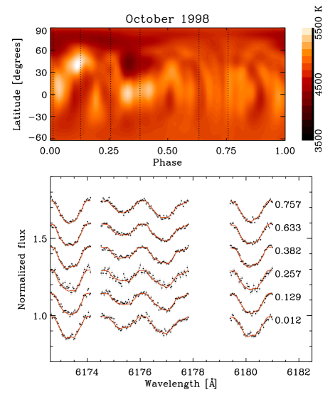
Figure 1: Top Temperature maps in equirectangular projection. The phase is defined in Eq. 1, and phases of observations are marked by vertical dashed lines. Bottom Normalized flux of the spectral region used for the inversion. Points are observations with error, the solid red line is the model calculated from the DI solution. The phase of each observation is listed to the right of the lines.

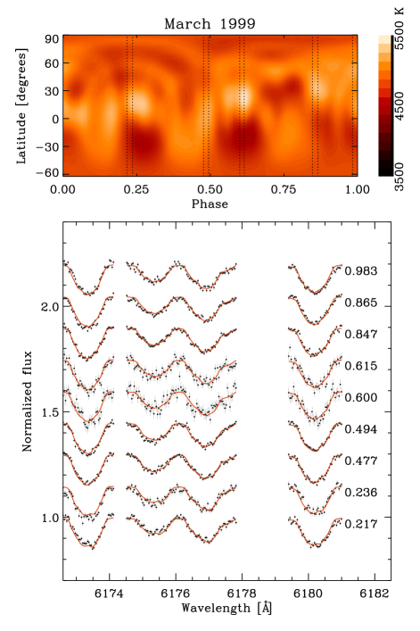
Figure 2: Same as in Figure 1 for the March 1999 observing season.

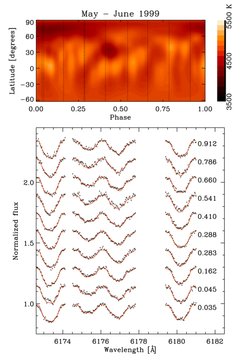
Figure 3: Same as in Figure 1 for the May - June 1999 observing season.

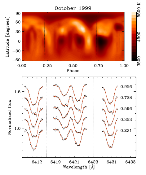
Figure 4: Same as in Figure 1 for the October 1999 observing season. A different spectral region was used due to different instrument setup.

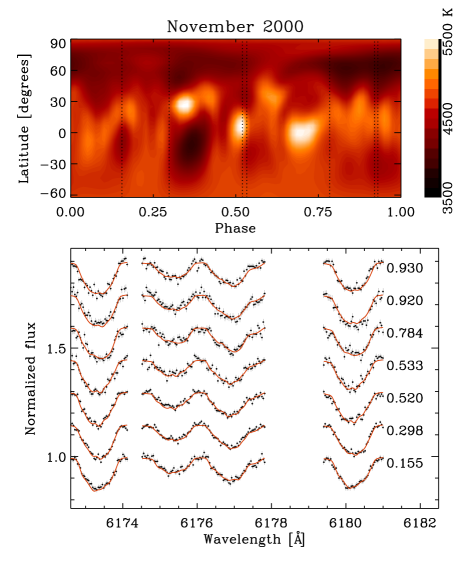
Figure 5: Same as in Figure 1 for the November 2000 observing season.

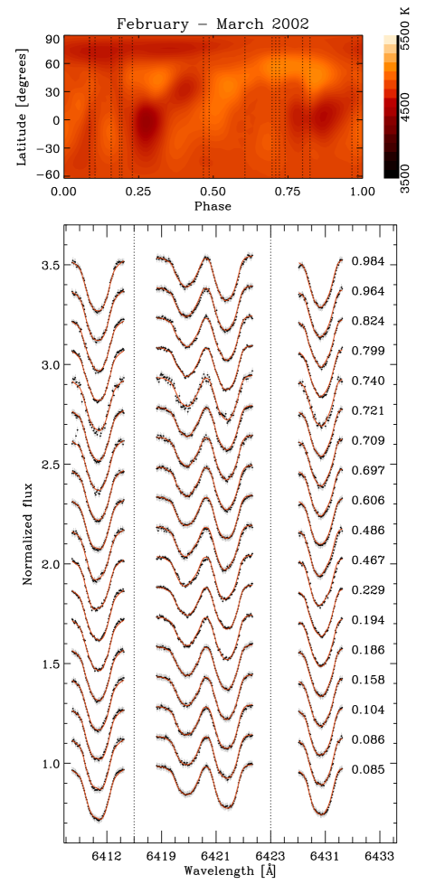
Figure 6: Same as in Figure 1 for the February-March 2002 observing seasons. This is the same spectral region as in Figure 4

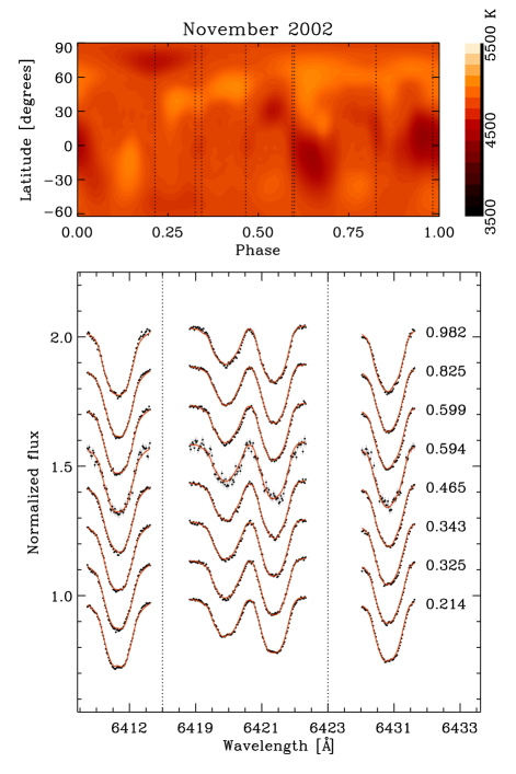
Figure 7: Same as in Figure 1 for the November 2002 observing seasons. This is the same spectral region as in Figure 4

The inversions are sensitive to phase coverage and S/N. Lower values in either of these for an observing season introduce artifacts in the temperature maps. Certain quantities are more meaningful in these cases than others. Phases of spots can be confirmed by examining the spectral lines corresponding to each map. Bumps similarly visible in multiple spectral lines are possible evidence for the presence of a real spot. The mean temperature $\langle T\rangle$ is calculated over the visible surface of the star and as such, any effects from noise or low phase coverage should cancel out with the appearance of both cooler and hotter regions.

However, spot temperature is sensitive to phase coverage and noise. Hot regions in the temperature maps may be physical, but are also possibly artifacts related either to noise or poor phase coverage. Latitude should also be taken with a grain of salt, particularly with spots below the equator. The lower the phase coverage, the less information available for the inversion program to distinguish latitudes of spots as being above or below the equator. The inversion method may also interpret sudden changes in spots during the observing season as spots at lower latitudes. A spot at a low latitude would only appear during a limited phase range, and sudden spot changes at higher latitudes would have similarly limited phase ranges. For spots close to the equator, noise or errors from the continuum level can create artifacts. Arches and ovals that appear in the temperature maps are also artifacts, usually related to noise or poor phase coverage. Due to the limitations imposed by the inversion method and the resolution of the maps, it is not possible to determine if a spot is a single feature or a composite of multiple spots located near each other.

The Oct98 map (Fig. 1) shows clear artifacts, mainly arches and hot spots in the temperature maps. Due to the low phase coverage and S/N, the latitude of spots and spot temperatures should be viewed with some skepticism. Mar99 (Fig. 2) has slightly poorer phase coverage, artifacts, and little evidence for spots within the observed phases, as those that appear to coincide with poorer S/N. May99 (Fig. 3) has decent phase coverage and S/N, with evenly spaced observations, and minimal appearance of ovals, arches, or hot and cool spot pairings. Oct99 (Fig. 4) has poor phase coverage but S/N is improved. Spots at certain phases are distinctly visible in the spectral line profiles as consistent deep bumps in multiple lines. So while information regarding latitude and spot shape cannot be inferred from this map, the phase of spots is likely physical and the amplitude of the bump supports a large temperature different between the spot and $\langle T\rangle$. Nov00 (Fig. 5) has a lower S/N and poorer phase coverage and shows similar evidence of artifacts as Oct99. However, spot phase and mean temperature are still meaningful due to the proximity of spots to the observed phases, but unlike the previous season, the noisier spectra make it difficult to determine if the spot temperature is due to artifacts or physical. Feb02 (Fig. 6) has the best phase coverage of all the observing seasons, and Nov02 (Fig. 7) has the highest S/N. These two are therefore the most reliable maps.

5 Discussion

Figure 8: Magnitudes are taken from Lehtinen et al. (2012a). Mean temperature, temperature difference, and spot coverage. Symbol sizes are proportional to the S/N-ratio and phase coverage so that a larger symbol indicates more reliable results.

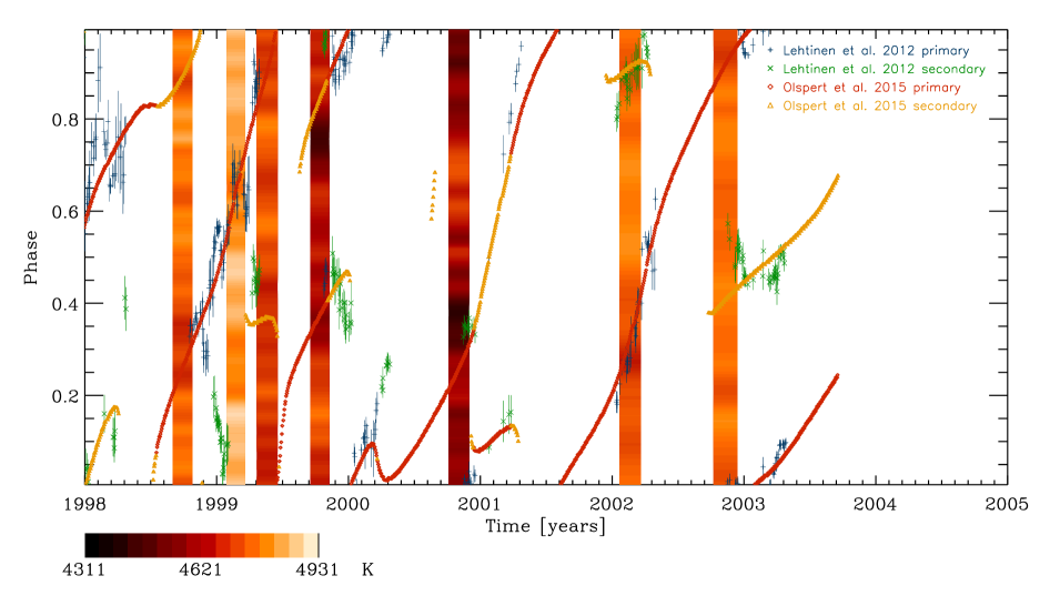
Figure 9: Longitudinal spot distribution from October 1998 to November 2002. Temperature is averaged over all latitudes for the Doppler Images. Also plotted are the photometric minimum epochs with error bars from Lehtinen et al. (2012a). Minimum epochs were obtained using the CPS method. For a more in-depth explanation, see Lehtinen et al. (2012b). Minima epochs from Olspert et al. (2014) were obtained using the CF method.

Table 4: Spot Coverage, mean temperature, and spot temperature difference from the mean.

Season	$n_{\phi}$	Spot Coverage	$\langle T\rangle$	$\Delta T$
Oct98	60%	6.0%	4790	350
Mar99	57%	2.3%	4850	430
May99	72%	5.8%	4730	360
Oct99	50%	22.7%	4630	590
Nov00	57%	32.2%	4600	810
Feb02	80%	1.9%	4740	420
Nov02	62%	4.5%	4740	310

Table 5: Observing season February-March 2002 with original and reduced phase coverage obtained by selecting 5 out of 18 observations.

$f_{\phi}$	Spot Coverage	$\langle T\rangle$	$\Delta T$
80%	1.9%	4740	420
50%	9.3%	4710	700

For the spot coverage analysis, all surface elements having $T_{\rm eff}\leq 4500$K were regarded as spots. Table 4 contains the mean temperature, coolest spot temperature, and spot coverage for each season. Figure 8 illustrates these values in relation to the photometry. Results that are less certain due to either low S/N or phase coverage are represented by smaller symbols. We tested the robustness of the inversion against phase gaps by taking the observing season with the best phase coverage, February-March 2002, and use only 5 observations from the 18 available. Table 5 is the comparison of these two maps. While $\langle T\rangle$ is pretty consistent, reducing the phase coverage increased the spot filling factor from 1.9% to 9.3% and decreased the minimum temperature of the map. Therefore, we can conclude that the spot filling factor may be overestimated by a similar factor in the low phase coverage maps.

Spot coverage is low for most seasons, but increases for seasons October 1999 and November 2000. These seasons coincide with an observed decrease in photometric magnitude (Lehtinen et al. 2012b). Even accounting for a low phase coverage, the spot filling factor is still highest during this point with a corresponding decrease in $\langle T\rangle$. We could consider this evidence of a possible cycle, with a high activity state during October 1999 - November 2000. In the work of Jetsu (1993), a cycle of 6.24 years was obtained from time series analysis. The ephemeris for the minimum of the mean brightness was calculated to be $(1981.^{\rm{y}}49\pm 0.^{\rm{y}}12)+(6.^{\rm{y}}24\pm 0.^{\rm{y}}26)$E. This would place the mean minimum brightness, or the highest spot activity, at $2000.^{\rm{y}}21$, or about March, 2000, which is in agreement with the higher spot coverage found during the months preceeding this ephemeris, even when accounting for low phase coverage.

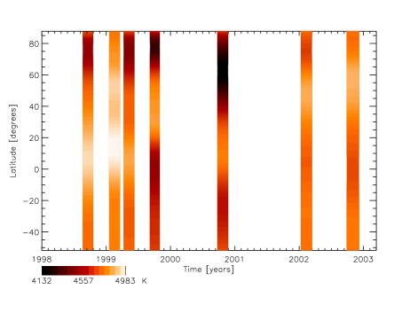
Figure 10: Latitudinal spot distribution from October 1998 to November 2002. Temperature is averaged over all longitudes for the Doppler Images.

Figure 9 shows the longitudinal spot distributions by averaging over the latitudinal direction. This mimics the results one could obtain from photometric observations, where only phase and magnitude of the star at a particular point of time is observed. We have marked the primary and secondary minimum epochs retrieved from light curves from both Lehtinen et al. (2012a) and from Olspert et al. (2014) using the Contiuous Period Search (hereafter CPS) and Carrier Fit (hereafter CF) methods respectively. Many seasons show good agreement with the photometry. For instance, in February-March 2002 both the results from Lehtinen et al. (2012b) and Olspert et al. (2014) agree with each other and match the recovered phases of spot locations in the Doppler images. The photometric studies coinciding with our DI seasons reveal an especially chaotic spot activity with non-persistent phase jumps. No coherent active longitudes are seen during this epoch. The period used to phase our observations in longitude is not optimally describing the rotation of the spot structures, evidenced by the upward trend in the global CF fit results. This is indicative of spot structures moving more slowly than the accepted rotation period of the star. The trend is disrupted at several points, and it would appear that the $P_{\rm rot}$ from Jetsu (1993) is not coherent for the length of time of this study. Olspert et al. (2014) find occurrences of flip-flop type events (sudden switches in the phase of the primary and secondary minima) coinciding with our observing seasons of October 1999 and November 2000. We find no evidence of active longitudes (phases with persistent spots over multiple observing seasons), and our spot phases are not in agreement with the ones listed in Berdyugina et al. (2002), and any similar conversion of spot phases into primary and secondary minima reveals no tendency for these spot structures to be consistently spaced approximately $180\degr$ apart.

We compare our maps to previous DI results. We average the temperature distribution over longitude in Fig. 10 to facilitate this, keeping in mind that the spot latitude is less reliable for October 1998, October 1999, and November 2000. There is a somewhat bimodal distribution with a dark band at or near the equator for most seasons as well as a second dark band near the pole. This is exaggerated for observing seasons with poorer phase coverage.

Early DI results by Strassmeier et al. (1993) for January and February 1991 show spots at mid-latitudes and polar features when using specific single spectral lines. However, temperature maps from observations during March, 1995 by Rice & Strassmeier (1998) have a band of spots centered around the equator and a slight polar feature. The reliable maps of this study show similar weak high-latitude spots, but no bands.

Our observations coincide approximately with DI by Kovári et al. (2004) and the ZDI by Donati et al. (2003b), time-wise. Kovári et al. (2004) observe an increase in spot coverage from November and December 1996 to April and May 2000. Our temperature maps show a similar increase in the spot coverage around October 1999. In contrast to the April and May 2000 maps, our October 1999 and November 2000 maps have no band of spots, although there are several cool spots located near the equator, but the latitude is not reliable in these two maps.

Donati (1999) and Donati et al. (2003b) published ZDI maps spanning over 10 years. The spot occupancy results, roughly comparable to temperature maps, are sensitive to phase coverage of an observing season. Because of this, more reliable seasons have higher spot occupancy and so it is difficult to make a comparison between spot occupancy maps and our temperature maps with regards to an activity cycle. The bimodal distribution of spots near the pole and near the equator is in agreement with our results.

Fekel et al. (1986b) proposed that spot evolution for single variable stars would occur more consistently and change slower for variable stars in binary systems. Henry et al. (1995) disagreed, postulating that the Roche lobe would have a stabilizing influence and result in a more consistent spot evolution. Recent results and this report support the latter conclusion. Studies of RS CVn type stars in binary systems such as II Peg and $σ$ Gem seem to display more stable behaviour (Hackman et al. 2012; Kajatkari et al. 2014) whereas single type stars such as HD 116956 and FK Com displayed more chaotic behaviour (Lehtinen et al. 2011; Hackman et al. 2013). LQ  Hya fits in this latter group, and the DI results support this. There is no appearance of long-lived structures even within the 4-year time span of maps in this report, and while a possible cycle is evident, the spot structure evolution over time gives no indication of stability.

6 Conclusions

We have a total of 7 observing seasons from 1998-2002. There is a possible cycle with a rise and subsequent fall in stellar activity, using the spot coverage and mean temperature as an indication of activity (Fig. 8). This cycle approximately matches a predicted cycle from Jetsu (1993), where a decrease in brightness corresponds to an increase in spot coverage and therefore activity level.

We compare the Doppler images to photometry. LQ Hya does not have a consistent spot structure over a long period of time, unlike other studied objects such as II Peg.

There is some evidence for a high-latitude spot, but it is not persistent and mainly appears during the higher activity seasons. There is no evidence of active longitudes over multiple observing seasons, and this is consistent with recent findings using photometry (Lehtinen et al. 2012b; Olspert et al. 2014). Spots possibly have a bimodal distribution (Fig. 10). and the spot coverage (areas with temperatures $\leq 4500$K), ranges from covering a small amount to a third of the star. The cycle length cannot be inferred from only 4 years of observations. An activity minimum coincides with a 6.24 postulated activity cycle, but the baseline of observations falls short of a full cycle length of 6-7 years. The spot activity is chaotic with flip-flop events in photometry occurring during maximum spot coverage.

Table 6: All Observations. S/N is calculated is taken from observation data within the wavelength regions used in the analysis. HJD is -2 450 000.

Date	HJD	$\phi$	S/N	Date	HJD	$\phi$	S/N	Date	HJD	$\phi$	S/N
(dd/mm/yyyy)	-2450000			(dd/mm/yyyy)	-2450000			(dd/mm/yyyy)	-2450000
03/10/1998	1089.7527	0.129	96	31/05/1999	1330.3727	0.410	127	24/02/2002	2329.6036	0.486	162
04/10/1998	1090.7580	0.757	100	01/06/1999	1331.3730	0.035	116	25/02/2002	2330.5620	0.085	279
05/10/1998	1091.7580	0.382	116	02/06/1999	1332.3736	0.660	128	26/02/2002	2331.5424	0.697	212
06/10/1998	1092.7668	0.012	79	03/06/1999	1333.3713	0.283	120	26/02/2002	2331.5807	0.721	194
07/10/1998	1093.7616	0.633	107	20/10/1999	1471.7823	0.728	91	28/02/2002	2333.5716	0.964	166
08/10/1998	1094.7614	0.257	60	21/10/1999	1472.7819	0.353	127	28/02/2002	2333.6028	0.984	184
02/03/1999	1240.3999	0.217	99	22/10/1999	1473.7487	0.956	179	01/03/2002	2334.5984	0.606	283
02/03/1999	1240.4303	0.236	81	23/10/1999	1474.7724	0.596	121	01/03/2002	2335.4832	0.158	196
03/03/1999	1241.4083	0.847	120	24/10/1999	1475.7729	0.221	107	02/03/2002	2335.5272	0.186	272
03/03/1999	1241.4370	0.865	131	06/11/2000	1854.7606	0.920	63	05/03/2002	2338.5694	0.086	169
04/03/1999	1241.6267	0.983	101	07/11/2000	1855.7428	0.533	80	05/03/2002	2338.5981	0.104	190
04/03/1999	1242.4180	0.477	123	08/11/2000	1856.7381	0.155	85	06/03/2002	2339.5679	0.709	127
04/03/1999	1242.4450	0.494	132	09/11/2000	1857.7453	0.784	69	06/03/2002	2339.6174	0.740	70
05/03/1999	1242.6140	0.600	43	13/11/2000	1861.7711	0.298	125	10/11/2002	2588.7586	0.343	263
05/03/1999	1242.6387	0.615	54	14/11/2000	1862.7830	0.930	83	12/11/2002	2590.7615	0.594	72
24/05/1999	1323.3832	0.045	97	15/11/2000	1863.7269	0.520	104	18/11/2002	2596.7350	0.325	233
26/05/1999	1325.3739	0.288	145	22/02/2002	2327.5345	0.194	165	21/11/2002	2599.7598	0.214	331
27/05/1999	1326.3735	0.912	100	22/02/2002	2327.5901	0.229	245	22/11/2002	2600.7389	0.825	353
28/05/1999	1327.3805	0.541	78	22/02/2002	2328.5040	0.799	201	23/11/2002	2601.7633	0.465	235
29/05/1999	1328.3741	0.162	124	23/02/2002	2328.5435	0.824	162	27/11/2002	2605.7937	0.982	205
30/05/1999	1329.3732	0.786	91	24/02/2002	2329.5725	0.467	156	28/11/2002	2606.7807	0.599	231