Reconstruction within the Zeldovich approximation

Abstract

The Zeldovich approximation, $1^{\rm st}$ order Lagrangian perturbation theory, provides a good description of the clustering of matter and galaxies on large scales. The acoustic feature in the large-scale correlation function of galaxies imprinted by sound waves in the early Universe has been successfully used as a ‘standard ruler’ to constrain the expansion history of the Universe. The standard ruler can be improved if a process known as density field reconstruction is employed. In this paper we develop the Zeldovich formalism to compute the correlation function of biased tracers in both real- and redshift-space using the simplest reconstruction algorithm with a Gaussian kernel and compare to N-body simulations. The model qualitatively describes the effects of reconstruction on the simulations, though its quantitative success depends upon how redshift-space distortions are handled in the reconstruction algorithm.

1 Introduction

The large-scale structure seen in the distribution of galaxies contains a wealth of information about the nature and constituents of our Universe. Of particular interest here is the use of low-order statistics of this field to constrain the distance scale and growth rate of fluctuations, which in turn impact upon our understanding of dark energy and tests of General Relativity at cosmological scales (e.g. Olive et al., 2014). One of the premier methods for measuring the distance scale uses the baryon acoustic oscillation (BAO) ‘feature’ in the 2-point function of galaxies as a calibrated, standard ruler (see Olive et al., 2014, for a review). Additional information on the rate of growth of perturbations, which allows a key test of General Relativity and constraints on modified gravity (e.g. Joyce et al., 2014, and references therein), is encoded in the anisotropy of the 2-point function imprinted by peculiar velocities, i.e. redshift space distortions (see Hamilton, 1998, for a review). Fits to the distance scale using the BAO feature become significantly more accurate if density field ‘reconstruction’ is applied (Eisenstein, et al., 2007a), but this procedure alters the signal that is used to infer the growth rate from redshift-space distortions. Ideally we would have a model which can simultaneously describe the features which are used to constrain distance scale and the growth of structure, since there is a non-trivial degeneracy between mis-estimates of distance and growth (e.g. Fig. 9 of Reid et al., 2012). A formalism which can be used to simultaneously describe both of these pieces of a redshift survey is currently not known.

It is straightforward to form a data vector which consists of the correlation function pre-reconstruction on small scales and post-reconstruction on large scales. Our goal is to find a single theoretical framework which could simultaneously fit both parts of this data vector. Models based upon Lagrangian perturbation theory have been shown to do a good job of fitting the anisotropic signal in the (pre-reconstruction) correlation function (see e.g. White et al. 2015 for a recent investigation and references to the earlier literature). In this paper we investigate how accurately $1^{\rm st}$ order Lagrangian perturbation theory (“the Zeldovich approximation”) can be used to model the reconstructed BAO feature in the redshift-space correlation function of biased tracers.

The last few years have seen a resurgence of interest in the Zeldovich approximation. It has been applied to understanding the effects of non-linear structure formation on the baryon acoustic oscillation feature in the correlation function (Padmanabhan & White, 2009; McCullagh & Szalay, 2012; Tassev & Zaldarriaga, 2012a) and to understanding how “reconstruction” (Eisenstein, et al., 2007a) removes those non-linearities (Padmanabhan, White & Cohn, 2009; Noh, White & Padmanabhan, 2009; Tassev & Zaldarriaga, 2012b). It has been used as the basis for an effective field theory of large-scale structure (Porto, Senatore & Zaldarriaga, 2014) and a new version of the halo model (Seljak & Vlah, 2015). It has been compared to “standard” perturbation theory (Tassev, 2014a), extended to higher orders in Lagrangian perturbation theory (Matsubara, 2008a, b; Okamura, Taruya, & Matsubara, 2011; Carlson, Reid & White, 2013; Vlah, Seljak & Baldauf, 2015) and to higher order statistics (Tassev, 2014b) including a model for the power spectrum covariance matrix (Mohammed & Seljak, 2014). Despite the more than 40 years since it was introduced, the Zeldovich approximation still provides one of our most accurate models for the distribution of cosmological objects.

The outline of the paper is as follows. Section 2 contains a review of the salient aspects of Lagrangian perturbation theory and reconstruction, to fix our notation, and introduces our N-body simulations. Section 3 introduces the Zeldovich model for reconstruction and compares its predictions to the simulations. We finish in Section 4 with an assessment of the Zeldovich approximation and future directions for research.

2 Background and review

2.1 Lagrangian perturbation theory

We wish to develop an analytic description of the reconstructed correlation function of biased tracers in redshift space and to this end we use Lagrangian perturbation theory (Buchert, 1989; Moutarde et al., 1991; Hivon et al., 1995; Taylor & Hamilton, 1996). In this section we remind the reader of some essential terminology, and establish our notational conventions. Our notation and formalism follows closely that in Matsubara (2008a, b); Carlson, Reid & White (2013); Wang, Reid & White (2013); White (2014) to which we refer the reader for further details and original references.

In the Lagrangian approach to cosmological fluid dynamics, one traces the trajectory of an individual fluid element through space and time. Every element of the fluid is uniquely labeled by its Lagrangian coordinate $\mathbf{q}$ and the displacement field $\mathbf{\Psi}(\mathbf{q},t)$ fully specifies the motion of the cosmological fluid. Lagrangian Perturbation Theory (LPT) develops a perturbative solution for $\mathbf{\Psi}$ but we shall deal here with the first order solution which is known as the Zeldovich approximation (Zeldovich, 1970). Denote this first order solution as $\mathbf{\Psi}$ we have:

$$\mathbf{\Psi}(\mathbf{q})=\int\frac{d^{3}k}{(2\pi)^{3}}\ e^{i\mathbf{k}\cdot\mathbf{q}}\frac{i\mathbf{k}}{k^{2}}\delta_{L}(\mathbf{k}),$$ (1)

We shall assume that halos, and the galaxies that inhabit them, have a local Lagrangian bias $\rho_{X}(\mathbf{q})=\bar{\rho}_{X}F[\delta_{R}(\mathbf{q})]$. Matsubara (2011) provides an extensive discussion of local and non-local Lagrangian bias schemes.

This formalism makes it particularly easy to include redshift space distortions. We follow the earlier papers and adopt the “plane-parallel” or “distant-observer” approximation, in which the line-of-sight direction to each object is taken to be the fixed direction $\hat{z}$. Within this approximation, including redshift-space distortions is achieved via

$$\Psi_{i}\to\Psi_{i}^{s}=R_{ij}\Psi_{j}=(\delta_{ij}+f\hat{z}_{i}\hat{z}_{j})\Psi_{j}$$ (2)

which simply multiplies the $z$-component of the vector by $1+f$.

The correlation function within the Zeldovich approximation then follows by elementary manipulations. Defining $\Delta\equiv\mathbf{\Psi}_{2}-\mathbf{\Psi}_{1}$ and writing $F_{i}=F(\lambda_{i})$ for the Fourier transform of $F[\delta_{R}(\mathbf{q})]$ the real-space correlation function is

$$1+\xi_{X}(\mathbf{r}) = \int d^{3}q\int\frac{d^{3}k}{(2\pi)^{3}}e^{i\mathbf{k}\cdot(\mathbf{q}-\mathbf{r})}\int\frac{d\lambda_{1}}{2\pi}\frac{d\lambda_{2}}{2\pi}\ F_{1}F_{2}$$ (3)

$$\times \left\langle e^{i(\lambda_{1}\delta_{1}+\lambda_{2}\delta_{2}+\mathbf{k}\cdot\mathbf{\Delta})}\right\rangle.$$

For convenience we define $\xi_{L}(\mathbf{q})=\langle\delta_{1}\delta_{2}\rangle$, $U_{i}(\mathbf{q})=\langle\delta_{1}\Delta_{i}\rangle=\langle\delta_{2}\Delta_{i}\rangle$, and $A_{ij}(\mathbf{q})=\langle\Delta_{i}\Delta_{j}\rangle$. The vector $U_{i}(\mathbf{q})=U(q)\,\hat{q}_{i}$ is the cross-correlation between the linear density field and the Lagrangian displacement field. The matrix $A_{ij}$ may be decomposed as

$$A_{ij}(\mathbf{q}) = 2\left[\sigma_{\eta}^{2}-\eta_{\perp}(q)\right]\delta_{ij}+2\left[\eta_{\perp}(q)-\eta_{\parallel}(q)\right]\hat{q}_{i}\hat{q}_{j},$$ (4)

$$= \sigma_{\perp}^{2}\delta_{ij}+\left[\sigma_{\parallel}^{2}-\sigma_{\perp}^{2}\right]\hat{q}_{i}\hat{q}_{j}$$ (5)

where $\sigma_{\eta}^{2}\equiv\frac{1}{3}\langle|\mathbf{\Psi}|^{2}\rangle$ is the 1-D dispersion of the displacement field, and $\eta_{\parallel}$ and $\eta_{\perp}$ are the transverse and longitudinal components of the Lagrangian 2-point function, $\eta_{ij}(\mathbf{q})=\left\langle\Psi_{i}(\mathbf{q}_{1})\Psi_{j}(\mathbf{q}_{2})\right\rangle$. In the Zeldovich approximation these quantities are given by simple integrals over the linear power spectrum:

$$\sigma_{\eta}^{2}=\frac{1}{6\pi^{2}}\int_{0}^{\infty}dk~{}P_{L}(k),$$ (6)

$$\eta_{\perp}(q)=\frac{1}{2\pi^{2}}\int_{0}^{\infty}dk~{}P_{L}(k)~{}\frac{j_{1}(kq)}{kq},$$ (7)

$$\eta_{\parallel}(q)=\frac{1}{2\pi^{2}}\int_{0}^{\infty}dk~{}P_{L}(k)~{}\left[j_{0}(kq)-2\frac{j_{1}(kq)}{kq}\right],$$ (8)

$$U(q)=-\frac{1}{2\pi^{2}}\int_{0}^{\infty}dk~{}kP_{L}(k)~{}j_{1}(kq).$$ (9)

Taylor series expanding the bias terms and doing the $\lambda_{1}$ and $\lambda_{2}$ integrations and the Fourier transform we can write

$$1+\xi_{X}(\mathbf{r}) = \int\frac{d^{3}q}{(2\pi)^{3/2}|A|^{1/2}}\ e^{-\frac{1}{2}(\mathbf{r}-\mathbf{q})^{T}\mathbf{A}^{-1}(\mathbf{r}-\mathbf{q})}\left[1+b_{1}^{2}\xi_{L}\right.$$ (10)

$$- 2b_{1}U_{i}g_{i}+\frac{1}{2}b_{2}^{2}\xi_{L}^{2}-(b_{2}+b_{1}^{2})U_{i}U_{j}G_{ij}$$

$$- \left.2b_{1}b_{2}\xi_{L}U_{i}g_{i}+\cdots\right],$$

where we have written $b_{n}=\left\langle F^{(n)}\right\rangle$, $g_{i}\equiv(A^{-1})_{ij}(q-r)_{j}$ and $G_{ij}\equiv(A^{-1})_{ij}-g_{i}g_{j}$ in order to make the expressions more readable. The generalization to redshift space follows straightforwardly from Eq. (2): we simply multiply $U_{z}$ by $1+f$ and divide the $z$-components of $\mathbf{A}^{-1}$ by the same factor.

Not all of the terms in Eq. (10) are important at the scales relevant for BAO. For typical values of halo bias ($b_{1}\sim 1$ and $b_{2}\sim 0.1$), the dominant contributions to the real space correlation function or the monopole of the redshift space correlation function at $r\simeq 100\,h^{-1}$Mpc are from the “1”, $b_{1}^{2}\xi_{L}$ and $-2b_{1}U_{i}g_{i}$ terms. The other terms make up less than one per cent of the total. For the quadrupole of the redshift space correlation function only the the “1” and $-2b_{1}U_{i}g_{i}$ terms contribute significantly (see also White, 2014, Fig. 4).

2.2 Reconstruction

We start by reviewing the reconstruction algorithm of Eisenstein, et al. (2007a) and its interpretation within Lagrangian perturbation theory (Padmanabhan, White & Cohn, 2009; Noh, White & Padmanabhan, 2009). Various tests of reconstruction have been performed in Seo et al. (2010); Padmanabhan et al. (2012); Xu et al. (2013); Burden et al. (2014); Tojiero et al. (2014) which also contain useful details on the specific implementations.

The algorithm devised by Eisenstein, et al. (2007a) is straightforward to apply and consists of the following steps:

• Smooth the halo or galaxy density field with a kernel $\mathcal{S}$ (see below) to filter out small scale (high $k$) modes, which are difficult to model. Divide the amplitude of the overdensity by an estimate of the large-scale bias, $b$, to obtain a proxy for the overdensity field: $\delta(\mathbf{x})$.

• Compute the shift, $\mathbf{s}$, from the smoothed density field in redshift space using the Zeldovich approximation (this field obeys $\mathbf{\nabla}\cdot\mathbf{R}\mathbf{s}=-\delta$ with the $f$ replaced by $f/b$ in $\mathbf{R}$). The line-of-sight component of $\mathbf{s}$ is multiplied by $1+f$ to approximately account for redshift-space distortions.

• Move the galaxies by $\mathbf{s}$ and compute the “displaced” density field, $\delta_{d}$.

• Shift an initially spatially uniform distribution of particles by $\mathbf{s}$ to form the “shifted” density field, $\delta_{s}$. It is ambiguous whether this shift includes the factor of $1+f$ in the line-of-sight direction or not. Including the $1+f$ includes ‘linear’ redshift-space distortions in the reconstructed field while excluding it removed them. Padmanabhan et al. (2012); Xu et al. (2013) and later works do not include this factor, but earlier papers did not distinguish between the uniform sample and the galaxies. We shall consider both approaches.

• The reconstructed density field is defined as $\delta_{r}\equiv\delta_{d}-\delta_{s}$ with power spectrum $P_{r}(k)\propto\langle\left|\delta_{r}^{2}\right|\rangle$.

Following Eisenstein, et al. (2007a) we use a Gaussian smoothing of scale $R$, specifically $\mathcal{S}(k)=e^{-(kR)^{2}/2}$. Throughout we shall assume that the fiducial cosmology, bias and $f$ are properly known during reconstruction. Padmanabhan et al. (2012); Xu et al. (2013); Burden et al. (2014); Vargas-Magana et al. (2014) show that the reconstructed 2-point function is quite insensitive to the specific choices made, so this is a reasonable first approximation. We shall return to this issue in Section 4.

2.3 N-body simulations

We use a suite of 20 N-body simulations to test how well the Zeldovich model works. The simulations assume a $\Lambda$CDM cosmology with $\Omega_{m}=0.274$, $\Omega_{\Lambda}=0.726$, $h=0.7$, $n=0.95$, and $\sigma_{8}=0.8$ and were run with the TreePM code described in White (2002). Each simulation employed $1500^{3}$ equal mass ($m_{p}\simeq 7.6\times 10^{10}\,h^{-1}M_{\odot}$) particles in a periodic cube of side length $1.5\,h^{-1}$Gpc as described in Reid & White (2011) and White et al. (2011). Halos are found using the friends-of-friends method, with a linking length of $0.168$ times the mean inter-particle spacing. These are the same simulations and catalogs that were used in Wang, Reid & White (2013); White (2014); White et al. (2015) and further details can be found in those papers. Throughout we shall use halos with friends-of-friends mass in the range $12.785<\log_{10}M_{h}/(h^{-1}M_{\odot})<13.085$, with $b\simeq 1.7$, which is one of the samples used in Wang, Reid & White (2013); White (2014). It has a relatively high bias, while at the same time a large enough spatial density to reduce shot noise to tolerable levels.

3 Zeldovich reconstructed

With this background in hand it is now straightforward to develop a model for the reconstructed correlation function within the Zeldovich approximation.

3.1 The shift

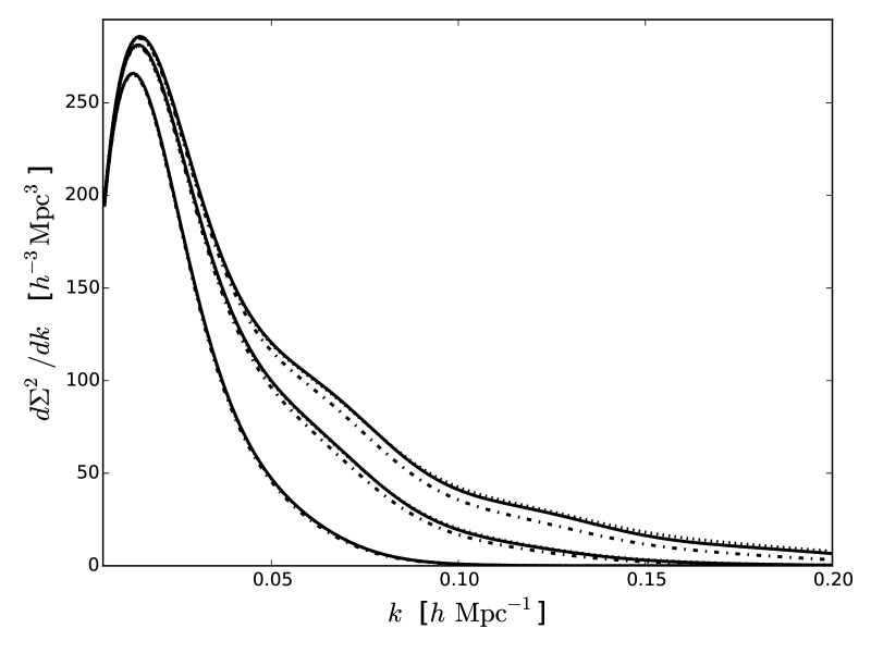
Figure 1: The contribution to the variance of the 1D Zeldovich displacement, per unit $k$, at $z\simeq 0.5$ for three different (Gaussian) smoothing scales: $R=5$, 10 and $20\,h^{-1}$Mpc (upper to lower sets of lines). For each set of lines the solid line is the linear theory prediction, the dashed line assumes standard, $2^{\rm nd}$ order, Eulerian perturbation theory and the dot-dashed line is the Zeldovich approximation expanded to $2^{\rm nd}$ order. Except for the $5\,h^{-1}$Mpc case all three approximations are in excellent agreement (see also Fig. 1 of Padmanabhan, White & Cohn 2009).

We will assume that the “shift” field, which is formally computed on the non-linear density field at the Eulerian position, $\mathbf{x}$, can be well approximated by the negative Zeldovich displacement computed from the linear theory field at the Lagrangian position, $\mathbf{q}$. This is a reasonable first approximation since such shifts are dominated by very long wavelength modes (Eisenstein, et al., 2007b). The difference between $\delta_{L}(\mathbf{q})$ and $\delta_{L}(\mathbf{x})$ is higher-order in $\mathbf{\Psi}$ and so should be comparable to the effect of non-linearities in the density. Within the same approximation, solving $\mathbf{\nabla}\cdot\mathbf{R}\mathbf{s}=-\delta$ on the redshift-space field is the same as generating $\mathbf{s}(\mathbf{k})=-i(\mathbf{k}/k^{2})\delta(\mathbf{k})\mathcal{S}(k)$ using the real-space field.

To estimate the relative size of the correction to the shift terms coming from non-linearities in the density, we look at the contributions to the rms Zeldovich displacement for different (Gaussian) smoothing scales, $R$. In real space the 1D displacement is $\left[\int dk\,P(k)/(6\pi^{2})\right]^{1/2}$. Fig. 1 shows the fractional contribution to the squared displacement from beyond-linear terms in $P(k)$, computed from (standard) Eulerian perturbation theory or the Zeldovich approximation [see Appendix A for more details]. For smoothings of $10\,h^{-1}$Mpc or above the approximation appears to be very good. We shall use $R=15\,h^{-1}$Mpc as our default (as used in e.g. Padmanabhan et al., 2012; Anderson et al., 2014; Tojiero et al., 2014), unless otherwise specified.

Under this approximation we compute the statistics of the displaced field by replacing $\mathbf{\Psi}$ with $\mathbf{\Psi}+\mathbf{s}$ and of the shifted field by replacing $\mathbf{\Psi}$ with $\mathbf{s}$ in the formulae of §2.

3.2 Real space

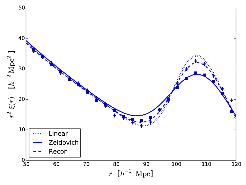
Figure 2: A comparison of the Zeldovich and N-body real-space, halo correlation functions pre- and post-reconstruction. The dotted line shows the linear theory, while the solid (dashed) line shows the Zeldovich prediction pre(post)-reconstruction. The squares and diamonds show the unreconstructed and reconstructed results from the N-body simulations described in the text. We have used a smoothing scale of $R=15\,h^{-1}$Mpc when performing reconstruction.

Let us first consider the statistics of the reconstructed field in real space. The reconstructed field is the sum of the displaced and the negative of the shifted fields of Sec. 2.2 and thus the correlation function has 3 terms: the auto-correlation of the displaced field, the auto-correlation of the negative-shifted field and the cross-correlation of the two fields: $\xi^{(\rm recon)}=\xi^{(dd)}+\xi^{(ss)}+2\xi^{(ds)}$. Each term will have the same functional form as Eq. (10). Let us take each in turn. The auto-correlation function of the displaced field, $\xi^{(dd)}$, is given by Eq. (10) with $P_{L}\to P_{L}(1-\mathcal{S})^{2}$ when evaluating $\eta_{\perp}$ and $\eta_{\parallel}$ and one power of $1-\mathcal{S}$ when computing $U$ (it is unchanged when computing $\xi_{L}$). Thus for example the $U_{i}$ entering the analog of Eq. (10) for $\xi^{(dd)}$ is given by

$$U^{(dd)}(q)=-\frac{1}{2\pi^{2}}\int_{0}^{\infty}dk\,k\ P_{L}(k)\left(1-\mathcal{S}\right)\ j_{1}(kq).$$ (11)

and similarly for the other terms. The auto-correlation function of the shifted field is similarly given by Eq. (10) with $b_{1}=b_{2}=0$ (i.e. the terms in square brackets in Eq. (10) become $1$) and $P_{L}\to P_{L}\mathcal{S}^{2}$ when evaluating $\eta_{\perp}$ and $\eta_{\parallel}$ which define $A_{ij}$. The cross term between the displaced and shifted fields has $P_{L}\to P_{L}\mathcal{S}(1-\mathcal{S})$ when evaluating $\eta_{\perp}$ and $\eta_{\parallel}$ and $P_{L}\to P_{L}\mathcal{S}$ when evaluating $U$ and the substitutions $b_{1}\to\frac{1}{2}b_{1}$, $b_{2}\to\frac{1}{2}b_{2}$, $b_{1}^{2}\to 0$, $b_{2}^{2}\to 0$ and $b_{1}b_{2}\to 0$ in Eq. (10), i.e.

$$1+\xi_{X}^{(ds)}(\mathbf{r}) = \int\frac{d^{3}q}{(2\pi)^{3/2}|A^{(ds)}|^{1/2}}\ e^{-\frac{1}{2}(\mathbf{r}-\mathbf{q})^{T}\mathbf{A}_{(ds)}^{-1}(\mathbf{r}-\mathbf{q})}\left[1\right.$$ (12)

$$\left.-b_{1}U_{i}^{(ds)}g_{i}^{(ds)}-\frac{1}{2}b_{2}U_{i}^{(ds)}U_{j}^{(ds)}G_{ij}^{(ds)}+\cdots\right]$$

A comparison of the correlation function predicted by the Zeldovich approximation with that measured in N-body simulations is shown in Fig. 2. The theory predicts that the acoustic peak (at $r\simeq 110\,h^{-1}$Mpc) is broadened by the effects of non-linear structure formation and that reconstruction acts to sharpen the peak. The agreement with the simulations both pre- and post-reconstruction is quite good, as expected from the earlier work of Noh, White & Padmanabhan (2009, although in that work $2^{\rm nd}$ order LPT was used). While we do not have the necessary volume of simulations to reliably measure the peak location at sub-percent precision, we argue in the Appendix that the model should accurately reflect the manner in which reconstruction reduces the small shift in the peak location engendered by mode-coupling (see similar discussion in Padmanabhan & White 2009). We have checked that the agreement between the model and the simulations is qualitatively similar for variations in the smoothing scale between $10$ to $20\,h^{-1}$Mpc.

3.3 Redshift space

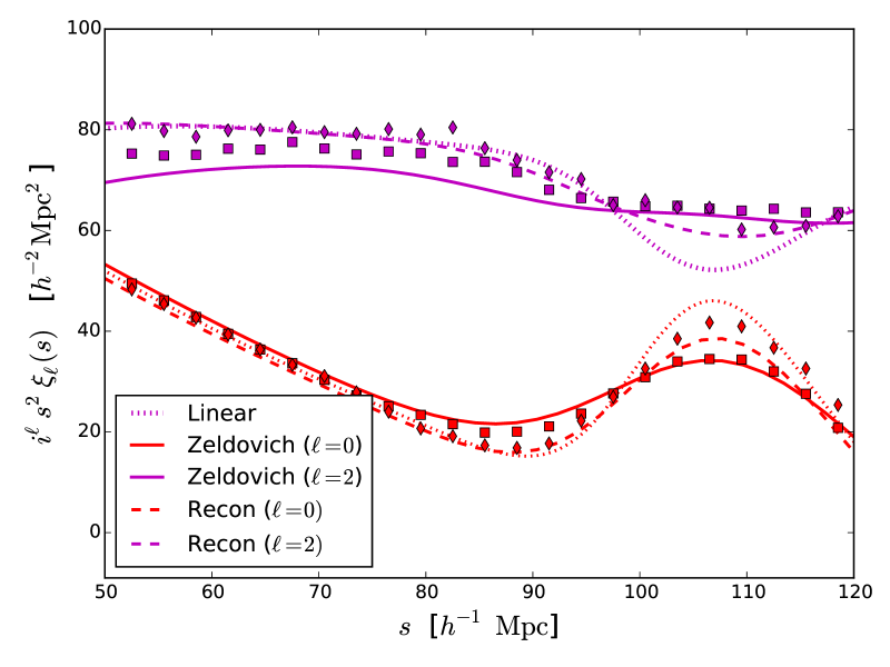
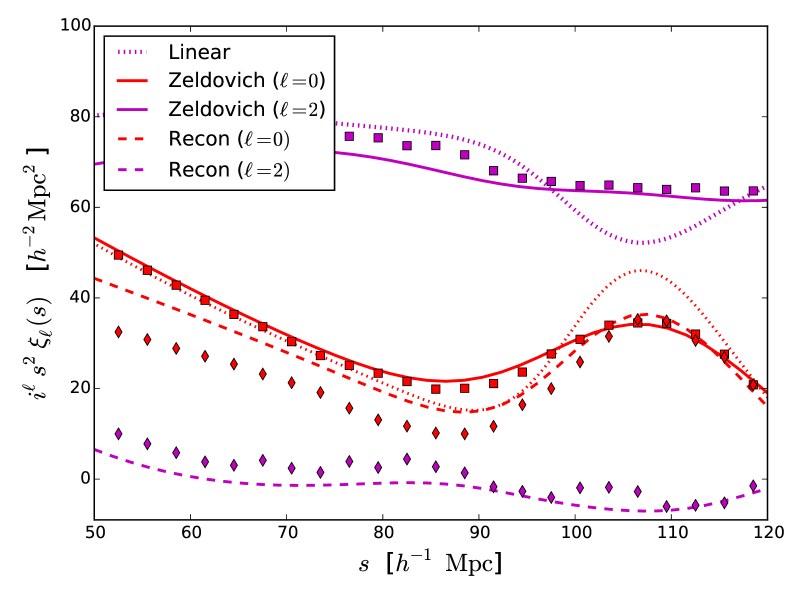
Figure 3: A comparison of the Zeldovich and N-body redshift-space, halo correlation functions pre- and post-reconstruction. The dotted line shows the linear theory, while the solid (dashed) line shows the Zeldovich prediction pre(post)-reconstruction. The squares and diamonds show the unreconstructed and reconstructed results from the N-body simulations described in the text. The upper set of lines are for the quadrupole while the lower set of lines is for the monopole except in the lower panel where the lowest dashed line is for the reconstructed quadrupole. Two versions of reconstruction are shown: (upper) with both the halos and the initially uniformly distributed particles shifted by the same field (lower) with the halos shifted $1+f$ times further in the line-of-sight direction than the uniform particles.

Now we turn to redshift space. If we use a single field, $\mathbf{s}$, to shift both the halos and the random particles (i.e. with the factor of $1+f$ in the line-of-sight direction for both) when generating $\mathbf{s}$ the modifications to the preceeding section are small: we simply multiply $U_{z}$ by $1+f$ and divide the $z$-components of $\mathbf{A}^{-1}$ by the same factor.

The upper panel of Fig. 3 shows the monopole and quadrupole of the correlation function in this case. The Zeldovich approximation does a credible job of fitting the monopole of the redshift-space, halo correlation function pre-reconstruction. The agreement for the quadrupole moment is better than linear theory in the acoustic peak region, but not as good as for the monopole (as expected from earlier work, e.g. White 2014, Fig. 2). To avoid cluttering the figure we have not plotted the errors on the N-body points. For the monopole they are generally small, but for the quadrupole (pre- and post-reconstruction) they are significant. In the acoustic peak region the typical error on $s^{2}\xi_{2}$ is $3-5\,h^{-2}{\rm Mpc}^{2}$ and the errors are highly correlated. Post-reconstruction the results for both multipoles of the correlation function are qualitatively similar: the reconstructed multipoles are closer to the linear theory than the evolved ones and the agreement with the N-body simulations in the region of the acoustic peak ($s\simeq 110\,h^{-1}$Mpc) is quite good. Unfortunately the errors on the quadrupole from the N-body simulations are too large to see whether the predicted shift from the pre- to post-reconstruction shape near the acoustic peak is borne out in simulations. If pushed to smaller scales the model starts to depart significantly from the simulation results, no doubt because the Zeldovich approximation does not accurately capture the anisotropies in the displacement/velocity field on smaller scales (see White, 2014, for further discussion). There is weak evidence that the Zeldovich approximation agrees better with the N-body simulations for the quadrupole moment after reconstruction than it does before. Increasing the smoothing scale (to $30\,h^{-1}$Mpc) leads to similar agreement between the simulation and model, but reduces the sharpening of the peak by reconstruction. Reducing the smoothing scale to $10\,h^{-1}$Mpc gives results very similar to those shown in Fig. 3.

An alternative formulation does not include the factor of $1+f$ in the line-of-sight shift for the initially uniformly distributed particles. This acts to reduce the effects of redshift-space distortions in the reconstructed density field. In this case the factors of $1+f$ are omitted entirely when computing the shift-shift auto-correlation function, and only one power of $1+f$ is included in $\mathbf{A}^{-1}$ and no factors of $1+f$ in $\mathbf{U}$ in the cross-correlation of the displaced and shifted particles but the rest of the terms remain unchanged. This is shown in the lower panel of Fig. 3 and the level of agreement between the theory and the simulations is similar to that in the upper panel. Note in the lower panel the quadrupole is significantly reduced in both the model and the simulations, indicating that we have removed most of the effects of linear redshift-space distortions, but it is not reduced entirely to zero (earlier investigations of reconstruction in simulations either did not include redshift-space distortions or presented only the monopole statistics). Again the numerical errors from the N-body simulation are not negligible, but the overall trends are clear. The agreement between the simulations and the model in the monopole is no longer as good on scales smaller than the acoustic peak as it was in the upper panel.

Comparing the upper and lower panels of Fig. 3 suggests that the errors in how the Zeldovich approximation models reconstruction partially cancel if both the galaxies and initially uniformly distributed sample of particles are shifted by the same field. In this case the agreement between the model and simulations in both the monopole and quadrupole moments of the correlation function above $90\,h^{-1}$Mpc is quite encouraging. If only the galaxies are shifted by an additional factor of $1+f$ in the line-of-sight direction the reduction in the quadrupole moment is qualitatively reproduced by the model but the well-known inaccuracies in the halo velocity field cause a significant over-estimate of the monopole even at $90\,h^{-1}$Mpc. If the Zeldovich approximation is to be used as a template for fitting the reconstructed BAO feature, it would be better to implement reconstruction on the data using the ‘both shift’ formalism. If the behavior of the model is improved because the ‘both shift’ formulation reduces sensitivity to small scales (where the model does less well) then this formulation may be less sensitive to small scales in the data as well and potentially more robust. Such an investigation is outside the scope of this work.

4 Discussion

The goal of this paper was to investigate a model for the reconstructed, redshift-space correlation function of biased tracers within the framework of Lagrangian perturbation theory. In principle such a model can be combined with other models within the same framework to fit a combination of data such as reconstructed BAO and redshift-space distortions, for example by fitting a data vector which consists of pre-reconstruction multipoles below $s\simeq 90\,h^{-1}$Mpc and reconstructed multipoles above $s\simeq 90\,h^{-1}$Mpc.

Previous work (Padmanabhan, White & Cohn, 2009; Noh, White & Padmanabhan, 2009) developed the iPT formalism of Matsubara (2008a, b) to reconstruction in real space and made comparison to N-body simulations. In this work we have specialized to lowest order in LPT, i.e. the Zeldovich approximation, but avoided some of the perturbative expansions inherent in iPT, extended the model to include redshift-space distortions and compared to a larger set of N-body simulations.

The Zeldovich model performs very well, in comparison to N-body simulations, for the real-space correlation function of halos both pre- and post-reconstruction. In redshift space the monopole moment of the correlation function is well reproduced, and the quadrupole moment is consistent near the acoustic peak. Post-reconstruction the model correctly reproduces the sharpening of the acoustic peak and the modification of the quadrupole, but the quantitative agreement is not as good as in real space. The range of scales over which the model and the simulations agree depends upon how the reconstruction algorithm is implemented, with best agreement if both the ‘displaced’ and ‘shifted’ fields are shifted by the same amount.

We have concentrated on developing and validating the Zeldovich approximation for reconstruction, assuming that implementation details, survey non-idealities and misestimates of the various parameters in reconstruction introduce effects that are subdominant to the statistical errors. This is likely true for the current generation of surveys (e.g. Padmanabhan et al., 2012; Anderson et al., 2014) but may need to be revised for future surveys. One possibility is to rerun reconstruction, and recompute the 2-point statistics, for each cosmology whose likelihood is being evaluated (in which case the fiducial cosmology, bias and growth factor will be self-consistently included). This is extremely expensive, computationally. For small variations in parameters it may be possible to develop a linear response model for the 2-point function, or an emulator. Alternatively, an obvious direction for development is to model misestimates of $b$, $f$ and the fiducial cosmology within the Zeldovich approximation. This adds significant complexity to the calculation and obscures the main points of this paper, but may be a more computationally efficient method of proceeding when fitting data. As a side benefit it could allow an analytic understanding of the manner in which such assumptions impact the inferences. We defer such development to future work.

I would like to thank Shirley Ho for helpful comments on an earlier draft. This work made extensive use of the NASA Astrophysics Data System and of the astro-ph preprint archive at arXiv.org. The analysis made use of the computing resources of the National Energy Research Scientific Computing Center.

Appendix A Zeldovich vs. Eulerian PT

Here we briefly discuss the second order contributions to $P(k)$ in (standard) Eulerian perturbation theory and in the Zeldovich approximation. In the latter case it is possible to write down an expression for $P(k)$ to infinite order, but here we shall focus on the $2^{\rm nd}$ order contributions.

In both cases the second order contribution is the sum of

$$P^{(2,2)}(k)=2\int\frac{d^{3}p}{(2\pi)^{3}}F_{2}(\mathbf{p},\mathbf{k}-\mathbf{p})F_{2}(-\mathbf{p},\mathbf{p}-\mathbf{k})\ P_{L}(p)P_{L}(|\mathbf{k}-\mathbf{p}|)$$ (13)

and

$$P^{(1,3)}(k)=6P_{L}(k)\int\frac{d^{3}p}{(2\pi)^{3}}F_{3}(\mathbf{k},\mathbf{p},-\mathbf{p})\ P_{L}(p)$$ (14)

where $F_{n}$ are the well-known perturbation theory kernels (e.g. Goroff et al., 1986; Bernardeau et al., 2002).

For the Zeldovich approximation we have (Grinstein & Wise, 1987)

$$F_{n}(\mathbf{p}_{1},\cdots,\mathbf{p}_{n})=\frac{1}{n!}\prod_{i=1}^{n}\frac{\mathbf{k}\cdot\mathbf{p}_{i}}{p_{i}^{2}}$$ (15)

where $\mathbf{k}=\sum_{i=1}^{n}\mathbf{p}_{i}$. Thus

$$F_{2}(\mathbf{p},\mathbf{k}-\mathbf{p})F_{2}(-\mathbf{p},\mathbf{p}-\mathbf{k}) = \frac{1}{4}\left[\frac{\mathbf{k}\cdot\mathbf{p}(k^{2}-\mathbf{k}\cdot\mathbf{p})}{p^{2}|\mathbf{k}-\mathbf{p}|^{2}}\right]^{2}$$ (16)

$$= \frac{\mu^{2}(\mu-r)^{2}}{4(1-2\mu r+r^{2})^{2}}$$ (17)

where we have written $\hat{p}\cdot\hat{k}=\mu$ and $p=kr$. For standard perturbation theory (Bernardeau et al., 2002)

$$F_{2}(\mathbf{p}_{1},\mathbf{p}_{2})=\frac{5}{7}+\frac{1}{2}\frac{\mathbf{p}_{1}\cdot\mathbf{p}_{2}}{p_{1}p_{2}}\left(\frac{p_{1}}{p_{2}}+\frac{p_{2}}{p_{1}}\right)+\frac{2}{7}\frac{(\mathbf{p}_{1}\cdot\mathbf{p}_{2})^{2}}{p_{1}^{2}p_{2}^{2}}$$ (18)

thus

$$F_{2}(\mathbf{p},\mathbf{k}-\mathbf{p})F_{2}(-\mathbf{p},\mathbf{p}-\mathbf{k})=\frac{1}{196}\frac{(7\mu+3r-10\mu^{2}r)^{2}}{r^{2}(1-2\mu r+r^{2})^{2}}\quad.$$ (19)

In both cases the integral over the azimuthal angle is trivial, and we are left with the $\mu$ and $r$ integrals:

$$P^{(2,2)}(k)=\frac{k^{3}}{2\pi^{2}}\int_{0}^{\infty}dr\ P(kr)\int_{-1}^{+1}d\mu\ P\left(k\sqrt{1+r^{2}-2r\mu}\right)F_{2}^{2}(r,\mu)$$ (20)

where we have written $F_{2}^{2}(r,\mu)$ as a short-hand for the expressions in Eqs. (17,19).

For $P^{(1,3)}$ we need to evaluate $F_{3}(\mathbf{k},\mathbf{p},-\mathbf{p})$. In the Zeldovich approximation we have

$$F_{3}(\mathbf{k},\mathbf{p},-\mathbf{p})=-\frac{1}{3!}\frac{\mu^{2}}{r^{2}}$$ (21)

while for standard perturbation theory the expression involving the symmetrized form of $F_{3}$ is quite lengthy and won’t be reproduced here. Performing the azimuthal integral we then obtain the well known result for $P^{(1,3)}$ in the Zeldovich approximation:

$$P^{(1,3)}(k)=-k^{2}P_{L}(k)\int_{0}^{\infty}\frac{dp}{6\pi^{2}}\,P_{L}(p)$$ (22)

while for standard perturbation theory

$$P^{(1,3)}(k) = \frac{k^{3}\,P_{L}(k)}{1008\pi^{2}}\int_{0}^{\infty}dr\ P_{L}(kr)\left[\frac{12}{r^{2}}-158+100r^{2}-42r^{4}\right.$$ (23)

$$+ \left.\frac{3(r^{2}-1)^{3}(7r^{2}+2)}{r^{2}}\ln\left|\frac{1+r}{1-r}\right|\right]$$

It is well established that Lagrangian perturbation theory, and the Zeldovich approximation, accurately describe the broadening of the acoustic peak. At this point it is also straightforward to understand the origin of “shifts” in the BAO peak position due to non-linear evolution (see also Crocce & Scoccimarro, 2008; Padmanabhan & White, 2009, for discussion). Writing the convolution term in

$$\delta=\delta_{L}+\int\frac{d^{3}p}{(2\pi)^{3}}F_{2}(\mathbf{p},\mathbf{k}-\mathbf{p})\delta_{L}(\mathbf{p})\delta_{L}(\mathbf{k}-\mathbf{p})+\cdots$$ (24)

in configuration space we have for standard perturbation theory (Bouchet et al., 1992; Sherwin & Zaldarriaga, 2012)

$$\delta=\delta_{L}+\frac{17}{21}\delta_{L}^{2}+\mathbf{\Psi}\cdot\mathbf{\nabla}\delta_{L}+\frac{2}{7}T^{2}+\cdots$$ (25)

where $T$ represent (traceless) shear terms and the $\mathbf{\Psi}\cdot\mathbf{\nabla}\delta$ term (from the $\mathbf{p}_{1}\cdot\mathbf{p}_{2}$ term in Eq. 18) is largely responsible for the shift of the peak. In the Zeldovich approximation the expansion to second order is

$$\delta=\delta_{L}+\frac{2}{3}\delta_{L}^{2}+\mathbf{\Psi}\cdot\mathbf{\nabla}\delta_{L}+\frac{1}{2}T^{2}+\cdots\quad.$$ (26)

Note that the shift term is the same, but the growth and shear/anisotropy terms are slightly different (these terms match if we include the $2^{\rm nd}$ order Lagrangian kernel, i.e. use 2LPT rather than Zeldovich). This suggests that the Zeldovich approximation should approximately predict the small shift in the acoustic peak due to mode-coupling as structure goes non-linear and the dimunition of this effect due to reconstruction. Further discussion and comparison of Eulerian and Lagrangian theories in the special case of one spatial dimension can be found in McQuinn & White (2015).

References

- Anderson et al. (2014) Anderson L., Aubourg E., Bailey S., et al., 2014, MNRAS, 441, 24
- Bernardeau et al. (2002) Bernardeau, F., Colombi, S., Gaztañaga, E., Scoccimarro, R., 2002, Physics Reports, 367, 1
- Bouchet et al. (1992) Bouchet F.R., Juszkiewicz R., Colombi S., Pellat R., 1992, ApJL, 394, L5
- Buchert (1989) Buchert T., 1989, A&A, 223, 9
- Burden et al. (2014) Burden A., Percival W.J., Manera M., Cuesta A.J., Vargas-Magana M., Ho S., 2014, MNRAS, 445, 3152
- Carlson, Reid & White (2013) Carlson, J., Reid, B.A., White, M, 2013, MNRAS, 429, 1674
- Crocce & Scoccimarro (2008) Crocce M., Scoccimarro R., 2008, Phys.Rev. D77, 023533
- Eisenstein, et al. (2007a) Eisenstein D.J., Seo H.J., Sirko E., Spergel D.N., 2007a, ApJ, 664, 675
- Eisenstein, et al. (2007b) Eisenstein D.J., Seo H.J., White M., 2007b, ApJ, 664, 660
- Goroff et al. (1986) Goroff M.H., Grinstein B., Rey S.-J., Wise M.B., 1986, ApJ, 311, 6.
- Grinstein & Wise (1987) Grinstein B., Wise M.B., 1987, ApJ, 320, 448.
- Hamilton (1998) Hamilton A.J.S., 1998, in Hamilton D., ed., Astrophysics and Space Science Library, Vol. 231, The Evolving Universe. Selected Topics on Large- Scale Structure and on the Properties of Galaxies. Kluwer, Dordrecht, p. 185
- Hivon et al. (1995) Hivon E., Bouchet F.R., Colombi S., Juszkiewicz R., 1995, A&A, 298, 643
- Joyce et al. (2014) Joyce A., Jain B., Khoury J., Trodden M., 2014, Phys. Rep. 568, 1 [arXiv:1407.0059]
- Matsubara (2008a) Matsubara T., 2008, Phys Rev D77, 063530
- Matsubara (2008b) Matsubara T., 2008, Phys Rev D78, 083519
- Matsubara (2011) Matsubara T., 2011, Phys Rev D83, 083518
- McCullagh & Szalay (2012) McCullagh N., Szalay A., 2012, ApJ, 752, 21
- McQuinn & White (2015) McQuinn M., White M., 2015, submitted to Journal of Cosmology and Astroparticle Physics [arXiv:1502.07389]
- Mohammed & Seljak (2014) Mohammed I., Seljak U., 2014, MNRAS, 445, 3382
- Moutarde et al. (1991) Moutarde F., Alimi J.-M., Bouchet F.R., Pellat R., Ramani A., 1991, ApJ, 382, 377
- Noh, White & Padmanabhan (2009) Noh Y., White M., Padmanabhan N., 2009, Phys. Rev. D80, 123501
- Okamura, Taruya, & Matsubara (2011) Okamura T., Taruya A., Matsubara T., 2011, Journal of Cosmology and Astroparticle Physics, 8, 12
- Olive et al. (2014) Olive K.A., et al., (Particle Data Group), 2014, Chin.Phys.C38, 090001
- Padmanabhan & White (2009) Padmanabhan N., White M., Phys. Rev. D80, 063508
- Padmanabhan, White & Cohn (2009) Padmanabhan N., White M., Cohn J.D., 2009, Phys. Rev. D79, 063523
- Padmanabhan et al. (2012) Padmanabhan N., Xu X., Eisenstein D.J., Scalzo R., Cuesta A.J., Mehta K., Kazin E., 2012, MNRAS, 427, 2132
- Planck Collaboration (2015) Planck collaboration, 2015, XIII, preprint [arxiv:1502.01589]
- Porto, Senatore & Zaldarriaga (2014) Porto R.A., Senatore L., Zaldarriaga M., 2014, Journal of Cosmology and Astroparticle Physics, 05, 022
- Reid & White (2011) Reid B.A., White M., 2011, MNRAS, 417, 1913
- Reid et al. (2012) Reid B.A., et al., 2012, MNRAS, 426, 2719
- Seljak & Vlah (2015) Seljak U., Vlah Z., 2015, preprint [arXiv:1501.07512]
- Seo et al. (2010) Seo H.-J., Eckel J., Eisenstein D.J., Mehta K., Metchnik M., Padmanabhan N., Pinto P., Takahasi R., White M., Xu X., 2010, ApJ, 720, 1650.
- Sherwin & Zaldarriaga (2012) Sherwin B.D., Zaldarriaga M., 2012, Phys. Rev. D85, 103523
- Tassev & Zaldarriaga (2012a) Tassev S., Zaldarriaga M., 2012a, Journal of Cosmology and Astroparticle Physics, 4, 013
- Tassev & Zaldarriaga (2012b) Tassev S., Zaldarriaga M., 2012b, Journal of Cosmology and Astroparticle Physics, 10, 006
- Tassev (2014a) Tassev S., 2014a, Journal of Cosmology and Astroparticle Physics, 06, 008
- Tassev (2014b) Tassev S., 2014b, Journal of Cosmology and Astroparticle Physics, 06, 012
- Taylor & Hamilton (1996) Taylor A.N., Hamilton A.J.S., 1996, MNRAS, 282, 767
- Tojiero et al. (2014) Tojeiro R., et al., 2014, MNRAS, 440, 2222
- Vargas-Magana et al. (2014) Vargas-Magana M., et al., 2014, MNRAS, 445, 2
- Vlah, Seljak & Baldauf (2015) Vlah Z., Seljak U., Baldauf T., 2015, Phys.Rev. D91, 023508
- Wang, Reid & White (2013) Wang L., Reid B.A., White M., 2013, MNRAS, 437, 588
- White (2002) White M., 2002, ApJS, 579, 16
- White et al. (2011) White M., Blanton, M., Bolton, A., et al., 2011, ApJ, 728, 126
- White (2014) White M., 2014, MNRAS, 439, 3630.
- White et al. (2015) White M., Reid B., Chuang C.-H., et al., 2015, MNRAS, 447, 234.
- Xu et al. (2013) Xu X., Cuesta A.J., Padmanabhan N., Eisenstein D.J., McBride C.K., 2013, MNRAS, 431, 2834
- Zeldovich (1970) Zeldovich, Y., 1970, A&A, 5, 84