Deep HeII and CIV Spectroscopy of a Giant Ly$\alpha$ Nebula: Dense Compact Gas Clumps in the Circumgalactic Medium of a $z\sim 2$ Quasar

Abstract

The recent discovery by Cantalupo et al. (2014) of the largest ($\sim 500$ kpc) and luminous (${L\simeq 1.43\times 10^{45}}$ erg s^-1) Ly$\alpha$ nebula associated with the quasar UM287 ($z=2.279$) poses a great challenge to our current understanding of the astrophysics of the halos hosting massive $z\sim 2$ galaxies. Either an enormous reservoir of cool gas is required $M\simeq 10^{12}$ M_⊙, exceeding the expected baryonic mass available, or one must invoke extreme gas clumping factors not present in high-resolution cosmological simulations. However, observations of Ly$\alpha$ emission alone cannot distinguish between these two scenarios. We have obtained the deepest ever spectroscopic integrations in the He II $\lambda 1640$ and C IV $\lambda 1549$ emission lines with the goal of detecting extended line emission, but detect neither line to a $3\sigma$ limiting SB$\simeq 10^{-18}$erg s^-1 cm^-2 arcsec^-2. We construct simple models of the expected emission spectrum in the highly probable scenario that the nebula is powered by photoionization from the central hyper-luminous quasar. The non-detection of HeII implies that the nebular emission arises from a mass $M_{\rm c}\lesssim 6.4\times 10^{10}$ M_⊙ of cool gas on $\sim 200\,{\rm kpc}$ scales, distributed in a population of remarkably dense ($n_{\rm H}\gtrsim 3$ cm^-3) and compact ($R\lesssim 20$ pc) clouds, which would clearly be unresolved by current cosmological simulations. Given the large gas motions suggested by the Ly$\alpha$ line ($v\simeq 500\,{\rm km/s}$), it is unclear how these clouds survive without being disrupted by hydrodynamic instabilities. Our work serves as a benchmark for future deep integrations with current and planned wide-field IFU spectrographs such as MUSE, KCWI, and KMOS. Our observations and models suggest that a $\simeq 10\,{\rm hr}$ exposure would likely detect $\sim 10$ rest-frame UV/optical emission lines, opening up the possibility of conducting detailed photoionization modeling to infer the physical state of gas in the circumgalactic medium.

1. Introduction

In the modern astrophysical lexicon, the intergalactic medium (IGM) is the diffuse medium tracing the large-scale structure in the Universe, while the so-called circumgalactic medium (CGM) is the material on smaller scales within galactic halos ($r\lesssim 200\,{\rm kpc}$), for which non-linear processes and the complex interplay between all mechanisms that lead to galaxy formation take place.

Whether one is studying the IGM or the CGM, for decades the preferred technique for characterizing such gas has been the analysis of absorption features along background sightlines (e.g., Croft et al. 2002; Bergeron et al. 2004; Hennawi et al. 2006; Hennawi & Prochaska 2007; Prochaska & Hennawi 2009; Rudie et al. 2012; Hennawi & Prochaska 2013; Farina et al. 2013; Prochaska et al. 2013a, b; Lee et al. 2014). However, as the absorption studies are limited by the rarity of suitably bright background sources near galaxies, and to the one-dimensional information that they provide, they need to be complemented by the direct observation of the medium in emission.

In particular, it has been shown that UV background radiation could be reprocessed by these media and be detectable as fluorescent Ly$\alpha$ emission (Hogan & Weymann 1987; Binette et al. 1993; Gould & Weinberg 1996; Cantalupo et al. 2005). However, current facilities are still not capable of revealing such low radiation levels, e.g. an expected surface brightness (SB) of the order of SB${}_{{\rm Ly}\alpha}\sim 10^{-20}$ erg s^-1 cm^-2 arcsec^-2 (see e.g. Rauch et al. 2008). Nonetheless, this signal can be boosted to observable levels by the intense ionizing flux of a nearby quasar which, like a flashlight, illuminates the gas in its surroundings (Rees 1988; Haiman & Rees 2001; Alam & Miralda-Escudé 2002; Cantalupo et al. 2012), shedding light on its physical nature.

Detecting this fluorescence signal has been a subject of significant interest, and several studies which specifically searched for emission from the IGM in the proximity to a quasar (e.g., Fynbo et al. 1999; Francis & Bland-Hawthorn 2004; Cantalupo et al. 2007; Rauch et al. 2008; Hennawi & Prochaska 2013) have so far a not straightforward interpretation. But recently Cantalupo et al. (2012) identified a population of compact Ly$\alpha$ emitters with rest-frame equivalent widths exceeding the maximum value expected from star-formation, $EW_{0}^{{\rm Ly}\alpha}>240$Å (e.g., Charlot & Fall 1993), which are the best candidates to date for fluorescent emission powered by a proximate quasar.

Besides illuminating nearby clouds in the IGM, a quasar may irradiate gas in its own host galaxy or CGM. A number of studies have reported the detection of extended Ly$\alpha$ emission in the vicinity of $z\sim 2-4$ quasars (e.g., Hu & Cowie 1987; Heckman et al. 1991a, b; Christensen et al. 2006; Hennawi et al. 2009; North et al. 2012), but detailed comparison is hampered by the different methodologies of these studies. Although extended Ly$\alpha$ nebulae on scales of $\sim 100$ kpc (up to $250$ kpc) have been observed around high-redshift radio galaxies (HzRGs; e.g. McCarthy 1993; van Ojik et al. 1997; Reuland et al. 2003; Villar-Martín et al. 2003b, a; Reuland et al. 2007; Miley & De Breuck 2008), these objects have the additional complication of the interaction between the powerful radio jets and the ambient medium, complicating the interpretation of the observations. Nebulae of comparable size and luminosity have similarly been observed in a distinct population of objects known as ‘Ly$\alpha$ blobs’ (LABs) (e.g., Steidel et al. 2000; Matsuda et al. 2004; Dey et al. 2005; Smith & Jarvis 2007; Geach et al. 2007; Prescott et al. 2009; Yang et al. 2011, 2012, 2014; Arrigoni Battaia et al. 2014b) which do not show direct evidence for an AGN. Despite increasing evidence that the LABs are also frequently associated with obscured AGN (Geach et al. 2009; Overzier et al. 2013; Prescott et al. 2015b) (although lacking powerful radio jets), the mechanism powering their emission remains controversial with at least four proposed which may even act together: (i) photoionization by a central obscured AGN (Geach et al. 2009; Overzier et al. 2013), (ii) shock heated gas by galactic superwinds (Taniguchi et al. 2001), (iii) cooling radiation from cold-mode accretion (e.g., Fardal et al. 2001; Yang et al. 2006; Faucher-Giguère et al. 2010; Rosdahl & Blaizot 2012), and (iv) resonant scattering of Ly$\alpha$ from star-forming galaxies (Dijkstra & Loeb 2008; Hayes et al. 2011; Cen & Zheng 2013).

The largest and most luminous Ly$\alpha$ nebula known is that around the quasar UM287 ($i$-mag=17.28) at $z=2.279$, recently discovered by Cantalupo et al. (2014) in a narrow-band imaging survey of hyper-luminous quasars (Arrigoni Battaia et al. 2014a). Its size of 460 kpc and average Ly$\alpha$ surface brightness of $SB_{{\rm Ly}\alpha}=6.0\times 10^{-18}$ erg s^-1 cm^-2 arcsec^-2 (from the $2\sigma$ isophote), which corresponds to a total luminosity of $L_{Ly\alpha}=(2.2\pm 0.2)\times 10^{44}$ erg s^-1, make it the largest reservoir ($M_{c}\sim 10^{12}$ M_⊙) of cool ($T\sim 10^{4}$ K) gas ever observed around a QSO. The emission has been explained as recombination and/or scattering emission from the central quasar and has been regarded as the first direct detection of a cosmic web filament (Cantalupo et al. 2014).

However, as discussed in Cantalupo et al. (2014), Ly$\alpha$ emission alone does not allow to break the degeneracy between the clumpiness or density of the gas, and the total gas mass. Indeed, in the scenario where the nebula is ionized by the quasar radiation, the total cool gas mass scales as $M_{\rm c}\sim 10^{12}C^{-1/2}$ M_⊙, where ${C=\langle n_{\rm H}^{2}\rangle/\langle n_{\rm H}\rangle^{2}}$ is a clumping factor introduced by Cantalupo et al. (2014) to account for the possibility of higher density gas unresolved by the cosmological simulation used to model the emission. Thus, if one assume $C=1$, the implied cool gas mass in the extended nebula is exceptionally high for the expected dark matter halo inhabited by a $z\sim 2-3$ quasar, i.e. $M_{DM}=10^{12.5}$ M_⊙ (White et al. 2012). This is further aggravated by the fact that current cosmological simulations show that only a small fraction ($\sim 15\%$, Fumagalli et al. 2014; Faucher-Giguere et al. 2014; Cantalupo et al. 2014) of the total baryons reside in a phase ($T<5\times 10^{4}$ K) sufficiently cool to emit in the Ly$\alpha$ line. A possible solution to this discrepancy would be to assume a very high clumping factor up to $C\simeq 1000$, which would then imply a large population of cool, dense clouds in the CGM and extending into the IGM, which are unresolved by current cosmological simulations (Cantalupo et al. 2014).

Both of these scenarios, whether it be too much cool gas, or a large population of dense clumps, are reminiscent of a similar problem that has emerged from absorption line studies of the quasar CGM (Hennawi et al. 2006; Hennawi & Prochaska 2007; Prochaska & Hennawi 2009; Prochaska et al. 2013a, b, 2014). This work reveals substantial reservoirs of cool gas $\gtrsim 10^{10}$ M_⊙, manifest as a high covering factor $\simeq 50\%$ of optically thick absorption, several times larger than predicted by hydrodynamical simulations (Fumagalli et al. 2014; Faucher-Giguere et al. 2014). This conflict most likely indicates that current simulations fail to capture essential aspects of the hydrodynamics in massive halos at $z\sim 2$ (Prochaska et al. 2013b; Fumagalli et al. 2014), perhaps failing to resolve the formation of clumpy structure in cool gas, which in the most extreme cases give rise to giant nebulae like UM287.

In an effort to better understand the mechanism powering the emission in UM287, and further constrain the physical properties of the emitting gas, this paper presents the result of a sensitive search for emission in two additional diagnostics, namely He II $\lambda$1640Å , and C IV $\lambda$1549Å. The detection of either of these high-ionization emission lines in the extended nebula, would indicate that the nebula is ‘illuminated’ by an intense source of hard ionizing photons $E\gtrsim 4{\rm Ryd}$, and would thus establish that photoionization by the quasar is the primary mechanism powering the giant Ly$\alpha$ nebula. As we will show in this work, in a photoionization scenario where He II emission results from recombinations, the strength of this line is sensitive to the density of the gas in the nebula, which can thus break the degeneracy between gas density and gas mass described above. In addition, because He II is not a resonant line, a comparison of its morphology and kinematics to the Ly$\alpha$ line can be used to test whether Ly$\alpha$ photons are resonantly scattered. On the other hand, a detection of extended emission in the C IV line can provide us information on the metallicity of the gas in the CGM, and simultaneously constrain the size at which the halo is metal-enriched. To interpret our observational results, we exploit the models presented by Hennawi & Prochaska (2013) and already used in the context of extended Ly$\alpha$ nebulae (i.e. LABs) in Arrigoni Battaia et al. (2014b), and show how a sensitive search for diffuse emission in Ly$\alpha$ and additional diagnostic lines can be used to constrain the physical properties of the quasar CGM.

This paper is organized as follows. In §2, we describe our deep spectroscopic observations, the data reduction procedures, and the surface brightness limits of our data. In §3, we present our constraints on emission in the C IV and He II lines, and our analysis of the kinematics of the Ly$\alpha$ line. In §4 we present the photoionization models for UM287 and in §5 we compare them with our observational results and with absorption spectroscopic studies (§5.1 and §5.2). In §6 we discuss which other lines might be observable with current facilities. In §7 we further discuss some of the assumptions made in our modeling. Finally, §8 summarizes our conclusions.

Throughout this paper, we adopt the cosmological parameters $H_{0}=70$ km s^-1 Mpc^-1, $\Omega_{M}=0.3$ and $\Omega_{\Lambda}=0.7$. In this cosmology, 1″ corresponds to 8.2 physical kpc at $z=2.279$. All magnitudes are in the AB system (Oke 1974).

2. Observations and Data Reduction

Two moderate resolution (FWHM$\sim 300$ km s^-1) spectra of the UM287 nebula were obtained using the Low Resolution Imaging Spectrograph (LRIS; Oke et al. 1995) on the Keck I telescope on UT 2013 Aug 4, in multi-slit mode with custom-designed slitmasks. We used the 600 lines mm^-1 grism blazed at 4000 Å on the blue side, resulting in wavelength coverage of $\approx 3300-5880$ Å, which allows us to cover the location of the C IV and He II lines. The dispersion of this grism is $\sim$ 4 Å per pixel and our 1″slit give a resolution of FWHM $\simeq$ 300 km s^-1. We observed each mask for a total of $\sim 2$ hours in a series of 4 exposures.

Figure 1 shows the position of the two 1″-slits (red and blue) on top of the narrow-band image (matching the Ly$\alpha$ line at the redshift of UM287) presented by Cantalupo et al. (2014). We remind the reader that Cantalupo et al. (2014) found a optically faint ($V=21.54\pm 0.06$) radio-loud quasar (‘QSO b’) at the same redshift, and at a projected distant of 24.3 arcsec ($\sim 200$ kpc) from the bright UM287 quasar (‘QSO a’). The first slit orientations was chosen to simultaneously cover the extended Ly$\alpha$ emission and the UM287 quasar (blue slit), whereas the second (red slit) was chosen to cover the companion quasar ‘b’ together with the diffuse nebula. By covering one of the quasars with each slit orientation we are thus able to cleanly subtract the PSF of the quasars from our data (see Section §3).

The 2-d spectroscopic data reduction is performed exactly as described in Hennawi & Prochaska (2013) and we refer the reader to that work for additional details. In what follows, we briefly summarize the key elements of the data reduction procedure. All data were reduced using the LowRedux pipeline, which is a publicly available collection of custom codes written in the Interactive Data Language (IDL) for reducing slit spectroscopy. Individual exposures are processed using standard techniques, namely they are overscan and bias subtracted and flat fielded. Cosmic rays and bad pixels are identified and masked in multiple steps. Wavelength solutions are determined from low order polynomial fits to arc lamp spectra, and then a wavelength map is obtained by tracing the spatial trajectory of arc lines across each slit.

We then perform the sky and PSF subtraction as a coupled problem, using a novel custom algorithm that we briefly summarize here (see Hennawi & Prochaska 2013 for additional details). We adopt an iterative procedure, which allows us to obtain the sky background, the 2-d spectrum of each object, and the noise, as follows. First, we identify objects in an initial sky-subtracted image, and trace their trajectory across the detector. We then extract a 1-d spectrum, normalize these sky-subtracted images by the total extracted flux, and fit a B-spline profile to the normalized spatial light profile of each object relative to the position of its trace. Given this set of 2-d basis functions, i.e. the flat sky and the object model profiles, we then minimize chi-squared for the best set of spectral B-spline coefficients which are the spectral amplitudes of each basis component of the 2-d model. The result of this procedure are then full 2-d models of the sky-background, all object spectra, and the noise ($\sigma^{2}$). We then use this model sky to update the sky-subtraction, the individual object profiles are re-fit and the basis functions updated, and chi-square fitting is repeated. We iterate this procedure of object profile fitting and subsequent chi-squared modeling four times until we arrived at our final models.

For each slit, each exposure is modeled according to the above procedure, allowing us to subtract both the sky and the PSF of the quasars. These images are registered to a common frame by applying integer pixel shifts (to avoid correlating errors), and are then combined to form final 2-d stacked sky-subtracted and sky-and-PSF-subtracted images. The individual 2-d frames are optimally weighted by the ${\rm(S/N)}^{2}$ of their extracted 1-d spectra. The final result of our data analysis are three images: 1) an optimally weighted average sky-subtracted image, 2) an optimally weighted average sky-and-PSF-subtracted image, and 3) the noise model for these images $\sigma^{2}$. The final noise map is propagated from the individual noise model images taking into account weighting and pixel masking entirely self-consistently.

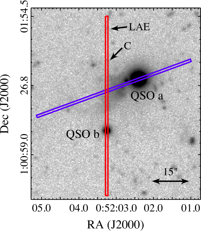
Figure 1.— 10-hours narrow-band image matching the Ly$\alpha$ line at the redshift of UM287 (adapted from Figure 1 of Cantalupo et al. 2014). ‘QSO a’ is the quasar UM287, while ‘QSO b’ is the faint companion quasar . The red and blue lines highlight the position of the 1″slits chosen to study the extended emission in this work. Note that a Lyman Alpha Emitter (‘LAE’) and a continuum source (‘C’) fall within the ‘red’ slit (see Figure 2).

Finally, we flux calibrate our data following the procedure in Hennawi & Prochaska (2013). As standard star spectra were not typically taken immediately before/after our observations, we apply an archived sensitivity function for the LRIS B600/4000 grism to the 1-d extracted quasar spectrum for each slit, and then integrate the flux-calibrated spectrum against the SDSS $g$-band filter curve. The sensitivity function is then rescaled to yield the correct SDSS $g$-band photometry. Since the faint quasar is not clearly detected in SDSS, we only used the $g$-band magnitude of the UM287 quasar to calculate this correction. Note that this procedure is effective for point source flux-calibration because it allows us to account for the typical slit-losses that affect a point source. However, this procedure will tend to underestimate our sensitivity to extended emission, which is not affected by these slit-losses. Hence, our procedure is to apply the rescaled sensitivity functions (based on point source photometry) to our 2-d images, but reduce them by a geometric slit-loss factor so that we properly treat extended emission. To compute the slit-losses we use the measured spatial FWHM to determine the fraction of light going through our $1.0\arcsec$ slits, but we do not model centering errors (see Section §3 for a test of our calibration, and see Hennawi & Prochaska 2013 for more details).

Given this flux calibration, the 1$\sigma$ SB limit of our observations are $SB_{1\sigma}=1.3\times 10^{-18}$ erg s^-1 cm^-2 arcsec^-2, and $SB_{1\sigma}=1.5\times 10^{-18}$ erg s^-1 cm^-2 arcsec^-2 for C IV and He II, respectively. This limits are obtained by averaging over a 3000 km s^-1 velocity interval, i.e. $\pm 1500$ km s^-1 on either side of the systemic redshift of the UM287 quasar, i.e. $z=2.279\pm 0.001$ (McIntosh et al. 1999), at the C IV and He II locations, and a 1″ $\times$ 1″ aperture. This limits (approximately independent of wavelength) are about $3\times$ the $1\sigma$ limit in 1 arcsec² quoted by Cantalupo et al. (2014) for their $\sim 10$ hours narrow-band exposure targeting the Ly$\alpha$ line, i.e. $5\times 10^{-19}$ erg s^-1 cm^-2 arcsec^-2   . Note that we choose this velocity range to enclose all the extended Ly$\alpha$ emission, even after smoothing (see next Section §3), and because the narrow-band image of Cantalupo et al. (2014) covers approximately this width, i.e. $\Delta v\sim 2400$ km s^-1.

Further, it is important to stress here that the line ratios we use in this work are only from the spectroscopic data (we do not use the NB data for the Ly$\alpha$ line), and hence they are independent of any errors in the absolute calibration. Although we do not use the NB data in our analysis, we show in the next section that our results are consistent with the NB imaging, and thus robustly calibrated.

3. Observational Results

Following Hennawi & Prochaska (2013), we search for extended Ly$\alpha$, C IV, and He II emission by constructing a $\chi$ image

$$\chi^{2}=\sum_{i}^{N_{\rm pix}}\frac{\left({\rm DATA}_{i}-{\rm MODEL}_{i}\right)^{2}}{\sigma_{i}^{2}}$$ (1)

where the sum is taken over all $N_{\rm pix}$ pixels in the image, ‘DATA’ is the image, ‘MODEL’ is a linear combination of 2-d basis functions multiplied by B-spline spectral amplitudes, and $\sigma$ is a model of the noise in the spectrum, i.e. $\sigma^{2}={\rm SKY}+{\rm OBJECTS}+{\rm READNOISE}$. The ‘MODEL’ and the $\sigma^{2}$ are obtained during our data reduction procedure (see Section §2, and Hennawi & Prochaska 2013 for details).

Figures 2 and 3 show the two-dimensional spectra for the slits in Figure 1 plotted as $\chi$-maps. Note that if our noise model is an accurate description of the data, the distribution of pixel values in the $\chi$-maps should be a Gaussian with unit variance. In these images, emission will be manifest as residual flux, inconsistent with being Gaussian distributed noise. The bottom row of each figure shows the $\chi_{\rm sky}$ map (only sky subtracted) at the location of the Ly$\alpha$, C IV, and He II, respectively. Even in these unsmoothed data the extended Ly$\alpha$ emission is clearly visible up to $\sim 200$ kpc ($\sim 24$″) from ‘QSO b’, along the ‘red’ slit (Figure 2). This emission has SB${}_{\rm Ly\alpha}=(6.3\pm 0.4)\times 10^{-18}$ erg s^-1 cm^-2 arcsec^-2, calculated in a 1″$\times$20″aperture and over a 3000 km s^-1 velocity interval (blue box in Figure 2). This value is in agreement with the emission detected in the continuum-subtracted image presented in Cantalupo et al. (2014) within a 1″$\times$20″aperture at the same position within the slit, i.e. SB${}_{\rm Ly\alpha}=(7.0\pm 0.1)\times 10^{-18}$ erg s^-1 cm^-2 arcsec^-2. Along the ’blue’ slit, the extended emission is inevitably mixed with the PSF of the hyper-luminous UM287 QSO, making PSF subtraction much more challenging. Nevertheless, we compute the emission in the extended Ly$\alpha$ line in an aperture of about 1″$\times$13″aperture (from 40 to 150 kpc) and within 3000 km s^-1, after subtracting the PSF of the quasar (see Figure 3). Again, we find that surface brightness measured from spectroscopy (SB${}_{\rm Ly\alpha}=1.4\times 10^{-17}$ erg s^-1 cm^-2 arcsec^-2), and from narrow-band imaging (SB${}_{\rm Ly\alpha}=1.7\times 10^{-17}$ erg s^-1 cm^-2 arcsec^-2) agree within the uncertainties. The agreement between the Ly$\alpha$ spectroscopic and narrow band imaging surface brightnesses for both slit orientations confirm that our spectroscopic calibration procedure is robust.

We do not detect any extended emission in either the C IV or in the He II line, for either of the slit orientations. To better visualize the presence of extended emission, we first subtract the PSF of the QSOs for each position angle (see middle rows in Figures 2, and 3), and finally, we show in the upper rows the smoothed $\chi_{\rm smth}$ maps. These smoothed maps are of great assistance in identifying faint extended emission (see Hennawi & Prochaska 2013 for more details on the PSF subtraction and the calculation of the smoothed $\chi$-maps). The lack of compelling emission features in the PSF-subtracted smoothed maps confirm the absence of extended C IV and He II at our sensitivity limits in both slit orientations.

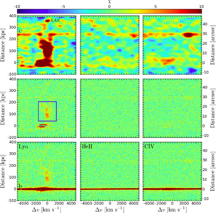
Figure 2.— Two-dimensional spectra for the red slit shown in Figure 1, plotted as $\chi$-maps following Hennawi & Prochaska (2013). In all panels, $v=0$ km s^-1 indicates the systemic redshift of the UM287 quasar, while the distance is computed from the companion quasar, i.e. ‘QSO b’. Bottom row: $\chi_{\rm sky}$ (sky-subtracted only) at the location of Ly$\alpha$, He II, and C IV. Middle row: $\chi_{\rm sky+PSF}$ (sky and PSF subtracted) at the location of Ly$\alpha$, He II, and C IV. Upper row: smoothed maps $\chi_{\rm smth}$ after the PSF subtraction of the companion QSO (‘QSO b’ in Figure 1). As expected, the extended Ly$\alpha$ emission is well visible in these panels up to 200 kpc from the companion QSO. Note also that within this slit we have a continuum source (source ‘C’ in Figure 1) at $\sim 230$ kpc, and a Lyman Alpha emitter (‘LAE’, also highlighted in Figure 1) at $\sim 350$ kpc (see Section §3 for details). The blue box indicates the aperture used to compute the SB_Lyα, and the limits on He II/Ly$\alpha$ and C IV/Ly$\alpha$ line ratios, i.e. 1″$\times$20″and $\Delta v=3000$ km s^-1.

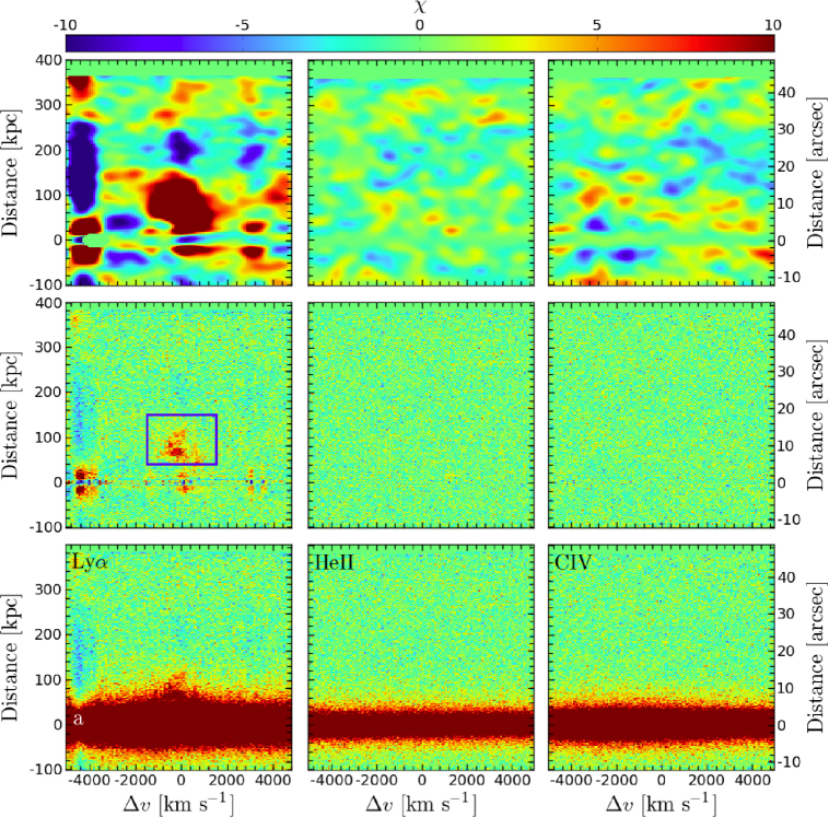
Figure 3.— Two-dimensional spectra for the blue slit shown in Figure 1, plotted as $\chi$-maps following Hennawi & Prochaska (2013). In all panels, $v=0$ km s^-1 indicates the systemic redshift of the UM287 quasar. The distance is also computed from the UM287 quasar, i.e. ‘QSO a’. Bottom row: $\chi_{\rm sky}$ (sky-subtracted only) at the location of Ly$\alpha$, He II, and C IV. Middle row: $\chi_{\rm sky+PSF}$ (sky and PSF subtracted) at the location of Ly$\alpha$, He II, and C IV. Upper row: smoothed maps $\chi_{\rm smth}$ after the PSF subtraction of the UM287 QSO (‘QSO a’ in Figure 1). As expected, also along this slit we detect extended Ly$\alpha$ emission. Given our sensitivity limits, the Ly$\alpha$ line is detected up to $\sim$150 kpc from the UM287 QSO. Note that for such a bright QSO, it is difficult to cleanly subtract its PSF. The blue box indicates the aperture used to compute the SB_Lyα as outlined in section §3.

As our goal is to measure line ratios between the Ly$\alpha$ emission and the C IV and He II lines, we compute the surface brightness limits within the same aperture in which we calculated the Ly$\alpha$ emission along the ’red’ slit, i.e. 1″$\times$20″and $\Delta v=3000$ km s^-1. Because the companion quasar is much fainter than the UM287 quasar, the PSF subtraction along the ‘red’ slit does not suffer from systematics, whereas the large residuals in the left panel of Figure 3 indicate that there are significant PSF subtraction systematics for the Ly$\alpha$ emission in the ‘blue’ slit covering the UM287 quasar. We have thus decided to focus on the line ratios obtained from the ‘red’ slit, although the constraints we obtain from the ‘blue’ slit are comparable. We find SB${}_{1\sigma,CIV}^{A=20}=3.3\times 10^{-19}$ erg s^-1 cm^-2 arcsec^-2 and SB${}_{1\sigma,HeII}^{A=20}=3.7\times 10^{-19}$ erg s^-1 cm^-2 arcsec^-2, respectively at the CIV and HeII locations.

To better understand how well we can recover emission in the He II and C IV lines in comparison to the Ly$\alpha$, we visually estimate the detectability of extended emission in these lines by inserting fake sources as follows. First, we select the Ly$\alpha$ emission above its local $1\sigma$ limit along the ‘red’ slit, we smooth it and scale it to be 1, 2, 3, and 5$\times$ SB${}_{1\sigma}^{A=20}$ at the location of the HeII and CIV line. Finally, we add Poisson realizations of these scaled models into our 2-d PSF and sky-subtracted images. In Figure 4 we show the $\chi$-maps for this test at the location of HeII. This test suggests that we should be able to clearly detect extended emission on the same scale as the Ly$\alpha$ line if the source is $\gtrsim 3\times$ SB${}_{1\sigma}^{A=20}$. Thus, in the remainder of the paper we use 3$\sigma$ ($\sigma\equiv$SB${}_{1\sigma}^{A=20}$) upper limits on the He II/Ly$\alpha$ and C IV/Ly$\alpha$ ratios. Given the values for the SB_Lyα and the surface brightness limits at the location of the CIV and HeII lines (within the 1″$\times$20″aperture and 3000 km s^-1 velocity window for the red slit) we get (He II/Ly$\alpha$)${}_{3\sigma}\lesssim 0.18$ and (C IV/Ly$\alpha$)${}_{3\sigma}\lesssim 0.16$. Note that given the brighter Ly$\alpha$ emission at the location of the ‘blue’ slit, the limits implied are about 2$\times$ lower than these quoted limits for the ‘red’ slit.

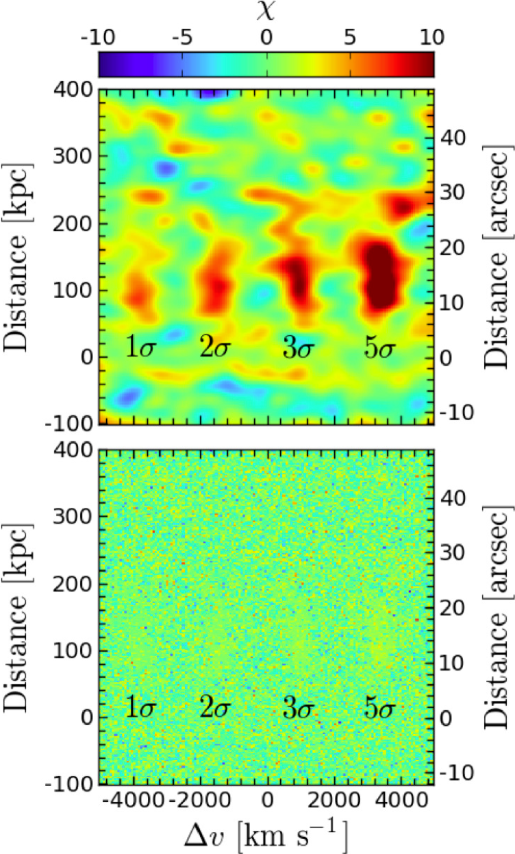
Figure 4.— Illustration of detection significance of scaled models of the Ly$\alpha$ emission at the location of the HeII line along the ‘red’ slit (Figure 2). The synthetic sources corresponds to 1, 2, 3, and 5$\times$ SB${}_{1\sigma,HeII}^{A=20}$. The bottom panel shows the $\chi_{\rm sky}$ (sky-subtracted only) map, while the upper panel shows the smoothed map. This figure suggests that we should be able to clearly detect extended emission $\gtrsim 3\sigma$ on the scale of the Ly$\alpha$ line.

It is important to note that we detect extended C IV emission around the faint companion quasar ‘b’ (see the smoothed maps in Figure 2). As this line is physically distinct from the UM287 nebula and essentially follows the extended Ly$\alpha$ emission around the faint quasar (compare the smoothed maps for Ly$\alpha$ and C IV), this suggests that we have detected the extended narrow emission line region (EELR) of this source. This kind of emission, produced by the gas excited by an AGN on scales of tens of kpc, is usually observed around low redshift $z<0.5$ type-I (e.g. Stockton et al. 2006; Husemann et al. 2013) and type-II quasars (e.g. Greene et al. 2011), traced by [O III] and Balmer lines. We do not quote a value for the emission because, given the much smaller scales in play here, its accuracy depends on the PSF-subtraction. However note that this detection, near the limit of our sensitivity, clearly demonstrates that we could have detected faint extended emission in the C IV and He II lines within the Ly$\alpha$ nebula itself if this emission were characterized by higher line ratios.

Finally, we briefly comment on the nature of two other sources which fall within the ‘red’ slit, i.e. a Lyman Alpha emitter (LAE) (i.e. $EW_{{\rm Ly}\alpha}^{rest}>20$Å) and a continuum source (see Figure 2). Indeed, this slit orientation was also chosen to confirm the presence of a LAE at about 350 kpc northward of ‘QSO b’, clearly visible in the narrow-band image in Figure 2 of Cantalupo et al. (2014) and in our Figure 1. Our LRIS data confirm the presence of a line emission from a LAE at a redshift $z=2.280\pm 0.002$, which is consistent with the redshift of the UM287 quasar, within our uncertainties. We ascribe this emission to the Ly$\alpha$ line, and we compute a flux of $F_{Ly\alpha}=(9.2\pm 0.9)\times 10^{-18}$ erg s^-1 cm^-2 (in an aperture of $\Delta v=1400$ km s^-1, and 4 arcsec²), in agreement with $F_{Ly\alpha}=(8.4\pm 0.4)\times 10^{-18}$ erg s^-1 cm^-2 computed in an aperture of 4 arcsec² in the map of Cantalupo et al. (2014). We also serendipitously obtained a spectrum of a source at $\sim 230$ kpc from quasar ‘b’, which coincides with a continuum sources in our deep V-band image (Cantalupo et al. 2014). In our 2-d spectrum, we detect a faint continuum associated with this source and an emission line at a wavelength of 5123Å, which appears at a velocity $\sim 2750$ km s^-1 from the C IV line in the right panel of Figure 2. However, given the low signal-to-noise ratio of the continuum, and the detection of a single emission line, we are unable to determine the redshift of this source.

3.1. Kinematics of the Nebula

With these slit spectra for two orientations, we can begin to study the kinematics of the Ly$\alpha$ emission of the UM287 giant nebula. We first focus on the ‘red’ slit (see Figure 2), which covers the companion quasar (‘QSO b’) and the extended Ly$\alpha$ emission at a projected distance of $100$$-160$ kpc ($\sim 13$″$-19$″) from UM287 (‘QSO a’). We tested the kinematics of the detected emission by measuring the flux-weighted line centroid and the flux-weighted velocity dispersion ($\sigma$) around the centroid velocity in 2-pixels wide bins ($\sim 0.54$″) across the spatial slit direction. We then converted the velocity dispersion to a gaussian-equivalent FWHM_gauss assuming FWHM${}_{\rm gauss}\sim 2.35\sigma$. Note that, because of the resonant nature of the Ly$\alpha$ emission, the line width may be broadened by radiative transfer effects (e.g., Cantalupo et al. 2005) and representing, thus, only an upper limit for the thermal or kinematical broadening. The extended emission has an average FWHM${}_{\rm gauss}\sim 500$ km s^-1 at a redshift of $z=2.279$, which is centered on the systemic redshift of the UM287 quasar. Although the emission appears coherent on this large scales, the gaussian FWHM calculated at each location ranges between $\sim 370$ km s^-1 and $\sim 600$ km s^-1, suggesting the need of higher resolution data to better characterize its width and shape. The line emission is red-shifted by $\sim 750$ km/s from quasar ‘b’. However note that our estimate for the redshift of quasar ‘b’ $z=2.275$ has a large 800 km s^-1 error, because it is estimated from broad rest-frame UV emission lines which are poor tracers of the systemic frame (Cantalupo et al. 2014).

As for the ‘blue’ slit, statements about kinematics are limited by the challenge of accurately subtracting the PSF of the bright UM287 quasar. Given our SB limit, we detect the Ly$\alpha$ emission out to $\sim 150$ kpc. As expected from the narrow-band imaging, the Ly$\alpha$ is stronger at this location in comparison with the other slit orientation. In particular, the emission shows a peak at $\sim$$63$ kpc ($\sim 7.7$″) in agreement with the narrow-band data (see Figure 1 or Figure 2 in Cantalupo et al. 2014). At this second location, the Ly$\alpha$ line appears broader ${\rm FWHM}_{\rm gauss}\sim 920$ km s^-1 and appears to vary more with distance along the slit. This larger width may arise from the fact we are probing smaller distances from the UM287 quasar than in the ‘red’ slit.

Note that, at our spectral resolution (${{\rm FWHM}\sim 320}$ km s^-1), there is no evidence for “double-peaked” kinematics characteristic of resonantly-trapped Ly$\alpha$ (e.g. Cantalupo et al. 2005) along either slit. This may indicate that resonant scattering of Ly$\alpha$ photons does not play an important role in the Ly$\alpha$ kinematics, however, data at a higher resolution are needed to confirm this conclusion.

These estimates for the widths of Ly$\alpha$ emission are comparable to the velocity widths observed in absorption in the CGM surrounding $z\sim 2$ quasars (${\Delta v\approx 500}$ km s^-1; Prochaska & Hennawi 2009; Lau et al. 2015), pheraps suggesting that the kinematics traced in emission are dominated by the motions of the gas as opposed to the effects of radiative transfer. Both the emission and absorption kinematics are comparable to the virial velocity $\sim 300$ km s^-1 of the massive dark matter halos hosting quasars (M${}_{\rm DM}\sim 10^{12.5}$ M_⊙, White et al. 2012), and thus appear consistent with gravitational motions.

4. Modeling the Ly$\alpha$, CIV and HeII Emission around UM287

As shown by Cantalupo et al. (2014), the extended Ly$\alpha$ emission nebula around UM287 can be explained by photoionization from the central quasar, implying a large amount of cool ($T\sim 10^{4}$ K) gas, i.e. ${M_{c}\simeq 10^{12}\,C^{-1/2}}$ M_⊙. To further constrain the properties of the gas in this huge nebula, in this section we exploit the simple model for cool clouds in a quasar halo introduced by Hennawi & Prochaska (2013) and the consequent photoionization modeling procedure introduced by Arrigoni Battaia et al. (2014b). Our main goal is to show how our line ratio constraints on C IV/Ly$\alpha$ and He II/Ly$\alpha$ can be used to constrain the physical properties of the gas in the UM287 nebula, such as the volume density ($n_{\rm H}$), column density ($N_{\rm H}$), and gas metallicity ($Z$).

We reiterate that as in our previous work (Cantalupo et al. 2014), model the Ly$\alpha$ emission alone cannot break the degeneracy between the clumpiness or density of the gas, and the total gas mass. In the next sections we show how information on additional lines (in particular He II) can constrain the density of the emitting gas and thus break this degeneracy.

4.1. Photoionization Modeling

In the following, we briefly outline the simple model for cool halo gas introduced by Hennawi & Prochaska (2013) for the case of UM287. We assume a simple picture where UM287 has a spherical halo populated with spherical clouds of cool gas ($T\sim 10^{4}$ K) at a single uniform hydrogen volume density $n_{\rm H}$, and uniformly distributed throughout the halo. We model a scale length of $R=160$ kpc from the central quasar, which approximately corresponds to the distance probed by the ‘red’ slit, and represents the expected virial radius for a dark matter halo hosting a quasar at this redshift. In this configuration, the spatial distribution of the gas is completely specified by $n_{\rm H}$, $R$, the hydrogen column density $N_{\rm H}$, and the cloud covering factor $f_{C}$.

Note that the total mass of cool gas in our simple model can be written as (Hennawi & Prochaska 2013):

$$M_{\rm c} = \pi R^{2}f_{\rm C}N_{\rm H}\frac{m_{p}}{X}$$

$$= 2.7\times 10^{10}\!\left(\frac{R}{160\,{\rm kpc}}\right)^{2}\!\!\left(\frac{N_{\rm H}}{10^{19.5}\,{\rm cm}^{-2}}\right)\!\!\left(\frac{f_{\rm C}}{1.0}\right)\,M_{\odot}$$

where $m_{p}$ is the mass of the proton and $X$ is the hydrogen mass fraction.

In this simple model, the Ly$\alpha$ SB is determined by simple relations which depend only on $n_{\rm H}$, $N_{\rm H}$, $f_{C}$, and the luminosity of the QSO at the Lyman limit ($L_{\nu_{\rm LL}}$)(see Hennawi & Prochaska 2013 for details). To build intuition, it is useful to consider two limiting regimes for the recombination emission, for which the clouds are optically thin ($N_{\rm HI}\ll 10^{17.2}$ cm^-2) and optically thick ($N_{\rm HI}\gg 10^{17.2}$ cm^-2) to the Lyman continuum photons, where $N_{\rm HI}$ is the neutral column density of a single spherical cloud. We argue below, that given the luminosity of the UM287 quasar, the optically thick case is however unrealistic.

• Optically thin to the ionizing radiation:

  $${\rm SB}_{{\rm Ly}\alpha}^{\rm thin}=\frac{\eta_{\rm thin}h\nu_{{\rm Ly}\alpha}}{4\pi(1+z)^{4}}~{}\alpha_{\rm A}\left(1+\frac{Y}{2X}\right)n_{\rm H}f_{\rm C}N_{\rm H},$$ (3)

  where $\eta_{\rm thin}=0.42$ is the fraction of recombinations which result in a Ly$\alpha$ photon in the optically thin limit (Osterbrock & Ferland 2006), $h$ is the Planck constant, $\nu_{{\rm Ly}\alpha}$ is the frequency of the Ly$\alpha$ line, $\alpha_{\rm A}=4.18\times 10^{-13}\,{\rm cm^{-3}\,s^{-1}}$ is the case A recombination coefficient at $T=10,000$ K (Osterbrock & Ferland 2006), and $X=0.76$ and $Y=0.24$ are the respective hydrogen and helium mass fractions implied by Big Bang Nucleosynthesis (Boesgaard & Steigman 1985; Izotov et al. 1999; Iocco et al. 2009; Planck Collaboration et al. 2014).

• Optically thick to the ionizing radiation

  $${\rm SB}_{{\rm Ly}\alpha}^{\rm thick}=\frac{\eta_{\rm thick}h\nu_{{\rm Ly}\alpha}}{4\pi(1+z)^{4}}f_{\rm C}\Phi_{\rm LL}\left(R/\sqrt{3}\right),$$ (4)

  where $\eta_{\rm thick}=0.66$ is the fraction of ionizing photons converted into Ly$\alpha$ photons, and where $\Phi_{\rm LL}$ $({\rm[phot\ s^{-1}\ cm^{-2}}])$ is the ionizing photon number flux,

  $$\Phi_{\rm LL}=\int_{\nu_{\rm LL}}^{\infty}\frac{F_{\nu}}{h\nu}d\nu=\frac{1}{4\pi r^{2}}\int_{\nu_{\rm LL}}^{\infty}\frac{L_{\nu}}{h\nu}d\nu.$$ (5)

Thus, in the optically thick case the Ly$\alpha$ surface brightness scales with the luminosity of the central source, $SB_{{\rm Ly}\alpha}^{\rm thick}\propto f_{C}L_{\nu_{\rm LL}}$, while in the optically thin regime the SB does not depend on $L_{\nu_{\rm LL}}$, $SB_{{\rm Ly}\alpha}^{\rm thin}\propto f_{C}n_{\rm H}N_{\rm H}$, provided the AGN is bright enough to keep the gas in the halo ionized enough to be optically thin.

We now argue that the Ly$\alpha$ emitting gas is unlikely to be optically thick $N_{\rm HI}\gtrsim 10^{17.2}$ cm^-2. Equations 4 and 5 can be combined to express the SB in terms of $L_{\nu_{\rm LL}}$, the luminosity at the Lyman edge. To compute this luminosity, we assume that the quasar spectral energy distribution obeys the power-law form $L_{\nu}=L_{\nu_{\rm LL}}(\nu/\nu_{\rm LL})^{\alpha_{\rm UV}}$, blueward of $\nu_{\rm LL}$ and adopt a slope of $\alpha_{\rm UV}=-1.7$ consistent with the measurements of Lusso et al. (2015). The quasar ionizing luminosity is then parameterized by $L_{\nu_{\rm LL}}$, the specific luminosity at the Lyman edge. We determine the normalization $L_{\nu_{\rm LL}}$ by integrating the Lusso et al. (2015) composite spectrum against the SDSS filter curve, and choosing the amplitude to give the correct $i$-band magnitude of the UM287 quasar ($i$-mag$=17.28$), which gives a value of $L_{\nu_{\rm LL}}=5.4\times 10^{31}$ erg s^-1 Hz^-1.

Substituting this value of $L_{\nu_{\rm LL}}$ for UM287 into equation 4, we thus obtain

$${\rm SB}_{{\rm Ly}\alpha}^{\rm thick} = 8.8\times 10^{-16}\left(\frac{1+z}{3.279}\right)^{-4}\!\!\left(\frac{f_{\rm C}}{1.0}\right)\!\!\left(\frac{R}{160\,{\rm kpc}}\right)^{-2}$$

$$\times \left(\frac{L_{\nu_{\rm LL}}}{10^{31.73}\,{\rm erg\,s^{-1}\,Hz^{-1}}}\right){\rm\,erg\,s^{-1}\,cm^{-2}\,arcsec^{-2}}.$$

This value is over two order of magnitude larger than the observed SB value of the Ly$\alpha$ emission at 160 kpc from UM287. Even if we consider a larger radius, $R=250$ kpc, in order to get the observed $SB_{{\rm Ly}\alpha}$ we would need a very low covering factor, i.e. $f_{\rm C}\sim 0.02$. Such a small covering factor would be strictly at odds with the observed smooth morphology of the diffuse nebula as seen in Figure 1. We directly test this assumption as follows. We randomly populate an area comparable to the extent of the Ly$\alpha$ nebula with point sources such that $f_{C}=0.1-1.0$, and we convolve the images with a Gaussian kernel with a FWHM equal to our seeing value, in order to mimic the effect of seeing in the observations. We find that the smooth morphology observed cannot be reproduced by images with $f_{C}<0.5$, as they appear too clumpy. Thus, the smooth morphology of the emission in the Ly$\alpha$ nebula implies a covering factor of $f_{C}\gtrsim 0.5$.

In the following sections we construct photoionization models for a grid of parameters governing the physical properties of the gas to estimate the expected He II and C IV emission. Following the discussion here, we shall see that the models which reproduce the observed Ly$\alpha$ SB will be optically thin, because given the high covering factor optically thick models would be too bright.

4.2. The Impact of Resonant Scattering

It is important to stress at this point that the Ly$\alpha$ photons should be subject to substantial resonant scattering under most of the astrophysical conditions, given the large optical depth at line center (see e.g. Gould & Weinberg 1996). Thus, typically, a Ly$\alpha$ photon experiences a large numbers of scattering before escaping the system in which it is produced. This process thus leads to double-peaked emission line profiles as Ly$\alpha$ photons must diffuse in velocity space far from the line center to be able to escape the system (e.g. Neufeld 1990; Gould & Weinberg 1996; Cantalupo et al. 2005; Dijkstra et al. 2006b; Verhamme et al. 2006). Although our models are optically thin at the Lyman limit, i.e. to ionizing photons, for the model parameters required to reproduce the SB of the emission, they will almost always be optically thick to the Ly$\alpha$ transition (i.e. $N_{\rm HI}\gtrsim 10^{14}$ cm^-2). Hence one should be concerned about the resonant scattering of Ly$\alpha$ photons produced by the central quasar itself. However, radiative transfer simulations of radiation from the UM287 quasar through a simulated gas distribution have shown that the scattered Ly$\alpha$ line photons from the quasar do not contribute significantly to the Ly$\alpha$ surface brightness of the nebula on large scales, i.e. $\gtrsim 100$ kpc (Cantalupo et al. 2014). This is because the resonant scattering process results in very efficient diffusion in velocity space, such that the vast majority of resonantly scattered photons produced by the quasar itself escape the system at very small scales $\lesssim 10$ kpc, and hence do not propagate at larger distances (e.g. Dijkstra et al. 2006b; Verhamme et al. 2006; Cantalupo et al. 2005). For this reason, based on the results of the radiative transfer simulations of Cantalupo et al. (2014), we do not model the contribution of resonant scattering of the quasar photons to the Ly$\alpha$ emission. Similar considerations also apply to the resonant C IV line, however we note that resonant scattering of C IV is expected to be much less efficient, because the much lower abundance of metals imply the gas in the nebula is much less likely to be optically thick to C IV.

To avoid a contribution to the Ly$\alpha$ and C IV emission from scattering of photons from the QSO we have thus masked both lines in our assumed input quasar spectrum. Note that with this approach we do not neglect the ‘scattered’ Ly$\alpha$ photons arising from the diffuse continuum produced by the gas itself, which however turn out to be insignificant .

4.3. Modeling the UM287 Quasar SED

We assume that the spectral energy distribution (SED) of UM287 has the form shown in Figure 5. As we do not have complete coverage of the spectrum of this quasar, we adopt the following assumptions to model the full SED. Given the ionization energies for the species of interest to us in this work, i.e. 1 Ryd=13.6 eV for Hydrogen, 4 Ryd=54.4 eV for He II, and 64.5 eV for C IV, we have decided to stick to power-law approximations above 1 Ryd. However, note that the UV range of the SED is so far not well constrained (see Lusso et al. 2015 and reference therein). In particular, we model the quasar SED using a composite quasar spectrum which has been corrected for IGM absorption (Lusso et al. 2015). This IGM corrected composite is important because it allows us to relate the $i$-band magnitude of the UM287 quasar to the specific luminosity at the Lyman limit $L_{\nu_{\rm LL}}$. For energies greater than one Rydberg, we assume a power law form $L_{\nu}=L_{\nu_{\rm LL}}(\nu/\nu_{\rm LL})^{\alpha_{\rm UV}}$ and adopt a slope of $\alpha_{\rm UV}=-1.7$, consistent with the measurements of Lusso et al. (2015), while in the Appendix we test also the cases for $\alpha_{\rm EUV}=-1.1$, and $-2.3$. We determine the normalization $L_{\nu_{\rm LL}}$ by integrating the Lusso et al. (2015) composite spectrum against the SDSS filter curve, and choosing the amplitude to give the correct $i$-band magnitude of the UM287 quasar (i.e. $i$=17.28), which gives a value of $\L_{\nu_{LL}}=5.4\times 10^{31}$ erg s^-1 Hz^-1. We extend this UV power law to an energy of 30 Rydberg, at which point a slightly different power law is chosen $\alpha=-1.65$, such that we obtain the correct value for the specific luminosity at 2 keV $L_{\nu}({\rm 2\,keV})$ implied by measurements of $\alpha_{\rm OX}$, defined to be $L_{\nu}(2\,{\rm keV})/L_{\nu}(2500\,{\rm\AA})\equiv(\nu_{\rm 2\,keV}/\nu_{2500\,{\rm\AA}})^{\alpha_{\rm OX}}$. We adopt the value $\alpha_{\rm OX}=-1.5$ measured by Strateva et al. (2005) for SDSS quasars. An X-ray slope of $\alpha_{\rm X}=-1$, which is flat in $\nu f_{\nu}$ is adopted in the interval of 2-100 keV, and above 100 keV, we adopt a hard X-ray slope of $\alpha_{\rm HX}=-2$. For the rest-frame optical to mid-IR part of the SED, we splice together the composite spectra of Lusso et al. (2015), Vanden Berk et al. (2001), and Richards et al. (2006). These assumptions about the SED are essentially the standard ones used in photoionization modeling of AGN (e.g. Baskin et al. 2014). Summarizing, given the lack of information, for energies greater than one Rydberg we parametrized the SED of the UM287 quasar with a series of power-laws as

$$f_{\nu}\propto\begin{cases}\nu^{\alpha_{\rm EUV}},&\text{if }h\nu\geq 1\,{\rm Ryd}\\ \nu^{\alpha},&\text{if }30\,{\rm Ryd}\leq h\nu<2\,{\rm keV}\\ \nu^{\alpha_{\rm X}},&\text{if }2\,{\rm keV}\leq h\nu<100\,{\rm keV}\\ \nu^{\alpha_{\rm HX}},&\text{if }h\nu\geq 100\,{\rm keV}.\end{cases}$$ (7)

4.4. Input Parameters to Cloudy

Having established our assumptions on the UM287 SED, and on the resonant scattering, we now explain how we choose the range of our model parameter grid. We perform our calculations with the Cloudy photoionization code (v10.01), last described by Ferland et al. (2013). Because the emitting clouds are expected to be much smaller than their distance $r\sim R_{\rm vir}=160\,{\rm kpc}$ from the central ionizing source, we assume a standard plane-parallel geometry for the emitting clouds illuminated by the distant quasar. In order to keep the models as simple as possible, and because we are primarily interested in understanding how photoionization together with the observed line ratios can constrain the physical properties of the gas (i.e. $n_{\rm H}$ and $N_{\rm H}$), without resorting to extreme parameter combinations, we proceed as follows. We focus on reproducing the SB${}_{\rm Ly\alpha}\sim 7\times 10^{-18}$ erg s^-1 cm^-2 arcsec^-2 at 160 kpc distance from the UM287 quasar, which is basically the distance probed by the ‘red’ slit. In particular, eqn. (3) implies that a certain combination of $N_{\rm H}$ and $n_{\rm H}$ are thus required. Further, given the dependence on metallicity ($Z$) of the C IV and He II lines, and of the gas temperature which determine the amount of collisional excitation in the Ly$\alpha$ line, we also consider variations in $Z$. Thus, we run a uniform grid of models with this wide range of parameters:

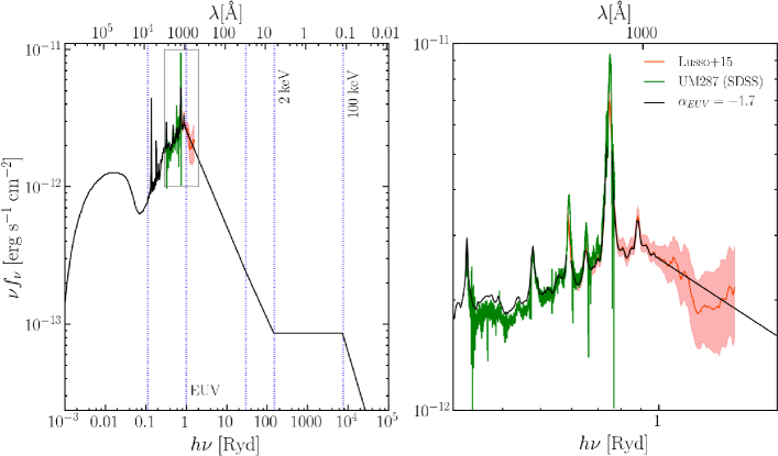
Figure 5.— Spectral energy distribution (SED) of UM287 used as incident radiation field in our modeling. The black solid line indicate our fiducial input spectrum characterized by a slope in the EUV of $\alpha_{\rm EUV}=-1.7$ (Lusso et al. 2015). The right panel is a zoomed version of the box highlighted in the left panel. Note the agreement between the composite spectrum used as input in our calculation and the SDSS spectrum of UM287 (green solid line). To prevent a contribution from resonantly scattered photons, we mask the emission from the line center of Ly$\alpha$ and C IV.

• $n_{\rm H}=10^{-2}$ to 10² cm^-3 (steps of 0.2 dex);

• $N_{\rm H}=10^{18}$ to $10^{22}$ (steps of 0.2 dex);

• $Z=10^{-3}\,Z_{\odot}$ to $Z_{\odot}$ (steps 0.2 dex).

Note that by exploring this large parameter range, some of the models that we consider result in clouds optically thick at the Lyman limit, but as explained in the previous Section §4.1, these parameter combinations result in nebulae which are too bright and thus inconsistent with the observed Ly$\alpha$ surface brightness. In what follows, we only consider the models which closely reproduce the observed Ly$\alpha$ surface brightness, i.e. $5.5\times 10^{-18}$ erg s^-1 cm^-2 arcsec^-2 $<$ SB${}_{\rm Ly\alpha}<8.5\times 10^{-18}$ erg s^-1 cm^-2 arcsec^-2.

Photoionization models are self-similar in the ionization parameter $U\equiv\frac{\Phi_{LL}}{cn_{\rm H}}$, which is the ratio of the number density of ionizing photons to hydrogen atoms. As the luminosity of the central QSO is known, the variation in the ionization parameter $U$ results from the variation of the volume number density $n_{\rm H}$ for the models in our grid. The range of ionization parameters that we cover is comparable to those in previous analysis of photoionization around AGNs, e.g. in the case of the narrow line regions (NLR; e.g. Groves et al. 2004) and in the case of extended emission line regions (EELR; e.g. Humphrey et al. 2008). Finally, we emphasize that once we fix the source luminosity and define the ionizing spectrum, the line ratios we consider are described by two model parameters, namely the density $n_{\rm H}$ of the gas and its metallicity $Z$. We will see this explicitly in the next section.

5. Models vs Observations

As we discuss in Section §3, our LRIS observations provide upper limits on the C IV/Ly$\alpha$ and He II/Ly$\alpha$ ratios, i.e. (C IV/Ly$\alpha$)${}_{3\sigma}\lesssim 0.16$ and (He II/Ly$\alpha$)${}_{3\sigma}\lesssim 0.18$. On the other hand, each photoionization model in our grid predicts these line ratios, and Figure 6 shows the trajectory of these models in the He II/Ly$\alpha$ vs C IV/Ly$\alpha$ plane. The region allowed given our observational constraints on the line ratios is indicated by the green shaded area. We remind the reader that we select only the models which produce the observed Ly$\alpha$ emission of SB${}_{\rm Ly\alpha}\sim 7\times 10^{-18}$ erg s^-1 cm^-2 arcsec^-2, which to lowest order requires a combination of $N_{\rm H}$ and $n_{\rm H}$ as shown by eqn. (3). Since the luminosity of the central source is known, these models can be thought to be parametrized by either $n_{\rm H}$ or the ionization parameter $U$, as shown by the color coding on the color-bar. In the same plot we show trajectories for different metallicities $Z=1,$ $0.1,$ $0.01,$ $10^{-3}\,Z_{\odot}$.

We now reconsider the covering factor. We argued in §4.1 that based on the morphology of the nebula, the covering factor need to be $f_{\rm C}\gtrsim 0.5$, and that optically thick gas clouds would tend to overproduce the Ly$\alpha$ SB for such high covering factors. Our models provide a confirmation of this behavior. For a covering factor of $f_{\rm C}=1.0$ a large number of models are available, whereas if we lower the covering factor to $f_{\rm C}=0.3$, we find that only two models in our extensive model grid can satisfy the Ly$\alpha$ SB of the nebula. This results because as we decrease $f_{\rm C}$, assuming the gas is optically thin, eqn. (3) indicates we must correspondingly increase the product $N_{\rm H}n_{\rm H}$ by $1/f_{\rm C}$ in order to match the observed Ly$\alpha$ SB. However, note that the neutral fraction also scales with this product $x_{\rm HI}\propto N_{\rm H}n_{\rm H}$ such that for low enough values of $f_{\rm C}$ increasing $N_{\rm H}n_{\rm H}$ would result in self-shielding clouds that are optically thick. We already argued in §4.1 that if the clouds are optically thick the covering factor must be much lower $f_{\rm C}\simeq 0.02$, which is ruled out by the diffuse morphology of the nebula. Hence our constraint on the covering factor $f_{\rm C}\gtrsim 0.5$ can also be motivated by the simple fact that gas distributions with lower covering factors would over-produce the Ly$\alpha$ SB. Henceforth, for simplicity, we assume a covering factor of $f_{\rm C}=1.0$ throughout this work, but in §7 we test the sensitivity of our results to this assumption.

The gray symbols in Figure 6 also show a compilation of measurements of the He II/Ly$\alpha$ and C IV/Ly$\alpha$ line ratios from the literature for other giant Ly$\alpha$ nebulae from the compilation in Arrigoni Battaia et al. (2014b). Specifically, we show measurements or upper limits for the two line ratios for seven Ly$\alpha$ blobs (Dey et al. 2005; Prescott et al. 2009, 2013; Arrigoni Battaia et al. 2014b), and Ly$\alpha$ nebulae associated with 53 high redshift radio galaxies (Humphrey et al. 2006; Villar-Martín et al. 2007). Note that we show measurements from the literature in Figure 6 for reference, but these measurements cannot be directly compared to our observations or our models for several reasons. First, the emission arising from the narrow line region of the central obscured AGN is typically included for the HzRGs, contaminating the line ratios for the nebulae. In addition, the central source UV luminosities are unknown for both LABs and HzRGs, and thus they cannot be directly compared to our models, which assume a central source luminosity. See Arrigoni Battaia et al. 2014b and references therein for a discussion on this dataset and its caveats.

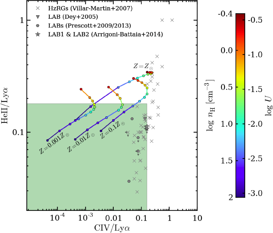
Figure 6.— HeII/Ly$\alpha$ versus CIV/Ly$\alpha$ log-log plot. Our upper limits on the HeII/Ly$\alpha$ and CIV/Ly$\alpha$ ratios are compared with the Cloudy photoionization models that reproduce the observed SB${}_{\rm Ly\alpha}\sim 7\times 10^{-18}$ erg s^-1 cm^-2 arcsec^-2. For clarity, we plot only the models with $Z=0.001,0.01,0.1,$ and $1Z_{\odot}$. The models are color coded following the ionization parameter $U$, and thus the volume density $n_{\rm H}$ (see color bar on the right). The green shaded area represents the region defined by the upper limits of the UM287 nebula. Note that these upper limits favor models with $n_{\rm H}\gtrsim 3$ cm^-3, $N_{\rm H}\lesssim 10^{20}$ cm^-2, and $\log U\lesssim-1.5$. This is even more clear in Figure 7.

The trajectory of our optically thin models through the He II/Ly$\alpha$ and C IV/Ly$\alpha$ diagram can be understood as follows. We first focus on the curve for $Z=Z_{\odot}$ and follow it from low to high $U$ (i.e. from high to low volume density $n_{\rm H}$). First consider the trend of the He II/Ly$\alpha$ ratio. He II is a recombination line and thus, once the density is fixed, its emission depends basically on the fraction of Helium that is doubly ionized. For this reason, the He II/Ly$\alpha$ ratio is increasing from log$U\sim-3$ and ‘saturates’, reaching a peak at a value of $\sim 0.34$ which is set by atomic physics and in particular by the ratio of the recombination coefficients of Ly$\alpha$ and He II. Indeed, if we neglect the contribution of collisional excitation to the Ly$\alpha$ line emission, which is a reasonable assumption near solar metallicity, then both the He II and Ly$\alpha$ are produced primarily by recombination and the recombination emissivity can be written as

$$j_{\rm line}=f_{\rm V}^{\rm elem}\frac{h\nu_{\rm line}}{4\pi}n_{\rm e}n_{\rm ion}\alpha_{\rm line}^{\rm eff}(T),$$ (8)

where $n_{\rm ion}$ is the volume density of He⁺⁺ and H⁺ for the case of HeII and Ly$\alpha$, respectively. Here $\alpha_{\rm line}^{\rm eff}(T)$ is the temperature dependent recombination coefficient for HeII or Ly$\alpha$, and the factor $f_{\rm V}^{\rm elem}=3f_{\rm C}N_{\rm elem}/(4Rn_{\rm elem})$ takes into account that the emitting clouds fill only a fraction of the volume (see Hennawi & Prochaska 2013). Thus, once the Helium is completely doubly ionized, i.e. $n_{\rm p}\sim n_{\rm H}$ and $n_{\rm He^{++}}\sim(Y/2X)n_{\rm H}$, the ratio between the two lines is given by the relation

$$\frac{j_{\rm HeII}}{j_{\rm Ly\alpha}} = 0.34\left(\frac{\alpha_{\rm HeII}^{\rm eff}(20,000K)}{1.15\times 10^{-12}\,{\rm cm^{3}\,s^{-1}}}\right)$$

$$\times \left(\frac{\alpha_{\rm Ly\alpha}^{\rm eff}(20,000K)}{2.51\times 10^{-13}\,{\rm cm^{3}\,s^{-1}}}\right)^{-1},$$

Note that eqn. (5) depends slightly on temperature, with a decrease of the ratio at higher temperatures. Before reaching this maximum line ratio, He II/Ly$\alpha$ is lower because Helium is not completely ionized, and is roughly given by ${{\rm HeII}/{\rm Ly}\alpha\sim x_{\rm He^{++}}\times(j_{\rm HeII}/j_{\rm Ly\alpha})_{\rm max}}$, where $x_{\rm He^{++}}$ is the fraction of doubly ionized Helium. As stated above, this simple argument does not take into account collisional excitation of Ly$\alpha$. In particular, at lower metallicities when metal line coolants are lacking, the temperature of the nebula is increased, and collisionally excited Ly$\alpha$, which is extremely sensitive to temperature, becomes an important coolant, boosting the Ly$\alpha$ emission over the pure recombination value. Thus metallicity variations result in a change of the level of the asymptotic HeII/Lya ratio as seen in Figure 6.

Our photoionization models indicate that the C IV emission line is an important coolant and is powered primarily by collisional excitation. The efficiency of C IV as a coolant depends on the amount of Carbon in the C⁺³ ionic state. For this reason, the C IV/Ly$\alpha$ ratio is increasing from log$U\sim-3$, reaches a peak due to a maximum in the $C^{+3}$ fraction, and lowers again at higher $U$ where Carbon is excited to yet higher ionization states, e.g. C V. For example, for the $Z=0.1\ Z_{\odot}$ models, the C IV/Ly$\alpha$ ratio peaks at log $U=-1.4$ and then decreases at higher $U$. Given that C IV is a coolant, the strength of its emission depends on the metallicity of the gas. Indeed, for metallicities lower than solar, C IV becomes a sub-dominant coolant with respect to collisionally excited Ly$\alpha$ (and for very low metallicity, e.g. $Z=10^{-3}Z_{\odot}$, also to He Ly$\alpha$), and its emission becomes metallicity dependent as can be seen in Figure 6.

At lower metallicities the Ly$\alpha$ line becomes an important coolant. For the $Z=0.001Z_{\odot}$ grid, the collisional contribution to Ly$\alpha$ has an average value of $\sim 40$%, while it decreases to $\sim 37$%, $\sim 25$%, $\sim 1$% for the $Z=0.01,0.1,1\,Z_{\odot}$ cases, respectively. Given that the strength of the collisionally excited Ly$\alpha$ emission increases with density along each model trajectory, this slightly dilutes the aforementioned trends in the He II and C IV line emission. Specifically, the density dependence of collisionally excited Ly$\alpha$ emission moves the line ratios to lower values for log$\,U\gtrsim-1.5$, which would otherwise asymptote at the expected He II/Ly$\alpha$ ratio in eqn. (5). Thus the effect of collisionally excited Ly$\alpha$ emission tend to mask the ‘saturation’ of the He II/Ly$\alpha$ ratio due to recombination effects alone, and results in a continuous increase of He II/Ly$\alpha$ with $U$.

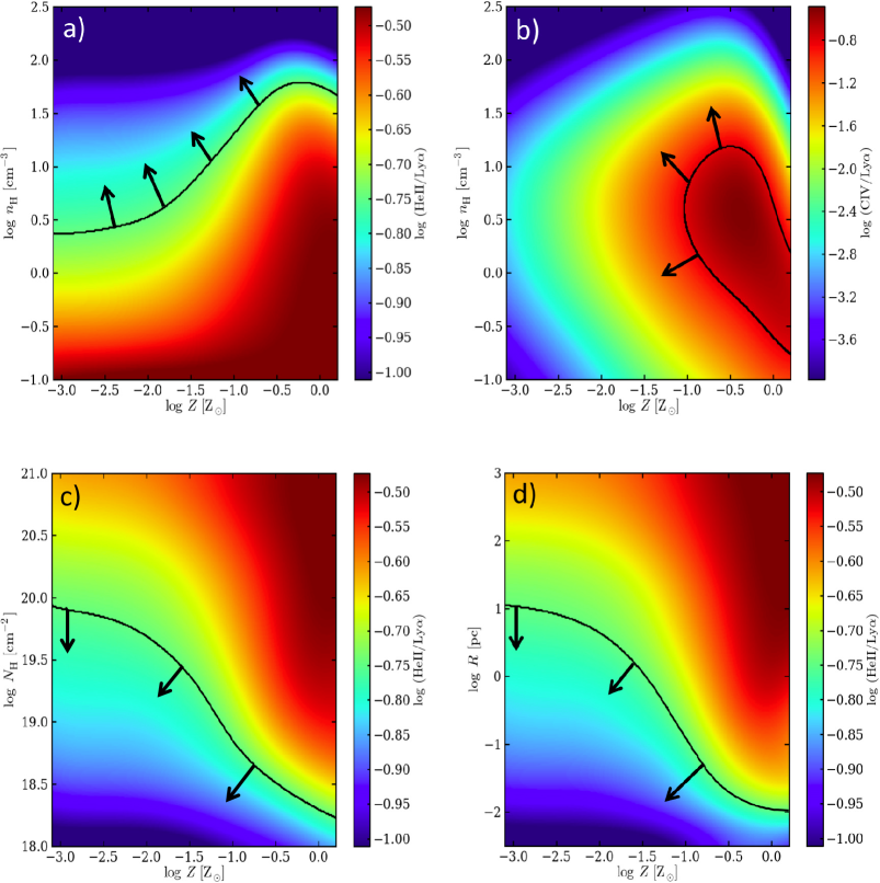
Figure 7.— Constraints on the physical parameters of the gas clouds from our photoionization models that reproduce the observed SB${}_{\rm Ly\alpha}\sim 7\times 10^{-18}$ erg s^-1 cm^-2 arcsec^-2 in the case of an input spectrum with $\alpha_{\rm EUV}=-1.7$. Given the known luminosity of the central source, the assumed SED, and the fixed SB_Lyα, our models can be thought to be parametrized by only two parameters, namely $n_{\rm H}$ and $Z$. Panel ‘a’: map of the He II/Ly$\alpha$ ratio in the $n_{\rm H}$-$Z$ plane. The black solid line indicate our 3$\sigma$ upper limit He II/Ly$\alpha$ $<0.18$ (i.e. log(He II/Ly$\alpha$)$<-0.74$). Panel ‘b’: map of the C IV/Ly$\alpha$ ratio in the $n_{\rm H}$-$Z$ plane. The black solid line indicate our 3$\sigma$ upper limit C IV/Ly$\alpha$ $<0.16$ (i.e. log(He II/Ly$\alpha$)$<-0.79$). Note that the constraints from the He II/Ly$\alpha$ ratio are stronger. Panel ‘c’: map of the He II/Ly$\alpha$ ratio in the $N_{\rm H}$-$Z$ plane. The black solid line indicate our 3$\sigma$ upper limit. Models with $N_{\rm H}\lesssim 10^{20}$ cm^-2 are selected. Panel ‘d’: map of the He II/Ly$\alpha$ ratio in the $R$-$Z$ plane. The black solid line indicate our 3$\sigma$ upper limit. Note that really small cloud sizes are favored, i.e. $R\lesssim 20$ pc.

Overall, Figure 6 illustrates that our simple photoionization models can accommodate the constraints implied by our observed upper limits on the He II/Ly$\alpha$ and C IV/Ly$\alpha$ ratios of UM287. In particular, our non-detections are satisfied (green shaded region) for models with high volume densities $n_{\rm H}$ and low metallicities $Z$. These constraints can be more easily visualized in Figure 7, where we show the allowed regions in the $n_{\rm H}$-$Z$ plane implied by our limits on the He II/Ly$\alpha$ (panel ‘a’) and C IV/Ly$\alpha$ ratios (panel ‘b’). Specifically, in these panels the solid black line indicate the upper limits in the case of the UM287 nebula, i.e. He II/Ly$\alpha$ $<0.18$ (or log(He II/Ly$\alpha$)$<-0.74$), and C IV/Ly$\alpha$ = 0.16 (or log(C IV/Ly$\alpha$)$<-0.79$), while the arrows indicate the region of the parameter space that is allowed. It is evident that our limits on the extended emission in the He II/Ly$\alpha$ ratio give us stronger constraints than those from the C IV/Ly$\alpha$ ratio. The He II/Ly$\alpha$ ratio provides a constraint on the volume density which is metallicity dependent, however even if we assume a $\log_{10}Z\simeq-2-3$, which are the lowest possible values comparable to the background metallicity of the IGM (e.g. Schaye et al. 2003), we obtain a conservative lower limit on the volume density of $n_{\rm H}\gtrsim 3$ cm^-3.

Given this constraint on $n_{\rm H}$, and the fact that we know the Ly$\alpha$ emission level, which in turns approximately scales as $n_{\rm H}N_{\rm H}$ (see eqn. (3)), we can use our lower limit on $n_{\rm H}$ to place an upper limit on $N_{\rm H}$ or equivalently on the total cool gas mass because it scales as $f_{\rm C}\,N_{\rm H}$ once the radius is fixed (see eqn. (4.1)). Panel ‘c’ of Figure 7 shows that our limit on the He II/Ly$\alpha$ ratio combined with the total SB_Lyα implies the emitting clouds have column densities $N_{\rm H}\lesssim 10^{20}$ cm^-2. Thus, if we assume that the physical properties of the slab modeled at 160 kpc are representative of the whole nebula, we can compute a rough estimate for the total cool gas mass. With this strong assumption, that $n_{\rm H}\gtrsim 3$ cm^-3 is valid over the entire area of the nebula, i.e. $911$ arcsec² (from the $2\sigma$ isophote of the Ly$\alpha$ map; Cantalupo et al. 2014), we then deduce that $N_{\rm H}\lesssim 10^{20}$ cm^-2 over this same area, and hence the total cool gas mass is ${M_{\rm c}\lesssim 6.4\times 10^{10}}$ M_⊙.

Further, by combining the lower limit on volume density $n_{\rm H}$ and upper limit on column density $N_{\rm H}$, we can also obtain an upper limit on the sizes of the emitting clouds defined as ${R\equiv N_{\rm H}/n_{\rm H}}$. Panel ‘d’ in Figure 7 shows that this upper limit is constrained to be $R\lesssim 20$ pc. Assuming a unit covering factor $f_{\rm C}=1.0$, this constraint on cloud sizes implies $\gtrsim 53,500$ clouds per square arcsec on the sky, and each cloud should have a cool gas mass $M_{\rm c}\lesssim 1.3\times 10^{3}$ M_⊙. Assuming these clouds have the same properties throughout the whole nebula, we find that $\gtrsim 4.9\times 10^{7}$ clouds are needed to cover the extent of the Ly$\alpha$ emission ($\sim 911$ arcsec²).

The foregoing discussion indicates that we are able to break the degeneracy between the volume density of the gas $n_{\rm H}$ and the total cool gas mass presented in Cantalupo et al. (2014). As a reminder, this degeneracy arises because the Ly$\alpha$ surface brightness scales as ${\rm SB_{{\rm Ly}\alpha}}\propto n_{\rm H}N_{\rm H}$, whereas the total cool gas mass is given by $M_{\rm c}\propto N_{\rm H}$. Thus observations of the Ly$\alpha$ alone cannot independently determine the cool gas mass. Cantalupo et al. (2014) modeled the Ly$\alpha$ emission in the UM287 nebula in a way that differs from our simple model of cool clouds in the quasar CGM. Specifically, they used the gas distribution in a massive dark matter halo $M=10^{12.5}$ M_⊙ meant to represent the quasar host, and carried out ionizing and Ly$\alpha$ radiative transfer simulations under the assumption the gas is highly ionized by a quasar with the same luminosity as UM287, and the extended Ly$\alpha$ emission is dominated by recombinations, similarly to our simpler Cloudy models. Under these assumptions, they are not able to reproduce the observed Ly$\alpha$ surface brightness of the nebula. This arises because only $\sim 15\%$ of the total gas in the simulated halo is cool enough to emit Ly$\alpha$ recombination radiation ($T<5\times 10^{4}$ K), because the vast majority of the baryons in the halo have been shock-heated to the virial temperature of the halo, i.e. $T\sim 10^{7}$ K. Even if they assume all of the gas in the simulated halo can produce the Ly$\alpha$ line ($M_{\rm gas}\approx 10^{11.3}$ M_⊙ for the dark matter halo; Cantalupo et al. 2014), the surface brightness of the resulting nebula is still too faint. As a result, Cantalupo et al. (2014) postulated that the emission in the simulated halo must be boosted by a clumping factor $C=\langle n_{\rm H}^{2}\rangle/\langle n_{\rm H}\rangle^{2}$, which represents the impact of clumps of cool gas which are not resolved by the simulation. They then determined the scaling relation between the simulated Ly$\alpha$ emission and the column density of the simulated gas distribution, i.e. $N_{\rm H}\propto{\rm SB_{{\rm Ly}\alpha}}^{1/2}\,C^{-1/2}$ (Cantalupo et al. 2014), as expected for recombination radiation. Note that accordingly, ${\rm SB_{{\rm Ly}\alpha}}^{1/2}\propto N_{\rm H}\,C^{1/2}\propto M_{\rm c}\,C^{1/2}$ and one sees that this is identical to the scaling implied by eqn. (3), ${\rm SB_{{\rm Ly}\alpha}}\propto N_{\rm H}n_{\rm H}$, if one identifies $n_{\rm H}$ with $C^{1/2}\langle n_{\rm H}\rangle$. Our simple cloud model adopts a single density for all the clouds $n_{\rm H}$, whereas in the clumping picture, there could be a range of densities present, but the emission is dominated by gas with $n_{\rm H}\simeq C^{1/2}\,\langle n_{\rm H}\rangle$. In this context, Cantalupo et al. (2014) inferred that if $C=1$, the high observed SB_Lyα, implies very high column densities up to $N_{\rm H}\approx 10^{22}$ cm^-2 corresponding to cool gas masses $M_{\rm c}=10^{12}$ M_⊙, in excess of the baryon budget of the simulation. More generally, in the presence of clumping this constraint becomes $M_{\rm c}=10^{12}\,C^{-1/2}$ M_⊙.

By introducing the constraint on the volume density $n_{\rm H}\gtrsim 3$ cm^-3 using the He II/Ly$\alpha$ ratio, our work (i) breaks the degeneracy between density $n_{\rm H}$ (or equivalently $C$) and total column density $N_{\rm H}$ (or equivalently $M_{\rm c}$), (ii) allows us to then constrain the total cool gas mass ${M_{\rm c}\lesssim 6.4\times 10^{10}}$ M_⊙ without making any assumptions about the quasar host halo mass, and (iii) demands the existence of a population of extremely compact ($R\lesssim 20$ pc) dense clouds in the CGM/IGM. The ISM-like densities and extremely small sizes of these clouds clearly indicate that they would be unresolved by current cosmological hydrodynamical simulations, given their resolution on galactic scales (Fumagalli et al. 2014; Faucher-Giguere et al. 2014; Crighton et al. 2015; Nelson et al. 2015). Indeed, our measurements would imply a clumping factor $C\gtrsim 200$ for the simulation of Cantalupo et al. (2014), in agreement with the value they required in order to reproduce the observed Ly$\alpha$ from their simulated halo.

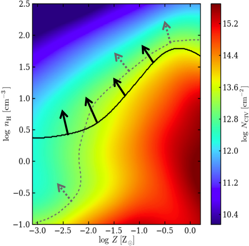
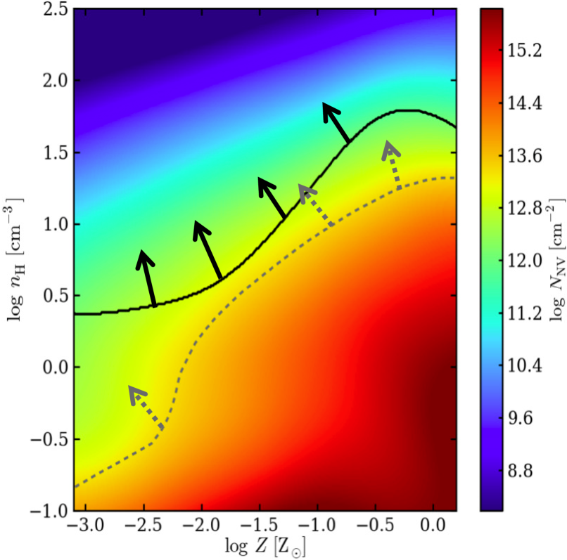
Figure 8.— Top Panel: Map of the C IV column density $N_{\rm CIV}$ in the $n_{\rm H}$-$Z$ plane built from our photoionization models that reproduce the observed SB${}_{\rm Ly\alpha}\sim 7\times 10^{-18}$ erg s^-1 cm^-2 arcsec^-2 in the case of an input spectrum with $\alpha_{\rm EUV}=-1.7$. The black solid line indicate our 3$\sigma$ upper limit in the He II/Ly$\alpha$ ratio, while the gray dashed line indicate our limit of $N_{\rm CIV}<10^{13.2}$ cm^-2 implied by the absence of absorption at the resolution of the SDSS spectrum of UM287. Bottom Panel: Map of the N V column density $N_{\rm NV}$ in the $n_{\rm H}$-$Z$ plane built from our photoionization models that reproduce the observed SB${}_{\rm Ly\alpha}\sim 7\times 10^{-18}$ erg s^-1 cm^-2 arcsec^-2 in the case of an input spectrum with $\alpha_{\rm EUV}=-1.7$. The black solid line indicate our 3$\sigma$ upper limit in the He II/Ly$\alpha$ ratio, while the gray dashed line indicate our limit of $N_{\rm NV}<10^{13.4}$ cm^-2 implied by the absence of absorption at the resolution of the SDSS spectrum of UM287. The spectroscopic constraints for both species imply that the gas along the sightline, if present, is in a similar state as the observed nebula, being illuminated by the bright quasar as well.

5.1. Constraints from Absorption Lines

A source lying in the background of the UM287 nebula that pierces the gas at an impact parameter of $\simeq 160$ kpc may also exhibit absorption from high-ion UV transitions like C IV and N V, which can be constrained from absorption spectroscopy. In Figure 8 we show a map for the column density of the C IV and N V ionic states ($N_{\rm CIV}$, $N_{\rm NV}$) for our model grid that reproduces the observed SB${}_{\rm Ly\alpha}\sim 7\times 10^{-18}$ erg s^-1 cm^-2 arcsec^-2. Given our non-detection of He II emission, our upper limits on the He II/Ly$\alpha$ ratios (indicated by the black solid line in both panels), imply $N_{\rm CIV}\lesssim 10^{13.8}$ cm^-2 and $N_{\rm NV}\lesssim 10^{13.0}$ cm^-2, respectively. The quasar UM287 resides at the center of the nebula, and our narrow band image indicates it is surrounded by Ly$\alpha$ emitting gas. It is thus natural to assume that the UM287 quasar pierces the nebular gas over a range of radial distances. Thus a non-detection of absorption in these transitions places further constraints on the physical state of the absorbing gas in the nebula.

To this end, we examined the high signal-to-noise ${\rm S/N}\simeq$ 70 pix^-1 SDSS spectrum of the UM287 quasar, which has a resolution of $R\simeq 2000$. We find no evidence for any metal-line absorption within a $\sim 2000$ km s^-1 window of the quasar systemic redshift coincident with the velocity of the Ly$\alpha$ emitting nebula (see Figure 2-3), implying $N_{\rm CIV}<10^{13.2}$ cm^-2 (EW${}_{\rm CIV}<15$ mÅ), and $N_{\rm NV}<10^{13.4}$ cm^-2. These limits constrain the amount of gas in these ionic states intercepted by the quasar at all distances, but in particular at $\simeq 160$ kpc, where we conducted our detailed modeling of the emission. As such, directly analogous to our constraints from the emission line ratios, we can similarly determine the constraints in the $n_{\rm H}$-$Z$ plane from the non-detections of C IV and N V absorption, which are shown as the gray dashed lines in Figure 8. As expected these metal absorption constraints depend sensitively on the enrichment of the gas, but the region of the $n_{\rm H}$-$Z$ plane required by our non-detections are consistent with that required by our He II/Ly$\alpha$ emission constraint. Specifically, for log $Z>-2.3$, the absence of absorption provides a comparable lower-limit on the density as the non-detection of emission, whereas at lower metallicities the absorption constraint allows lower volume densities $n_{\rm H}>0.1$ cm^-3 (Figure 8), which are already ruled out by He II/Ly$\alpha$. To conclude, in the context of our simple model, both high-ion metal-line absorption and He II and C IV emission paint a consistent picture of the physical state of the gas.

For completeness, we also searched for metal-line absorption along the companion quasar ‘QSO b’ sightline in our Keck/LRIS spectrum (resolution $R\simeq 1000$ and ${\rm S/N}\simeq 60$ pix^-1). We do detect strong, saturated C IV absorption with $N_{\rm CIV}>10^{14.4}$ cm^-2 and $z=2.2601$. This implies, however, a velocity offset of $\approx-1700$ km s^-1 with respect to the systemic redshift of the UM287 quasar, and thus from the extended Ly$\alpha$ emission detected in the slit spectrum of Figure 2. Given this large kinematic displacement from the nebular Ly$\alpha$ emission, we argue that this absorption is probably not associated with the UM287 nebulae, and is likely to be a narrow-associated absorption line system associated with the companion quasar. This is further supported by the strong detection of the rarely observed N V doublet. The large negative velocity offset $-1370$ km s^-1 between the absorption and our best estimate for the redshift of QSOb $z=2.275$ (from the Si IV emission line) suggests that this is outflowing gas, but given the large error $\sim 800{\rm km\,s^{-1}}$ on the latter, and the unknown distance of this absorbing gas along the line-of-sight, we do not speculate further on its nature.

Finally, note that at the time of writing, there is no existing echelle spectrum of UM287 available, although given that this quasar is hyper-luminous $r\simeq 17$, a high signal-to-noise ratio high resolution spectrum could be obtained in a modest integration. Such a spectrum would allow us to obtain much more sensitive constraints on the high-ion states C IV and N V, corresponding to $N_{\rm CIV}<10^{12}$ cm^-2 and $N_{\rm NV}<10^{12.5}$ cm^-2, respectively, and additionally search for O VI absorption down to $N_{\rm OVI}<10^{13}$ cm^-2. If for example C IV were still not detected at these low column densities, this would raise our current constraint on $n_{\rm H}$ by 0.5 dex to $n_{\rm H}\gtrsim 10\,{\rm cm^{-3}}$ as shown in Figure 8. Furthermore, the detection of metal-line absorption (at a velocity consistent with the nebular Ly$\alpha$ emission) would determine the metallicity of the gas in the nebula, and Figure 8 suggests we would be sensitive down to metallicities as low as $Z\simeq-3$, i.e. as low as the background metallicity of the IGM (e.g. Schaye et al. 2003).

5.2. Comparison to Absorption Line Studies

It is interesting to compare the high volume densities ($n_{\rm H}>3$ cm^-3) implied by our analysis to independent absorption line measurements of gas densities in the CGM of typical quasars. For example Prochaska & Hennawi (2009) used the strength of the absorption in the collisionally excited C II^∗ fine-structure line to obtain an estimate of $n_{\rm H}\simeq 1\,{\rm cm^{-3}}$ at an impact parameter of $R_{\perp}=108\,{\rm kpc}$ from a foreground quasar, comparable to our lower limit obtained from the He II/Ly$\alpha$ ratio. However, photoionization modeling of a large sample of absorbers in the quasar CGM seem to indicate that the typical gas densities are much lower $n_{\rm H}\sim 0.01\ll 1$ cm^-3 (Lau et al. 2015), although with large uncertainties due to the unknown radiation field. If the typical quasar CGM has much lower values of $n_{\rm H}\sim 0.01\ll 1$ cm^-3 and column densities of $N_{\rm H}\sim 10^{20}$ cm^-2 (Lau et al. 2015), this would explain why quasars only rarely exhibit bright Ly$\alpha$ nebulae as in UM287. Indeed, eqn. (3) would then imply ${\rm SB}_{{\rm Ly}\alpha}=5.4\times 10^{-20}$ erg s^-1 cm^-2 arcsec^-2 in the optically thin regime, which is far below the sensitivity of any previous searches for extended emission around quasars (e.g. Hu & Cowie 1987; Heckman et al. 1991b; Christensen et al. 2006), although these low SB levels may be reachable via stacking (Steidel et al. 2011; Arrigoni Battaia et al. 2015). In this interpretation, quasars exhibiting bright ${\rm SB}\sim 10^{-17}$ erg s^-1 cm^-2 arcsec^-2 giant Ly$\alpha$ nebulae represent the high end tail of the volume density distribution in the quasar CGM, a conclusion supported by the analysis of another giant nebula with properties comparable to UM287 (Hennawi et al. 2015) discovered in the Quasars Probing Quasars survey (Hennawi & Prochaska 2013). In this system joint modeling of the Ly$\alpha$ nebulae and absorption lines in a background sightline piercing the nebular gas indicate that cool gas is distributed in clouds with $R\sim 40$ pc, with densities $n_{\rm H}\simeq 2$ cm^-3, very similar to our findings for UM287.

Absorption line studies of gas around normal galaxies also provides evidence for small-scale structure in their circumgalactic media. Specifically, Crighton et al. (2015) conducted detailed photoionization modeling of absorbing gas in the CGM of a Ly$\alpha$ emitter at $z\simeq 2.5$, and deduced very small cloud sizes $<100-500$ pc, although with much lower gas densities ($n_{H}\simeq 10^{-3}-10^{-2}\,{\rm cm}^{3}$) than we find around UM287. In addition, there are multiple examples of absorption line systems at $z\sim 2-3$ in the literature for which small sizes $R\sim 10-100$ pc have been deduced (Rauch et al. 1999; Simcoe et al. 2006; Schaye et al. 2007), although the absorbers may be larger at $z\sim 0.2$ (Werk et al. 2014). Also, compact structures with $r\sim 50\,{\rm pc}$ have been directly resolved in high-velocity clouds in the CGM of the Milky Way (Ben Bekhti et al. 2009). Given their expected sizes and masses, such small structures are currently unresolved in simulations (see discussion in § 5.3 of Crighton et al. 2015).

6. Model Spectra vs Current Observational Limits

In order to assess the feasibility of detecting other emission lines besides Ly$\alpha$ from the UM287 nebula, and other similar extended Ly$\alpha$ nebulae, e.g. around other quasars, HzRGS, or LABs, we construct model spectra using the output continuum and line emission data from Cloudy. In Figure 9 we show the predicted median spectrum for the nebula at 160 kpc from UM287, resulting from our modeling. Specifically, the solid black curve represents the median of all the models in our parameter grid which simultaneously satisfy the conditions $5.5\times 10^{-18}$ erg s^-1 cm^-2 arcsec^-2 $<{\rm SB}_{\rm Ly\alpha}<8.5\times 10^{-18}$ erg s^-1 cm^-2 arcsec^-2, such that they produce the right Ly$\alpha$ emission level, as well as the emission line constraints He II/Ly$\alpha$ $<0.18$ and C IV/Ly$\alpha$ $<0.16$ implied by our spectroscopic limits. Following our discussion in the Appendix, this grid also includes models with a harder (softer) $\alpha_{\rm EUV}=-1.1$ ($\alpha_{\rm EUV}=-2.3$) quasar ionizing continuum, in addition to our fiducial value of $\alpha_{\rm EUV}=-1.7$. The gray shaded area indicates the maximum and the minimum possible values for the selected models at each wavelength.

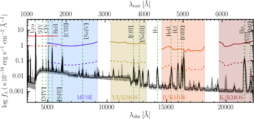
Figure 9.— Predicted median spectra for the models in our grid that satisfy simultaneously SB${}_{\rm Ly\alpha}\sim 7\times 10^{-18}$ erg s^-1 cm^-2 arcsec^-2, He II/Ly$\alpha$ $<0.18$, and C IV/Ly$\alpha$ $<0.16$. The gray shaded area indicates the maximum and the minimum possible value for the selected models at each wavelength, showing the range of all the possible values, including the variation of the EUV slope, i.e. $\alpha_{\rm EUV}=-2.3,-1.7$, and $-1.1$ (see Appendix). Our Keck/LRIS 3$\sigma$ sensitivity limit calculated in 1 arcsec² and over 3000 km s^-1, is plotted as a solid red line, together with the 3$\sigma$ sensitivity of MUSE and KMOS (YJ, H, K gratings) for an exposure time of 10 hours (other colored solid lines). The red dashed line indicates our 3$\sigma$ sensitivity limit average over an aperture of 20 arcsec² (see §3), while all the other dashed lines show the sensitivity averaged over an aperture of 300 arcsec², i.e. $SB_{\rm limit}=SB_{1\sigma}/\sqrt{A}$. The principal emission lines are indicated by the green vertical dashed lines. The lines that may be detectable in the future, given appropriate physical conditions (i.e. $n_{H},Z$) in the targeted nebula are He II, [C III], C IV, [Si III], [O II], [O III], H$\beta$, and H$\alpha$.

For comparison we show our Keck/LRIS 3$\sigma$ sensitivity limits from §2 calculated by averaging over a 1 arcsec² aperture and over a 3000 km s^-1 velocity interval (solid red line), together with the 3$\sigma$ sensitivity limits for 10 hours of integration with the Multi Unit Spectroscopic Explorer (MUSE) (Bacon et al. 2010; solid blue line), and with the K-band Multi Object Spectrograph (KMOS) (Sharples et al. 2006; gold, orange, and dark-red solid lines), on the VLT, computed for the same spatial and spectral aperture. Note that these sensitivity limits can be lowered by assuming a certain amount of spatial averaging, following the relation $SB_{\rm limit}=SB_{1\sigma}/\sqrt{A}$, where $A$ is the area in arcsec² over which the data are averaged. Indeed, we employed this approach in §3, and averaged over an area of 20 arcsec² to obtain a more sensitive constraint on the He II/Ly$\alpha$ and C IV/Ly$\alpha$ line ratios, and this lower SB level is indicated by the red dashed line in Figure 9. In contrast with a longslit, integral-field units like MUSE and KMOS, as well as the upcoming Keck Cosmic Web Imager (KCWI, Morrissey et al. 2012), provide near continuous spatial sampling over wide areas, and are thus the ideal instruments for trying to detect extended line emission from the CGM. Thus for MUSE and KMOS, we have assumed that we can average over an area as large as $300$ arcsec², as shown by the colored dashed lines, and indeed this approach has already been used with the Cosmic Web Imager (Martin et al. 2014a) to study lower SB Ly$\alpha$ emission (Martin et al. 2014b).

Given these expected sensitivities, in Figure 9 we indicate the principal emission lines that may be detectable (vertical green dashed lines), whose observation would provide additional constraints on the properties of the emitting gas. The large range of metallicities in our grid $Z=10^{-3}Z_{\odot}$ to $Z_{\odot}$, results in a correspondingly large range of metal emission line strengths, whereas the Hydrogen Balmer lines and He II are much less sensitive to metallicity and thus show very little variation across our model grid.

Focusing first on the primordial elements, we see that He II is the strongest line, and in particular it is stronger than H$\alpha$. Indeed, if the Helium is completely doubly ionized then He II/H$\alpha\sim 3$, and although it decreases to lower values for lower ionization parameters (higher densities), it always remains higher than unity. As we have argued in §5, a detection of He II can be used to measure the volume density $n_{\rm H}$ of the emitting gas. Further, by comparing the morphology, size, and kinematics of the non-resonant extended He II emission to that of Ly$\alpha$, one can test whether resonant scattering of Ly$\alpha$ plays an important role in the structure of the nebula (Prescott et al. 2015a). Naively, one might have thought that H$\alpha$ would be ideal for this purpose given that it is the strongest Hydrogen recombination line after Ly$\alpha$. However, our models indicate that for photoionization by a hard source, the He II line is always stronger than H$\alpha$, and given that He II is in the optical whereas H$\alpha$ is in the near-IR, it is also much easier to detect.

Figure 9 shows that deep integrations in the near-IR with KMOS will consistently detect the Hydrogen Balmer lines H$\alpha$ and H$\beta$. When compared to the Ly$\alpha$ emission, these lines would allows one to determine the extinction due to dust (Osterbrock & Ferland 2006). Further, at the low densities we consider ($n_{\rm H}\ll 10^{4}$ cm^-3), any departure of the ratios H$\alpha$/H$\beta$ and Ly$\alpha$/H$\beta$ from their case B values provide information on the importance of collisional excitation of Ly$\alpha$, which is exponentially sensitive to the gas temperature (Ferland & Osterbrock 1985). In other words, the amount of collisional excitation is set by the equilibrium temperature of the gas, which is set by the balance of heating and cooling. Photoionization by a hard source will result in a characteristic temperature and hence ratio of Ly$\alpha$/H$\beta$ set by the ionizing continuum slope, whereas an additional source of heat, as has been postulated in gravitational cooling radiation scenarios for Ly$\alpha$ nebulae (e.g. Rosdahl & Blaizot 2012), would increase the amount of collisionally excited Ly$\alpha$ and hence the ratio of Ly$\alpha$/H$\beta$.

Figure 9 shows also that one could probably detect metal emission lines depending on the physical conditions in the gas, which are parameterized by $n_{\rm H}$ and $Z$. In particular, if the gas has metallicity $Z>0.1Z_{\odot}$, a deep integration with MUSE would detect C IV, [C III], and, for metallicity close to solar, also [Si III] $\lambda 1883$. In the near-IR, we see that a deep integration with KMOS would detect [O III] for $Z>0.1Z_{\odot}$, and [O II] for metallicity close to solar. Note that for similar bright nebulae at different redshifts, it would be possible to detect other lines in extended emission for particular $n_{\rm H}$ and $Z$ combinations, e.g. Si IV $\lambda 1394$, and [N IV] $\lambda 1480$.

According to Figure 9, a good observational strategy is thus to look for the He II line, which appears to be the strongest and easiest line to detect, and our analysis in §5 indicates that its detection constrains the gas properties to lie on a line in the $n_{\rm H}$-$Z$ plane (see panel ‘a’ in Figure 7). Following our discussion of C IV (panel ‘b’ of Figure 7), the detection of any metal line would define another line in the $n_{\rm H}$-$Z$ plane, and the intersection of these curves would determine the $n_{\rm H}$ and $Z$ of the gas. These conclusions will be somewhat sensitive to the assumed spectral slope in the UV (see Appendix), but given the different ionization thresholds to ionized Carbon to C IV (47.9eV), and Oxygen to O III (35.1eV) or O II (13.6eV), it is clear that detections or limits on multiple metal lines from high and low ionization states would also constrain the slope $\alpha_{\rm EUV}$ of the ionizing continuum.

To summarize, our photoionization modeling and analysis provide a compelling motivation to find more bright nebulae by surveying large samples of quasars and HzRGs, and conducting NB emission line surveys of LABs over large areas. Armed with the brightest and largest giant nebulae like UM287, one can conduct deep observations with IFUs, and combined with suitable spatial averaging, this will uncover a rich emission line spectrum from the CGM and its interface with the IGM, which can be used to constrain the physical properties of the emitting gas, and shed light on physical mechanism powering giant nebulae.

7. Caveats

In section §5, under the assumption of photoionization by the central QSO, and in the context of a simple model for the gas distribution, we showed how our upper limits on the He II/Ly$\alpha$ and C IV/Ly$\alpha$ ratios, can set constraints on the physical properties of the cool gas observed in emission. However, this simple modeling is just a zeroth-order approximation to a more complicated problem which is beyond the scope of the present work. In what follows we highlight some issues which should be examined further.

Radial Dependence: for simplicity we have evaluated the ionizing flux at a single radial location for input into Cloudy. We have tested the impact of this assumption, by decreasing $R$ from 160 kpc to 100 kpc, and find that our lower limit on the density increases by 0.4 dex. This results from the fact that the He II/Ly$\alpha$ ratio varies with ionization parameter $U$, and our upper limit on the line ratio sets a particular value of $U$. By decreasing $R$, the density $n_{\rm H}$ corresponding to this specific value of $U$ thus increases by a factor $R^{2}$. The variation of the ionizing flux with radius, should be taken into account in a more detailed calculation.

Slope of the Ionizing Continuum: we have assumed $\alpha_{\rm EUV}=-1.7$ (Lusso et al. 2015). However, estimates for $\alpha_{\rm EUV}$ in the literature vary widely (Zheng et al. 1997; Scott et al. 2004; Shull et al. 2012), most likely because of uncertainties introduced when correcting for absorption due to the IGM or because of the heterogeneity of the samples considered. Furthermore, the shape of the ionizing continuum near the He II edge of 4 Rydberg is not well constrained. For detailed analysis on the sensitivity of our results to the ionizing continuum slope, see the Appendix, where we consider two different ionizing slopes, i.e. $\alpha_{\rm EUV}=-1.1$ and $-2.3$. We find that a harder ionizing slope $\alpha_{\rm EUV}=-1.1$ moves our lower limit on the density from $n_{\rm H}\gtrsim 3$ cm^-3 to $n_{\rm H}\gtrsim 1$ cm^-3. Thus, the uncertainty on the ionizing slope has an order unity impact on our constraints of the volume density. As discussed at the end of §6, the detection of additional metal lines with a range of ionization thresholds would further constrain $\alpha_{\rm EUV}$.

Covering Factor: Based on the morphology of the emission we argued $f_{\rm C}\gtrsim 0.5$, but assumed the value of $f_{\rm C}=1.0$ for simplicity. The $f_{\rm C}$ drops out of the line ratios (see eqn. (3) and (8)), however our model depends on $f_{C}$, since we were selecting only models able to reproduce the observed Ly$\alpha$ SB, which varies linearly with covering factor. We estimate that lowering the covering factor to $f_{\rm C}=0.4$, only change our lower limit on the density at the $15\%$ level. As discussed in section §5, lowering $f_{\rm C}$ results in a reduction of the number of models which are able to reproduce the observed Ly$\alpha$ SB, because models with high $n_{\rm H}N_{\rm H}$ valuse become optically thick, and thus over-estimate the Ly$\alpha$ emission. In particular, there are no models which reproduce the observed Ly$\alpha$ SB for low covering factors ($f_{\rm C}<0.3$). Thus our conclusions are largely insensitive to the covering factor we assumed.

Geometry: we have assumed the emitting clouds are spatially uniformly distributed throughout a spherical halo. This simple representation would need geometric corrections to take into account more complicated gas distributions, such as variation of the covering factor with radius or filamentary structures. However, these corrections should be of order unity, and are thus likely sub-dominant compared to other effects.

Single Uniform Cloud Population: our simple model assumes a single population of clouds which all have the same constant physical parameters $N_{\rm H}$, $n_{\rm H}$, and $Z$, following a uniform spatial distribution throughout the halo. In reality one expects a distribution of cloud properties, and a radial dependence. Indeed, Binette et al. (1996) argued that a single population of clouds is not able to simultaneously explain both the high and low ionization lines in the extended emission line regions of HzRGs, and instead invoked a mixed population of completely ionized clouds and partially ionized clouds. While for the case of extended emission line regions (EELRs) around quasars, which are on smaller scale $R<50\,{\rm kpc}$ than studied here, detailed photoionization modeling of spectroscopic data has demonstrated that at least two density phases are likely required: a diffuse abundant cloud population with $n_{\rm H}\sim 1$ cm^-3, and much rarer dense clouds with $n_{\rm H}\sim 500$ cm^-3 (Stockton et al. 2002; Fu & Stockton 2007; Hennawi et al. 2009). Further, these clouds may be in pressure equilibrium with the ionizing radiation (Dopita et al. 2002, Stern et al. 2014), as has been invoked in modeling the narrow-line regions of AGN. Future detailed modeling of multiple emission lines from giant nebulae, analogous to previous work on the smaller scale of EELRs (Stockton et al. 2002; Fu & Stockton 2007), might provide information on multiple density phases.

In order to properly address the aforementioned issues, the ideal approach would be to conduct a full radiative transfer calculation on a three dimensional gas distribution, possibly taken from a cosmological hydrodynamical simulation. Cantalupo et al. (2014) carried out exactly this kind of calculation treating both ionizing and resonant radiative transfer, however this analysis was restricted only to the Ly$\alpha$ line. Full radiative transfer coupled to detailed photoionization modeling as executed by Cloudy would clearly be too computationally challenging. However it would be interesting to introduce the solutions of 1-D Cloudy slab models into a realistic gas distribution drawn from a cosmological simulation. This would be relatively straightforward for the case of optically thin nebulae (e.g. van de Voort & Schaye 2013).

8. Summary and Conclusions

To study the kinematics of the extended Ly$\alpha$ line and to search for extended He II $\lambda 1640$ and C IV $\lambda 1549$ emission, we obtained deep spectroscopy of the UM287 nebula (Cantalupo et al. 2014) with the Keck/LRIS spectrograph. Our spectrum of the nebula provides evidence for large motions suggested by the Ly$\alpha$ line of FWHM${}_{\rm gauss}\sim 500$ km s^-1 which are spatially coherent on scales of $\sim$150 kpc. There is no evidence for a “double-peaked” line along either of the slits, as might be expected in a scenario where resonant scattering determines the Ly$\alpha$ kinematic structure.

Although our observations achieve an unprecedented sensitivity in the He II and C IV line (${\rm SB}_{3\sigma}\simeq 10^{-18}$ erg s^-1 cm^-2 arcsec^-2, average over 1″ $\times$ 20″and $\Delta v=3000$ km s^-1) for giant Ly$\alpha$ nebulae, we do not detect extended emission in either line for both of our slit orientations. We constrain the He II/Ly$\alpha$ and C IV/Ly$\alpha$ ratios to be $<0.18$ (3$\sigma$), and $<0.16$ (3$\sigma$), respectively.

To interpret these non-detections, we constructed models of the emission line ratios, assuming photoionization by the central quasar and a simple spatial distribution of cool gas in the quasar halo. We find that:

• if the gas clouds emitting Ly$\alpha$ are optically thick to ionizing radiation, then the nebula would be $\sim$$120\times$ brighter than observed, unless we assume an unrealistically low covering factor, i.e. $f_{C}\lesssim 0.02$, which is in conflict with the smooth morphology of the nebula. Thus we conclude that the covering factor of cool gas clouds in the nebula is high $f_{\rm C}\gtrsim 0.5$, and that the gas in the nebula is highly ionized, resulting in gas clouds optically thin ($N_{\rm HI}<17.2$) to ionizing radiation.

• The He II line is a recombination line and thus, once the density is fixed, its emission depends primarily on the fraction of Helium that is doubly ionized. On the other hand, the C IV emission line is an important coolant and is powered primarily by collisional excitation, and thus its emission depends on the amount of Carbon in the C⁺³ ionic state. As we know the ionizing luminosity of the central quasar, and the Ly$\alpha$ SB of the nebula, constraints on the He II/Ly$\alpha$ and C IV/Ly$\alpha$ ratios determine where the gas lives in the $n_{\rm H}-Z$ diagram.

• Photoionization from the central quasar is consistent with the Ly$\alpha$ emission and the He II and C IV upper limits, provided that the gas distribution satisfies the following constraints:

  1. $n_{\rm H}\gtrsim 3$ cm^-3,

  2. $N_{\rm H}\lesssim 10^{20}$ cm^-2,

  3. $R\lesssim 20$ pc.

  If these properties hold through the entire nebula, it then follows that the total cool gas ($T\sim 10^{4}$ K) mass is $M_{\rm c}\lesssim 6.4\times 10^{10}$ M_⊙.

Because the Ly$\alpha$ surface brightness scales as SB${}_{\rm Ly\alpha}\propto n_{\rm H}N_{\rm H}$, whereas the total cool gas mass as $M_{\rm c}\propto N_{\rm H}$, observations of Ly$\alpha$ emission cannot independently determine the cool gas mass and $n_{\rm H}$ (or the gas clumping factor $C$), which limited the previous modeling by Cantalupo et al. (2014). Our non-detection of He II/Ly$\alpha$ combined with photoionization modeling allows us to break this degeneracy, and independently constrain both $n_{\rm H}$ and $M_{\rm c}$.

Our results point to the presence of a population of compact ($R\lesssim 20$ pc) cool gas clouds in the CGM at ISM-like densities of $n_{\rm H}\gtrsim 3\,{\rm cm}^{-3}$ moving through the quasar halo at velocities $\simeq 500\,{\rm km\,s^{-1}}$. It is well known that even by $z\sim 2$, the gas in the massive $M\sim 10^{12.5}$ M_⊙ halos hosting quasars is expected to be dominated by a hot shock-heated plasma at the virial temperature $T\sim 10^{7}\,{\rm K}$. Cool clouds moving rapidly through a hot plasma will be disrupted by hydrodynamic instabilities on the cloud-crushing timescale (e.g. Jones et al. 1994; Schaye et al. 2007; Agertz et al. 2007; Crighton et al. 2015; Scannapieco & Brüggen 2015)

$$t_{\rm cc} \approx 1.3\,{\rm Myr}\left(\frac{R}{20\,{\rm pc}}\right)\left(\frac{v}{500\,{\rm km\,s^{-1}}}\right)^{-1}$$ (10)

$$\times \left(\frac{n_{\rm cl}/n_{\rm halo}}{1000}\right)^{1/2},$$

where we assume that the Ly$\alpha$ line trace the kinematics of the cool clouds, and that the cloud-halo density contrast is of the order of 1000 ($n_{\rm halo}\sim 10^{-3}$ cm^-3). If there is hot plasma present in the halo, these clouds are thus very short lived, and can only be transported $\sim 0.7\,{\rm kpc}$ before being disrupted. These very short disruption timescales thus require a mechanism that makes the clumps resistant to hydrodynamic instabilities, such as confinement by magnetic fields (e.g. McClure-Griffiths et al. 2010; McCourt et al. 2015), otherwise the population of cool dense clouds must be constantly replenished. In the latter scenario, the short lived clouds might be formed in situ, via cooling and fragmentation instabilities. If the hot plasma pressure confines the clouds, this might compresses them to high enough densities (Fall & Rees 1985; Maller & Bullock 2004; Mo & Miralda-Escude 1996) to explain our results. Emission line nebulae from cool dense gas has also been observed at the centers of present-day cooling flow clusters (Heckman et al. 1989; McDonald et al. 2010), albeit on much smaller scales $\lesssim 50\,{\rm kpc}$. The giant Ly$\alpha$ nebula in UM287 might be a manifestation of the same phenomenon, but with much larger sizes and luminosities, reflecting different physical conditions at high-redshift. Detailed study of the hydrodynamics of cool dense gas clouds, with properties consistent with our constraints, moving through hot plasma are clearly required (Scannapieco & Brüggen 2015).

As we showed in §6, deep observations ($\sim 10\,{\rm hr}$) of UM287 and other giant nebulae with the new integral field units such as MUSE (Bacon et al. 2010), KCWI (Morrissey et al. 2012), and KMOS (Sharples et al. 2006), combined with spatial averaging, will be able to detect extended emission from other lines besides Ly$\alpha$ (see Figure 9). In particular, the strongest line will be He II which should be routinely detectable, and following our analysis, will enable measurements of the volume density $n_{\rm H}$ of the gas. Specifically, a 10 hour MUSE integration would correspond to a sensitivity in He II/Ly$\alpha$ of $\sim$0.01 ($3\sigma$ in 300 arcsec² ), which would allow us to probe gas densities as high as $n_{\rm H}=1000$ cm^-3. Although we have argued that the UM287 is powered by photoionization, which is compelling given the presence of a hyper-luminous quasar, a non-detection of He II in a 10hr MUSE integration would imply such extreme gas densities in the CGM, i.e. $n_{\rm H}>1000$ cm^-3, that one might need to reconsider other potential physical mechanisms for powering the Ly$\alpha$ nebula which do not produce He II, such as cold-accretion (e.g., Haiman et al. 2000; Furlanetto et al. 2005; Dijkstra et al. 2006a; Faucher-Giguère et al. 2010; Rosdahl & Blaizot 2012), star-formation (e.g., Cen & Zheng 2013), or superwinds (e.g., Taniguchi & Shioya 2000; Taniguchi et al. 2001; Wilman et al. 2005). Furthermore, comparison of the morphology and kinematics of the nebula in He II and Ly$\alpha$ can be used to test whether resonant scattering of Ly$\alpha$ photons is important. Although H$\alpha$ could also be used to test the impact of resonant scattering, it is always fainter than He II and redshifted into the near-IR, where a detection of extended emission is much more challenging.

In a photoionization scenario, a 10 hr observation of UM287 or a comparable nebula with MUSE (or KCWI) and KMOS would result in a rich emission line spectrum of the CGM, which, depending on the properties of the gas (i.e. $n_{\rm H}$ and $Z$), could yield detections of Ly$\alpha$, [N IV], Si IV, [Ne IV], C IV, [C III], [Si III], [O III], [O II], H$\beta$, and H$\alpha$. This would enable modeling of the CGM at a comparable level of detail as models of H II regions and the narrow and broad-line regions of AGN, resulting in comparably detailed constraints on the physical properties of the gas.

Current estimates suggest that $\sim 10-20\%$ of quasars exhibit bright giant nebulae (Hennawi et al., 2015) like UM287, and our results provide a compelling motivation to expand current samples by surveying large numbers of quasars with instruments like MUSE and KCWI. At the same time, this same survey data would enable one to compute a stacked composite CGM spectrum of quasars which do not exhibit bright nebulae, constraining the gas properties around typical quasars.

Appendix A Effects of a Variation of the EUV Slope of the Input Spectrum

We test the robustness of our results to the change of the slope of the EUV as mentioned in Section §4.3. In particular, we model the extremes of the range allowed by the recent estimates of Lusso et al. (2015), i.e. $\alpha_{\rm EUV}=-1.7\pm 0.6$. To fulfill the $\alpha_{\rm OX}$ requirement of Strateva et al. (2005) as explained in Section §4.3, the value $\alpha_{\rm EUV}=-2.3$ and -1.1 imply at higher energies ($30\,{\rm Ryd}<h\nu<2{\rm keV}$) a slope $\alpha=-0.36$ and -2.93, respectively. In our fiducial input spectrum ($\alpha_{\rm EUV}=-1.7$), the photoionization rate at the Lyman limit is

$$\Gamma=\frac{1}{4\pi r^{2}}\int_{\nu_{\rm LL}}^{\infty}\frac{L_{\nu}}{h\nu}\sigma_{\nu}d\nu=6.7\times 10^{-9}\,{\rm s^{-1}},$$ (A1)

while at 4 Ryd, i.e. at the ionization energy of He II, the photoionization rate is $\Gamma_{\rm 4Ryd}\sim 1.0\times 10^{-11}$ s^-1. By changing the slope in the extreme ultraviolet from $\alpha_{\rm EUV}=-1.7$, to -1.1 and to -2.3, we increase the photoionization rate by $\sim$15% and decrease it by $\sim$13%, respectively. Instead, for the same change, the $\Gamma_{\rm 4Ryd}$ is increased/decreased by a factor of 2.6, respectively. As it is clear from the small changes in $\Gamma$, the Hydrogen ionization state is not affected by the change in slope, and the models are always optically thin. Conversely, as expected, the changes in $\Gamma_{\rm 4Ryd}$ affect He II and C IV. The general trend is that a softer slope, e.g. $\alpha_{\rm EUV}=-2.3$, produces fewer He II ionizing photons, and thus at fixed density the He III fraction will be lower, resulting in lower He II recombination emission. This thus leads to a lower He II/Ly$\alpha$ ratio. Similarly, a softer slope is less effective in ionizing Carbon. In particular, at fixed ionization parameter $U$, the amount of Carbon in the C⁺³ phase is lower for a softer slope.

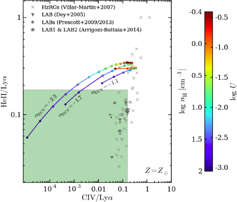
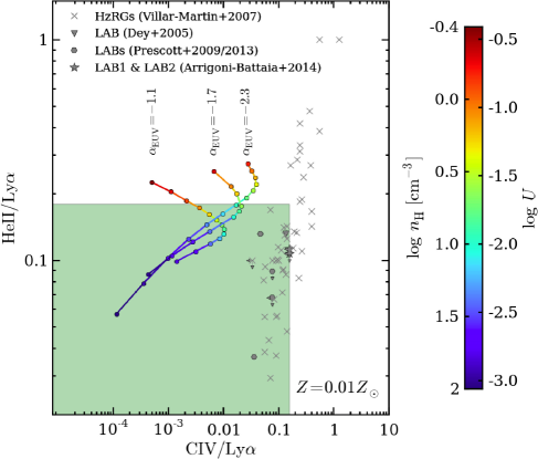
Figure 10.— HeII/Ly$\alpha$ versus CIV/Ly$\alpha$ log-log plot. Our upper limits on the HeII/Ly$\alpha$ and CIV/Ly$\alpha$ ratios are compared with the Cloudy photoionization models that reproduce the observed SB${}_{\rm Ly\alpha}\sim 7\times 10^{-18}$ erg s^-1 cm^-2 arcsec^-2. Upper panel: comparison of the model grids for different EUV slopes ($\alpha_{\rm EUV}=-1.1,-1.7,-2.3$) at $Z=Z_{\odot}$. A harder $\alpha_{\rm EUV}$ completely doubly ionize Helium at higher density. Bottom panel: same as the upper panel, but at $Z=0.01Z_{\odot}$. In this case, the Ly$\alpha$ line is also powered by collisions, reshaping the trajectories (see text for explanation on the trends in this Figure). In both panels, the models are color coded following the ionization parameter $U$, or equivalently the volume density $n_{\rm H}$ (see color bar on the right). The green shaded area represents the region defined by the upper limits of the UM287 nebula. See Figure 11 for a better visualization of the constraints on the physical parameters.

In Figure 10 we compare our grids of models with different EUV slopes at two different metallicities, i.e. $Z=Z_{\odot}$, and $0.01Z_{\odot}$, in the He II/Ly$\alpha$ versus C IV/Ly$\alpha$ plot. The dependencies outlined above, are better visible in the plot for solar metallicity (upper panel) because the Ly$\alpha$ line is mainly produced by recombinations and its behavior is not influencing the general trends. From the figure, it is clear that a grid with a softer slope (see grid with $\alpha_{\rm EUV}=-2.3$) can reach lower He II/Ly$\alpha$ ratios because the fraction of doubly ionized Helium is lower at high densities. In the same upper panel of Figure 10 it is also evident that the simulation grids for different UV slopes all asymptote to a fixed He II/Ly$\alpha$ ratio when Helium is completely doubly ionized, which occurs at slightly different $n_{\rm H}$ (or equivalently $U$) for each slope. Note that the value of the asymptotic He II/Ly$\alpha$ ratio varies slightly with slope. Indeed, as mentioned in section §5, since this asymptotic value is proportional to the ratio of the recombination coefficients of He II and Ly$\alpha$, the value depends on temperature (eqn. (5)). Higher temperatures, which arise for a harder slope, lead to a lower asymptotic He II/Ly$\alpha$ ratio.

In the bottom panel of Figure 10, we show the same comparison at $Z=0.01Z_{\odot}$. In this case the trends are masked by the Ly$\alpha$ line, which is powered also by collisions. Indeed, the saturation in the He II/Ly$\alpha$ ratio is not appreciable because, given the dependence on density of the collisional contribution to the Ly$\alpha$ line, the ratio is progressively lowered at higher density. However, it is still appreciable that the C IV/Ly$\alpha$ ratio is moved to lower ratios for higher slopes above log$U\sim-1.5$. This is mainly due to the fact that Carbon goes to higher ionization state, lowering the fraction of Carbon in the C⁺³ species. Thus, in our case study, where the input spectrum is not well known, the dependence of the amount of C⁺³ on the slope of the EUV makes the C IV line a weak metallicity indicator.

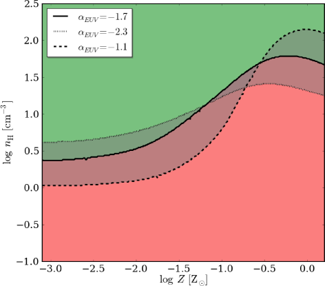
Figure 11.— Schematic representation on how a variation in $\alpha_{\rm EUV}$ affects the constraints in $n_{\rm H}$ and $Z$. The green area highlights the region of the parameter space selected by the upper limit He II/Ly$\alpha$ $<0.18$ (see panel ‘a’ of Figure 7). The solid, dashed, and dotted lines show the location of this upper limit for $\alpha_{\rm EUV}=-1.7,-1.1$ , and $-2.3$, respectively. It is evident that a change in the ionizing slope do not affect our main conclusions. Namely, if the nebula is photoionized by the UM287 quasar, there should be a population of dense cool gas clumps with very small sizes ($\lesssim$tens of pc).

Changes in the slope $\alpha_{\rm EUV}$ only slightly modifies the constraints on $n_{\rm H}$ that we previously obtained. In particular, since the He II/Ly$\alpha$ ratio gives the stronger constraints, in Figure 11 we show how a variation in the EUV slope affects the selection of $n_{\rm H}$ (compare Figure 10 and 11). This Figure highlights in green the parameter space favored by our upper limits (the lines show the location of the upper limit He II/Ly$\alpha$ $=0.18$). The mild change in the location of the line is explained by the dependencies outlined above. At a fixed low metallicity, where the Ly$\alpha$ line is an important coolant, i.e. log$Z<-1.5Z_{\odot}$, a harder slope moves the lower limit boundary implied by our measurement on the He II/Ly$\alpha$ ratio to lower densities. Indeed, the expected increase of the He II line due to a harder slope is washed out by the increase in the emission in the Ly$\alpha$ line due to collisions. Thus, our constraint on the density that we quote in the main text is weakened from $n_{\rm H}\gtrsim 3$ cm^-3 to $n_{\rm H}\gtrsim 1$ cm^-3. On the other hand, at higher metallicities, a harder UV slope will doubly ionize Helium at higher density, moving the lower limit boundary implied by our measurement to higher densities. For example, at solar metallicity, the limit is moved to $\gtrsim 100$ cm^-3 from $\gtrsim 40$ cm^-3.

Thus, in conclusion, our ignorance on the slope of the EUV has a small effect on our density constraints and makes the C IV line a weak metallicity indicator. However, as discussed at the end of §6, the detection of multiple metal lines with a range of ionization energies would indirectly constrain $\alpha_{\rm EUV}$, and simultaneously constrain the metallicity of the gas.

References

- Agertz et al. (2007) Agertz, O., Moore, B., Stadel, J., et al. 2007, MNRAS, 380, 963
- Alam & Miralda-Escudé (2002) Alam, S. M. K., & Miralda-Escudé, J. 2002, ApJ, 568, 576
- Arrigoni Battaia et al. (2015) Arrigoni Battaia, F., Hennawi, J., Prochaska, J., & Cantalupo, S. 2015, in prep.
- Arrigoni Battaia et al. (2014a) Arrigoni Battaia, F., Hennawi, J. F., Cantalupo, S., & Prochaska, J. X. 2014a, Proc. IAU Symp. #304: Multiwavelength AGN Surveys and Studies, Cambridge Univ. Press, 253
- Arrigoni Battaia et al. (2014b) Arrigoni Battaia, F., Yang, Y., Hennawi, J. F., et al. 2014b, ArXiv e-prints, arXiv:1407.2944
- Bacon et al. (2010) Bacon, R., Accardo, M., Adjali, L., et al. 2010, in Society of Photo-Optical Instrumentation Engineers (SPIE) Conference Series, Vol. 7735, Society of Photo-Optical Instrumentation Engineers (SPIE) Conference Series
- Baskin et al. (2014) Baskin, A., Laor, A., & Stern, J. 2014, MNRAS, 438, 604
- Ben Bekhti et al. (2009) Ben Bekhti, N., Richter, P., Winkel, B., Kenn, F., & Westmeier, T. 2009, A&A, 503, 483
- Bergeron et al. (2004) Bergeron, J., Petitjean, P., Aracil, B., et al. 2004, The Messenger, 118, 40
- Binette et al. (1993) Binette, L., Wang, J. C. L., Zuo, L., & Magris, C. G. 1993, AJ, 105, 797
- Binette et al. (1996) Binette, L., Wilson, A. S., & Storchi-Bergmann, T. 1996, A&A, 312, 365
- Boesgaard & Steigman (1985) Boesgaard, A. M., & Steigman, G. 1985, ARA&A, 23, 319
- Cantalupo et al. (2014) Cantalupo, S., Arrigoni-Battaia, F., Prochaska, J. X., Hennawi, J. F., & Madau, P. 2014, Nature, 506, 63
- Cantalupo et al. (2012) Cantalupo, S., Lilly, S. J., & Haehnelt, M. G. 2012, MNRAS, 425, 1992
- Cantalupo et al. (2007) Cantalupo, S., Lilly, S. J., & Porciani, C. 2007, ApJ, 657, 135
- Cantalupo et al. (2005) Cantalupo, S., Porciani, C., Lilly, S. J., & Miniati, F. 2005, ApJ, 628, 61
- Cen & Zheng (2013) Cen, R., & Zheng, Z. 2013, ApJ, 775, 112
- Charlot & Fall (1993) Charlot, S., & Fall, S. M. 1993, ApJ, 415, 580
- Christensen et al. (2006) Christensen, L., Jahnke, K., Wisotzki, L., & Sánchez, S. F. 2006, A&A, 459, 717
- Crighton et al. (2015) Crighton, N. H. M., Hennawi, J. F., Simcoe, R. A., et al. 2015, MNRAS, 446, 18
- Croft et al. (2002) Croft, R. A. C., Weinberg, D. H., Bolte, M., et al. 2002, ApJ, 581, 20
- Dere et al. (1997) Dere, K. P., Landi, E., Mason, H. E., Monsignori Fossi, B. C., & Young, P. R. 1997, A&AS, 125, 149
- Dey et al. (2005) Dey, A., Bian, C., Soifer, B. T., et al. 2005, ApJ, 629, 654
- Dijkstra et al. (2006a) Dijkstra, M., Haiman, Z., & Spaans, M. 2006a, ApJ, 649, 14
- Dijkstra et al. (2006b) —. 2006b, ApJ, 649, 37
- Dijkstra & Loeb (2008) Dijkstra, M., & Loeb, A. 2008, MNRAS, 386, 492
- Dopita et al. (2002) Dopita, M. A., Groves, B. A., Sutherland, R. S., Binette, L., & Cecil, G. 2002, ApJ, 572, 753
- Fall & Rees (1985) Fall, S. M., & Rees, M. J. 1985, ApJ, 298, 18
- Fardal et al. (2001) Fardal, M. A., Katz, N., Gardner, J. P., et al. 2001, ApJ, 562, 605
- Farina et al. (2013) Farina, E. P., Falomo, R., Decarli, R., Treves, A., & Kotilainen, J. K. 2013, MNRAS, 429, 1267
- Faucher-Giguere et al. (2014) Faucher-Giguere, C.-A., Hopkins, P. F., Keres, D., et al. 2014, ArXiv e-prints, arXiv:1409.1919
- Faucher-Giguère et al. (2010) Faucher-Giguère, C.-A., Kereš, D., Dijkstra, M., Hernquist, L., & Zaldarriaga, M. 2010, ApJ, 725, 633
- Ferland & Osterbrock (1985) Ferland, G. J., & Osterbrock, D. E. 1985, ApJ, 289, 105
- Ferland et al. (2013) Ferland, G. J., Porter, R. L., van Hoof, P. A. M., et al. 2013, Rev. Mexicana Astron. Astrofis., 49, 137
- Francis & Bland-Hawthorn (2004) Francis, P. J., & Bland-Hawthorn, J. 2004, MNRAS, 353, 301
- Fu & Stockton (2007) Fu, H., & Stockton, A. 2007, ApJ, 666, 794
- Fumagalli et al. (2014) Fumagalli, M., Hennawi, J. F., Prochaska, J. X., et al. 2014, ApJ, 780, 74
- Furlanetto et al. (2005) Furlanetto, S. R., Schaye, J., Springel, V., & Hernquist, L. 2005, ApJ, 622, 7
- Fynbo et al. (1999) Fynbo, J. U., Møller, P., & Warren, S. J. 1999, MNRAS, 305, 849
- Geach et al. (2007) Geach, J. E., Smail, I., Chapman, S. C., et al. 2007, ApJ, 655, L9
- Geach et al. (2009) Geach, J. E., Alexander, D. M., Lehmer, B. D., et al. 2009, ApJ, 700, 1
- Gould & Weinberg (1996) Gould, A., & Weinberg, D. H. 1996, ApJ, 468, 462
- Greene et al. (2011) Greene, J. E., Zakamska, N. L., Ho, L. C., & Barth, A. J. 2011, ApJ, 732, 9
- Groves et al. (2004) Groves, B. A., Dopita, M. A., & Sutherland, R. S. 2004, ApJS, 153, 75
- Haiman & Rees (2001) Haiman, Z., & Rees, M. J. 2001, ApJ, 556, 87
- Haiman et al. (2000) Haiman, Z., Spaans, M., & Quataert, E. 2000, ApJ, 537, L5
- Hayes et al. (2011) Hayes, M., Scarlata, C., & Siana, B. 2011, Nature, 476, 304
- Heckman et al. (1989) Heckman, T. M., Baum, S. A., van Breugel, W. J. M., & McCarthy, P. 1989, ApJ, 338, 48
- Heckman et al. (1991a) Heckman, T. M., Lehnert, M. D., Miley, G. K., & van Breugel, W. 1991a, ApJ, 381, 373
- Heckman et al. (1991b) Heckman, T. M., Miley, G. K., Lehnert, M. D., & van Breugel, W. 1991b, ApJ, 370, 78
- Hennawi et al. (2015) Hennawi, J., Prochaska, J., Cantalupo, S., & Arrigoni Battaia, F. 2015, submitted to Science
- Hennawi & Prochaska (2007) Hennawi, J. F., & Prochaska, J. X. 2007, ApJ, 655, 735
- Hennawi & Prochaska (2013) —. 2013, ApJ, 766, 58
- Hennawi et al. (2009) Hennawi, J. F., Prochaska, J. X., Kollmeier, J., & Zheng, Z. 2009, ApJ, 693, L49
- Hennawi et al. (2006) Hennawi, J. F., Prochaska, J. X., Burles, S., et al. 2006, ApJ, 651, 61
- Hogan & Weymann (1987) Hogan, C. J., & Weymann, R. J. 1987, MNRAS, 225, 1P
- Hu & Cowie (1987) Hu, E. M., & Cowie, L. L. 1987, ApJ, 317, L7
- Humphrey et al. (2006) Humphrey, A., Villar-Martín, M., Fosbury, R., Vernet, J., & di Serego Alighieri, S. 2006, MNRAS, 369, 1103
- Humphrey et al. (2008) Humphrey, A., Villar-Martín, M., Vernet, J., et al. 2008, MNRAS, 383, 11
- Husemann et al. (2013) Husemann, B., Wisotzki, L., Sánchez, S. F., & Jahnke, K. 2013, A&A, 549, A43
- Iocco et al. (2009) Iocco, F., Mangano, G., Miele, G., Pisanti, O., & Serpico, P. D. 2009, Phys. Rep., 472, 1
- Izotov et al. (1999) Izotov, Y. I., Chaffee, F. H., Foltz, C. B., et al. 1999, ApJ, 527, 757
- Jones et al. (1994) Jones, T. W., Kang, H., & Tregillis, I. L. 1994, ApJ, 432, 194
- Landi et al. (2013) Landi, E., Young, P. R., Dere, K. P., Del Zanna, G., & Mason, H. E. 2013, ApJ, 763, 86
- Lau et al. (2015) Lau, M., Prochaska, J., & Hennawi, J. 2015, submitted to ApJ
- Lee et al. (2014) Lee, K.-G., Hennawi, J. F., White, M., et al. 2014, in American Astronomical Society Meeting Abstracts, Vol. 223, American Astronomical Society Meeting Abstracts, 457.11
- Lusso et al. (2015) Lusso, E., Worseck, G., Hennawi, J. F., et al. 2015, ArXiv e-prints, arXiv:1503.02075
- Maller & Bullock (2004) Maller, A. H., & Bullock, J. S. 2004, MNRAS, 355, 694
- Martin et al. (2014a) Martin, D. C., Chang, D., Matuszewski, M., et al. 2014a, ApJ, 786, 106
- Martin et al. (2014b) —. 2014b, ApJ, 786, 107
- Matsuda et al. (2004) Matsuda, Y., Yamada, T., Hayashino, T., et al. 2004, AJ, 128, 569
- McCarthy (1993) McCarthy, P. J. 1993, ARA&A, 31, 639
- McClure-Griffiths et al. (2010) McClure-Griffiths, N. M., Madsen, G. J., Gaensler, B. M., McConnell, D., & Schnitzeler, D. H. F. M. 2010, ApJ, 725, 275
- McCourt et al. (2015) McCourt, M., O’Leary, R. M., Madigan, A.-M., & Quataert, E. 2015, MNRAS, 449, 2
- McDonald et al. (2010) McDonald, M., Veilleux, S., Rupke, D. S. N., & Mushotzky, R. 2010, ApJ, 721, 1262
- McIntosh et al. (1999) McIntosh, D. H., Rieke, M. J., Rix, H.-W., Foltz, C. B., & Weymann, R. J. 1999, ApJ, 514, 40
- Miley & De Breuck (2008) Miley, G., & De Breuck, C. 2008, A&A Rev., 15, 67
- Mo & Miralda-Escude (1996) Mo, H. J., & Miralda-Escude, J. 1996, ApJ, 469, 589
- Morrissey et al. (2012) Morrissey, P., Matuszewski, M., Martin, C., et al. 2012, in Society of Photo-Optical Instrumentation Engineers (SPIE) Conference Series, Vol. 8446, Society of Photo-Optical Instrumentation Engineers (SPIE) Conference Series, 13
- Nelson et al. (2015) Nelson, D., Genel, S., Pillepich, A., et al. 2015, ArXiv e-prints, arXiv:1503.02665
- Neufeld (1990) Neufeld, D. A. 1990, ApJ, 350, 216
- North et al. (2012) North, P. L., Courbin, F., Eigenbrod, A., & Chelouche, D. 2012, A&A, 542, A91
- Oke (1974) Oke, J. B. 1974, ApJS, 27, 21
- Oke et al. (1995) Oke, J. B., Cohen, J. G., Carr, M., et al. 1995, PASP, 107, 375
- Osterbrock & Ferland (2006) Osterbrock, D. E., & Ferland, G. J. 2006, Astrophysics of Gaseous Nebulae and Active Galactic Nuclei (2nd ed.: Sausalito, CA: Univ. Science Books)
- Overzier et al. (2013) Overzier, R. A., Nesvadba, N. P. H., Dijkstra, M., et al. 2013, ApJ, 771, 89
- Planck Collaboration et al. (2014) Planck Collaboration, Ade, P. A. R., Aghanim, N., et al. 2014, A&A, 571, A16
- Prescott et al. (2009) Prescott, M. K. M., Dey, A., & Jannuzi, B. T. 2009, ApJ, 702, 554
- Prescott et al. (2013) —. 2013, ApJ, 762, 38
- Prescott et al. (2015a) Prescott, M. K. M., Martin, C. L., & Dey, A. 2015a, ApJ, 799, 62
- Prescott et al. (2015b) Prescott, M. K. M., Momcheva, I., Brammer, G. B., Fynbo, J. P. U., & Møller, P. 2015b, ArXiv e-prints, arXiv:1501.05312
- Prochaska & Hennawi (2009) Prochaska, J. X., & Hennawi, J. F. 2009, ApJ, 690, 1558
- Prochaska et al. (2013a) Prochaska, J. X., Hennawi, J. F., & Simcoe, R. A. 2013a, ApJ, 762, L19
- Prochaska et al. (2014) Prochaska, J. X., Wingyee Lau, M., & Hennawi, J. F. 2014, ApJ, 796, 140
- Prochaska et al. (2013b) Prochaska, J. X., Hennawi, J. F., Lee, K.-G., et al. 2013b, ApJ, 776, 136
- Rauch et al. (1999) Rauch, M., Sargent, W. L. W., & Barlow, T. A. 1999, ApJ, 515, 500
- Rauch et al. (2008) Rauch, M., Haehnelt, M., Bunker, A., et al. 2008, ApJ, 681, 856
- Rees (1988) Rees, M. J. 1988, MNRAS, 231, 91P
- Reuland et al. (2003) Reuland, M., van Breugel, W., Röttgering, H., et al. 2003, ApJ, 592, 755
- Reuland et al. (2007) Reuland, M., van Breugel, W., de Vries, W., et al. 2007, AJ, 133, 2607
- Richards et al. (2006) Richards, G. T., Lacy, M., Storrie-Lombardi, L. J., et al. 2006, ApJS, 166, 470
- Rosdahl & Blaizot (2012) Rosdahl, J., & Blaizot, J. 2012, MNRAS, 423, 344
- Rudie et al. (2012) Rudie, G. C., Steidel, C. C., Trainor, R. F., et al. 2012, ApJ, 750, 67
- Scannapieco & Brüggen (2015) Scannapieco, E., & Brüggen, M. 2015, ArXiv e-prints, arXiv:1503.06800
- Schaye et al. (2003) Schaye, J., Aguirre, A., Kim, T.-S., et al. 2003, ApJ, 596, 768
- Schaye et al. (2007) Schaye, J., Carswell, R. F., & Kim, T.-S. 2007, MNRAS, 379, 1169
- Scott et al. (2004) Scott, J. E., Kriss, G. A., Brotherton, M., et al. 2004, ApJ, 615, 135
- Sharples et al. (2006) Sharples, R., Bender, R., Bennett, R., et al. 2006, New A Rev., 50, 370
- Shull et al. (2012) Shull, J. M., Stevans, M., & Danforth, C. W. 2012, ApJ, 752, 162
- Simcoe et al. (2006) Simcoe, R. A., Sargent, W. L. W., Rauch, M., & Becker, G. 2006, ApJ, 637, 648
- Smith & Jarvis (2007) Smith, D. J. B., & Jarvis, M. J. 2007, MNRAS, 378, L49
- Steidel et al. (2000) Steidel, C. C., Adelberger, K. L., Shapley, A. E., et al. 2000, ApJ, 532, 170
- Steidel et al. (2011) Steidel, C. C., Bogosavljević, M., Shapley, A. E., et al. 2011, ApJ, 736, 160
- Stern et al. (2014) Stern, J., Laor, A., & Baskin, A. 2014, MNRAS, 438, 901
- Stockton et al. (2006) Stockton, A., Fu, H., & Canalizo, G. 2006, New A Rev., 50, 694
- Stockton et al. (2002) Stockton, A., MacKenty, J. W., Hu, E. M., & Kim, T.-S. 2002, ApJ, 572, 735
- Strateva et al. (2005) Strateva, I. V., Brandt, W. N., Schneider, D. P., Vanden Berk, D. G., & Vignali, C. 2005, AJ, 130, 387
- Taniguchi & Shioya (2000) Taniguchi, Y., & Shioya, Y. 2000, ApJ, 532, L13
- Taniguchi et al. (2001) Taniguchi, Y., Shioya, Y., & Kakazu, Y. 2001, ApJ, 562, L15
- van de Voort & Schaye (2013) van de Voort, F., & Schaye, J. 2013, MNRAS, 430, 2688
- van Ojik et al. (1997) van Ojik, R., Roettgering, H. J. A., Miley, G. K., & Hunstead, R. W. 1997, A&A, 317, 358
- Vanden Berk et al. (2001) Vanden Berk, D. E., Richards, G. T., Bauer, A., et al. 2001, AJ, 122, 549
- Verhamme et al. (2006) Verhamme, A., Schaerer, D., & Maselli, A. 2006, A&A, 460, 397
- Villar-Martín et al. (2007) Villar-Martín, M., Humphrey, A., De Breuck, C., et al. 2007, MNRAS, 375, 1299
- Villar-Martín et al. (2003a) Villar-Martín, M., Vernet, J., di Serego Alighieri, S., et al. 2003a, MNRAS, 346, 273
- Villar-Martín et al. (2003b) —. 2003b, New A Rev., 47, 291
- Werk et al. (2014) Werk, J. K., Prochaska, J. X., Tumlinson, J., et al. 2014, ApJ, 792, 8
- White et al. (2012) White, M., Myers, A. D., Ross, N. P., et al. 2012, MNRAS, 424, 933
- Wilman et al. (2005) Wilman, R. J., Gerssen, J., Bower, R. G., et al. 2005, Nature, 436, 227
- Yang et al. (2014) Yang, Y., Zabludoff, A., Jahnke, K., & Davé, R. 2014, ArXiv e-prints, arXiv:1407.6801
- Yang et al. (2011) Yang, Y., Zabludoff, A., Jahnke, K., et al. 2011, ApJ, 735, 87
- Yang et al. (2006) Yang, Y., Zabludoff, A. I., Davé, R., et al. 2006, ApJ, 640, 539
- Yang et al. (2012) Yang, Y., Decarli, R., Dannerbauer, H., et al. 2012, ApJ, 744, 178
- Zheng et al. (1997) Zheng, W., Kriss, G. A., Telfer, R. C., Grimes, J. P., & Davidsen, A. F. 1997, ApJ, 475, 469