The Douglas-Rachford algorithm for two (not necessarily intersecting) affine subspaces

Abstract

The Douglas–Rachford algorithm is a classical and very successful splitting method for finding the zeros of the sums of monotone operators. When the underlying operators are normal cone operators, the algorithm solves a convex feasibility problem. In this paper, we provide a detailed study of the Douglas–Rachford iterates and the corresponding shadow sequence when the sets are affine subspaces that do not necessarily intersect. We prove strong convergence of the shadows to the nearest generalized solution. Our results extend recent work from the consistent to the inconsistent case. Various examples are provided to illustrates the results.

2010 Mathematics Subject Classification: Primary 47H09, 49M27, 65K05, 65K10, Secondary 47H05, 47H14, 49M29, 49N15.

Keywords: Affine subspace, Attouch–Théra duality, Douglas–Rachford splitting operator, firmly nonexpansive mapping, fixed point, generalized solution, linear convergence, maximally monotone operator, normal cone operator, normal problem, projection operator.

1 Introduction

Throughout this paper

$$X\text{~{}~{}is a real Hilbert space},$$

with inner product $\langle\cdot,\cdot\rangle$ and induced norm $\lVert\cdot\rVert$. A (possibly) set-valued operator $A:X\rightrightarrows X$ is monotone if any two pairs $(x,u)$ and $(y,v)$ in the graph of $A$ satisfy $\langle x-y,u-v\rangle\geq 0$, and is maximally monotone if it is monotone and any proper enlargement of the graph of $A$ (in terms of set inclusion) destroys the monotonicity of $A$. Monotone operators play an important role in modern optimization and nonlinear analysis; see, e.g., the books [5], [9], [10], [12], [25], [26], [28], [29], and [30].

Let $A:X\rightrightarrows X$ be maximally monotone and let $\operatorname{Id}:X\to X$ be the identity operator. The resolvent of $A$ is $J_{A}:=(\operatorname{Id}+A)^{-1}$ and the reflected resolvent is $R_{A}:=2J_{A}-\operatorname{Id}$. It is well-known that $J_{A}$ is single-valued, maximally monotone and firmly nonexpansive.

The sum problem for two maximally monotone operators $A$ and $B$ is to find $x\in X$ such that $0\in Ax+Bx$. When $(A+B)^{-1}(0)\neq\varnothing$ one approach to solve the problem is the Douglas–Rachford splitting technique. Recall that the Douglas–Rachford splitting operator [21] for the ordered pair of operators $(A,B)$ is defined by

(1) $$T_{(A,B)}:=\tfrac{1}{2}(\operatorname{Id}+R_{B}R_{A})=\operatorname{Id}-J_{A}+J_{B}R_{A}.$$

Let $x_{0}\in X$. When $(A+B)^{-1}(0)\neq\varnothing$ the “governing sequence” $(T_{(A,B)}^{n}x_{0})_{n\in\mathbb{N}}$ produced by the Douglas–Rachford operator converges weakly to a point in $\operatorname{Fix}T_{(A,B)}$ (see [21]) and the “shadow sequence” $(J_{A}T_{(A,B)}^{n}x_{0})_{n\in\mathbb{N}}$ converges weakly to a point in $(A+B)^{-1}0$. For further information on the Douglas–Rachford algorithm, we refer the reader to [17], [21], [27], and also [5].

When $A:=N_{U}$ and $B:=N_{V}$ , where $U$ and $V$ are nonempty closed convex subsets of $X$, the sum problem is equivalent to the convex feasibility problem: Find $x\in U\cap V$. In this case, using [5, Example 23.4],

(2) $$T:=T_{(N_{U},N_{V})}=\operatorname{Id}-P_{U}+P_{V}R_{U},$$

where $R_{U}=2P_{U}-\operatorname{Id}$. In the inconsistent case, when $U\cap V=\varnothing$, the governing sequence is proved to satisfy that $\lVert T^{n}x\rVert\to+\infty$ and the shadow sequence $(P_{U}T^{n}x)_{n\in\mathbb{N}}$ remains bounded with the weak cluster points being the best approximation pairs relative to $U$ and $V$ provided they exist (see [6]).

Unlike the method of alternating projections, which employs the operator $P_{V}P_{U}$, the Douglas–Rachford method is not fully understood in the inconsistent case. Nonetheless, the Douglas-Rachford operator is used in [8] to define the “normal problem” when the original problem is possibly inconsistent. In this case the set of best approximation solutions relative to $U$ (which are also known as the normal solutions, see [8]) is $U\cap(\operatorname{v}+V)$, where $\operatorname{v}=P_{\overline{\operatorname{ran}}(\operatorname{Id}-T)}0$. It is natural to ask what can we learn about the algorithm in the highlight of the new concept of the normal problem.

The goal of this paper is to study the case when $U$ and $V$ are closed affine subspaces that do not necessarily intersect. The Douglas–Rachford method for two closed affine subspaces has recently shown to be very useful in many applications, for instance, the nonconvex sparse affine feasibility problem (see [18] and [19]) and basis pursuit problem (see [14]). Our results show that the shadow sequence will always converge strongly to a best approximation solution in $U\cap(\operatorname{v}+V)$ and therefore we generalize the main results in [3]. This is remarkable because we do not have to have prior knowledge about the gap vector $\operatorname{v}$; the shadow sequence is simply $(P_{U}T^{n}x_{0})_{n\in{\mathbb{N}}}$. Our proofs critically rely on the well-developed results in the consistent case in [3] and the structure of the normal problem studied in [8].

We are now ready to briefly summarize our main results:

• We compare the sequences $((_{-\operatorname{v}}T)^{n}x)_{n\in\mathbb{N}}$, $((T_{-\operatorname{v}})^{n}x)_{n\in\mathbb{N}}$ and $(T^{n}x+n\operatorname{v})_{n\in\mathbb{N}}$ when $T$ is an affine nonexpansive operator and $\operatorname{v}:=P_{\overline{\operatorname{Id}-T}}0\in\operatorname{ran}(\operatorname{Id}-T)$ . We prove that the three sequences coincide (see 3.2). Surprisingly, when we drop the assumption of $T$ being affine, the sequences can be dramatically different (see 3.3).

• We prove the strong convergence of the shadow sequence $(P_{U}T^{n}x_{0})_{n\in\mathbb{N}}$ when $U$ and $V$ are affine subspaces that do not have to intersect (see 4.4). We identify the limit to be the best approximation solution; moreover, the rate of convergence is linear when $U+V$ is closed.

• In view of R2 it is tempting to conjecture that the shadow sequence $(J_{A}T^{n}x_{0})_{n\in\mathbb{N}}$ in the inconsistent case (i.e., when $(A+B)^{-1}=\varnothing$) converges in a more general setting. We illustrate the somewhat surprising fact that if $A$ and $B$ are affine — but not normal cone — operators (see Example 4.8), the sequence $(J_{A}T^{n}x_{0})_{n\in\mathbb{N}}$ can be unbounded. In fact, we can have $\lVert J_{A}T^{n}x_{0}\rVert\to+\infty$ even though the sum problem has normal solutions . This illustrates that normal cone operators have additional structure that makes R2 possible.

Organization

The remainder of this paper is organized as follows. Section 2 contains a collection of new results concerning nonexpansive and firmly nonexpansive operators whose fixed point sets could possibly be empty. Section 3 focuses on affine nonexpansive operators and their corresponding inner and outer “normal” shifts. Various examples that illustrate our theory are provided. Section 4 is devoted to present the main results. We prove strong convergence of the shadows of the Douglas-Rachford iterates of two (not necessarily intersecting) affine subspaces.

Notation

Let $C$ be a nonempty closed convex subset of $X$. The recession cone of $C$ is $\operatorname{rec}C:=\{x\in X~{}|~{}x+C\subseteq C\}$, the polar cone of $C$ is $C^{\ominus}:=\{u\in X~{}|~{}\sup\langle C,U\rangle\leq 0\}$ and the dual cone of $C$ is $C^{\oplus}=-C^{\ominus}$. When $C$ is an affine subspace the linear space parallel to $C$ is $\operatorname{par}C=C-C$. Otherwise, the notation we utilize is standard and follows, e.g., [5] and [24].

2 Nonexpansive and firmly nonexpansive operators

In this section, we collect various results on (firmly) nonexpansive operators that will be useful later. Let $w\in X$. Recall that for a single-valued or set-valued operator $T$ we define the inner shift and outer shift by $w$ at $x\in X$ by

(3) $$T_{w}x:=T(x-w)\quad\text{and}\quad_{w}Tx:=-w+Tx,$$

respectively.

Lemma 2.1.

Let $T:X\to X$ and let $w\in X$. Then the following hold:

1. $\operatorname{Fix}(T_{-w})=-w+\operatorname{Fix}(w+T)=-w+\operatorname{Fix}(_{-w}T)$.

2. $w\in\operatorname{ran}(\operatorname{Id}-T)\iff\operatorname{Fix}(w+T)\neq\varnothing\iff\operatorname{Fix}(T_{-w})\neq\varnothing$.

3. $(\forall x\in X)(\forall n\in\mathbb{N})\quad(T_{-w})^{n}x=-w+(w+T)^{n}(x+w)=-w+(_{-w}T)^{n}(x+w)$.

Proof. (i): Let $x\in X$. Then $x\in\operatorname{Fix}(T_{-w})$ $\iff x=T(x+w)\iff x+w=w+T(x+w)\iff x+w\in\operatorname{Fix}(w+T)$ $\iff x\in-w+\operatorname{Fix}(w+T)$.

(ii): $w\in\operatorname{ran}(\operatorname{Id}-T)$ $\iff(\exists x\in X)$ such that $w=x-Tx$ $\iff(\exists x\in X)$ such that $x=w+Tx$ $\iff\operatorname{Fix}(w+T)\neq\varnothing$. Now combine with (i).

(iii): We proceed by induction. The conclusion is clear when $n=0$. Now assume that for some $n\in\mathbb{N}$ it holds that $(T_{-w})^{n}x=-w+(w+T)^{n}(x+w)$. Then $(T_{-w})^{n+1}x=T((T_{-w})^{n}x+w)=T(-w+(w+T)^{n}(x+w)+w)=-w+w+T((w+T)^{n}(x+w))=-w+(w+T)^{n+1}(x+w)$, as claimed. $\hfill\quad\blacksquare$

We recall the following important fact.

Fact 2.2 (Infimal displacement vector).

(See, e.g., [2],[11] and [22].) Let $T:X\to X$ be nonexpansive. Then $\overline{\operatorname{ran}}(\operatorname{Id}-T)$ is convex; consequently, the infimal displacement vector

(4) $$\operatorname{v}:=P_{\overline{\operatorname{ran}}{(\operatorname{Id}-T)}}0$$

is the unique and well-defined element in $\overline{\operatorname{ran}}{(\operatorname{Id}-T)}$ such that $\lVert\operatorname{v}\rVert=\displaystyle\inf_{x\in X}\lVert x-Tx\rVert.$

Unless stated otherwise, throughout this paper we assume that

(5) $$T\text{~{}~{}is a nonexpansive operator on X},$$

and that

(6) $$\operatorname{v}:=P_{\overline{\operatorname{ran}}{(\operatorname{Id}-T)}}0\in{{\operatorname{ran}}\left(\operatorname{Id}-T\right)}.$$

In view of 6 and Lemma 2.1(ii) we have

(7) $$\operatorname{Fix}(T_{-\operatorname{v}})\neq\varnothing\quad\text{and}\quad\operatorname{Fix}(\operatorname{v}+T)\neq\varnothing.$$

We start with the following useful result.

Lemma 2.3.

Let $C$ be a nonempty closed convex subset of $X$ and let $c\in C$ satisfies that $\lVert c\rVert=\lVert P_{C}0\rVert$. Then $c=P_{C}0$.

Proof. See Appendix A. $\hfill\quad\blacksquare$

Proposition 2.4.

Let $y_{0}\in\operatorname{Fix}(\operatorname{v}+T)$. Then the following hold:

1. $y_{0}-\mathbb{R}_{+}\operatorname{v}\subseteq\operatorname{Fix}(\operatorname{v}+T)$.

2. $\operatorname{Fix}(\operatorname{v}+T)-\mathbb{R}_{+}\operatorname{v}=\operatorname{Fix}(\operatorname{v}+T)$.

3. $-\mathbb{R}_{+}\operatorname{v}\subseteq\operatorname{rec}(\operatorname{Fix}(\operatorname{v}+T))$.

4. $(\forall n\in\mathbb{N})$ $T^{n}y_{0}=y_{0}-n\operatorname{v}$.

5. $\left]-\infty,1\right]\cdot\operatorname{v}+\operatorname{Fix}T_{-\operatorname{v}}\subseteq\operatorname{Fix}(\operatorname{v}+T)$. In particular it holds that $\operatorname{Fix}(T_{-\operatorname{v}})\subseteq\operatorname{Fix}(\operatorname{v}+T)$.

6. For every $x\in X$, the sequence $(T^{n}x+n\operatorname{v})_{n\in\mathbb{N}}$ is Féjer monotone with respect to both $\operatorname{Fix}(\operatorname{v}+T)$ and $\operatorname{Fix}(T_{-\operatorname{v}})$.

7. Suppose that $x_{0}\in\operatorname{Fix}T_{-\operatorname{v}}$ and set $(\forall n\in\mathbb{N})~{}x_{n}=T^{n}x_{0}$. Then $x_{n}=x_{0}-n\operatorname{v}$ and $(x_{n})_{n\in\mathbb{N}}$ lies in $\operatorname{Fix}(T_{-\operatorname{v}})$.

Proof. (i): First we use induction to show that

(8) $$(\forall n\in\mathbb{N})\quad y_{0}-n\operatorname{v}\in\operatorname{Fix}(\operatorname{v}+T).$$

Clearly when $n=0$ the base case holds true. Now suppose that for some $n\in\mathbb{N}$ it holds that $y_{0}-n\operatorname{v}\in\operatorname{Fix}(\operatorname{v}+T)$, i.e.,

(9) $$y_{0}-n\operatorname{v}=\operatorname{v}+T(y_{0}-n\operatorname{v}).$$

Using 6 and 9 we have

$$\lVert\operatorname{v}\rVert \leq\lVert(\operatorname{Id}-T)(y_{0}-(n+1)\operatorname{v})\rVert=\lVert y_{0}-(n+1)\operatorname{v}-T(y_{0}-(n+1)\operatorname{v})\rVert$$

$$=\lVert y_{0}-n\operatorname{v}-\operatorname{v}-T(y_{0}-(n+1)\operatorname{v})\rVert=\lVert T(y_{0}-n\operatorname{v})-T(y_{0}-(n+1)\operatorname{v})\rVert\leq\lVert\operatorname{v}\rVert.$$

Consequently all the inequalities above are equalities and we conclude that $\lVert\operatorname{v}\rVert=\lVert y_{0}-(n+1)\operatorname{v}-T(y_{0}-(n+1)\operatorname{v})\rVert$. It follows from 6 and 2.3 that

(10) $$y_{0}-(n+1)\operatorname{v}-T(y_{0}-(n+1)\operatorname{v})=\operatorname{v}.$$

That is, $y_{0}-(n+1)\operatorname{v}=\operatorname{v}+T(y_{0}-(n+1)\operatorname{v})$, which proves 8. Now using [5, Corollary 4.15] we learn that $\operatorname{Fix}(\operatorname{v}+T)$ is convex, which when combined with 8 yields (i).

(ii): On the one hand it follows from (i) that $\operatorname{Fix}(\operatorname{v}+T)-\mathbb{R}_{+}\operatorname{v}\subseteq\operatorname{Fix}(\operatorname{v}+T)$. On the other hand $\operatorname{Fix}(\operatorname{v}+T)=\operatorname{Fix}(\operatorname{v}+T)-0\cdot\operatorname{v}\subseteq\operatorname{Fix}(\operatorname{v}+T)-\mathbb{R}_{+}\operatorname{v}$.

(iii): This follows directly from (ii).

(iv): We use induction. Clearly $y_{0}-0\operatorname{v}=y_{0}=T^{0}y_{0}$. Now suppose that for some $n\in\mathbb{N}$ it holds $T^{n}y_{0}=y_{0}-n\operatorname{v}$. Using (i) we have $T^{n+1}y_{0}=T(y_{0}-n\operatorname{v})=-\operatorname{v}+y_{0}-n\operatorname{v}=y_{0}-(n+1)\operatorname{v}$.

(v): Using Lemma 2.1(i) and (i) we have $\left]-\infty,1\right]\cdot\operatorname{v}+\operatorname{Fix}T_{-\operatorname{v}}=\operatorname{v}-\mathbb{R}_{+}\operatorname{v}+\operatorname{Fix}T_{-\operatorname{v}}=\operatorname{Fix}(\operatorname{v}+T)-\mathbb{R}_{+}\operatorname{v}=\operatorname{Fix}(\operatorname{v}+T)$. In particular we have $\operatorname{Fix}T_{-\operatorname{v}}=0\cdot\operatorname{v}+\operatorname{Fix}T_{-\operatorname{v}}\subseteq\operatorname{Fix}(\operatorname{v}+T)$.

(vi): Let $x\in X$ and let $y\in\operatorname{Fix}(\operatorname{v}+T)$. Then using (iv) we have for every $n\in\mathbb{N}$,

$$\lVert T^{n+1}x+(n+1)\operatorname{v}-y\rVert =\lVert T^{n+1}x-(y-(n+1)\operatorname{v})\rVert=\lVert T^{n+1}x-T^{n+1}y\rVert$$

$$\leq\lVert T^{n}x-T^{n}y\rVert=\lVert T^{n}x-(y-n\operatorname{v})\rVert=\lVert T^{n}x+n\operatorname{v}-y\rVert.$$

The statement for $\operatorname{Fix}T_{-\operatorname{v}}$ follows from (v).

(vii): Combine (v) and (iv) to get that $x_{n}=x_{0}-n\operatorname{v}$. Now by Lemma 2.1(i) $x_{0}+\operatorname{v}\in\operatorname{Fix}(\operatorname{v}+T)$. Using (i) we have $(\forall n\in\mathbb{N})$ $x_{0}+\operatorname{v}-n\operatorname{v}\in\operatorname{Fix}(\operatorname{v}+T)$ or equivalently by Lemma 2.1(i) $x_{0}-n\operatorname{v}\in-\operatorname{v}+\operatorname{Fix}(\operatorname{v}+T)=\operatorname{Fix}(T_{-\operatorname{v}})$. $\hfill\quad\blacksquare$

The next example is readily verified.

Example 2.5.

Let $C$ be a nonempty closed convex subset of $X$ and suppose that $T=\operatorname{Id}-P_{C}$. Then $T$ is firmly nonexpansive and $\operatorname{v}=P_{C}0$. Let $x\in X$. Then $x\in\operatorname{Fix}(\operatorname{v}+T)\iff P_{C}x=\operatorname{v}$, while $x\in\operatorname{Fix}T_{-\operatorname{v}}\iff P_{C}(x+\operatorname{v})=\operatorname{v}$.

Proposition 2.6.

Suppose that $X=\mathbb{R}$, and that $\operatorname{Fix}T=\varnothing$. Let $x\in\mathbb{R}$ and set $(\forall n\in\mathbb{N})~{}y_{n}=T^{n}x+n\operatorname{v}$. Then the following hold:

1. $(y_{n})_{n\in\mathbb{N}}$ converges.

2. $\mathbb{R}\to\mathbb{R}:x\mapsto\displaystyle\lim_{n\to\infty}(T^{n}x+n\operatorname{v})$ is nonexpansive.

3. Suppose that $T$ is firmly nonexpansive. Then $\mathbb{R}\to\mathbb{R}:x\mapsto\displaystyle\lim_{n\to\infty}(T^{n}x+n\operatorname{v})$ is firmly nonexpansive.

Proof. (i): In view of 2.4(vi) the sequence $(y_{n})_{n\in\mathbb{N}}$ is Féjer monotone with respect to $\operatorname{Fix}(\operatorname{v}+T)$. Now by 2.4(i) we know that $\operatorname{Fix}(\operatorname{v}+T)$ contains an unbounded interval. Since $X=\mathbb{R}$ we conclude that $\operatorname{int}\operatorname{Fix}(\operatorname{v}+T)\neq\varnothing$. It follows from [5, Proposition 5.10] that $(y_{n})_{n\in\mathbb{N}}$ converges.

(ii): Let $y\in\mathbb{R}$. Then

$$\Big{\lvert}\lim_{n\to\infty}(T^{n}x+n\operatorname{v})-\lim_{n\to\infty}(T^{n}y+n\operatorname{v})\Big{\rvert} =\Big{\lvert}\lim_{n\to\infty}(T^{n}x+n\operatorname{v}-T^{n}y-n\operatorname{v})\Big{\rvert}$$

(11) $$=\lim_{n\to\infty}\lvert T^{n}x-T^{n}y\rvert\leq\lim_{n\to\infty}\lvert x-y\rvert=\lvert x-y\rvert.$$

(iii): It follows from [5, Proposition 4.2(iv)] that an operator is firmly nonexpansive if and only if it is nonexpansive and monotone. Therefore, in view of (ii), we need to check monotonicity. Without loss of generality let $y\in\mathbb{R}$ such that $x\leq y$. Since $T$ is firmly nonexpansive, hence monotone, one can verify that $(\forall n\in\mathbb{N})$ $T^{n}x\leq T^{n}y$ and therefore $(\forall n\in\mathbb{N})$ $T^{n}x+n\operatorname{v}\leq T^{n}y+n\operatorname{v}$. Now take the limit as $n\to\infty$. $\hfill\quad\blacksquare$

When $X=\mathbb{R}$, it follows from 2.6(i) that the sequence $(T^{n}x+n\operatorname{v})_{n\in\mathbb{N}}$ converges. In view of 2.4(vi) the sequence $(T^{n}x+n\operatorname{v})_{n\in\mathbb{N}}$ is Féjer monotone with respect to $\operatorname{Fix}(\operatorname{v}+T)$ which might suggest that the limit lies in $\operatorname{Fix}(\operatorname{v}+T)$. We show in the following example that this is not true in general.

Example 2.7.

Suppose that $X=\mathbb{R}$ and that

(12) $$T:\mathbb{R}\to\mathbb{R}:x\mapsto\begin{cases}x-\alpha,&\text{~{}\rm if~{}}x\leq\alpha;\\ 0,&\text{~{}\rm if~{}}\alpha<x\leq\beta;\\ x-\beta,&\text{~{}\rm if~{}}x>\beta,\end{cases}$$

where $0<\alpha<\beta$. Then $T$ is firmly nonexpansive but not affine, $\operatorname{v}=\alpha$, $\operatorname{Fix}(\operatorname{v}+T)=\left]-\infty,\alpha\right]$, $\operatorname{Fix}T_{-\operatorname{v}}=\left]-\infty,0\right],$ and

(13) $$T^{n}+n\operatorname{v}:\mathbb{R}\to\mathbb{R}:x\mapsto\begin{cases}x,&\text{~{}\rm if~{}}x\leq\alpha;\\ \alpha,&\text{~{}\rm if~{}}\alpha<x\leq\beta;\\ x-n(\beta-\alpha),&\text{~{}\rm if~{}}x>\beta\text{~{}\rm and~{}}n\leq\lfloor x/\beta\rfloor;\\ \min\left\{\alpha,x-\Big{\lfloor}\tfrac{x}{\beta}\Big{\rfloor}\beta\right\}+\Big{\lfloor}\tfrac{x}{\beta}\Big{\rfloor}\alpha,&\text{~{}\rm if~{}}x>\beta\text{~{}\rm and~{}}n>\lfloor x/\beta\rfloor.\end{cases}$$

Consequently,

(14) $$\lim_{n\to\infty}(T^{n}+n\operatorname{v}):\mathbb{R}\to\mathbb{R}:x\mapsto\begin{cases}x,&\text{~{}\rm if~{}}x\leq\alpha;\\ \alpha,&\text{~{}\rm if~{}}\alpha<x\leq\beta;\\ \min\left\{\alpha,x-\Big{\lfloor}\tfrac{x}{\beta}\Big{\rfloor}\beta\right\}+\alpha\Big{\lfloor}\tfrac{x}{\beta}\Big{\rfloor},&\text{~{}\rm if~{}}x>\beta.\end{cases}$$

Therefore for every $x_{0}\in\mathbb{R}$ the sequence $(T^{n}x_{0}+n\operatorname{v})_{n\in\mathbb{N}}$ is eventually constant. However, if the starting point $x_{0}$ lies in the interval  $\left]\beta,\infty\right[$, then $\lim_{n\to\infty}T^{n}x_{0}+n\operatorname{v}=\min\{\alpha,x-\lfloor\tfrac{x}{\beta}\rfloor\beta\}+\alpha\lfloor\tfrac{x}{\beta}\rfloor\not\in\operatorname{Fix}(\operatorname{v}+T)$.

Proof. See Appendix B. $\hfill\quad\blacksquare$

3 Affine nonexpansive operators

In this section, we investigate properties of affine nonexpansive operators. This additional assumption allows for stronger results than those obtained in the previous section. We recall the following fact.

Fact 3.1.

(See [5, Proposition 3.17].) Let $S$ be a nonempty subset of $X$, and let $y\in X$. Then

(15) $$(\forall x\in X)~{}~{}P_{y+S}x=y+P_{S}(x-y).$$

Theorem 3.2.

Let $L\colon X\to X$ be linear and nonexpansive, let $b\in X$, and suppose that $T\colon X\to X\colon x\mapsto Lx+b$. Suppose also that $\operatorname{v}\in\operatorname{ran}(\operatorname{Id}-T)$, and let $x\in X$. Then the following hold:

1. $\operatorname{v}=P_{\operatorname{Fix}L}(-b)\in\operatorname{Fix}L=(\operatorname{ran}(\operatorname{Id}-L))^{\perp}$, and $\operatorname{v}\neq 0\iff b\not\in\operatorname{ran}(\operatorname{Id}-L)$.

2. $(\forall n\in\mathbb{N})$ $T^{n}x=L^{n}x+\sum_{k=0}^{n-1}L^{k}b$.

3. $(\forall n\in\mathbb{N})$ $T^{n}x+n\operatorname{v}=L^{n}x+\sum_{k=0}^{n-1}L^{k}P_{\operatorname{ran}(\operatorname{Id}-L)}b$.

4. $(\forall n\in\mathbb{N})$ $(T_{-\operatorname{v}})^{n}x=T^{n}x+n\operatorname{v}$.

5. $(\forall n\in\mathbb{N})$ $(T_{-\operatorname{v}})^{n}x=(\operatorname{v}+T)^{n}x$.

6. $\operatorname{Fix}T_{-\operatorname{v}}=-\operatorname{v}+\operatorname{Fix}T_{-\operatorname{v}}=-\operatorname{v}+\operatorname{Fix}(\operatorname{v}+T)=\operatorname{Fix}(\operatorname{v}+T)$.

7. $\operatorname{Fix}(T_{-\operatorname{v}})=\operatorname{Fix}(\operatorname{v}+T)=\mathbb{R}\operatorname{v}+\operatorname{Fix}(\operatorname{v}+T)=\mathbb{R}\operatorname{v}+\operatorname{Fix}(T_{-\operatorname{v}})$. Consequently $\operatorname{v}$ lies in the lineality space of $\operatorname{Fix}(T_{-\operatorname{v}})=\operatorname{Fix}(\operatorname{v}+T)$.

Proof. (i): Note that $\operatorname{ran}(\operatorname{Id}-T)=\operatorname{ran}(\operatorname{Id}-L)-b$ and hence $\overline{\operatorname{ran}}(\operatorname{Id}-T)=\overline{\operatorname{ran}}(\operatorname{Id}-L)-b$. Therefore, using 3.1 we have $\operatorname{v}=P_{\overline{\operatorname{ran}}(\operatorname{Id}-T)}0=P_{-b+\overline{\operatorname{ran}}(\operatorname{Id}-L)}0=-b+P_{\overline{\operatorname{ran}}(\operatorname{Id}-L)}(0-(-b))=-b+P_{\overline{\operatorname{ran}}(\operatorname{Id}-L)}b$. Using [5, Fact 2.18(iv)] and [7, Lemma 2.1], we learn that $\overline{\operatorname{ran}}(\operatorname{Id}-L)^{\perp}=\ker(\operatorname{Id}-L^{*})=\operatorname{Fix}L^{*}=\operatorname{Fix}L$, and hence

(16) $$\operatorname{v}=(\operatorname{Id}-P_{\overline{\operatorname{ran}}(\operatorname{Id}-L)})(-b)=P_{(\overline{\operatorname{ran}}(\operatorname{Id}-L))^{\perp}}(-b)=P_{\operatorname{Fix}L}(-b).$$

Note that $\operatorname{v}\neq 0\iff b\not\in\overline{\operatorname{ran}}(\operatorname{Id}-L)$.

(ii): We prove this by induction. When $n=0$ the conclusion is obviously true. Now suppose that for some $n\in\mathbb{N}$ it holds that

(17) $$T^{n}x=L^{n}x+\sum_{k=0}^{n-1}L^{k}b.$$

Then $T^{n+1}x=T(T^{n}x)=T(L^{n}x+\sum_{k=0}^{n-1}L^{k}b)=L(L^{n}x+\sum_{k=0}^{n-1}L^{k}b)+b=L^{n+1}x+\sum_{k=0}^{n}L^{k}b$, as claimed.

(iii): Note that $b=P_{{\overline{\operatorname{ran}}}(\operatorname{Id}-L)}b+P_{\operatorname{Fix}L}b$. Using (i) and (ii) yields

$$T^{n}x+n\operatorname{v} =L^{n}x+\sum_{k=0}^{n-1}(L^{k}b+\operatorname{v})=L^{n}x+\sum_{k=0}^{n-1}\left(L^{k}b+L^{k}\operatorname{v}\right)$$

$$=L^{n}x+\sum_{k=0}^{n-1}\left(L^{k}b-L^{k}P_{\operatorname{Fix}L}b\right)=L^{n}x+\sum_{k=0}^{n-1}L^{k}(\operatorname{Id}-P_{\operatorname{Fix}L})b$$

$$=L^{n}x+\sum_{k=0}^{n-1}L^{k}P_{\overline{\operatorname{ran}}(\operatorname{Id}-L)}b.$$

(iv): We prove this by induction. Note that by (i) $\operatorname{v}\in\operatorname{Fix}L$, hence $L\operatorname{v}=\operatorname{v}$. When $n=0$ we have $(T_{-\operatorname{v}})^{0}x=x=T^{0}x+0\cdot\operatorname{v}$. Now suppose that for some $n\in\mathbb{N}$ it holds that $(T_{-\operatorname{v}})^{n}x=T^{n}x+n\operatorname{v}$. Then $(T_{-\operatorname{v}})^{n+1}x=T_{-\operatorname{v}}(T^{n}x+n\operatorname{v})=T(T^{n}x+n\operatorname{v}+\operatorname{v})=L(T^{n}x)+L((n+1)\operatorname{v})+b=T^{n+1}x+(n+1)\operatorname{v}$.

(v) We use induction again. The base case is obviously true. Now suppose that for some $n\in\mathbb{N}$ it holds that $(\operatorname{v}+T)^{n}x=T^{n}x+n\operatorname{v}.$ Then $(\operatorname{v}+T)^{n+1}x=\operatorname{v}+T(\operatorname{v}+T)^{n}x=\operatorname{v}+T(T^{n}x+n\operatorname{v})$ $=\operatorname{v}+L(T^{n}x+n\operatorname{v})+b=\operatorname{v}+LT^{n}x+n\operatorname{v}+b=LT^{n}x+b+(n+1)\operatorname{v}$ $=T^{n+1}x+(n+1)\operatorname{v}$. Now combine with (iv).

(vi): Using (v) with $n=1$ we have $T_{-\operatorname{v}}=\operatorname{v}+T$. Now apply Lemma 2.1(i).

(vii): Using (vi) and the assumption that $T$ is an affine operator, we have $\operatorname{Fix}(T_{-\operatorname{v}})=\operatorname{Fix}(\operatorname{v}+T)$ is an affine subspace. Now let $y_{0}\in\operatorname{Fix}(T_{-\operatorname{v}})=\operatorname{Fix}(\operatorname{v}+T)$. Using 2.4(i) we have $-\mathbb{R}_{+}\operatorname{v}\subseteq\operatorname{Fix}(\operatorname{v}+T)-y_{0}=\operatorname{par}\operatorname{Fix}(\operatorname{v}+T)$ and therefore $\mathbb{R}\operatorname{v}\subseteq\operatorname{par}\operatorname{Fix}(\operatorname{v}+T)$. Hence $y_{0}+\mathbb{R}\operatorname{v}\subseteq\operatorname{Fix}(\operatorname{v}+T)$ which yields $\operatorname{Fix}(\operatorname{v}+T)+\mathbb{R}\operatorname{v}\subseteq\operatorname{Fix}(\operatorname{v}+T)$. Since the opposite inclusion is obviously true we conclude that (vii) holds. $\hfill\quad\blacksquare$

Suppose $T$ is nonexpansive but not affine. 3.2 might suggest that, for every $x\in X$, the sequences $\left({T}^{n}x+n\operatorname{v}\right)_{n\in\mathbb{N}}$, $\left(T_{-\operatorname{v}}^{n}x\right)_{n\in\mathbb{N}}$ and $\left((\operatorname{v}+T)^{n}x\right)_{n\in\mathbb{N}}$ coincide, and consequently $\left({T}^{n}x+n\operatorname{v}\right)_{n\in\mathbb{N}}$ is a sequence of iterates of a nonexpansive operator. Interestingly, this is not the case as we illustrate now.

Example 3.3.

Suppose that $X=\mathbb{R}$ and let $\beta>0$. Suppose that

(18) $${T}\colon\mathbb{R}\to\mathbb{R}:x\mapsto\begin{cases}x-\beta,&x\leq\beta;\\ \alpha\left(x-\beta\right),&x>\beta,\end{cases}$$

where $0<\alpha<1$. Then $\operatorname{Fix}T=\varnothing$, $\operatorname{v}=\beta$, for every $n\in\mathbb{N}$

(19) $$\left(T_{-\operatorname{v}}\right)^{n}:\mathbb{R}\to\mathbb{R}:x\mapsto\alpha^{n}\max\left\{x,0\right\}+\min\left\{x,0\right\},$$

(20) $$(\operatorname{v}+T)^{n}:\mathbb{R}\to\mathbb{R}:x\mapsto\alpha^{n}\max\left\{x-\beta,0\right\}+\min\left\{x,\beta\right\},$$

and

(21) $${T}^{n}+n\operatorname{v}:\mathbb{R}\to\mathbb{R}:x\mapsto\begin{cases}x,&\text{~{}\rm if~{}}x\leq\beta;\\ \alpha^{n}x-\left(\frac{\alpha(1-\alpha^{n})}{1-\alpha}\right)\beta+n\beta,&\text{~{}\rm if~{}}x>\beta,n<q(x);\\ \alpha^{q(x)}x-\left(\frac{\alpha(1-\alpha^{q(x)})}{1-\alpha}\right)\beta+q(x)\beta,&\text{~{}\rm if~{}}x>\beta,n\geq q(x),\end{cases}$$

where $q(x):\mathbb{R}\to\mathbb{N}:x\mapsto\left\lceil{\log_{\alpha}\frac{\beta}{\alpha\beta+(1-\alpha)x}}\right\rceil$. Consequently,

(22) $$(\forall x\in\mathbb{R})\quad\lim_{n\to\infty}\left(T_{-\operatorname{v}}\right)^{n}x=\min\left\{x,0\right\},$$

(23) $$(\forall x\in\mathbb{R})\quad\lim_{n\to\infty}(\operatorname{v}+T)^{n}x=\min\left\{x,\beta\right\},$$

and

(24) $$(\forall x\in\mathbb{R})\quad\lim_{n\to\infty}\left(T^{n}x+n\operatorname{v}\right)=\begin{cases}x,&\text{~{}\rm if~{}}x\leq\beta;\\ \alpha^{q(x)}x-\left(\frac{\alpha(1-\alpha^{q(x)})}{1-\alpha}\right)\beta+q(x)\beta,&\text{~{}\rm if~{}}x>\beta.\end{cases}$$

Moreover, there is no operator $S:\mathbb{R}\to\mathbb{R}$ such that for every $x\in\mathbb{R}$ and for every $n\in\mathbb{N}$ we have $S^{n}x=T^{n}x+n\operatorname{v}$.

Proof. See Appendix C. $\hfill\quad\blacksquare$

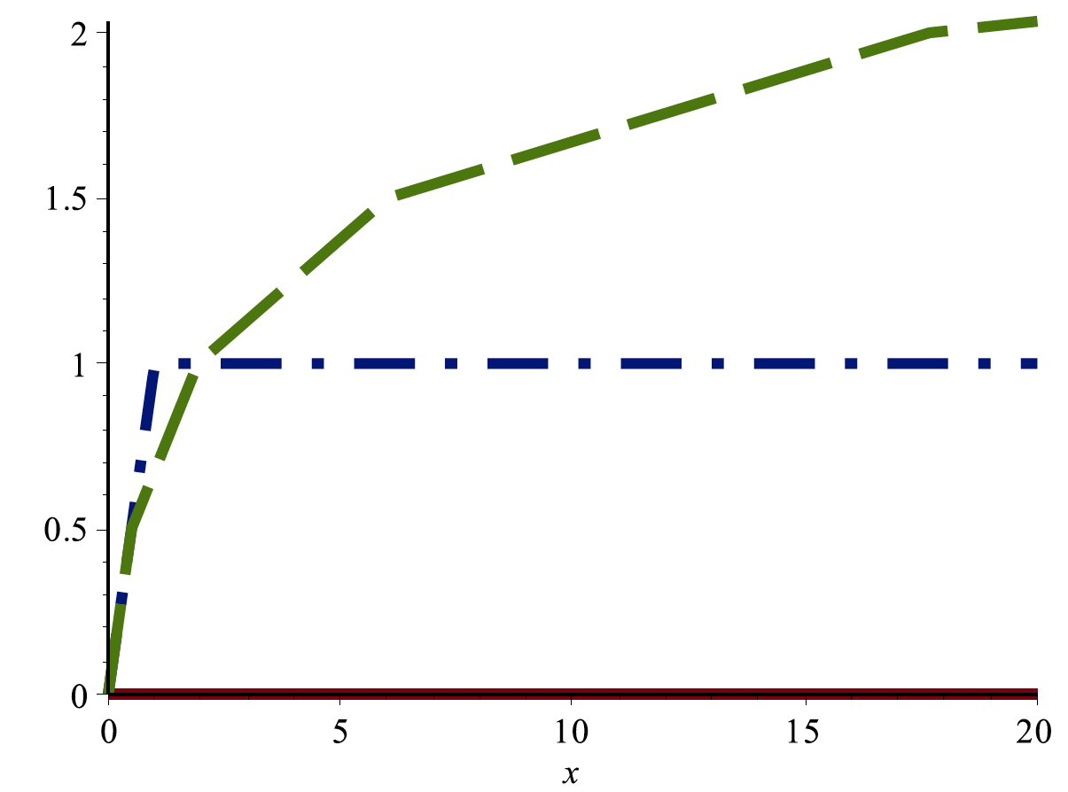
Figure 1: The solid curve represents $\lim_{n\to\infty}(T_{-\operatorname{v}})^{n}x$, the dashed dotted curve represents $\lim_{n\to\infty}(\operatorname{v}+T)^{n}x$, and the dashed curve represents $\lim_{n\to\infty}T^{n}x+n\operatorname{v}$, when $\alpha=0.5$ and $\beta=1$.

Figure 1 provides a plot of the functions defined by 22, 23 and 24 that illustrates that they are pairwise distinct.

4 The Douglas–Rachford operator for two affine subspaces

Unless otherwise stated we assume from now on that

$$A\text{~{}~{}and~{}~{}}B\text{~{}~{}are maximally monotone operators on~{}~{}}X.$$

The Attouch–Théra dual pair of $(A,B)$ (see [1]) is the pair $(A,B)^{*}:=(A^{-1},B^{-\ovee})$, where

(25) $$A^{\ovee}:=(-\operatorname{Id})\circ A\circ(-\operatorname{Id})\quad{\text{and}}\quad A^{-\ovee}:=(A^{-1})^{\ovee}=(A^{\ovee})^{-1}.$$

We shall use

(26) $$Z:=Z_{(A,B)}=(A+B)^{-1}(0)\qquad\text{and }\qquad K:=K_{(A,B)}=(A^{-1}+B^{-\ovee})^{-1}(0),$$

to denote the primal and dual solutions respectively (see e.g. [4]).

The normal problem associated with the ordered pair $(A,B)$ (see [8]) is to find $x\in X$ such that

(27) $$0\in{{}_{\operatorname{v}}A}x+B_{\operatorname{v}}x=Ax-\operatorname{v}+B(x-\operatorname{v}),$$

where

(28) $$\operatorname{v}=P_{\overline{\operatorname{ran}}(\operatorname{Id}-T)},$$

and $T=T_{(A,B)}$ is defined by 1. We recall (see [13, Lemma 2.6(iii)] and [4, Corollary 4.9]) that

(29) $$Z=J_{A}(\operatorname{Fix}T)\quad\text{and}\quad K=(\operatorname{Id}-J_{A})(\operatorname{Fix}T),$$

and that $T$ is self-dual (see [16, Lemma 3.6 on page 133] and [4, Corollary 4.3]), i.e.,

(30) $$T_{(A,B)}=T_{(A,B)^{*}}=T_{(A^{-1},B^{-\ovee})}.$$

The normal pair associated with the ordered pair $(A,B)$ is the pair $(_{\operatorname{v}}A,B_{\operatorname{v}})$ and the normal Douglas-Rachford operator is $T_{\left({}_{\operatorname{v}}A,B_{\operatorname{v}}\right)}$. Using [8, Proposition 2.24] we have

(31) $$T_{(_{\operatorname{v}}A,B_{\operatorname{v}})}=T_{-\operatorname{v}}.$$

The set of normal solutions is $Z_{\operatorname{v}}:=Z_{\left({}_{\operatorname{v}}A,B_{\operatorname{v}}\right)}$ and the set of dual normal solutions is $K_{\operatorname{v}}:=K_{\left({}_{\operatorname{v}}A,B_{\operatorname{v}}\right)}$.

Lemma 4.1.

The following hold:

1. $Z_{\operatorname{v}}=J_{{}_{\operatorname{v}}A}(\operatorname{Fix}(T_{-\operatorname{v}}))=J_{(-\operatorname{v}+A)}(\operatorname{Fix}(T_{-\operatorname{v}}))=J_{A}(\operatorname{Fix}(T_{-\operatorname{v}})+\operatorname{v})=J_{A}(\operatorname{Fix}(\operatorname{v}+T))$.

2. $K_{\operatorname{v}}=(\operatorname{Id}-J_{{}_{\operatorname{v}}A})(\operatorname{Fix}(T_{-\operatorname{v}}))=(\operatorname{Id}-J_{(-\operatorname{v}+A)})(\operatorname{Fix}(T_{-\operatorname{v}}))$.

3. $K_{\operatorname{v}}\neq\varnothing\iff Z_{\operatorname{v}}\neq\varnothing\iff\operatorname{v}\in\operatorname{ran}(\operatorname{Id}-T)$.

Proof. (i): Apply 29 to the normal pair $(_{\operatorname{v}}A,B_{\operatorname{v}})$ and use 31 and 3. Now apply [5, Proposition 23.15(ii)]. The last equality follows from Lemma 2.1(i). (ii): Apply 29 to the normal pair $(_{\operatorname{v}}A,B_{\operatorname{v}})$ then use 31 and [5, Proposition 23.15(iii)]. (iii): The first equivalence follows from applying [4, Proposition 2.4(v)] to the normal pair $(_{\operatorname{v}}A,B_{\operatorname{v}})$. Now combine Lemma 2.1(ii) and (i). $\hfill\quad\blacksquare$

In the following we assume that

(32) $$\operatorname{v}=P_{\overline{\operatorname{ran}}{(\operatorname{Id}-T)}}0\in{{\operatorname{ran}}\left(\operatorname{Id}-T\right)},$$

that

(33) $$U\text{~{}~{}and~{}~{}}V\text{~{}~{}are nonempty closed convex subsets of~{}~{}}X$$

and that

(34) $$A=N_{U}\text{~{}~{}and~{}~{}}B=N_{V}.$$

Using [5, Example 23.4], 1 becomes

(35) $$T_{{U},{V}}:=T_{(N_{U},N_{V})}=\operatorname{Id}-P_{U}+P_{V}R_{U},$$

where $R_{U}=2P_{U}-\operatorname{Id}$. In this case (see [8, Proposition 3.16])

(36) $$\operatorname{v}=P_{\overline{U-V}}0,$$

or equivalently

(37) $$-\operatorname{v}\in N_{\overline{U-V}}(\operatorname{v}).$$

The normal problem now is to find $x\in X$ such that

(38) $$0\in N_{U}x-\operatorname{v}+N_{V}(x-\operatorname{v}).$$

Lemma 4.2.

Let $w\in X$. Then the following hold:

1. $J_{-w+N_{U}}=J_{N_{U}}(\cdot+w)=P_{U}(\cdot+w)$.

2. $J_{N_{U}(\cdot-w)}=w+J_{N_{U}}(\cdot-w)=w+P_{U}(\cdot-w)$.

3. $N_{V}(\cdot-w)=N_{w+V}$.

4. Suppose that $U$ is an affine subspace and and that $w\in(\operatorname{par}U)^{\perp}$. Then $(\forall\alpha\in\mathbb{R})$$(\forall x\in X)$ $P_{U}(x+\alpha w)=P_{U}x$.

Proof. (i) and(ii): See [5, Proposition 23.15(ii) and (iii) and Example 23.4]. (iii): One can easily verify that $(\forall w\in X)$ we have $\iota_{V}(\cdot-w)=\iota_{w+V}$. Therefore $N_{V}(\cdot-w)={\partial}\iota_{V}(\cdot-w)={\partial}\iota_{w+V}=N_{w+V}$. (iv): Let $a\in U$. Then $U=a+\operatorname{par}U$. Using 3.1, we have $(\forall\alpha\in\mathbb{R})$$(\forall x\in X)$ $P_{U}(x+\alpha w)=P_{a+\operatorname{par}U}(x+\alpha w)=a+P_{\operatorname{par}U}(x+\alpha w-a)=a+P_{\operatorname{par}U}(x-a)+\alpha P_{\operatorname{par}U}w=a+P_{\operatorname{par}U}(x-a)=P_{a+\operatorname{par}U}x=P_{U}x$. $\hfill\quad\blacksquare$

Proposition 4.3.

Suppose that $U$ and $V$ are closed affine subspaces of $X$ and that $T=T_{{U},{V}}$. Then the following hold:

1. T is affine and $T=\operatorname{Id}-P_{U}-P_{V}+2P_{V}P_{U}$.

2. $\operatorname{v}\in(\operatorname{par}U)^{\perp}\cap(\operatorname{par}V)^{\perp}.$

3. $(\forall x\in X)$ $(\forall\alpha\in\mathbb{R})$ $P_{U}x=P_{U}(x+\alpha\operatorname{v})$.

4. $(\forall x\in X)$ $(\forall\alpha\in\mathbb{R})$ $P_{V}x=P_{V}(x+\alpha\operatorname{v})$.

5. $T_{-\operatorname{v}}=\operatorname{v}+T=T_{N_{U},N_{V}(\cdot-\operatorname{v})}=T_{{U},{\operatorname{v}+V}}$.

6. $Z_{\operatorname{v}}=U\cap(\operatorname{v}+V)$.

7. $K_{\operatorname{v}}=(\operatorname{par}U)^{\perp}\cap(\operatorname{par}V)^{\perp}$.

8. $\operatorname{Fix}(T_{-\operatorname{v}})=\operatorname{Fix}(\operatorname{v}+T)=Z_{\operatorname{v}}+K_{\operatorname{v}}=(U\cap(\operatorname{v}+V))+((\operatorname{par}U)^{\perp}\cap(\operatorname{par}V)^{\perp})$.

Proof. (i): Note that $J_{A}=P_{U}$ and $J_{B}=P_{V}$ are affine (see e.g. [5, Corollary 3.20(i)]). Using 35 we have $T=\operatorname{Id}-P_{U}+P_{V}(2P_{U}-\operatorname{Id})=\operatorname{Id}-P_{U}+2P_{V}P_{U}-P_{V}$. Since the class of affine operators is closed under addition, subtraction and composition we deduce that $T$ is affine.

(ii): It follows from [6, Proposition 2.7 & Remark 2.8(ii)] that $\operatorname{v}\in(\operatorname{rec}U)^{\oplus}\cap(\operatorname{rec}V)^{\ominus}=(\operatorname{par}U)^{\perp}\cap(\operatorname{par}V)^{\perp},$ where the last equality follows from [5, Proposition 6.22 and Proposition 6.23(v)].

(iii) and (iv): Combine (ii) with 4.2(iv).

(v) It follows from (iv) with $\alpha$ replaced by $-1$, and 4.2(ii) that $J_{N_{V}(\cdot-\operatorname{v})}=\operatorname{v}+P_{V}(\cdot-\operatorname{v})=\operatorname{v}+P_{V}$. Consequently, using 3.2(v) and 1 we have $T_{-\operatorname{v}}=\operatorname{v}+T=\operatorname{Id}-P_{U}+\operatorname{v}+P_{V}R_{U}=T_{N_{U},N_{V}(\cdot-\operatorname{v})}$. Finally, 4.2(iii) implies that $T_{N_{U},N_{V}(\cdot-\operatorname{v})}=T_{N_{U},N_{\operatorname{v}+V}}=T_{U,\operatorname{v}+V}$.

(vi): See [8, Proposition 3.16].

(vii): Let $z\in U\cap(\operatorname{v}+V)=Z_{\operatorname{v}}$ and note that, as subdifferential operators, $N_{U}$ and $N_{V}$ are paramonotone (see, e.g., [20]) and so are the translated operators $-\operatorname{v}+N_{U}$ and $N_{V}(\cdot-\operatorname{v})$. Therefore, in view of [4, Remark 5.4] and (ii) we have

$$K_{\operatorname{v}} =(-\operatorname{v}+N_{U}z)\cap(-N_{V}(z-\operatorname{v}))=(-\operatorname{v}+(\operatorname{par}U)^{\perp})\cap(\operatorname{par}V)^{\perp}$$

(39) $$=(\operatorname{par}U)^{\perp}\cap(\operatorname{par}V)^{\perp}.$$

(viii): Since $-\operatorname{v}+N_{U}$ and $N_{V}(\cdot-\operatorname{v})$ are paramonotone, it follows from (v), (vii) and [4, Corollary 5.5] applied to the normal pair $(_{\operatorname{v}}A,B_{\operatorname{v}})$ that $\operatorname{Fix}(T_{-\operatorname{v}})=\operatorname{Fix}(\operatorname{v}+T)=Z_{\operatorname{v}}+K_{\operatorname{v}}$. Now combine with (vi) and (vii). $\hfill\quad\blacksquare$

We are now ready for our main result. It illustrates that, even in the inconsistent case, the “shadow sequence” $(P_{U}T^{n}x)_{n\in\mathbb{N}}$ behaves extremely well because it converges to a normal solution without prior knowledge of the infimal displacement vector. The proof of 4.4 relies on the work leading up to this point as well as the convergence analysis of the consistent case in [3].

Theorem 4.4 (Douglas-Rachford algorithm for two affine subspaces).

Let $x\in X$. Then $(\forall n\in\mathbb{N})$ we have

(40) $$P_{U}T^{n}x=P_{U}(T^{n}x+n\operatorname{v})=P_{U}((T_{-\operatorname{v}})^{n}x)=P_{U}T^{n}_{U,\operatorname{v}+V}=J_{-\operatorname{v}+N_{U}}((T_{-\operatorname{v}})^{n}x),$$

and

(41) $$P_{U}T^{n}x\to P_{Z_{\operatorname{v}}}x=P_{U\cap(\operatorname{v}+V)}x.$$

Moreover, if $\operatorname{par}U+\operatorname{par}V$ is closed (as is always the case when $X$ is finite-dimensional) then the convergence is linear with rate being the cosine of the Friedrichs angle

(42) $$c_{F}(\operatorname{par}U,\operatorname{par}V):=\sup_{\small\begin{subarray}{c}u\in\operatorname{par}U\cap W^{\perp}\cap{\operatorname{ball}(0;1)}\\ v\in\operatorname{par}V\cap W^{\perp}\cap{\operatorname{ball}(0;1)}\end{subarray}}{\lvert\langle u,v\rangle\rvert}<1,$$

where $W=\operatorname{par}U\cap\operatorname{par}V$ and $\operatorname{ball}(0;1)$ is the closed unit ball.

Proof. Let $n\in\mathbb{N}$. Using 4.3(iii) with $(x,\alpha)$ replaced by $(T^{n}x,n)$ we learn that $P_{U}T^{n}x=P_{U}(T^{n}x+n\operatorname{v})$. Now combine with 3.2(iv) to get the second identity. The third identity follows from applying 4.3(v). Finally note that using the first identity, 4.3(iii) with $(x,\alpha)$ replaced by $((T_{-\operatorname{v}})^{n}x,1)$ and 4.2(i) we learn that $P_{U}T^{n}x=P_{U}((T_{-\operatorname{v}})^{n}x+\operatorname{v})=J_{-\operatorname{v}+N_{U}}((T_{-\operatorname{v}})^{n}x)$. Now we prove 41. It follows from 32, 4.1(iii) and 4.3(vi) that $Z_{\operatorname{v}}=U\cap(\operatorname{v}+V)\neq\varnothing$. Now apply [3, Corollary 4.5]. $\hfill\quad\blacksquare$

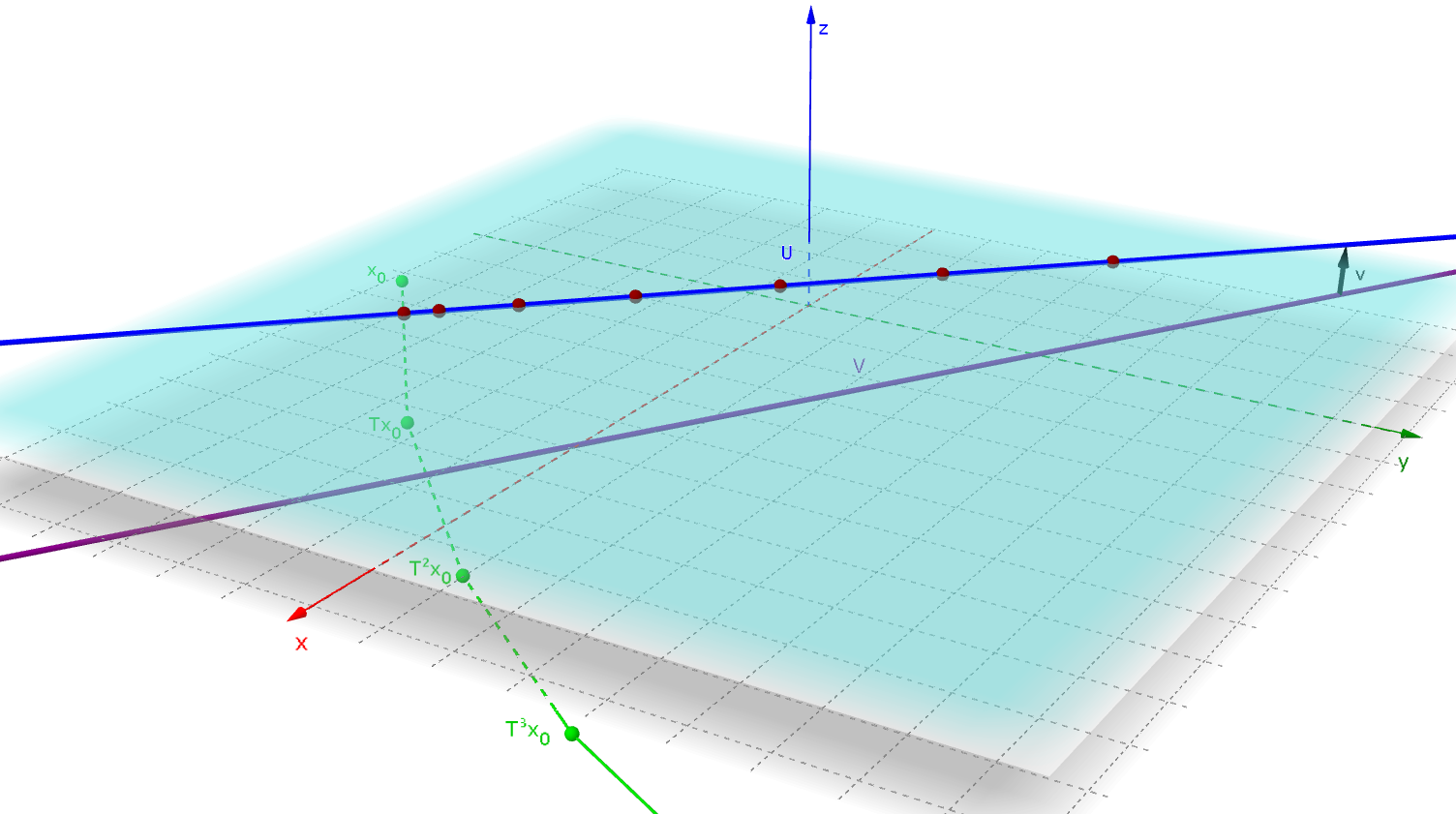
Figure 2: Two nonintersecting affine subspaces $U$ (blue line) and $V$ (purple line) in $\mathbb{R}^{3}$. Shown are also the first few iterates of $(T^{n}x_{0})_{n\in\mathbb{N}}$ (green points) and $(P_{U}T^{n}x_{0})_{n\in\mathbb{N}}$ (red points).

Figure 2 shows a Geogebra snapshot [15] of the Douglas–Rachford iterates and its shadows for two nonintersecting nonparallel lines $U$ and $V$ in $\mathbb{R}^{3}$.

The following result is known (see e.g., [11, Corollary 1.5] and [2, Corollary 2.3]). We include a simple proof for completeness in Appendix D.

Proposition 4.5.

Suppose that $T:X\to X$ be firmly nonexpansive, and that $\operatorname{v}=P_{\overline{\operatorname{ran}}(\operatorname{Id}-T)}0\in{\operatorname{ran}}(\operatorname{Id}-T)$. Then

(43) $$(\forall x\in X)\quad T^{n}x-T^{n+1}x\to\operatorname{v}.$$

Proposition 4.6 (When only one set is an affine subspace).

Suppose that $U$ is an affine subspace of $X$, and that $T=T_{{U},{V}}$. Then for every $x\in X$ the sequence $(P_{U}T^{n}x)_{n\in\mathbb{N}}$ is asymptotically regular, i.e., $P_{U}T^{n}x-P_{U}T^{n+1}x\to 0$.

Proof. Using [6, Remark 2.8(ii)] we have $\operatorname{v}\in(\operatorname{par}U)^{\perp}$. It follows from 4.2(iv) applied with $(x,\alpha)$ replaced by $(T^{n+1}x,1)$ and 4.5 that

(44) $$\lVert P_{U}T^{n}x-P_{U}T^{n+1}x\rVert=\lVert P_{U}T^{n}x-P_{U}(T^{n+1}x+\operatorname{v})\rVert\leq\lVert T^{n}x-T^{n+1}x-\operatorname{v}\rVert\to 0,$$

as claimed. $\hfill\quad\blacksquare$

Example 4.7.

(The dual shadows) Consider the case when $U$ and $V$ are affine subspaces of $X$ such that $U\cap V=\varnothing$. Set $\widetilde{A}:=N_{U}^{-1}$ and $\widetilde{B}:=N_{V}^{-\ovee}$. Then $\widetilde{A}^{-1}=N_{U}$, $\widetilde{B}^{-\ovee}=N_{V}$, and using 30 we have $T_{(\widetilde{A},\widetilde{B})}=T_{(\widetilde{A}^{-1},\widetilde{B}^{-\ovee})}=T_{{U},{V}}$. Moreover the inverse resolvent identity (see, e.g., [24, Lemma 12.14]) implies that $(\forall x\in X)$ $J_{\widetilde{A}}T^{n}x=(\operatorname{Id}-P_{U})T^{n}x=T^{n}x-P_{U}T^{n}x$. Note that $K=U\cap V=\varnothing$, hence by 29 and 30 $\operatorname{Fix}T_{(\widetilde{A},\widetilde{B})}=\varnothing$. Using [22, Corollary 6(a)] we learn that for every $x\in X$ we have $\lVert T^{n}x\rVert\to\infty$. Moreover, in view of 32, using [6, Theorem 3.13(iii)] we know that for every $x\in X$ we have $(P_{U}T^{n}x)_{n\in\mathbb{N}}$ is a bounded sequence. Therefore, $\lVert J_{\widetilde{A}}T^{n}x\rVert=\lVert T^{n}x-P_{U}T^{n}x\rVert\geq\lVert T^{n}x\rVert-\lVert P_{U}T^{n}x\rVert\to\infty$.

We conclude with the following example which shows that for two affine (but not normal cone) operators the shadows need not converge.

Example 4.8.

Suppose that $X=\mathbb{R}^{2}$ and let $S:\mathbb{R}^{2}\to\mathbb{R}^{2}:(x_{1},x_{2})\mapsto(-x_{2},x_{1})$, be the counter-clockwise rotator by $\pi/2$. Let $b\in\mathbb{R}^{2}\smallsetminus\left\{(0,0)\right\}$. Suppose that $A:=S$ and set $B:=-S+b$. Then $\operatorname{zer}A\neq\varnothing$, $\operatorname{zer}B\neq\varnothing$ yet $\operatorname{zer}(A+B)=\varnothing$. Moreover, $\operatorname{v}=(\operatorname{Id}+S)(b)$, the set of normal solutions $Z_{\operatorname{v}}=\mathbb{R}^{2}$ and for every $x\in\mathbb{R}^{2}$ we have $\lVert J_{A}T^{n}x\rVert\to\infty$.

Proof. Let $x\in\mathbb{R}^{2}$ and note that $S$ and $-S$ are both linear, continuous, single-valued, monotone and $S^{2}=(-S)^{2}=-\operatorname{Id}$. It follows from [8, Proposition 2.10] that $J_{A}x=J_{S}x=\tfrac{1}{2}(\operatorname{Id}-S)x=\tfrac{1}{2}(x-Sx)$. Similarly using [5, Proposition 23.15(ii)] we can see that $J_{B}x=\tfrac{1}{2}(x-b+Sx-Sb)$. Therefore we have $R_{A}x=-Sx$ and $R_{B}x=-b+Sx-Sb$. Hence $R_{B}R_{A}x=S(-Sx)-Sb-b=-S^{2}x-Sb-b=x-Sb-b=x-(\operatorname{Id}+S)b$. Consequently we have

(45) $$(\forall x\in\mathbb{R}^{2})\quad Tx=\tfrac{1}{2}(\operatorname{Id}+R_{B}R_{A})x=x-\tfrac{1}{2}(\operatorname{Id}+S)b.$$

It follows from 45 that $\operatorname{ran}(\operatorname{Id}-T)=\{\tfrac{1}{2}(\operatorname{Id}+S)b\}$, hence $\operatorname{v}=\tfrac{1}{2}(\operatorname{Id}+S)b$ and $Tx=x-\operatorname{v}$. Therefore, using 3.2(v) $\operatorname{Fix}(\operatorname{v}+T)=\operatorname{Fix}(T_{-\operatorname{v}})=\mathbb{R}^{2}$. Moreover, using 29 and 31 applied to the normal pair $\left({}_{\operatorname{v}}A,B_{\operatorname{v}}\right)$ we learn that $Z_{\operatorname{v}}=J_{{}_{\operatorname{v}}A}(\operatorname{Fix}(T_{-\operatorname{v}}))=\mathbb{R}^{2}$. In view of 2.4(i) we have $T^{n}x=x-n\operatorname{v}$. Hence, using that $J_{A}$ is linear, we get $J_{A}T^{n}x=J_{A}(x-n\operatorname{v})=J_{A}x-nJ_{A}\operatorname{v}$. Now $J_{A}\operatorname{v}=\frac{1}{2}(\operatorname{Id}-S)(\frac{1}{2}(\operatorname{Id}+S)b)=\frac{1}{2}b\neq(0,0)$, which completes the proof. $\hfill\quad\blacksquare$

Appendix A

Proof of 2.3. Using that $P_{C}$ is firmly nonexpansive we have $\lVert c-P_{C}0\rVert^{2}=\lVert P_{C}c-P_{C}0\rVert^{2}\leq\lVert c-0\rVert^{2}-\lVert(\operatorname{Id}-P_{C})c-(\operatorname{Id}-P_{C})0\rVert^{2}=\lVert c\rVert^{2}-\lVert c-P_{C}c+P_{C}0\rVert^{2}=\lVert c\rVert^{2}-\lVert P_{C}0\rVert^{2}=0$. $\hfill\quad\blacksquare$

Appendix B

Proof of 2.7. Clearly

(46) $$\operatorname{Id}-T=P_{\left[\alpha,\beta\right]}:\mathbb{R}\to\mathbb{R}:x\mapsto\begin{cases}\alpha,&\text{~{}\rm if~{}}x\leq\alpha;\\ x,&\text{~{}\rm if~{}}\alpha<x\leq\beta;\\ \beta,&\text{~{}\rm if~{}}x>\beta.\end{cases}$$

Therefore, $\operatorname{ran}(\operatorname{Id}-T)=[\alpha,\beta]$, and consequently $\operatorname{v}=\alpha$. Moreover

(47) $$(\forall x\in\mathbb{R})\quad x\geq Tx+\alpha\geq T^{2}x+2\alpha\geq\cdots\geq T^{n}x+n\alpha\geq\cdots.$$

It is clear from Example 2.5 that

(48) $$\operatorname{Fix}(\operatorname{v}+T)=\left]-\infty,\alpha\right].$$

The statement for $\operatorname{Fix}T_{-\operatorname{v}}$ then follows from combining 48 and Lemma 2.1(i). The convergence of the sequence follows from Example 2.5 or 2.6(i). Now we prove 13. We claim that

(49) $$T^{n}:\mathbb{R}\to\mathbb{R}:x\mapsto\begin{cases}x-n\alpha,&\text{~{}\rm if~{}}x\leq\alpha;\\ (1-n)\alpha,&\text{~{}\rm if~{}}\alpha<x\leq\beta;\\ x-n\beta,&\text{~{}\rm if~{}}x>\beta\text{~{}\rm and~{}}n\leq\lfloor{x}/{\beta}\rfloor;\\ \min\left\{\alpha,x-\Big{\lfloor}\tfrac{x}{\beta}\Big{\rfloor}\beta\right\}+\left(\Big{\lfloor}\tfrac{x}{\beta}\Big{\rfloor}-n\right)\alpha,&\text{~{}\rm if~{}}x>\beta\text{~{}\rm and~{}}n>\lfloor{x}/{\beta}\rfloor.\end{cases}$$

Using induction it is easy to verify the cases when $x\leq\alpha$ and when $\alpha<x\leq\beta$. Now we focus on the case when $x>\beta$. Set

(50) $$K:=\lfloor x/\beta\rfloor\text{~{}~{}and~{}~{}}r:=x-K\beta,$$

and note that $x=K\beta+r$, $K\in\{1,2,3,\ldots\}$ and $0\leq r<\beta$. In view of 47, if $n\in\{0,1,2,3,\ldots,K\}$ we get $T^{n}x=x-n\beta=(K-n)\beta+r$. In particular,

(51) $$T^{K}x=x-\lfloor x/\beta\rfloor\beta=r.$$

If $n>K$ we examine two cases. Case 1: $0\leq r\leq\alpha$. It follows from 51 and 12 that $(\forall n\geq K)$ $T^{n}x=r+(K-n)\alpha$. Case 2: $\alpha<r<\beta$. Note that $T^{K+1}x=0$, therefore using 51 and 12 we have $(\forall n>K)$ $T^{n}x=(K+1-n)\alpha=\alpha+(K-n)\alpha$, which proves 49. Now 13 follows from 49 because $\operatorname{v}=\alpha$. Letting $n\to\infty$ in 13 yields 14. Note that $\min\{\alpha,x-\lfloor\tfrac{x}{\beta}\rfloor\beta\}\geq 0$ and $\lfloor\tfrac{x}{\beta}\rfloor\geq 1$. By considering cases $(K=1$ and $K\geq 1)$, 14 implies that $\lim_{n\to\infty}(T^{n}x_{0}+n\operatorname{v})=\min\{\alpha,x-\lfloor\tfrac{x}{\beta}\rfloor\beta\}+\lfloor\tfrac{x}{\beta}\rfloor\alpha>\alpha\not\in\left]-\infty,\alpha\right]=\operatorname{Fix}(\operatorname{v}+T)$.

$\hfill\quad\blacksquare$

Appendix C

Proof of 3.3. Considering cases, we easily check that

(52) $$\operatorname{Id}-T\colon\mathbb{R}\to\mathbb{R}:x\mapsto\left(1-\alpha\right)\max\left\{x,\beta\right\}+\alpha\beta\geq\beta>0.$$

Hence $\operatorname{Fix}T=\varnothing$ and $\operatorname{v}=\beta$ as claimed. Moreover, using 52 one can verify that

(53) $$(\forall x\in X)\quad x\geq Tx+\beta>\cdots\geq T^{n}x+n\beta\geq T^{n+1}x+(n+1)\beta\geq\cdots.$$

We also verify that

(54) $$(\forall x\in\mathbb{R})\quad T_{-\operatorname{v}}:\mathbb{R}\to\mathbb{R}:x\mapsto\max\left\{x,0\right\}\alpha+\min\left\{x,0\right\}.$$

We now prove 19 by induction. Let $x\in\mathbb{R}$.

Clearly when $n=0$ the base case holds true. Now suppose that for some $n\in\mathbb{N}$ 19 holds. If $x\leq 0$ then $\left(T_{-\operatorname{v}}\right)^{n}x=x\leq 0$, and therefore, 54 implies that $\left(T_{-\operatorname{v}}\right)^{n+1}x=T_{-\operatorname{v}}(\left(T_{-\operatorname{v}}\right)^{n}x)=T_{-\operatorname{v}}x=x$. Similarly we have $x>0\Rightarrow\alpha^{n}x=\left(T_{-\operatorname{v}}\right)^{n}x>0$, and consequently 54 implies that $\left(T_{-\operatorname{v}}\right)^{n+1}x=T_{-\operatorname{v}}(\left(T_{-\operatorname{v}}\right)^{n}x)=T_{-\operatorname{v}}(\alpha^{n}x)=\alpha^{n+1}x$. The proof of 20 follows from combining 19 and Lemma 2.1(iii). Now we turn to 21. We consider two cases.
Case 1: $x\leq\beta$. It is obvious using the definition of ${T}$ that $(\forall n\in\mathbb{N})$ ${T}^{n}x=x-n\beta$.
Case 2: $x>\beta$. Let $n\in\mathbb{N}$ be such that $T^{n}x>\beta$. By 53 and 18 we have

$$T^{n+1}x =\alpha^{n+1}x-(\alpha^{n+1}+\alpha^{n}+\cdots+\alpha)\beta=\alpha^{n+1}x-\frac{\alpha(1-\alpha^{n+1})}{1-\alpha}\beta$$

(55) $$=\alpha^{n+1}\left(\frac{(1-\alpha)x+\alpha\beta}{1-\alpha}\right)-\frac{\alpha}{1-\alpha}\beta.$$

In view of 53 there exists a unique integer, say, $q(x)\in\{1,2,\ldots\}$ that satisfies ${T}^{q(x)-1}x>\beta$ and ${T}^{q(x)}x\leq\beta$. Since $0<\alpha<1$, using Appendix C we have

$$T^{q(x)}x\leq\beta \iff\alpha^{q(x)}\left(\frac{(1-\alpha)x+\alpha\beta}{1-\alpha}\right)-\frac{\alpha}{1-\alpha}\beta\leq\beta$$

$$\iff\alpha^{q(x)}\left(\frac{(1-\alpha)x+\alpha\beta}{1-\alpha}\right)\leq\frac{\beta}{1-\alpha}\iff\alpha^{q(x)}\left((1-\alpha)x+\alpha\beta\right)\leq\beta$$

$$\iff\alpha^{q(x)}\leq\frac{\beta}{(1-\alpha)x+\alpha\beta}\iff{q(x)\geq{\log_{\alpha}\frac{\beta}{\alpha\beta+(1-\alpha)x}}}.$$

Consequently, $q(x)=\left\lceil{\log_{\alpha}\frac{\beta}{\alpha\beta+(1-\alpha)x}}\right\rceil$. At this point, since ${T}^{q(x)}x\leq\beta$, we must have $(\forall n\geq q(x))$ ${T}^{n}x={T}^{q(x)}x-(n-q(x))\beta$, which proves 21. The formulae 22, 23 and 24 are direct consequences of 19, 20 and 21, respectively. To prove the last claim note that if $S:\mathbb{R}\to\mathbb{R}$ is such that for every $n\in\mathbb{N}$ we have $S^{n}=T^{n}+n\operatorname{v}$, then setting $n=1$ must yield

(56) $$S=\operatorname{v}+T\colon\mathbb{R}\to\mathbb{R}:x\mapsto\begin{cases}x,&x\leq\beta;\\ \alpha\left(x-\beta\right)+\beta,&x>\beta.\end{cases}$$

Now compare 20 and 21. $\hfill\quad\blacksquare$

Appendix D

Proof of 4.5. Let $y_{0}\in\operatorname{Fix}(\operatorname{v}+T)$ and note that 2.4(iv) implies that $(\forall n\in\mathbb{N})~{}(\operatorname{Id}-T)T^{n}y_{0}=\operatorname{v}$. Since $T$ is firmly nonexpansive, it follows from 2.4(vi) and [5, Proposition 5.4(ii)] that

$$\lVert T^{n}x-T^{n+1}x-\operatorname{v}\rVert^{2} =\lVert(\operatorname{Id}-T)T^{n}x-(\operatorname{Id}-T)T^{n}y_{0}\rVert^{2}$$

$$\leq\lVert T^{n}x-T^{n}y_{0}\rVert^{2}-\lVert T^{n+1}x-T^{n+1}y_{0}\rVert^{2}$$

$$=\lVert T^{n}x+n\operatorname{v}-y_{0}\rVert^{2}-\lVert T^{n+1}x+(n+1)\operatorname{v}-y_{0}\rVert^{2}\to 0.$$

$\hfill\quad\blacksquare$

References

[1]
H. Attouch and M. Théra,
A general duality principle for the sum of two operators,
Journal of Convex Analysis 3 (1996), 1–24.
[2]
J.B. Baillon, R.E. Bruck and S. Reich,
On the asymptotic behavior of nonexpansive
mappings and semigroups in Banach spaces.
Houston Journal of Mathematics 4 (1978), 1–9.
[3]
H.H. Bauschke, J.Y. Bello Cruz, T.T.A. Nghia, H.M. Phan and X. Wang:
The rate of linear convergence of the Douglas-Rachford algorithm
for subspaces is the cosine of the Friedrichs angle,
Journal of Approximation Theory 185 (2014), 63–79.
[4] H.H. Bauschke, R.I. Boţ,
W.L. Hare and W.M. Moursi,
Attouch–Théra
duality revisited: paramonotonicity and operator splitting,
Journal of Approximation Theory 164 (2012), 1065–1084.
[5]
H.H. Bauschke and P.L. Combettes,
Convex Analysis and Monotone
Operator Theory in Hilbert Spaces,
Springer, 2011.
[6]
H.H. Bauschke, P.L. Combettes
and D.R. Luke,
Finding best approximation pairs relative to two
closed convex sets in Hilbert spaces,
Journal of Approximation Theory
127 (2004), 178–192.
[7]
H.H. Bauschke, F. Deutsch, H. Hundal
and S.-H. Park: Accelerating the convergence of
the method of alternating projections,
Transactions of the American Mathematical Society
355 (2003), 3433–3461.
[8]
H.H. Bauschke, W.L. Hare and W.M. Moursi, Generalized solutions
for the sum of two maximally monotone operators,
SIAM Journal on Control and Optimization 52 (2014),
1034–1047.
[9]
J.M. Borwein and J.D. Vanderwerff,
Convex Functions,
Cambridge University Press, 2010.
[10]
H. Brezis,
Operateurs Maximaux Monotones et
Semi-Groupes de Contractions dans les Espaces de Hilbert,
North-Holland/Elsevier, 1973.
[11]
R.E. Bruck and S. Reich,
Nonexpansive projections and resolvents of accretive operators in
Banach spaces, Houston Journal of Mathematics
3 (1977), 459–470.
[12]
R.S. Burachik and A.N. Iusem,
Set-Valued Mappings and Enlargements
of Monotone Operators,
Springer-Verlag, 2008.
[13]
P.L. Combettes,
Solving monotone inclusions via compositions of nonexpansive averaged
operators,
Optimization 53 (2004), 475–504.
[14]
L. Demanet and X. Zhang,
Eventual linear convergence of the Douglas–Rachford iteration
for basis pursuit, to appear in Mathematics of Compution, AMS.
[16]
J. Eckstein,
Splitting Methods for Monotone Operators with
Applications to Parallel Optimization,
Ph.D. thesis, MIT, 1989.
[17]
J. Eckstein and D.P. Bertsekas,
On the Douglas–Rachford splitting method
and the proximal point algorithm for maximal monotone
operators,
Mathematical Programming (Series A) 55 (1992), 293–318.
[18]
R. Hesse and D.R. Luke,
Nonconvex notions of regularity and
convergence of fundamental
algorithms for feasibility problems,
SIAM Journal on Optimization 23 (2013), 2397–2419.
[19]
R. Hesse, D.R. Luke, and P. Neumann,
Alternating projections and Douglas-Rachford for
sparse affine feasibility,
IEEE Transactions on Signal Processing, vol. 62 (2014),
No. 18.
[20]
A.N. Iusem,
On some properties of paramonotone operators,
Journal of Convex Analysis 5 (1998), 269–278.
[21]
P.L. Lions and B. Mercier, Splitting algorithms for the sum of two
nonlinear operators.
SIAM Journal on Numerical Analysis 16(6) (1979), 964–979.
[22] A. Pazy, Asymptotic behavior of contractions in
Hilbert space, Israel Journal of Mathematics 9 (1971), 235–240.
[23]
R.T. Rockafellar,
Convex Analysis,
Princeton University Press, Princeton, 1970.