Galerkin v. least-squares Petrov–Galerkin projection
in nonlinear model reduction

Abstract

Least-squares Petrov–Galerkin (LSPG) model-reduction techniques such as the Gauss–Newton with Approximated Tensors (GNAT) method have shown promise, as they have generated stable, accurate solutions for large-scale turbulent, compressible flow problems where standard Galerkin techniques have failed. However, there has been limited comparative analysis of the two approaches. This is due in part to difficulties arising from the fact that Galerkin techniques perform optimal projection associated with residual minimization at the time-continuous level, while LSPG techniques do so at the time-discrete level.

This work provides a detailed theoretical and computational comparison of the two techniques for two common classes of time integrators: linear multistep schemes and Runge–Kutta schemes. We present a number of new findings, including conditions under which the LSPG ROM has a time-continuous representation, conditions under which the two techniques are equivalent, and time-discrete error bounds for the two approaches. Perhaps most surprisingly, we demonstrate both theoretically and computationally that decreasing the time step does not necessarily decrease the error for the LSPG ROM; instead, the time step should be ‘matched’ to the spectral content of the reduced basis. In numerical experiments carried out on a turbulent compressible-flow problem with over one million unknowns, we show that increasing the time step to an intermediate value decreases both the error and the simulation time of the LSPG reduced-order model by an order of magnitude.

url]sandia.gov/ ktcarlb

1 Introduction

While modeling and simulation of parameterized systems has become an essential tool in many industries, the computational cost of executing high-fidelity simulations is infeasibly high for many time-critical applications. For example, real-time scenarios (e.g., model predictive control) require simulations to execute in seconds or minutes, while many-query scenarios (e.g., statistical inversion) can require thousands of simulations corresponding to different parameter instances of the system.

Reduced-order models (ROMs) have been developed to mitigate this computational bottleneck. First, they execute an offline stage during which computationally expensive training tasks (e.g., evaluating the high-fidelity model at several points in the parameter space) compute a representative low-dimensional ‘trial’ basis for the system state. Then, during the inexpensive online stage, these methods quickly compute approximate solutions for arbitrary points in the parameter space via projection: they compute solutions in the span of the trial basis while enforcing the high-fidelity-model residual to be orthogonal to a low-dimensional ‘test’ basis. They also introduce other approximations in the presence of general nonlinearities or non-affine parameter dependence. See Ref. [13] and references within for a survey of current methods.

By far the most popular model-reduction technique for nonlinear ordinary differential equations (ODEs) is Galerkin projection [53], wherein the test basis is set to be equal to the trial basis, which is often computed via proper orthogonal decomposition (POD) [35]. Galerkin projection can be considered continuous optimal, as the Galerkin-ROM velocity minimizes the ODE (time-continuous) residual in the $\ell^{2}$-norm. In addition, for specialized dynamical systems (e.g., Lagrangian dynamical systems), performing Galerkin projection is necessary to preserve problem structure [39, 22, 23]. However, theoretical analyses—in the form of time-continuous error bounds [45] and stability analysis [31]—as well as numerical experiments have shown that Galerkin projection can lead to significant problems when applied to general nonlinear ODEs: instability [46], inaccurate long-time responses [52, 43], and no guarantee of a priori convergence (i.e., adding basis vectors can degrade the solution) [47, Section 5]. In turbulent fluid flows, some of this poor performance can be attributed to the trial basis ‘filtering out’ small-scale modes essential for energy dissipation.

To address these shortcomings, alternative projection techniques have been developed, particularly in fluid dynamics. These include stabilizing inner products [47, 11, 38]; introducing dissipation via closure models [8, 52, 14, 57, 50] or numerical dissipation [36]; performing nonlinear Galerkin projection based on approximate inertial manifolds [41, 51, 37]; including a pressure-term representation [43, 33]; modifying the POD basis by including many modes (such that dissipative modes are captured), changing the norm [36], enabling adaptivity [14], or including basis functions that resolve a range of scales [9] or respect the attractor’s power balance [10]; and performing Petrov–Galerkin projection [28].

Alternatively, a promising new model-reduction methodology eschews Galerkin projection in favor of performing projection at the fully discrete level, i.e., after the ODE has been discretized in time [19]. This discrete-optimal method—known as least-squares Petrov–Galerkin (LSPG) projection—computes the solution that minimizes the $\ell^{2}$-norm of the (time-discrete) residual arising at each time step; this ensures that adding basis vectors yields a monotonic decrease in the least-squares objective function. When equipped with gappy POD [27] (a least-squares generalization of—and precursor to—the discrete empirical interpolation method [24]) to approximate the discrete residual as a complexity-reduction mechanism, this approach is known as the Gauss–Newton with Approximated Tensors (GNAT) method [21]. While LSPG projection does not necessarily guarantee a priori accuracy and stablility for turbulent, compressible flows, it has been computationally demonstrated to generate accurate and stable responses for such problems on which Galerkin projection yielded unstable responses [19, 20, 21].

In spite of its promise, theoretical analysis has been limited to developing consistency conditions for snapshot collection [19, 21] and discrete-time error bounds for simple time integrators [21, 3]. In particular, major outstanding questions include: (1) What are time-continuous and time-discrete representations of the Galerkin and LSPG ROMs for broad classes of time integrators? (2) Are there conditions under which the two techniques are equivalent? (3) What discrete-time error bounds are available for the two techniques for broad classes time integrators? Related to the third issue is how parameters (e.g., time step or basis dimension) for the LSPG ROM should be chosen to optimize performance. This work aims to fill this gap by performing a number of detailed theoretical and computational studies that compare Galerkin and LSPG ROMs for the two most important classes of time integrators: linear multistep methods and Runge–Kutta schemes. We summarize the most important theoretical results (which map to the three questions above) as follows:

Figure 1: Relationship between Galerkin and discrete-optimal ROMs at the time-continuous (ODE) and time-discrete (O$\Delta$E) levels. Bolded outlines imply the ROM associates with a minimum-residual solution at that time-discretization level. Dashed lines imply the relationships are valid under certain conditions (see Theorems 4.2 and 4.3).

1. Continuous and discrete representations

   • Galerkin projection and time discretization are commutative (Theorem 3.4).

   • LSPG ROMs can be derived for Runge–Kutta schemes (Section 4.1).

   • The LSPG ROM has a time-continuous (i.e., ODE) representation under certain conditions (Section 4.2, Figure 1). This ODE depends on the time step $\Delta t$.

2. Equivalence conditions

   • Galerkin and LSPG ROMs are equivalent for explicit time integrators (Corollaries 5.1 and 5.2).

   • Galerkin and LSPG ROMs are equivalent in the limit of $\Delta t\rightarrow 0$ for implicit time integrators (Theorem 5.3).

   • Galerkin ROMs are discrete optimal for symmetric-positive-definite residual Jacobians (Theorems 5.4–5.6).

3. Error analysis

   • We provide local and global a posteriori and a priori error bounds for both Galerkin and LSPG ROMs for linear multistep schemes (Section 6.1).

   • For backward differentiation formulas, we show that the LSPG ROM can yield a lower local a posteriori error bound than the Galerkin ROM (Corollary 6.4) because it solves a time-global optimization problem (over a time window) rather than a time-local optimization problem (Remark 6.9).

   • For the backward Euler time integrator, we show that an intermediate time step should yield the lowest error bound (Corollary 6.17 and Remark 6.18).

   • For the backward Euler time integrator, we show that a larger basis size leads to a smaller optimal time step for the LSPG ROM (Corollary 6.17).

   • We provide global a posteriori and a priori error bounds for both Galerkin and LSPG ROMs for Runge–Kutta schemes (Section 6.3).

Figure 1 summarizes time-continuous and time-discrete representations of the two techniques.

In addition to the above theoretical results, we present numerical results for a large-scale compressible fluid-dynamics problem with turbulence modeling characterized by over one million degrees of freedom. These results illustrate the practical significance of the above theoretical results. Critically, we show that employing an intermediate time step for the LSPG ROM can decrease both the error and the simulation time by an order of magnitude, which is a highly non-intuitive result that is of immense practical significance.

The remainder of the paper is organized as follows. Section 2 formulates the full-order model, including its representation at the time-continuous and time-discrete levels. Section 3 presents the Galerkin ROM at the continuous and discrete levels, and Section 4 does so for the LSPG ROM. In particular, we provide conditions under which the LSPG ROM has a time-continuous representation. Section 5 provides conditions under which the Galerkin and LSPG ROMs are equivalent; in particular, equivalence holds for explicit integrators (Section 5.1), in the limit of the time step going to zero for implicit integrators (Section 5.2), and for symmetric-positive-definite residual Jacobians (Section 5.3). Section 6 provides error analysis for Galerkin and LSPG ROMs for linear multistep schemes (Section 6.1), Runge–Kutta schemes (Section 6.3), and a detailed analysis in the case of backward Euler (Section 6.2). Section 7 provides detailed numerical examples that illustrate the practical importance of the analysis. Finally, Section 8 provides conclusions.

In the remainder of this paper, matrices are denoted by capitalized bold letters, vectors by lowercase bold letters, scalars by unbolded letters. The columns of a matrix $\bm{A}\in\mathbb{R}^{m\times{n}}$ are denoted by $\bm{a}_{i}\in\mathbb{R}^{m}$, $i\in\mathbb{N}({n})$ with $\mathbb{N}(a)\vcentcolon=\{1,\ldots,a\}$ such that $\bm{A}\vcentcolon=\left[\bm{a}_{1}\ \cdots\ \bm{a}_{n}\right]$. We also define $\mathbb{N}_{0}(a)\vcentcolon=\{0,\ldots,a\}$. The scalar-valued matrix elements are denoted by $a_{ij}\in\mathbb{R}$ such that $\bm{a}_{j}\vcentcolon=\left[a_{1j}\ \cdots\ a_{mj}\right]^{T}$, $j\in\mathbb{N}({n})$. A superscript denotes the value of a variable at that time instance, e.g., $\bm{{x}}^{n}$ is the value of $\bm{{x}}$ at time $n\Delta t$, where $\Delta t$ is the time step.

2 Full-order model

We begin by formulating both the time-continuous (ODE) and time-discrete (O$\Delta$E) representations of the full-order model (FOM).

2.1 Continuous representation

In this work, we consider the full-order model (FOM) to be an initial value problem characterized by a system of nonlinear ODEs

$$\frac{d\bm{{x}}}{dt} ={\bm{{f}}}(\bm{{x}},t),\qquad\bm{{x}}(0)=\bm{{x}}_{0},$$ (2.1)

where $\bm{{x}}\mathrel{\mathop{\mathchar 58\relax}}\left[0,T\right]\rightarrow\mathbb{R}^{N}$ denotes the (time-dependent) state, $\bm{{x}}_{0}\in\mathbb{R}^{N}$ denotes the initial condition, and $\bm{{f}}\mathrel{\mathop{\mathchar 58\relax}}\mathbb{R}^{N}\times\left[0,T\right]\rightarrow\mathbb{R}^{N}$ with $\left(\bm{{\xi}},\tau\right)\mapsto\bm{{f}}\left(\bm{{\xi}},\tau\right)$. This ODE can arise, for example, from applying spatial discretization (e.g., finite element, finite volume, or finite difference) to a partial differential equation with time dependence. We note that most model-reduction techniques are applied to parameterized systems wherein the velocity $\bm{{f}}$ is also parameter dependent. However, we limit our presentation to unparameterized systems for notational simplicity, as we are interested comparing Galerkin and LSPG ROMs for a given instance of the ODE.

2.2 Discrete representation

A time-discretization method is required to solve Eq. (2.1) numerically. We now characterize the full-order-model O$\Delta$E, which is the time-discrete representation of the model, for two classes of time integrators: linear multistep schemes and Runge–Kutta schemes.

2.2.1 Linear multistep schemes

A linear $k$-step method applied to numerically solve Eq. (2.1) can be expressed as

$$\sum_{j=0}^{k}\alpha_{j}\bm{{x}}^{n-j}=\Delta t\sum_{j=0}^{k}\beta_{j}\bm{{f}}\left(\bm{{x}}^{n-j},t^{n-j}\right),$$ (2.2)

where $\Delta t$ is the time step, the coefficients $\alpha_{j}$ and $\beta_{j}$ define a specific linear multistep scheme, $\alpha_{0}\neq 0$, and $\sum\limits_{j=0}^{k}\alpha_{j}=0$ is necessary for consistency. In this case, the O$\Delta$E is characterized by the following system of algebraic equations to be solved at each time instance $n\in\mathbb{N}(T/\Delta t)$:

$${\bm{{r}}}^{n}\left(\bm{{w}}^{n}\right)=0,$$ (2.3)

where $\bm{{w}}^{n}\in\mathbb{R}^{N}$ is the unknown variable and ${\bm{{r}}}^{n}\mathrel{\mathop{\mathchar 58\relax}}\mathbb{R}^{N}\rightarrow\mathbb{R}^{N}$ denotes the linear multistep residual defined as

$${\bm{{r}}}^{n}\left(\bm{{w}}\right)\vcentcolon=\alpha_{0}\bm{{w}}-\Delta t\beta_{0}\bm{{f}}(\bm{{w}},t^{n})+\sum_{j=1}^{k}\alpha_{j}\bm{{x}}^{n-j}-\Delta t\sum_{j=1}^{k}\beta_{j}\bm{{f}}\left(\bm{{x}}^{n-j},t^{n-j}\right).$$ (2.4)

Then, the state can be updated explicitly as

$$\bm{{x}}^{n}=\bm{{w}}^{n}.$$

Hence, the unknown is equal to the state. These methods are implicit if $\beta_{0}\neq 0$.

2.2.2 Runge–Kutta schemes

For an $s$-stage Runge–Kutta scheme, the O$\Delta$E is characterized by the following system of algebraic equations to be solved at each time step:

$${\bm{{r}}}^{n}_{i}\left(\bm{{w}}^{n}_{1},\ldots,\bm{{w}}^{n}_{s}\right)=0,\quad i\in\mathbb{N}(s).$$ (2.5)

Here, the Runge–Kutta residual is defined as

$${\bm{{r}}}^{n}_{i}\left(\bm{{w}}_{1},\ldots,\bm{{w}}_{s}\right)\vcentcolon=\bm{{w}}_{i}-\bm{{f}}(\bm{{x}}^{n-1}+\Delta t\sum_{j=1}^{s}a_{ij}\bm{{w}}_{j},t^{n-1}+c_{i}\Delta t),\quad i\in\mathbb{N}(s)$$ (2.6)

and the state is explicitly updated as

$$\bm{{x}}^{n}=\bm{{x}}^{n-1}+\Delta t\sum_{i=1}^{s}b_{i}\bm{{w}}^{n}_{i}.$$ (2.7)

Here, the unknowns $\bm{{w}}^{n}_{i}$ correspond to the velocity $d\bm{{x}}/dt$ at times $t^{n-1}+c_{i}\Delta t$, $i\in\mathbb{N}(s)$, and the coefficients $b_{i}$, $c_{i}$, and $a_{ij}$ define a specific Runge–Kutta scheme. These methods are explicit if $a_{ij}=0$, $\forall j\geq i$ and are diagonally implicit if $a_{ij}=0$, $\forall j>i$.

3 Galerkin ROM

This section provides the time-continuous and time-discrete representations of the Galerkin ROM, as well as key results related to optimality and commutativity of projection and time discretization.

3.1 Continuous representation

Galerkin-projection reduced-order models compute an approximate solution $\tilde{\bm{{x}}}\approx\bm{{x}}$ with $\tilde{\bm{{x}}}\in\mathbb{R}^{N}$ to Eq. (2.1) by introducing two approximations. First, they restrict the approximate solution to lie in a low-dimensional affine trial subspace $\bm{{x}}_{0}+\mathrm{Ran}\left(\bm{{\Phi}}\right)$, where $\bm{{\Phi}}\in\mathbb{R}^{N\times{p}}$ with $\bm{{\Phi}}^{T}\bm{{\Phi}}=\bm{{I}}$ denotes the given reduced basis (in matrix form) of dimension ${p}\ll N$ and $\mathrm{Ran}\left(\bm{{A}}\right)$ denotes the range of matrix $\bm{{A}}$. This basis can be computed by a variety of techniques, e.g., eigenmode analysis, POD [35], or the reduced-basis method [44, 48, 56, 42, 55]. Then, the approximate solution can be expressed as

$$\tilde{\bm{{x}}}(t)=\bm{{x}}_{0}+\bm{{\Phi}}{\hat{\bm{{x}}}}(t),$$ (3.1)

where ${\hat{\bm{{x}}}}\mathrel{\mathop{\mathchar 58\relax}}\left[0,T\right]\rightarrow\mathbb{R}^{{p}}$ denotes the (time-dependent) generalized coordinates of the approximate solution. Second, these methods substitute $\bm{{x}}\leftarrow\tilde{\bm{{x}}}$ into Eq. (2.1) and enforce the ODE residual to be orthogonal to $\mathrm{Ran}\left(\bm{{\Phi}}\right)$, which results in a low-dimensional system of nonlinear ODEs

$$\frac{d{\hat{\bm{{x}}}}}{dt} =\bm{{\Phi}}^{T}\bm{{f}}(\bm{{x}}_{0}+\bm{{\Phi}}{\hat{\bm{{x}}}},t),\qquad{\hat{\bm{{x}}}}(0)=0.$$ (3.2)

Remark 3.1

In order to obtain computational efficiency, it is necessary to reduce the computational complexity of repeatedly computing matrix–vector products of the form $\bm{{\Phi}}^{T}\bm{{f}}$. This can be done using a variety of methods, e.g., collocation [7, 49, 40], gappy POD [27, 16, 7, 19, 21], the discrete empirical interpolation method (DEIM) [12, 24, 32, 26, 6], reduced-order quadrature [5], finite-element subassembly methods [4, 29], or reduced-basis-sparsification techniques [23]. However, in this work we limit ourselves to comparatively analyzing different projection techniques. For this reason, we do not perform additional analysis for such complexity-reduction mechanisms; this is the subject of follow-on work.

We now restate the well-known result that Galerkin projection leads to a notion of minimum-residual optimality at the continuous level. This is reflected in the top-right box of Figure 1, where the bolded outline indicates minimum-residual optimality.

Theorem 3.2 (Galerkin: continuous optimality)

If the reduced basis is orthogonal, i.e., $\bm{{\Phi}}^{T}\bm{{\Phi}}=\bm{{I}}$, then the Galerkin ROM (3.1)–(3.2) is continuous optimal in the sense that the approximated velocity minimizes the $\ell^{2}$-norm of the FOM ODE residual (2.1) over $\mathrm{Ran}\left(\bm{{\Phi}}\right)$, i.e.,

$$\frac{d{\tilde{\bm{{x}}}}}{dt}(\bm{{x}}_{0}+\bm{{\Phi}}{\hat{\bm{{x}}}},t)=\arg\min_{\bm{{v}}\in\mathrm{Ran}\left(\bm{{\Phi}}\right)}\|\bm{{v}}-\bm{{f}}(\bm{{x}}_{0}+\bm{{\Phi}}{\hat{\bm{{x}}}},t)\|_{2}^{2}.$$ (3.3)

Proof

Because $\frac{d{\tilde{\bm{{x}}}}}{dt}=\bm{{\Phi}}\frac{d{\hat{\bm{{x}}}}}{dt}$, problem (3.3) can be written as

$$\frac{d{{\hat{\bm{{x}}}}}}{dt}(\bm{{x}}_{0}+\bm{{\Phi}}{\hat{\bm{{x}}}},t)=\arg\min_{\hat{\bm{{v}}}\in\mathbb{R}^{{p}}}g\left(\hat{\bm{{v}}}\right),$$ (3.4)

where $g\left(\hat{\bm{{v}}}\right)\vcentcolon=\|\bm{{\Phi}}\hat{\bm{{v}}}-\bm{{f}}(\bm{{x}}_{0}+\bm{{\Phi}}{\hat{\bm{{x}}}},t)\|_{2}^{2}$. We now assess whether Eq. (3.4) holds, i.e., whether $\frac{d{{\hat{\bm{{x}}}}}}{dt}$ as defined by Eq. (3.2) is the minimizer of $g$.

The function $g$ can be expressed as $g\left(\hat{\bm{{v}}}\right)=\hat{\bm{{v}}}^{T}\bm{{\Phi}}^{T}\bm{{\Phi}}\hat{\bm{{v}}}-2\hat{\bm{{v}}}^{T}\bm{{\Phi}}^{T}\bm{{f}}(\bm{{x}}_{0}+\bm{{\Phi}}{\hat{\bm{{x}}}},t)+\bm{{f}}(\bm{{x}}_{0}+\bm{{\Phi}}{\hat{\bm{{x}}}},t)^{T}\bm{{f}}(\bm{{x}}_{0}+\bm{{\Phi}}{\hat{\bm{{x}}}},t)$. Due to the strict convexity of the function $g$, the global minimizer $\hat{\bm{{v}}}^{\star}$ is equal to the stationary point of $g$, i.e., $\hat{\bm{{v}}}^{\star}$ satisfies

$$0=\frac{dg}{d\hat{\bm{{v}}}}\left(\hat{\bm{{v}}}^{\star}\right)=2\bm{{\Phi}}^{T}\bm{{\Phi}}\hat{\bm{{v}}}^{\star}-2\bm{{\Phi}}^{T}\bm{{f}}(\bm{{x}}_{0}+\bm{{\Phi}}{\hat{\bm{{x}}}},t)$$ (3.5)

$$\hat{\bm{{v}}}^{\star}=\bm{{\Phi}}^{T}\bm{{f}}(\bm{{x}}_{0}+\bm{{\Phi}}{\hat{\bm{{x}}}},t),$$ (3.6)

where orthogonality of $\bm{{\Phi}}$ has been used. Comparing Eqs. (3.6) and (3.2) shows $\frac{d{{\hat{\bm{{x}}}}}}{dt}(\bm{{x}}_{0}+\bm{{\Phi}}{\hat{\bm{{x}}}},t)=\hat{\bm{{v}}}^{\star}$, which is the desired result. $\square$

Remark 3.3 (Galerkin ROM enrichment yields a monotonic decrease in the FOM ODE residual)

Due to optimality property (3.3) of the Galerkin ROM, adding vectors to the trial basis—which enriches the trial subspace $\mathrm{Ran}\left(\bm{{\Phi}}\right)$—results in a monotonic decrease in the minimum-residual objective function in problem (3.3), which is simply the $\ell^{2}$-norm of the FOM ODE residual. Because the FOM ODE residual is equivalent to the difference between the ROM and FOM velocities, this implies that the $\ell^{2}$-norm of the error in the ROM velocity will monotonically decrease as the trial subspace is enriched.

Thus, Galerkin ROMs exhibit desirable properties (i.e., minimum-residual optimality) at the time-continuous level. We now derive a time-discrete representation for the Galerkin ROM, noting that these properties are lost at the time-discrete level.

3.2 Discrete representation

As before, a time-discretization method is needed to numerically solve Eq. (3.2). We now characterize the O$\Delta$E for the Galerkin ROM.

3.2.1 Linear multistep schemes

A linear $k$-step method applied to numerically solve Eq. (3.2) can be expressed as

$$\sum_{j=0}^{k}\alpha_{j}{\hat{\bm{{x}}}}^{n-j}=\Delta t\sum_{j=0}^{k}\beta_{j}\bm{{\Phi}}^{T}\bm{{f}}\left(\bm{{x}}_{0}+\bm{{\Phi}}{\hat{\bm{{x}}}}^{n-j},t^{n-j}\right).$$

Here, the O$\Delta$E is characterized by the following system of algebraic equations to be solved at each time step:

$$\hat{}{\bm{{r}}}^{n}\left(\hat{}\bm{{w}}^{n}\right)=0.$$ (3.7)

Here, the discrete residual corresponds to

$$\hat{}{\bm{{r}}}^{n}\left(\hat{}\bm{{w}}\right)\vcentcolon=\alpha_{0}\hat{}\bm{{w}}-\Delta t\beta_{0}\bm{{\Phi}}^{T}\bm{{f}}(\bm{{x}}_{0}+\bm{{\Phi}}\hat{}\bm{{w}},t^{n})+\sum_{j=1}^{k}\alpha_{j}{\hat{\bm{{x}}}}^{n-j}-\Delta t\sum_{j=1}^{k}\beta_{j}\bm{{\Phi}}^{T}\bm{{f}}\left(\bm{{x}}_{0}+\bm{{\Phi}}{\hat{\bm{{x}}}}^{n-j},t^{n-j}\right)$$ (3.8)

and the generalized state is explicitly updated as

$${\hat{\bm{{x}}}}^{n}=\hat{}\bm{{w}}^{n}.$$

3.2.2 Runge–Kutta schemes

Applying an $s$-stage Runge–Kutta method to solve Eq. (3.2) leads to an O$\Delta$E characterized by the following system of algebraic equations to be solved at each time step:

$$\hat{}{\bm{{r}}}^{n}_{i}\left(\hat{}\bm{{w}}^{n}_{1},\ldots,\hat{}\bm{{w}}^{n}_{s}\right)=0,\quad i\in\mathbb{N}(s).$$ (3.9)

Here, discrete the residual is defined as

$$\hat{}{\bm{{r}}}^{n}_{i}\left(\hat{}\bm{{w}}_{1},\ldots,\hat{}\bm{{w}}_{s}\right)\vcentcolon=\bm{{\hat{}\bm{{w}}}}_{i}-\bm{{\Phi}}^{T}\bm{{f}}(\bm{{x}}_{0}+\bm{{\Phi}}{\hat{\bm{{x}}}}^{n-1}+\Delta t\sum_{j=1}^{s}a_{ij}\bm{{\bm{{\Phi}}}}\hat{}\bm{{w}}_{j},t^{n-1}+c_{i}\Delta t),\quad i\in\mathbb{N}(s)$$ (3.10)

and the generalized state is computed explicitly as

$${\hat{\bm{{x}}}}^{n}={\hat{\bm{{x}}}}^{n-1}+\Delta t\sum_{i=1}^{s}b_{i}\hat{}\bm{{w}}^{n}_{i}.$$ (3.11)

Note that the Galerkin-ROM solution satisfying Eqs. (3.7) or (3.9) does not in general associate with the solution to an optimization problem; therefore, the optimality property the method exhibits at the continuous level has been lost at the discrete level. We now show that Galerkin projection and time discretization are commutative; this implies that Galerkin ROMs can be analyzed, implemented, and interpreted equivalently at both the time-discrete and time-continuous levels. This corresponds to the rightmost part of Figure 1.

Theorem 3.4 (Galerkin: commutativity of projection and time discretization)

Performing a Galerkin projection on the governing ODE and subsequently applying time discretization yields the same model as first applying time discretization on the governing ODE and subsequently performing Galerkin projection.

Proof

Linear multistep schemes. Eq. (3.7) was derived by performing Galerkin projection on the continuous representation of the FOM and subsequently applying time discretization. If instead we apply Galerkin projection to the discrete representation of the FOM in Eq. (2.3), set $\bm{{w}}=\bm{{x}}_{0}+\bm{{\Phi}}\hat{}\bm{{w}}$ and $\bm{{x}}^{i}=\bm{{x}}_{0}+\bm{{\Phi}}{\hat{\bm{{x}}}}^{i}$, $i\in\mathbb{N}(n)$, and use $\sum_{j=1}^{k}\alpha_{j}=0$ and $\bm{{\Phi}}^{T}\bm{{\Phi}}=\bm{{I}}$, we obtain the following O$\Delta$E to be solved at each time step: $\bm{{\Phi}}^{T}{\bm{{r}}}^{n}\left(\bm{{x}}_{0}+\bm{{\Phi}}\hat{}\bm{{w}}\right)=0$. Comparing the definition of the linear multistep residual (2.4) with Eq. (3.8) reveals

$$\hat{}{\bm{{r}}}^{n}\left(\hat{}\bm{{w}}\right)=\bm{{\Phi}}^{T}{\bm{{r}}}^{n}\left(\bm{{x}}_{0}+\bm{{\Phi}}\hat{}\bm{{w}}\right),$$ (3.12)

which shows that the same discrete equations $\hat{}{\bm{{r}}}^{n}\left(\hat{}\bm{{w}}\right)=0$ are obtained at each time step regardless of the ordering of time discretization and Galerkin projection.
Runge–Kutta schemes. Eq. (3.9) was derived by performing Galerkin projection on the continuous FOM representation and then applying time discretization. If instead we apply Galerkin projection to the discrete FOM representation in Eq. (2.5), set $\bm{{x}}^{n-1}=\bm{{x}}_{0}+\bm{{\Phi}}{\hat{\bm{{x}}}}^{n-1}$, $\bm{{w}}_{i}=\bm{{\Phi}}\hat{}\bm{{w}}_{i}$, $i\in\mathbb{N}(s)$, and use $\bm{{\Phi}}^{T}\bm{{\Phi}}=\bm{{I}}$, we obtain the following O$\Delta$E to be solved at each time step: $\bm{{\Phi}}^{T}{\bm{{r}}}^{n}_{i}\left(\bm{{\Phi}}\hat{}\bm{{w}}_{1},\ldots,\bm{{\Phi}}\hat{}\bm{{w}}_{s}\right)=0,\ i\in\mathbb{N}(s)$. Comparing the definition of the Runge–Kutta residual (2.6) with Eq. (3.10) reveals

$$\hat{}{\bm{{r}}}^{n}_{i}\left(\hat{}\bm{{w}}_{1},\ldots,\hat{}\bm{{w}}_{s}\right)=\bm{{\Phi}}^{T}{\bm{{r}}}^{n}_{i}\left(\bm{{\Phi}}\hat{}\bm{{w}}_{1},\ldots,\bm{{\Phi}}\hat{}\bm{{w}}_{s}\right),\quad i\in\mathbb{N}(s),$$ (3.13)

which shows that the same discrete equations $\hat{}{\bm{{r}}}^{n}_{i}\left(\hat{}\bm{{w}}_{1},\ldots,\hat{}\bm{{w}}_{s}\right)=0$, $i\in\mathbb{N}(s)$ are obtained at each time step regardless of the ordering of time discretization and Galerkin projection. $\square$

4 Least-squares Petrov–Galerkin ROM

Rather than performing minimum-residual optimal projection on the full-order model ODE (i.e., at the continuous level), this can be executed on the full-order model O$\Delta$E (i.e., at the discrete level). Doing so enables discrete optimality, which contrasts with the continuous optimality exhibited by Galerkin projection. In particular, we consider optimal projections that minimize the discrete residual(s) (in some weighted $\ell^{2}$-norm) arising at each time instance.

We note that other residual-minimizing approaches have been developed in the case of linear [17] and nonlinear [40] steady-state problems, and space–time solutions [25]. In addition, a recently developed approach [1] has suggested $L^{1}$ minimization of the residual arising at each time instance for hyperbolic problems.

4.1 Discrete representation

We begin by developing the time-discrete representation for the LSPG ROM for both linear multistep schemes and Runge–Kutta schemes. The latter is a novel contribution, as previous work has derived discrete-optimal LSPG ROMs only for linear multistep schemes [19, 21]. Optimality of this approach corresponds to the bolded bottom-left box of Figure 1.

4.1.1 Linear multistep schemes

As before with Galerkin projection, discrete-optimal ROMs compute solutions using two approximations. First, they restrict the approximate solution to lie in the same low-dimensional affine trial subspace $\tilde{\bm{{x}}}\in\bm{{x}}_{0}+\mathrm{Ran}\left(\bm{{\Phi}}\right)$ as Galerkin methods; thus, the approximate solution can be written according to Eq. (3.1). In the case of linear multistep schemes, the unknown at time step $n$ is simply the state, i.e., $\bm{{w}}^{n}=\bm{{x}}^{n}$, which implies that $\tilde{}\bm{{w}}^{n}=\bm{{x}}_{0}+\bm{{\Phi}}\hat{}\bm{{w}}^{n}$. Second, the discrete-optimal ROM substitutes $\bm{{w}}^{n}\leftarrow\tilde{}\bm{{w}}^{n}$ into the O$\Delta$E (2.3) and solves a minimization problem to ensure the approximate solution is optimal in a minimum-residual sense at the discrete level:

$$\tilde{}\bm{{w}}^{n}=\arg\underset{\bm{{z}}\in\bm{{x}}_{0}+\mathrm{Ran}\left(\bm{{\Phi}}\right)}{\min}\|\bm{{A}}\left(\bm{{z}}\right){\bm{{r}}}^{n}\left(\bm{{z}}\right)\|_{2}^{2}$$ (4.1)

or equivalently

$$\hat{}\bm{{w}}^{n}=\arg\min_{\hat{}\bm{{z}}\in\mathbb{R}^{{p}}}\|\bm{{A}}\left(\bm{{x}}_{0}+\bm{{\Phi}}\hat{}\bm{{z}}\right){\bm{{r}}}^{n}\left(\bm{{x}}_{0}+\bm{{\Phi}}\hat{}\bm{{z}}\right)\|_{2}^{2}.$$ (4.2)

Here, $\bm{{A}}\in\mathbb{R}^{z\times N}$ with $z\leq N$ is a weighting matrix that enables the definition of a weighted (semi)norm. Examples of such reduced-order models include the LSPG method presented in Refs. [19, 21, 40] ($\bm{{A}}=\bm{{I}}$), LSPG with collocation ($\bm{{A}}=\bm{{P}}$ with $\bm{{P}}$ consisting of selected rows of the identity matrix) [40], and the related GNAT method [19, 21] ($\bm{{A}}=\left(\bm{{P}}\bm{{\Phi}}_{r}\right)^{+}\bm{{P}}$ with $\bm{{\Phi}}_{r}$ a basis for the residual and the superscript $+$ denoting the Moore–Penrose pseudoinverse).

Note that necessary conditions for the solution to Eq. (4.2) corresponds to stationary of the objective function in Eq. (4.2), i.e., the solution satisfies

$$\bm{{\Psi}}^{n}(\hat{}\bm{{w}}^{n})^{T}{\bm{{r}}}^{n}\left(\bm{{x}}_{0}+\bm{{\Phi}}\hat{}\bm{{w}}^{n}\right)=0,$$ (4.3)

where the entries of $\bm{{\Psi}}^{n}\in\mathbb{R}^{N\times{p}}$ are

$$\begin{split}\psi_{ij}^{n}(\hat{}\bm{{w}})=&a_{mi}(\bm{{x}}_{0}+\bm{{\Phi}}\hat{}\bm{{w}})\frac{\partial a_{ml}(\bm{{x}}_{0}+\bm{{\Phi}}\hat{}\bm{{w}})}{\partial w_{k}}\phi_{kj}r_{\ell}^{n}(\bm{{x}}_{0}+\bm{{\Phi}}\hat{}\bm{{w}})+\\ &a_{mi}(\bm{{x}}_{0}+\bm{{\Phi}}\hat{}\bm{{w}})a_{ml}(\bm{{x}}_{0}+\bm{{\Phi}}\hat{}\bm{{w}})\frac{\partial r_{\ell}^{n}}{\partial w_{k}}(\bm{{x}}_{0}+\bm{{\Phi}}\hat{}\bm{{w}})\phi_{kj},\quad i\in\mathbb{N}(N),\ j\in\mathbb{N}({p}),\end{split}$$ (4.4)

where a repeated index implies summation. Because Eq. (4.3) corresponds to a Petrov–Galerkin projection with trial subspace $\mathrm{Ran}\left(\bm{{\Phi}}\right)$ and test subspace $\mathrm{Ran}\left(\bm{{\Psi}}\right)$, the discrete-optimal projection can be referred to as a least-squares Petrov–Galerkin projection [21, 19].

4.1.2 Runge–Kutta schemes

LSPG ROMs for Runge–Kutta schemes also approximate the solution according to Eq. (3.1). However, because the unknown at time step $n$ and stage $i$ is the velocity at an intermediate time point, i.e., $\bm{{w}}^{n}_{i}=\dot{\bm{{x}}}\left(t^{n-1}+c_{i}\Delta t\right)$ for $i\in\mathbb{N}(s)$, we have $\tilde{}\bm{{w}}_{i}^{n}=\bm{{\Phi}}\dot{}{\hat{\bm{{x}}}}\left(t^{n-1}+c_{i}\Delta t\right)$ for this case. Then, these techniques substitute $\bm{{w}}^{n}\leftarrow\tilde{}\bm{{w}}^{n}$ into the O$\Delta$E (2.5) and solve the following minimum-residual problem:

$$\left(\tilde{}\bm{{w}}^{n}_{1},\ldots,\tilde{}\bm{{w}}^{n}_{s}\right)=\arg\underset{\left(\bm{{z}}_{1},\ldots,\bm{{z}}_{1}\right)\in\mathrm{Ran}\left(\bm{{\Phi}}\right)^{s}}{\min}\sum_{i=1}^{s}\|\bm{{A}}_{i}\left(\bm{{z}}_{1},\ldots,\bm{{z}}_{s}\right){\bm{{r}}}_{i}^{n}\left(\bm{{z}}_{1},\ldots,\bm{{z}}_{s}\right)\|_{2}^{2}$$ (4.5)

or equivalently

$$\left(\hat{}\bm{{w}}^{n}_{1},\ldots,\hat{}\bm{{w}}^{n}_{s}\right)=\arg\underset{\left(\hat{}\bm{{z}}_{1},\ldots,\hat{}\bm{{z}}_{s}\right)\in\mathbb{R}^{{p}\times s}}{\min}\sum_{i=1}^{s}\|\bm{{A}}_{i}\left(\bm{{\Phi}}\hat{}\bm{{z}}_{1},\ldots,\bm{{\Phi}}\hat{}\bm{{z}}_{s}\right){\bm{{r}}}_{i}^{n}\left(\bm{{\Phi}}\hat{}\bm{{z}}_{1},\ldots,\bm{{\Phi}}\hat{}\bm{{z}}_{s}\right)\|_{2}^{2}.$$ (4.6)

Here, $\bm{{A}}_{i}\in\mathbb{R}^{z\times N}$, $i\in\mathbb{N}(s)$ with $z\leq N$ are weighting matrices. As before, the solution to Eq. (4.6) corresponds to a stationary point of the objective function, i.e., it satisfies

$$\sum_{j=1}^{s}\bm{{\Psi}}_{ij}^{n}(\hat{}\bm{{w}}_{1}^{n},\ldots,\hat{}\bm{{w}}_{s}^{n})^{T}{\bm{{r}}}_{j}^{n}\left(\bm{{\Phi}}\hat{}\bm{{w}}_{1}^{n},\ldots,\bm{{\Phi}}\hat{}\bm{{w}}_{s}^{n}\right)=0,\quad i=1,\ldots,s,$$ (4.7)

where entries of the test bases $\bm{{\Psi}}_{ij}^{n}\in\mathbb{R}^{N\times{p}}$, $i,j\in\mathbb{N}(s)$ are

$$\begin{split}\left[\bm{{\Psi}}^{n}_{ij}\right]_{k\ell}(\hat{}\bm{{w}}_{1},\ldots,\hat{}\bm{{w}}_{s})=&[\bm{{A}}_{i}]_{uk}(\bm{{\Phi}}\hat{}\bm{{w}}_{1},\ldots,\bm{{\Phi}}\hat{}\bm{{w}}_{s})\frac{\partial[\bm{{A}}_{i}]_{um}(\bm{{\Phi}}\hat{}\bm{{w}}_{1},\ldots,\bm{{\Phi}}\hat{}\bm{{w}}_{s})}{\partial[\bm{{w}}_{j}]_{n}}\phi_{n\ell}[{\bm{{r}}}_{i}^{n}]_{m}(\bm{{\Phi}}\hat{}\bm{{w}}_{1},\ldots,\bm{{\Phi}}\hat{}\bm{{w}}_{s})+\\ &[\bm{{A}}_{i}]_{uk}(\bm{{\Phi}}\hat{}\bm{{w}}_{1},\ldots,\bm{{\Phi}}\hat{}\bm{{w}}_{s})[\bm{{A}}_{i}]_{um}(\bm{{\Phi}}\hat{}\bm{{w}}_{1},\ldots,\bm{{\Phi}}\hat{}\bm{{w}}_{s})\frac{\partial[{\bm{{r}}}_{i}^{n}]_{m}}{\partial[\bm{{w}}_{j}]_{n}}(\bm{{\Phi}}\hat{}\bm{{w}}_{1},\ldots,\bm{{\Phi}}\hat{}\bm{{w}}_{s})\phi_{n\ell},\\ \end{split}$$ (4.8)

where $[\cdot]_{ij}$ denotes entry $(i,j)$ of the argument. This again leads to a least-squares Petrov–Galerkin interpretation for the discrete-optimal ROM.

In the explicit or diagonally implicit cases, we can consider an alternative notion of discrete optimality. Explicit Runge–Kutta schemes are characterized by $a_{ij}=0$, $\forall j\geq i$, while diagonally implicit Runge–Kutta (DIRK) schemes [2] are characterized by $a_{ij}=0$, $\forall j>i$. In these cases, solutions $\bm{{w}}^{n}_{i}$, $i\in\mathbb{N}(s)$ can be computed sequentially, i.e.,

$$\bm{{q}}^{n}_{i}\left(\bm{{w}}_{i}^{n}\right)=0,\quad i=1,\ldots,s$$

with

$$\bm{{q}}^{n}_{i}(\bm{{w}})\vcentcolon=\bm{{w}}-\bm{{f}}(\bm{{x}}^{n-1}+\Delta ta_{ii}\bm{{w}}+\Delta t\sum_{j=1}^{i-1}a_{ij}\bm{{w}}^{n}_{j},t^{n-1}+c_{i}\Delta t),\quad i=1,\ldots,s.$$ (4.9)

We can then formulate the following sequence of optimization problems to compute discrete minimum-residual approximations:

$$\tilde{}\bm{{w}}^{n}_{i}=\arg\min_{\bm{{z}}\in\mathrm{Ran}\left(\bm{{\Phi}}\right)}\|\bm{{A}}_{i}(\bm{{z}})\bm{{q}}_{i}^{n}(\bm{{z}})\|_{2}^{2},\quad i=1,\ldots,s,$$ (4.10)

or equivalently

$$\hat{}\bm{{w}}^{n}_{i}=\arg\min_{\hat{}\bm{{z}}\in\mathbb{R}^{{p}}}\|\bm{{A}}_{i}(\bm{{\Phi}}\hat{}\bm{{z}})\bm{{q}}_{i}^{n}(\bm{{\Phi}}\hat{}\bm{{z}})\|_{2}^{2},\quad i=1,\ldots,s.$$ (4.11)

Here, the associated Petrov–Galerkin projection is

$$\bm{{\Psi}}_{i}^{n}(\hat{}\bm{{w}}_{i}^{n})^{T}\bm{{q}}_{i}^{n}(\bm{{\Phi}}\hat{}\bm{{w}}_{i}^{n})=0,\quad i=1,\ldots,s,$$ (4.12)

with test-basis entries of

$$\left[\bm{{\Psi}}^{n}_{i}\right]_{jk}(\hat{}\bm{{w}})=[\bm{{A}}_{i}]_{uj}(\bm{{\Phi}}\hat{}\bm{{w}})\frac{\partial[\bm{{A}}_{i}]_{u\ell}(\bm{{\Phi}}\hat{}\bm{{w}})}{\partial w_{m}}\phi_{mk}[\bm{{q}}^{n}_{i}]_{\ell}(\bm{{\Phi}}\hat{}\bm{{w}})+[\bm{{A}}_{i}]_{uj}(\bm{{\Phi}}\hat{}\bm{{w}})[\bm{{A}}_{i}]_{um}(\bm{{\Phi}}\hat{}\bm{{w}})\frac{\partial[\bm{{q}}^{n}_{i}]_{m}(\bm{{\Phi}}\hat{}\bm{{w}})}{\partial w_{\ell}}\phi_{\ell k},$$ (4.13)

Note that in the explicit case, the LSPG ROM generally requires solving a system of nonlinear equations at each Runge–Kutta stage. Because ${\partial\bm{{q}}^{n}_{i}}/\partial\bm{{w}}=\bm{{I}}$, the system of equations is linear if $\bm{{A}}_{i}$ are constant matrices, and only an explicit solution update is required if $\bm{{A}}_{i}=\bm{{I}}$ and $\bm{{\Phi}}^{T}\bm{{\Phi}}=\bm{{I}}$.

Remark 4.1 (LSPG ROM enrichment yields a monotonic decrease in the FOM O$\Delta$E residual)

Due to optimality property (4.1) of the LSPG ROM, adding vectors to the trial basis—which enriches the trial subspace $\mathrm{Ran}\left(\bm{{\Phi}}\right)$—results in a monotonic decrease in the minimum-residual objective function in problem (4.1), which is simply the weighted $\ell^{2}$-norm of the FOM O$\Delta$E residual associated with linear multistep schemes. This result also holds for LSPG ROMs applied to Runge–Kutta schemes, as the computed solutions satisfy alternative optimality properties in the implicit (4.5) and explicit/diagonally implicit (4.10) cases.

We now see the critical tradeoff between the Galerkin and LSPG ROMs: Galerkin ROMs exhibit continuous (minimum-residual) optimality, while LSPG ROMs exhibit discrete optimality. Without further analysis, it is unclear which of these attributes is preferable. Numerical experiments (Section 7) and supporting error analysis (Section 6) will highlight the benefits of discrete optimality over continuous optimality in practice.

4.2 Continuous representation

Because the LSPG ROM introduces approximations at the discrete level, it is unclear whether it can be interpreted at the continuous level. In fact, it has not previously been shown that a continuous representation of the LSPG ROM even exists. We now show that an ODE representation of the LSPG ROM does indeed exist for both linear multistep schemes and Runge–Kutta schemes under certain conditions; however, the ODE depends on the time step used to define the LSPG ROM. This associates with the top-left section of the relationship diagram in Figure 1.

Theorem 4.2 (LSPG ROM continuous representation: linear multistep schemes)

The LSPG ROM for linear multistep integrators is equivalent to applying a Petrov–Galerkin projection to the ODE with test basis (in matrix form)

$$\bm{{\Psi}}({\hat{\bm{{x}}}},t)=\bm{{A}}^{T}\bm{{A}}\left(\alpha_{0}\bm{{I}}-\Delta t\beta_{0}\frac{\partial\bm{{f}}}{\partial\bm{{\xi}}}(\bm{{x}}_{0}+\bm{{\Phi}}{\hat{\bm{{x}}}},t)\right)\bm{{\Phi}}$$ (4.14)

and subsequently applying time integration with a linear multistep scheme with time step $\Delta t$ if $\bm{{A}}$ is a constant matrix and (at least) one of the following conditions holds:

1. $\beta_{j}=0$, $j\geq 1$ (e.g., a single-step method),

2. the velocity $\bm{{f}}$ is linear in the state, or

3. $\beta_{0}=0$ (i.e., explicit schemes).

Proof

Applying Petrov–Galerkin projection to the full-order model ODE (2.1) using a trial subspace $\bm{{x}}_{0}+\mathrm{Ran}\left(\bm{{\Phi}}\right)$ and test subspace $\mathrm{Ran}\left(\bm{{\Psi}}\right)$ yields the following ODE

$$\bm{{\Psi}}({\hat{\bm{{x}}}},t)^{T}\bm{{\Phi}}\frac{d{\hat{\bm{{x}}}}}{dt} =\bm{{\Psi}}({\hat{\bm{{x}}}},t)^{T}{\bm{{f}}}(\bm{{x}}_{0}+\bm{{\Phi}}{\hat{\bm{{x}}}},t),\qquad{\hat{\bm{{x}}}}(0)=0,$$ (4.15)

which can be written in standard form as

$$\frac{d{\hat{\bm{{x}}}}}{dt} =\left(\bm{{\Psi}}({\hat{\bm{{x}}}},t)^{T}\bm{{\Phi}}\right)^{-1}\bm{{\Psi}}({\hat{\bm{{x}}}},t)^{T}{\bm{{f}}}(\bm{{x}}_{0}+\bm{{\Phi}}{\hat{\bm{{x}}}},t),\qquad{\hat{\bm{{x}}}}(0)=0.$$ (4.16)

Case 1 Applying a linear multistep time integrator with the stated assumption of $\beta_{j}=0$, $j\geq 1$ to numerically solve Eq. (4.16) results in the following discrete equations to be solved at each time instance:

$$\alpha_{0}\hat{\bm{{y}}}^{n}-\Delta t\beta_{0}\left(\bm{{\Psi}}(\hat{\bm{{y}}}^{n},t^{n})^{T}\bm{{\Phi}}\right)^{-1}\bm{{\Psi}}(\hat{\bm{{y}}}^{n},t^{n})^{T}\bm{{f}}(\bm{{x}}_{0}+\bm{{\Phi}}\hat{\bm{{y}}}^{n},t^{n})+\sum_{j=1}^{k}\alpha_{j}{\hat{\bm{{x}}}}^{n-j}=0.$$ (4.17)

Pre-multiplying by $\bm{{\Psi}}(\hat{\bm{{y}}}^{n},t^{n})^{T}\bm{{\Phi}}$ yields discrete equations $\hat{}{\bm{{r}}}^{n}\left(\hat{\bm{{y}}}^{n}\right)=0$ with residual

$$\hat{}{\bm{{r}}}^{n}\left(\hat{}\bm{{w}}\right)\vcentcolon=\alpha_{0}\bm{{\Psi}}(\hat{}\bm{{w}},t^{n})^{T}\bm{{\Phi}}\hat{}\bm{{w}}-\Delta t\beta_{0}\bm{{\Psi}}(\hat{}\bm{{w}},t^{n})^{T}\bm{{f}}(\bm{{x}}_{0}+\bm{{\Phi}}\hat{}\bm{{w}},t^{n})+\sum_{j=1}^{k}\alpha_{j}\bm{{\Psi}}(\hat{}\bm{{w}},t^{n})^{T}\bm{{\Phi}}{\hat{\bm{{x}}}}^{n-j}.$$ (4.18)

Comparing Eqs. (4.18) and (2.4) reveals $\hat{}{\bm{{r}}}^{n}\left(\hat{}\bm{{w}}\right)=\bm{{\Psi}}(\hat{}\bm{{w}},t^{n})^{T}{\bm{{r}}}^{n}\left(\bm{{x}}_{0}+\bm{{\Phi}}\hat{}\bm{{w}}\right)$ and so the solution $\hat{\bm{{y}}}^{n}$ satisfies

$$\bm{{\Psi}}(\hat{\bm{{y}}}^{n},t^{n})^{T}{\bm{{r}}}^{n}\left(\bm{{x}}_{0}+\bm{{\Phi}}\hat{\bm{{y}}}^{n}\right)=0.$$ (4.19)

Under the stated assumptions, we have $\partial{\bm{{r}}}^{n}/\partial\bm{{w}}(\bm{{x}})=\alpha_{0}\bm{{I}}-\Delta t\beta_{0}\frac{\partial\bm{{f}}}{\partial\bm{{\xi}}}(\bm{{x}},t^{n})$ and so the LSPG test basis $\bm{{\Psi}}^{n}$ defined in Eq. (4.4) is equal to the test basis in Eq. (4.14) evaluated at time instance $n$, i.e., $\bm{{\Psi}}^{n}(\hat{}\bm{{w}})=\bm{{\Psi}}(\hat{}\bm{{w}},t^{n})$. Therefore, the solution $\hat{}\bm{{w}}^{n}$ to the LSPG O$\Delta$E (4.3) satisfies

$$\bm{{\Psi}}(\hat{}\bm{{w}}^{n},t^{n})^{T}{\bm{{r}}}^{n}\left(\bm{{x}}_{0}+\bm{{\Phi}}\hat{}\bm{{w}}^{n}\right)=0.$$ (4.20)

This shows that $\hat{}\bm{{w}}^{n}=\hat{\bm{{y}}}^{n}$, i.e., the solutions to the LSPG O$\Delta$E and the O$\Delta$E obtained after applying Petrov–Galerkin projection with test basis $\bm{{\Psi}}(\bm{{x}},t)$ defined by Eq. (4.14) to the full-order model ODE and subsequently applying time integration are equivalent under the stated assumptions, which is the desired result.
Case 2 In this case, the test basis is independent of the state, i.e.,

$$\bm{{\Psi}}(t)=\bm{{A}}^{T}\bm{{A}}\left(\alpha_{0}\bm{{I}}-\Delta t\beta_{0}\frac{\partial\bm{{f}}}{\partial\bm{{\xi}}}(\cdot,t)\right)\bm{{\Phi}}.$$ (4.21)

Applying a linear multistep time integrator to solve Eq. (4.16) and subsequently pre-multiplying by the constant matrix $\bm{{\Psi}}(t^{n})^{T}\bm{{\Phi}}$ yields the following discrete equations arising at each time step

$$\hat{}{\bm{{r}}}^{n}\left(\hat{\bm{{y}}}^{n}\right)=0,$$ (4.22)

where the residual is defined as

$$\begin{split}\hat{}{\bm{{r}}}^{n}\left(\hat{}\bm{{w}}\right)\vcentcolon=&\alpha_{0}\bm{{\Psi}}(t^{n})^{T}\bm{{\Phi}}\hat{}\bm{{w}}-\Delta t\beta_{0}\bm{{\Psi}}(t^{n})^{T}\bm{{f}}(\bm{{x}}_{0}+\bm{{\Phi}}\hat{}\bm{{w}},t^{n})+\sum_{j=1}^{k}\alpha_{j}\bm{{\Psi}}(t^{n})^{T}\bm{{\Phi}}{\hat{\bm{{x}}}}^{n-j}-\\ &\Delta t\sum_{j=1}^{k}\beta_{j}\bm{{\Psi}}(t^{n})^{T}\bm{{f}}\left(\bm{{x}}_{0}+\bm{{\Phi}}{\hat{\bm{{x}}}}^{n-j},t^{n-j}\right).\end{split}$$ (4.23)

Comparing Eqs. (4.23) and (2.4) reveals $\hat{}{\bm{{r}}}^{n}\left(\hat{}\bm{{w}}\right)=\bm{{\Psi}}(t^{n})^{T}{\bm{{r}}}^{n}\left(\bm{{x}}_{0}+\bm{{\Phi}}\hat{}\bm{{w}}\right)$ and so the solution $\hat{\bm{{y}}}^{n}$ satisfies

$$\bm{{\Psi}}(t^{n})^{T}{\bm{{r}}}^{n}\left(\bm{{x}}_{0}+\bm{{\Phi}}\hat{\bm{{y}}}^{n}\right)=0.$$ (4.24)

Under these assumptions, we have $\partial{\bm{{r}}}^{n}/\partial\bm{{w}}=\alpha_{0}\bm{{I}}-\Delta t\beta_{0}\partial\bm{{f}}/\partial\bm{{\xi}}(\cdot,t^{n})$ and so the LSPG test basis $\bm{{\Psi}}^{n}$ defined in Eq. (4.4) is equal to the test basis in Eq. (4.21) at time instance $n$, i.e., $\bm{{\Psi}}^{n}(\hat{}\bm{{w}})=\bm{{\Psi}}(t^{n})$. Therefore, the LSPG O$\Delta$E (4.3) can be expressed as

$$\bm{{\Psi}}(t^{n})^{T}{\bm{{r}}}^{n}\left(\bm{{x}}_{0}+\bm{{\Phi}}\hat{}\bm{{w}}^{n}\right)=0.$$ (4.25)

This shows that $\hat{}\bm{{w}}^{n}=\hat{\bm{{y}}}^{n}$, i.e., the solutions to the LSPG O$\Delta$E and the O$\Delta$E obtained after applying Petrov–Galerkin projection with test basis $\bm{{\Psi}}(t)$ defined by Eq. (4.14) to the full-order model ODE and subsequently applying time integration are equivalent under the stated assumptions.
Case 3 The assumption $\beta_{0}=0$ results in a constant test basis

$$\bm{{\Psi}}=\ \alpha_{0}\bm{{A}}^{T}\bm{{A}}\bm{{\Phi}}.$$ (4.26)

Applying a linear multistep time integrator to solve Eq. (4.16) and subsequently pre-multiplying by the constant matrix $\bm{{\Psi}}^{T}\bm{{\Phi}}$ yields

$$\hat{}{\bm{{r}}}^{n}\left(\hat{\bm{{y}}}^{n}\right)=0,$$ (4.27)

which is to be solved at each time step with a residual defined as

$$\hat{}{\bm{{r}}}^{n}\left(\hat{}\bm{{w}}\right)\vcentcolon=\alpha_{0}\bm{{\Psi}}^{T}\bm{{\Phi}}\hat{}\bm{{w}}-\Delta t\beta_{0}\bm{{\Psi}}^{T}\bm{{f}}(\bm{{x}}_{0}+\bm{{\Phi}}\hat{}\bm{{w}},t^{n})+\sum_{j=1}^{k}\alpha_{j}\bm{{\Psi}}^{T}\bm{{\Phi}}{\hat{\bm{{x}}}}^{n-j}-\Delta t\sum_{j=1}^{k}\beta_{j}\bm{{\Psi}}^{T}\bm{{f}}\left(\bm{{x}}_{0}+\bm{{\Phi}}{\hat{\bm{{x}}}}^{n-j},t^{n-j}\right).$$ (4.28)

As in Case 2, this leads to $\hat{}{\bm{{r}}}^{n}\left(\hat{}\bm{{w}}\right)=\bm{{\Psi}}^{T}{\bm{{r}}}^{n}\left(\bm{{x}}_{0}+\bm{{\Phi}}\hat{}\bm{{w}}\right)$. Because $\frac{\partial{\bm{{r}}}^{n}}{\partial\bm{{w}}}(\bm{{x}})=\alpha_{0}\bm{{I}}$, we also again have $\bm{{\Psi}}^{n}(\hat{}\bm{{w}})=\bm{{\Psi}}$. This leads to the desired result, as the O$\Delta$Es for the LSPG ROM and the ROM obtained after applying Petrov–Galerkin projection with test basis $\bm{{\Psi}}$ to the full-order model ODE and subsequently applying time integration both satisfy $\bm{{\Psi}}^{T}{\bm{{r}}}^{n}(\bm{{x}}_{0}+\bm{{\Phi}}\hat{}\bm{{w}}^{n})=0$ under the stated assumptions. $\square$

We now provide conditions under which the LSPG ROM for Runge–Kutta schemes can be expressed as an ODE.

Theorem 4.3 (LSPG ROM continuous representation: Runge–Kutta schemes)

The LSPG ROM for Runge–Kutta integrators is equivalent to applying a Petrov–Galerkin projection to the ODE with test basis (in matrix form)

$$\bm{{\Psi}}({\hat{\bm{{x}}}},t)=\bm{{A}}^{T}\bm{{A}}\left(\bm{{I}}-\Delta ta\frac{\partial\bm{{f}}}{\partial\bm{{\xi}}}(\bm{{x}}_{0}+\bm{{\Phi}}{\hat{\bm{{x}}}},t)\right)\bm{{\Phi}}$$ (4.29)

and subsequently applying time integration if $\bm{{A}}_{i}=\bm{{A}}$, $\forall i$ are constant matrices and the integrator is a singly diagonally implicit Runge–Kutta (SDIRK) scheme, i.e., $a_{ij}=0$, $\forall j>i$ and $a_{ii}=a$, $\forall i$.

Proof

Applying Petrov–Galerkin projection to Eq. (2.1) using a trial subspace $\bm{{x}}_{0}+\mathrm{Ran}\left(\bm{{\Phi}}\right)$ and test subspace $\mathrm{Ran}\left(\bm{{\Psi}}\right)$ yields the following ODE (in standard form)

$$\frac{d{\hat{\bm{{x}}}}}{dt} =\left(\bm{{\Psi}}({\hat{\bm{{x}}}},t)^{T}\bm{{\Phi}}\right)^{-1}\bm{{\Psi}}({\hat{\bm{{x}}}},t)^{T}{\bm{{f}}}(\bm{{x}}_{0}+\bm{{\Phi}}{\hat{\bm{{x}}}},t),\qquad{\hat{\bm{{x}}}}(0)=0.$$ (4.30)

Applying an SDIRK time integrator to numerically solve Eq. (4.30) results in the following sequence of discrete equations to be solved at each time step:

$$\begin{split}\bm{{\hat{\bm{{y}}}}}_{i}^{n}-&[(\bm{{\Psi}}({\hat{\bm{{x}}}}^{n-1}+\Delta t\sum_{j=1}^{i}a_{ij}\bm{{\hat{\bm{{y}}}}}_{j}^{n},t^{n-1}+c_{i}\Delta t)^{T}\bm{{\Phi}}]^{-1}\bm{{\Psi}}({\hat{\bm{{x}}}}^{n-1}+\Delta t\sum_{j=1}^{i}a_{ij}\bm{{\hat{\bm{{y}}}}}_{j}^{n},t^{n-1}+c_{i}\Delta t)^{T}\\ &\bm{{f}}(\bm{{x}}_{0}+\bm{{\Phi}}{\hat{\bm{{x}}}}^{n-1}+\Delta t\sum_{j=1}^{i}a_{ij}\bm{{\bm{{\Phi}}}}\hat{\bm{{y}}}_{j}^{n},t^{n-1}+c_{i}\Delta t)=0,\quad i=1,\ldots,s.\end{split}$$ (4.31)

Pre-multiplying by $\bm{{\Psi}}({\hat{\bm{{x}}}}^{n-1}+\Delta t\sum_{j=1}^{i}a_{ij}\bm{{\hat{\bm{{y}}}}}_{j},t^{n-1}+c_{i}\Delta t)^{T}\bm{{\Phi}}$ yields the following discrete equations

$$\hat{\bm{{q}}}^{n}_{i}\left(\hat{\bm{{y}}}_{i}^{n}\right)=0,\quad i=1,\ldots,s$$

with residual

$$\begin{split}\hat{\bm{{q}}}^{n}_{i}(\hat{}\bm{{w}})\vcentcolon=&\bm{{\Psi}}({\hat{\bm{{x}}}}^{n-1}+\Delta ta\hat{}\bm{{w}}+\Delta t\sum_{j=1}^{i-1}a_{ij}\hat{\bm{{y}}}_{j}^{n},t^{n-1}+c_{i}\Delta t)^{T}\cdot\\ &\left[\bm{{\Phi}}\hat{}\bm{{w}}-\bm{{f}}(\bm{{x}}_{0}+\bm{{\Phi}}{\hat{\bm{{x}}}}^{n-1}+\Delta ta\hat{}\bm{{w}}+\Delta t\sum_{j=1}^{i-1}a_{ij}\bm{{\bm{{\Phi}}}}\hat{\bm{{y}}}_{j}^{n},t^{n-1}+c_{i}\Delta t)\right].\end{split}$$ (4.32)

Comparing Eqs. (4.32) and (4.9) reveals

$$\hat{\bm{{q}}}^{n}_{i}(\hat{}\bm{{w}})=\bm{{\Psi}}({\hat{\bm{{x}}}}^{n-1}+\Delta ta\hat{}\bm{{w}}+\Delta t\sum_{j=1}^{i-1}a_{ij}\hat{\bm{{y}}}_{j}^{n},t^{n-1}+c_{i}\Delta t)^{T}\bm{{q}}^{n}_{i}\left(\bm{{\Phi}}\hat{}\bm{{w}}\right),\quad i=1,\ldots,s$$

such that the solutions $\hat{\bm{{y}}}_{i}^{n}$ satisfy

$$\bm{{\Psi}}({\hat{\bm{{x}}}}^{n-1}+\Delta t\sum_{j=1}^{i}a_{ij}\hat{\bm{{y}}}^{n}_{j},t^{n-1}+c_{i}\Delta t)^{T}\bm{{q}}^{n}_{i}\left(\hat{\bm{{y}}}^{n}_{i}\right)=0,\quad i=1,\ldots,s.$$ (4.33)

Now, under the stated assumptions, we have

$$\frac{\partial\bm{{q}}^{n}_{i}}{\partial\bm{{w}}}(\bm{{u}})=\bm{{I}}-\Delta ta\frac{\partial\bm{{f}}}{\partial\bm{{\xi}}}(\bm{{x}}^{n-1}+\Delta ta\bm{{u}}+\Delta t\sum\limits_{j=1}^{i-1}a_{ij}\bm{{w}}_{j}^{n},t^{n-1}+c_{i}\Delta t)$$

such that the LSPG test basis $\bm{{\Psi}}_{i}^{n}$ defined in Eq. (4.13) is related to the test basis in Eq. (4.29) as follows:

$$\bm{{\Psi}}_{i}^{n}(\hat{}\bm{{w}})=\bm{{\Psi}}({\hat{\bm{{x}}}}^{n-1}+\Delta ta\hat{}\bm{{w}}+\Delta t\sum_{j=1}^{i-1}a_{ij}\bm{{\hat{}\bm{{w}}}}_{j}^{n},t^{n-1}+c_{i}\Delta t).$$

Therefore, the solutions $\hat{}\bm{{w}}^{n}_{i}$ to the LSPG O$\Delta$E (4.12) satisfy

$$\bm{{\Psi}}({\hat{\bm{{x}}}}^{n-1}+\Delta t\sum_{j=1}^{i}a_{ij}\bm{{\hat{}\bm{{w}}}}^{n}_{j},t^{n-1}+c_{i}\Delta t)^{T}\bm{{q}}^{n}_{i}\left(\hat{}\bm{{w}}^{n}_{i}\right)=0,\quad i=1,\ldots,s.$$ (4.34)

Comparing Eqs. (4.33) and (4.34) shows that the $\hat{}\bm{{w}}_{i}^{n}=\hat{\bm{{y}}}_{i}^{n}$, $i\in\mathbb{N}(s)$, i.e., the solutions to the LSPG O$\Delta$E and the O$\Delta$E obtained after applying Petrov–Galerkin projection with test basis $\bm{{\Psi}}(\bm{{x}},t)$ defined by Eq. (4.29) to the full-order model ODE and subsequently applying time integration are equivalent under the stated assumptions, which is the desired result. $\square$

We now show that the LSPG ROM has a time-continuous representation for all explicit and single-state Runge–Kutta schemes, which include the widely used forward Euler, backward Euler, and implicit midpoint schemes.

Corollary 4.4 (LSPG ROM continuous representation: explicit Runge–Kutta)

The LSPG ROM for Runge–Kutta integrators is equivalent to applying a Petrov–Galerkin projection to the ODE with test basis (in matrix form)

$$\bm{{\Psi}}({\hat{\bm{{x}}}},t)=\bm{{A}}^{T}\bm{{A}}\bm{{\Phi}}$$

and subsequently applying time integration if $\bm{{A}}_{i}=\bm{{A}}$, $\forall i$ are constant matrices and an explicit Runge–Kutta scheme is employed.

Proof

Explicit Runge–Kutta schemes are characterized by $a_{ij}=0$, $j\geq i$ and so they satisfy the conditions Theorem 4.3 with $a=0$. $\square$

Corollary 4.5 (LSPG ROM continuous representation: single-stage Runge–Kutta)

The LSPG ROM for Runge–Kutta integrators is equivalent to applying a Petrov–Galerkin projection to the ODE with test basis (in matrix form)

$$\bm{{\Psi}}({\hat{\bm{{x}}}},t)=\bm{{A}}^{T}\bm{{A}}\left(\bm{{I}}-\Delta ta_{11}\frac{\partial\bm{{f}}}{\partial\bm{{\xi}}}(\bm{{x}}_{0}+\bm{{\Phi}}{\hat{\bm{{x}}}},t)\right)\bm{{\Phi}}$$

and subsequently applying time integration if $\bm{{A}}_{i}=\bm{{A}}$, $\forall i$ are constant matrices and a single-stage Runge–Kutta scheme is employed.

Proof

Single-stage Runge–Kutta schemes are characterized by $s=1$ and so they satisfy the conditions of Theorem 4.3 with $a=a_{11}$. $\square$

5 Equivalence conditions

This section performs theoretical analysis that highlights cases in which Galerkin and LSPG ROMs are equivalent, in which case the Galerkin ROM exhibits both continuous and discrete optimality. This suggests that time discretization and minimum-residual projection are commutative in these scenarios. Section 5.1 shows that equivalence holds for explicit time integrators, Section 5.2 demonstrates equivalence in the limit of $\Delta t\rightarrow 0$, and Section 5.3 shows equivalence in the case of symmetric-positive-definite residual Jacobians.

5.1 Equivalence for explicit integrators

Corollary 5.1 (Equivalence: explicit linear multistep scheme)

Galerkin projection is equivalent to LSPG projection with $\bm{{A}}=\frac{1}{\sqrt{\alpha_{0}}}\bm{{I}}$ for explicit linear multistep schemes.

Proof

In the case of explicit linear multistep schemes, $\beta_{0}=0$ and so Galerkin projection corresponds to Case 3 of Theorem 4.2 with $\bm{{A}}=\frac{1}{\sqrt{\alpha_{0}}}\bm{{I}}$, as $\bm{{\Psi}}=\bm{{\Phi}}$ in this case. $\square$

Corollary 5.2 (Equivalence: explicit Runge–Kutta scheme)

Galerkin projection is equivalent to LSPG projection with $\bm{{A}}=\bm{{I}}$ for explicit Runge–Kutta schemes.

Proof

In the case of explicit Runge–Kutta schemes, $a_{ij}=0$ $\forall j\geq i$ and so Galerkin projection corresponds to Theorem 4.3 with $\bm{{A}}=\bm{{I}}$ and $a=0$, as $\bm{{\Psi}}=\bm{{\Phi}}$ in this case. $\square$

5.2 Equivalence in the limit of $\Delta t\rightarrow 0$

Theorem 5.3 (Limiting equivalence)

In the limit of $\Delta t\rightarrow 0$, Galerkin projection is equivalent to LSPG projection with $\bm{{A}}=\frac{1}{\sqrt{\alpha_{0}}}\bm{{I}}$ for linear multistep schemes and $\bm{{A}}_{i}=\bm{{I}}$, $i\in\mathbb{N}(s)$ for Runge–Kutta schemes.

Proof

Linear multistep schemes. Consider solving the LSPG O$\Delta$E (4.3) with $\bm{{A}}=\frac{1}{\sqrt{\alpha_{0}}}\bm{{I}}$. Then, the test basis defined in Eq. (4.4) is simply

$$\bm{{\Psi}}^{n}(\hat{}\bm{{w}})=\frac{1}{\alpha_{0}}\frac{\partial{\bm{{r}}}^{n}}{\partial\bm{{w}}}\left(\bm{{x}}_{0}+\bm{{\Phi}}\hat{}\bm{{w}}\right)\bm{{\Phi}}.$$

From Eq. (2.4), we can write the residual Jacobian as

$$\frac{\partial{\bm{{r}}}^{n}}{\partial\bm{{w}}}(\bm{{u}})=\alpha_{0}\bm{{I}}-\Delta t\beta_{0}\frac{\partial\bm{{f}}}{\partial\bm{{\xi}}}(\bm{{u}},t^{n}).$$

Therefore, we have

$$\lim_{\Delta t\rightarrow 0}\bm{{\Psi}}^{n}(\hat{}\bm{{w}})=\lim_{\Delta t\rightarrow 0}\frac{1}{\alpha_{0}}\left(\alpha_{0}\bm{{I}}-\Delta t\beta_{0}\frac{\partial\bm{{f}}}{\partial\bm{{\xi}}}(\bm{{x}}_{0}+\bm{{\Phi}}\hat{}\bm{{w}},t^{n})\right)\bm{{\Phi}}=\bm{{\Phi}}$$

and so in the limit of $\Delta t\rightarrow 0$, the LSPG ROM solution satisfies

$$\lim_{\Delta t\rightarrow 0}\bm{{\Psi}}^{n}(\hat{}\bm{{w}})^{T}{\bm{{r}}}^{n}\left(\bm{{x}}_{0}+\bm{{\Phi}}\hat{}\bm{{w}}^{n}\right)=\bm{{\Phi}}^{T}{\bm{{r}}}^{n}\left(\bm{{x}}_{0}+\bm{{\Phi}}\hat{}\bm{{w}}^{n}\right)=0.$$ (5.1)

Because the Galerkin ROM solution also satisfies Eq. (5.1) (see Eq. (3.12) of Theorem 3.4), the two techniques are equivalent in this limit, which is the desired result.
Runge–Kutta schemes. Consider solving the LSPG O$\Delta$E (4.7) with $\bm{{A}}_{i}=\bm{{I}}$, $i\in\mathbb{N}(s)$. Then, the test basis defined in Eq. (4.8) is simply

$$\bm{{\Psi}}^{n}_{ij}(\hat{}\bm{{w}}_{1},\ldots,\hat{}\bm{{w}}_{s})=\frac{\partial{\bm{{r}}}^{n}_{i}}{\partial\bm{{w}}_{j}}(\bm{{\Phi}}\hat{}\bm{{w}}_{1},\ldots,\bm{{\Phi}}\hat{}\bm{{w}}_{s})\bm{{\Phi}}.$$

Now, from Eq. (2.6) the Jacobian can be expressed as

$$\frac{\partial{\bm{{r}}}_{i}^{n}}{\partial\bm{{w}}_{j}}(\bm{{u}}_{1},\ldots,\bm{{u}}_{s})=\bm{{I}}\delta_{ij}-\Delta ta_{ij}\frac{\partial\bm{{f}}}{\partial\bm{{\xi}}}(\bm{{x}}^{n-1}+\Delta t\sum_{j=1}^{s}a_{ij}\bm{{u}}_{j},t^{n-1}+c_{i}\Delta t).$$

Therefore, we have

$$\lim_{\Delta t\rightarrow 0}\bm{{\Psi}}^{n}_{ij}(\hat{}\bm{{w}}_{1},\ldots,\hat{}\bm{{w}}_{s})=\lim_{\Delta t\rightarrow 0}\left(\bm{{I}}\delta_{ij}-\Delta ta_{ij}\frac{\partial\bm{{f}}}{\partial\bm{{\xi}}}(\bm{{x}}^{n-1}+\Delta t\sum_{j=1}^{s}a_{ij}\bm{{u}}_{j},t^{n-1}+c_{i}\Delta t)\right)\bm{{\Phi}}=\bm{{\Phi}}\delta_{ij}$$

and so in the limit of $\Delta t\rightarrow 0$, the LSPG ROM solution satisfies

$$\lim_{\Delta t\rightarrow 0}\sum_{j=1}^{s}\bm{{\Psi}}^{n}_{ij}(\hat{}\bm{{w}}_{1},\ldots,\hat{}\bm{{w}}_{s})^{T}{\bm{{r}}}_{j}^{n}\left(\bm{{\Phi}}\hat{}\bm{{w}}_{1}^{n},\ldots,\bm{{\Phi}}\hat{}\bm{{w}}_{s}^{n}\right)=\bm{{\Phi}}^{T}{\bm{{r}}}_{i}^{n}\left(\bm{{x}}_{0}+\bm{{\Phi}}\hat{}\bm{{w}}^{n}\right)=0,\quad i\in\mathbb{N}(s).$$ (5.2)

Because the Galerkin ROM solution also satisfies Eq. (5.2) (see Eq. (3.13) of Theorem 3.4), the two techniques are equivalent in this limit, which is the desired result. $\square$

5.3 Equivalence for symmetric-positive-definite residual Jacobians

Theorem 5.4 (Equivalence: linear multistep schemes)

In the case of linear multistep schemes, Galerkin projection is equivalent to LSPG projection with $\bm{{A}}\left(\bm{{z}}\right)=\bm{{U}}\left(\bm{{z}}\right)$, where $\bm{{U}}$ is the Cholesky factor of the residual-Jacobian inverse

$$\left[\frac{\partial{\bm{{r}}}^{n}}{\partial\bm{{w}}}\right]^{-1}=\bm{{U}}^{T}\bm{{U}},$$ (5.3)

if $\partial{\bm{{r}}}^{n}/\partial\bm{{w}}\left(\bm{{w}}^{n},t^{n}\right)=\alpha_{0}\bm{{I}}-\Delta t\beta_{0}\frac{\partial\bm{{f}}}{\partial\bm{{\xi}}}\left(\bm{{w}}^{n},t^{n}\right)$ is symmetric positive definite and if

$$\frac{\partial u_{i\ell}}{\partial w_{k}}\phi_{kj}r_{\ell}^{n}=0,\quad\forall i,k.$$ (5.4)

Here, index notation has been used.

Proof

Under the stated assumptions, the LSPG test basis defined in Eq. (4.4) is equal to the trial basis, i.e., $\bm{{\Psi}}^{n}(\hat{}\bm{{w}}^{n})=\bm{{\Phi}}$. By invoking Eq. (3.12), we can see that the O$\Delta$Es for the the LSPG ROM (4.3) and Galerkin ROM (3.7) both satisfy $\bm{{\Phi}}^{T}{\bm{{r}}}^{n}\left(\bm{{x}}_{0}+\bm{{\Phi}}\hat{}\bm{{w}}^{n}\right)=0$, which is the desired result. $\square$

Theorem 5.5 (Equivalence: diagonally implicit Runge–Kutta schemes)

In the case of diagonally implicit Runge–Kutta schemes, Galerkin projection is equivalent to LSPG projection with $\bm{{A}}_{i}\left(\bm{{z}}\right)=\underline{\bm{{U}}}_{i}\left(\bm{{z}}\right)$, where $\underline{\bm{{U}}}_{i}$ is the Cholesky factor of the residual-Jacobian inverse

$$\left[\frac{\partial\bm{{q}}^{n}_{i}}{\partial\bm{{w}}}\right]^{-1}=\underline{\bm{{U}}}_{i}^{T}\underline{\bm{{U}}}_{i},$$ (5.5)

if $\partial\bm{{q}}^{n}_{i}/\partial\bm{{w}}\left(\bm{{w}}^{n},t^{n}\right)=\bm{{I}}-\Delta ta_{ii}\frac{\partial\bm{{f}}}{\partial\bm{{\xi}}}\left(\bm{{x}}^{n-1}+\Delta ta_{ii}\bm{{w}}^{n}+\Delta t\sum_{j=1}^{i-1}a_{ij}\bm{{w}}^{n}_{j},t^{n-1}+c_{i}\Delta t\right)$ is symmetric positive definite and if

$$\frac{\partial[\underline{\bm{{U}}}_{i}]_{j\ell}}{\partial w_{m}}\phi_{mk}[\bm{{q}}^{n}_{i}]_{\ell}^{n}=0,\quad\forall j,k.$$ (5.6)

Here, index notation has been used.

Proof

Under the stated assumptions, the LSPG test basis defined in Eq. (4.13) is equal to the trial basis, i.e., $\bm{{\Psi}}_{i}^{n}(\hat{}\bm{{w}}_{i}^{n})=\bm{{\Phi}}$, $i\in\mathbb{N}(s)$. By invoking Eq. (3.13), we can see that the O$\Delta$Es for the the LSPG ROM (4.12) and Galerkin ROM (3.9) both satisfy $\bm{{\Phi}}^{T}\bm{{q}}_{i}^{n}\left(\bm{{\Phi}}\hat{}\bm{{w}}_{i}^{n}\right)=0$, $i=1,\ldots,s$, which is the desired result. $\square$

Theorem 5.6 (Equivalence: implicit Runge–Kutta schemes)

In the case of Runge–Kutta schemes, Galerkin projection exhibits discrete optimality if $\partial\bar{}{\bm{{r}}}^{n}/\partial\bar{}\bm{{w}}\left(\bar{}\bm{{w}}^{n},t^{n}\right)$ is symmetric positive definite and if

$$\frac{\partial\bar{u}_{i\ell}}{\partial\bar{w}_{k}}\bar{\phi}_{kj}\bar{r}_{\ell}^{n}=0,\quad\forall i,k.$$ (5.7)

Here, index notation has been used and $\bar{\bm{{U}}}\in\mathbb{R}^{sN\times sN}$ is the Cholesky factor of the residual-Jacobian inverse, i.e.,

$$\left[\frac{\partial\bar{}{\bm{{r}}}^{n}}{\partial\bar{}\bm{{w}}}\right]^{-1}=\bar{\bm{{U}}}^{T}\bar{\bm{{U}}}.$$ (5.8)

Here,

$$\bar{}\bm{{w}}\vcentcolon=\left[\begin{array}[]{c}\bm{{w}}_{1}\\ \vdots\\ \bm{{w}}_{s}\end{array}\right]\in\mathbb{R}^{sN},\quad\bar{}{\bm{{r}}}^{n}\mathrel{\mathop{\mathchar 58\relax}}\bar{}\bm{{w}}\mapsto\left[\begin{array}[]{c}{\bm{{r}}}^{n}_{1}\left(\bm{{w}}_{1},\ldots,\bm{{w}}_{s}\right)\\ \vdots\\ {\bm{{r}}}^{n}_{s}\left(\bm{{w}}_{1},\ldots,\bm{{w}}_{s}\right)\end{array}\right]\in\mathbb{R}^{sN},\quad\quad\bar{\bm{{\Phi}}}\vcentcolon=\left[\begin{array}[]{c c c }\bm{{\Phi}}&&\\ &\ddots&\\ &&\bm{{\Phi}}\\ \end{array}\right]\in\mathbb{R}^{sN\times s{p}}.$$

Proof

First, note that solution $(\hat{}\bm{{w}}^{n}_{1},\ldots,\hat{}\bm{{w}}^{n}_{s})$ to the Galerkin O$\Delta$E (3.13) equivalently satisfies

$$\bar{\bm{{\Phi}}}^{T}\bar{}{\bm{{r}}}^{n}\left(\bar{\bm{{\Phi}}}\hat{\bar{}\bm{{w}}}^{n}\right)=0,$$

where $\hat{\bar{}\bm{{w}}}\vcentcolon=\left[\hat{}\bm{{w}}_{1}^{T}\ \cdots\ \hat{}\bm{{w}}_{s}^{T}\right]^{T}\in\mathbb{R}^{s{p}}.$ We are now precisely in the situation of Theorem 5.4: the Galerkin solution is the solution to the (discrete) optimization problem

$$\underset{\bm{{z}}\in\mathrm{Ran}\left(\bar{\bm{{\Phi}}}\right)}{\mathrm{minimize}}\|\bar{\bm{{U}}}\left(\bm{{z}}\right)\bar{}{\bm{{r}}}^{n}\left(\bm{{z}}\right)\|_{2}^{2}$$ (5.9)

under the assumed conditions. This objective function can be written equivalently as

$$\|\bar{\bm{{U}}}\left(\bm{{z}}\right)\bar{}{\bm{{r}}}^{n}\left(\bm{{z}}\right)\|_{2}^{2}=\sum_{i=1}^{s}\|\sum_{j=1}^{s}\bar{\bm{{U}}}_{ij}\left(\bm{{z}}_{1},\ldots,\bm{{z}}_{s}\right){\bm{{r}}}^{n}_{j}(\bm{{z}}_{1},\ldots,\bm{{z}}_{s})\|_{2}^{2},$$ (5.10)

where $\bar{\bm{{U}}}_{ij}\in\mathbb{R}^{N\times N}$ denotes the $(i,j)$ block of $\bar{\bm{{U}}}$. Therefore, the Galerkin ROM solution satisfies

$$(\hat{}\bm{{w}}^{n}_{1},\ldots,\hat{}\bm{{w}}^{n}_{s})=\underset{\left(\hat{}\bm{{z}}_{1},\ldots,\hat{}\bm{{z}}_{s}\right)\in\mathbb{R}^{{p}\times s}}{\arg\min}\sum_{i=1}^{s}\|\sum_{j=1}^{s}\bm{{A}}_{ij}\left(\bm{{\Phi}}\hat{}\bm{{z}}_{1},\ldots,\bm{{\Phi}}\hat{}\bm{{z}}_{s}\right){\bm{{r}}}_{j}^{n}\left(\bm{{\Phi}}\hat{}\bm{{z}}_{1},\ldots,\bm{{\Phi}}\hat{}\bm{{z}}_{s}\right)\|_{2}^{2},$$ (5.11)

where $\bm{{A}}_{ij}=\bar{\bm{{U}}}_{ij}$. Comparing Eqs. (5.11) and (4.6) reveals that the Galerkin ROM satisfies a slightly more general notion of discrete optimality than the LSPG schemes considered in this work. $\square$

This analysis demonstrates that Galerkin projection exhibits discrete optimality when the residual Jacobian is symmetric positive definite. This is aligned with recent work that has shown Galerkin projection to be effective for Lagrangian dynamical systems [39, 22, 23]—which are characterized by symmetric-positive-definite residual Jacobians—due to the fact that Galerkin projection preserves properties such as symplectic time evolution and energy conservation. For these reasons, using Galerkin projection is sensible for problems exhibiting these characteristics.

6 Error analysis

Ultimately, we are interested in assessing the state-space error between the (computed) time-discrete ROM solution and the (unknown) time-continuous FOM solution. This error comprises two contributions: the state-space error between (1) the time-continuous FOM and time-discrete FOM solutions (i.e., time-discretization error), and (2) the time-discrete ROM and time-discrete FOM solutions. This section focuses on the latter and performs time-discrete state-space error analyses for Galerkin and LSPG ROMs applied to different time integrators.

Section 6.1 derives error bounds for the Galerkin and LSPG ROMs for linear multistep schemes. Here, Theorem 6.5 provides a posteriori bounds that depend on the ROM solution, while Theorem 6.11 reports a priori bounds. Section 6.2 provides a posteriori error bounds for the backward Euler scheme, as well as additional analyses that highlight the important role of the time step in the LSPG ROM, which is discussed in Remark 6.18. Section 6.3 derives ROM error bounds for Runge–Kutta schemes. Here, Theorem 6.19 provides a posteriori bounds, Corollary 6.20 specializes these results to explicit Runge–Kutta and DIRK schemes, and Theorem 6.21 and Corollary 6.23 report a priori bounds for Runge–Kutta schemes.

6.1 Linear multistep schemes

Here, we perform error analysis for implicit linear multistep schemes. We will use subscripts $\star$, $G$ and $P$ to denote the solution to full-order model O$\Delta$E (2.3), Galerkin ROM O$\Delta$E (3.7), and the LSPG ROM O$\Delta$E (4.3), respectively. We also acknowledge that linear multistep schemes with $k>1$ usually employ different coefficients $\beta_{j}$ and $\alpha_{j}$ for different time instances; this is necessary because at time instance $n$, a maximum of $n+1$ states is available from past history (starting with the initial condition at $n=0$). Therefore, we allow for coefficients that depend on the time instance $n$, i.e., $\alpha^{n}_{j}$ and $\beta^{n}_{j}$. In addition, we define $\bm{{\Psi}}^{n}\vcentcolon=\bm{{\Psi}}^{n}({\hat{\bm{{x}}}}_{P}^{n})$ whose entries are defined by Eq. (4.4). We can then write the discrete equations arising at each time instance $n$ for linear multistep schemes as

$$\alpha^{n}_{0}\bm{{x}}^{n}_{\star} =\beta^{n}_{0}\Delta t\bm{{f}}\mathinner{\left(\bm{{x}}_{0}+\bm{{x}}_{\star}^{n},t^{n}\right)}+\bar{}{\bm{{r}}}_{\star}^{n}\mathinner{\left[\bm{{x}}_{\star}^{n-k},\dots,\bm{{x}}_{\star}^{n-1}\right]}, \bm{{x}}_{\star}^{0}=\bm{{0}}$$ (6.1)

$$\alpha^{n}_{0}{{\hat{\bm{{x}}}}_{G}}^{n} =\beta^{n}_{0}\Delta t\bm{{\Phi}}^{T}\bm{{f}}\mathinner{\left(\bm{{x}}_{0}+\bm{{\Phi}}{{\hat{\bm{{x}}}}_{G}}^{n},t^{n}\right)}+\bar{{\bm{{r}}}}_{G}^{n}\mathinner{\left[{{\hat{\bm{{x}}}}_{G}}^{n-k},\dots,{{\hat{\bm{{x}}}}_{G}}^{n-1}\right]}, {{\hat{\bm{{x}}}}_{G}}^{0}=\bm{{0}}$$ (6.2)

$$\alpha^{n}_{0}{\hat{\bm{{x}}}}_{P}^{n} =\beta^{n}_{0}\Delta t\mathinner{\left((\bm{{\Psi}}^{n})^{T}\bm{{\Phi}}\right)}^{-1}(\bm{{\Psi}}^{n})^{T}\bm{{f}}\mathinner{\left(\bm{{x}}_{0}+\bm{{\Phi}}{\hat{\bm{{x}}}}_{P}^{n},t^{n}\right)}+\bar{{\bm{{r}}}}_{P}^{n}\mathinner{\left[{\hat{\bm{{x}}}}_{P}^{n-k},\dots,{\hat{\bm{{x}}}}_{P}^{n-1}\right]}, {\hat{\bm{{x}}}}_{P}^{0}=\bm{{0}},$$ (6.3)

where

$$\begin{aligned} \bar{}{\bm{{r}}}_{\star}^{n}\mathinner{\left[\bm{{x}}^{n-k},\dots,\bm{{x}}^{n-1}\right]}&\vcentcolon=\sum_{\ell=1}^{k}\mathinner{\left(\beta^{n}_{\ell}\Delta t\bm{{f}}\mathinner{\left(\bm{{x}}_{0}+\bm{{x}}^{n-\ell},t^{n-\ell}\right)}-\alpha^{n}_{\ell}\bm{{x}}^{n-\ell}\right)},\\ \bar{{\bm{{r}}}}_{G}^{n}\mathinner{\left[{\hat{\bm{{x}}}}^{n-k},\dots,{\hat{\bm{{x}}}}^{n-1}\right]}&\vcentcolon=\sum_{\ell=1}^{k}\mathinner{\left(\beta^{n}_{\ell}\Delta t\bm{{\Phi}}^{T}\bm{{f}}\mathinner{\left(\bm{{x}}_{0}+\bm{{\Phi}}{\hat{\bm{{x}}}}^{n-\ell},t^{n-\ell}\right)}-\alpha^{n}_{\ell}{\hat{\bm{{x}}}}^{n-\ell}\right)},\\ \bar{{\bm{{r}}}}_{P}^{n}\mathinner{\left[{\hat{\bm{{x}}}}^{n-k},\dots,{\hat{\bm{{x}}}}^{n-1}\right]}&\vcentcolon=\sum_{\ell=1}^{k}\mathinner{\left(\beta^{n}_{\ell}\Delta t\mathinner{\left((\bm{{\Psi}}^{n})^{T}\bm{{\Phi}}\right)}^{-1}(\bm{{\Psi}}^{n})^{T}\bm{{f}}\mathinner{\left(\bm{{x}}_{0}+\bm{{\Phi}}{\hat{\bm{{x}}}}^{n-\ell},t^{n-\ell}\right)}-\alpha^{n}_{\ell}{\hat{\bm{{x}}}}^{n-\ell}\right)},\end{aligned}$$ (6.4)

and $\bm{{x}}_{\star}^{k}\vcentcolon=\bm{{x}}^{k}-\bm{{x}}_{0}$. We also define the FOM residuals at time instance $n$ associated with the trajectories associated with the FOM, Galerkin ROM, and LSPG ROM O$\Delta$Es as

$${\bm{{r}}}_{\star}^{n}(\bm{{x}})\vcentcolon=\alpha_{0}^{n}\bm{{x}}-\Delta t\beta_{0}^{n}\bm{{f}}(\bm{{x}}_{0}+\bm{{x}})-\bar{}{\bm{{r}}}_{\star}^{n}\mathinner{\left[\bm{{x}}_{\star}^{n-k},\dots,\bm{{x}}_{\star}^{n-1}\right]}$$ (6.5)

$${{\bm{{r}}}}_{G}^{n}(\bm{{x}})\vcentcolon=\alpha_{0}^{n}\bm{{x}}-\Delta t\beta_{0}^{n}\bm{{f}}(\bm{{x}}_{0}+\bm{{x}})-\bar{}{\bm{{r}}}_{\star}^{n}\mathinner{\left[\bm{{\Phi}}{{\hat{\bm{{x}}}}_{G}}^{n-k},\dots,\bm{{\Phi}}{{\hat{\bm{{x}}}}_{G}}^{n-1}\right]}$$ (6.6)

$${{\bm{{r}}}}_{P}^{n}(\bm{{x}})\vcentcolon=\alpha_{0}^{n}\bm{{x}}-\Delta t\beta_{0}^{n}\bm{{f}}(\bm{{x}}_{0}+\bm{{x}})-\bar{}{\bm{{r}}}_{\star}^{n}\mathinner{\left[\bm{{\Phi}}{\hat{\bm{{x}}}}_{P}^{n-k},\dots,\bm{{\Phi}}{\hat{\bm{{x}}}}_{P}^{n-1}\right]}.$$ (6.7)

We define the Galerkin and LSPG operators as

$$\mathbb{V}\vcentcolon=\bm{{\Phi}}\bm{{\Phi}}^{T},\quad\mbox{and}\quad\mathbb{P}^{n}\vcentcolon=\bm{{\Phi}}\mathinner{\left((\bm{{\Psi}}^{n})^{T}\bm{{\Phi}}\right)}^{-1}(\bm{{\Psi}}^{n})^{T},$$

respectively, and Galerkin and LSPG state-space errors at time instance $n$ as

$$\delta{\bm{{x}}}_{G}^{n}\vcentcolon=\bm{{x}}_{\star}^{n}-\bm{{\Phi}}{{\hat{\bm{{x}}}}_{G}}^{n},\quad\mbox{and}\quad\delta{\bm{{x}}}_{P}^{n}\vcentcolon=\bm{{x}}_{\star}^{n}-\bm{{\Phi}}{\hat{\bm{{x}}}}_{P}^{n},$$

respectively. Note that the Galerkin operator $\mathbb{V}$ is an orthogonal projector ($\bm{{\Phi}}$ is assumed to be orthogonal), while the LSPG operator $\mathbb{P}$ is an oblique projector. As the second argument in $\bm{{f}}$ does not play any role for linear multistep schemes (the time index always matches that of the first argument), will drop it for notational convenience in this section and in Section 6.2.

6.1.1 A posteriori error bounds

We proceed by deriving a posteriori error bounds for the Galerkin and LSPG ROMs for linear multistep schemes. We assume Lipschitz continuity of $\bm{{f}}$ in the first argument:

• There exists a constant $\kappa>0$ such that for $\bm{{x}},\bm{{y}}\in\mathbb{R}^{N}$

  $$\mathinner{\!\left\lVert\bm{{f}}(\bm{{x}})-\bm{{f}}(\bm{{y}})\right\rVert}_{2}\leq\kappa\mathinner{\!\left\lVert\bm{{x}}-\bm{{y}}\right\rVert}_{2}.$$

Theorem 6.1 (Local a posteriori error bounds: linear multistep schemes)

If $\mathinner{\left(\bf A_{1}\right)}$ holds and $\Delta t<\mathinner{\!\left\lvert\alpha^{j}_{0}\right\rvert}/(\mathinner{\!\left\lvert\beta^{j}_{0}\right\rvert}\kappa)$, $\forall j\in\mathbb{N}(n)$, then

$$\mathinner{\!\left\lVert\delta{\bm{{x}}}_{G}^{n}\right\rVert}_{2} \leq\sum_{\ell=0}^{k}\varepsilon^{n}_{\ell}\mathinner{\!\left\lVert\mathinner{\left(\bm{{I}}-\mathbb{V}\right)}\bm{{f}}\mathinner{\left(\bm{{x}}_{0}+\bm{{\Phi}}{{\hat{\bm{{x}}}}_{G}}^{n-\ell}\right)}\right\rVert}_{2}+\sum_{\ell=1}^{k}\gamma^{n}_{\ell}\mathinner{\!\left\lVert\delta{\bm{{x}}}_{G}^{n-\ell}\right\rVert}_{2}$$ (6.8)

$$\mathinner{\!\left\lVert\delta{\bm{{x}}}_{P}^{n}\right\rVert}_{2} \leq\sum_{\ell=0}^{k}\varepsilon^{n}_{\ell}\mathinner{\!\left\lVert\mathinner{\left(\bm{{I}}-\mathbb{P}^{n}\right)}\bm{{f}}\mathinner{\left(\bm{{x}}_{0}+\bm{{\Phi}}{\hat{\bm{{x}}}}_{P}^{n-\ell}\right)}\right\rVert}_{2}+\sum_{\ell=1}^{k}\gamma^{n}_{\ell}\mathinner{\!\left\lVert\delta{\bm{{x}}}_{P}^{n-\ell}\right\rVert}_{2}$$ (6.9)

where we have defined $\varepsilon_{\ell}^{m}\vcentcolon=\mathinner{\!\left\lvert\beta^{m}_{\ell}\right\rvert}\Delta t/h^{m}$, $\gamma_{\ell}^{m}\vcentcolon=(\mathinner{\!\left\lvert\alpha^{m}_{\ell}\right\rvert}+\mathinner{\!\left\lvert\beta^{m}_{\ell}\right\rvert}\kappa\Delta t)/h^{m}$, and $h^{m}\vcentcolon=\mathinner{\!\left\lvert\alpha^{m}_{0}\right\rvert}-\mathinner{\!\left\lvert\beta^{m}_{0}\right\rvert}\kappa\Delta t$.

Proof

It is sufficient to show bound (6.26), as the arguments for (6.25) are similar. Let $n$ be fixed but arbitrary, then subtracting Eq. (6.3) from Eq. (6.1) yields

$$\mathinner{\!\left\lvert\alpha^{n}_{0}\right\rvert}\mathinner{\!\left\lVert\delta{\bm{{x}}}_{P}^{n}\right\rVert}_{2} \leq\mathinner{\!\left\lvert\beta^{n}_{0}\right\rvert}\Delta t\mathinner{\!\left\lVert\bm{{f}}\mathinner{\left(\bm{{x}}_{0}+\bm{{x}}_{\star}^{n}\right)}-\mathbb{P}^{n}\bm{{f}}\mathinner{\left(\bm{{x}}_{0}+\bm{{\Phi}}{\hat{\bm{{x}}}}_{P}^{n}\right)}\right\rVert}_{2}+\mathinner{\!\left\lVert\delta{{\bm{{r}}}}_{P}^{n-1}\right\rVert}_{2},$$ (6.10)

where $\delta{{\bm{{r}}}}_{P}^{n-1}\vcentcolon=\bar{}{\bm{{r}}}_{\star}^{n}\mathinner{\left[\bm{{x}}_{\star}^{n-k},\dots,\bm{{x}}_{\star}^{n-1}\right]}-\bm{{\Phi}}\bar{{\bm{{r}}}}_{P}^{n}\mathinner{\left[{\hat{\bm{{x}}}}_{P}^{n-k},\dots,{\hat{\bm{{x}}}}_{P}^{n-1}\right]}$. Adding and subtracting $\bm{{f}}\mathinner{\left(\bm{{x}}_{0}+\bm{{\Phi}}{\hat{\bm{{x}}}}_{P}^{n}\right)}$ and applying the triangle inequality leads to

$$\mathinner{\!\left\lvert\alpha^{n}_{0}\right\rvert}\mathinner{\!\left\lVert\delta{\bm{{x}}}_{P}^{n}\right\rVert}_{2} \leq\mathinner{\!\left\lvert\beta^{n}_{0}\right\rvert}\Delta t\mathinner{\left(\mathinner{\!\left\lVert\mathinner{\left(\bm{{I}}-\mathbb{P}^{n}\right)}\bm{{f}}\mathinner{\left(\bm{{x}}_{0}+\bm{{\Phi}}{\hat{\bm{{x}}}}_{P}^{n}\right)}\right\rVert}_{2}+\mathinner{\!\left\lVert\bm{{f}}\mathinner{\left(\bm{{x}}_{0}+\bm{{x}}_{\star}^{n}\right)}-\bm{{f}}\mathinner{\left(\bm{{x}}_{0}+\bm{{\Phi}}{\hat{\bm{{x}}}}_{P}^{n}\right)}\right\rVert}_{2}\right)}+\mathinner{\!\left\lVert\delta{{\bm{{r}}}}_{P}^{n-1}\right\rVert}_{2}.$$ (6.11)

Invoking $\mathinner{\left(\bf A_{1}\right)}$, and using $\Delta t<\mathinner{\!\left\lvert\alpha^{n}_{0}\right\rvert}/\mathinner{\!\left\lvert\beta^{n}_{0}\right\rvert}\kappa$, we deduce

$$\mathinner{\!\left\lVert\delta{\bm{{x}}}_{P}^{n}\right\rVert}_{2} \leq\frac{\mathinner{\!\left\lvert\beta^{n}_{0}\right\rvert}\Delta t}{h^{n}}\mathinner{\!\left\lVert\mathinner{\left(\bm{{I}}-\mathbb{P}^{n}\right)}\bm{{f}}\mathinner{\left(\bm{{x}}_{0}+\bm{{\Phi}}{\hat{\bm{{x}}}}_{P}^{n}\right)}\right\rVert}_{2}+\frac{1}{h^{n}}\mathinner{\!\left\lVert\delta{{\bm{{r}}}}_{P}^{n-1}\right\rVert}_{2}.$$ (6.12)

Next, we will estimate $\mathinner{\!\left\lVert\delta{{\bm{{r}}}}_{P}^{n-1}\right\rVert}_{2}$. Using the definition of $\bar{}{\bm{{r}}}_{\star}^{n}$, $\bar{{\bm{{r}}}}_{P}^{n}$ from (6.4) we derive

$$\mathinner{\!\left\lVert\delta{{\bm{{r}}}}_{P}^{n-1}\right\rVert}_{2} \leq\sum_{\ell=1}^{k}\mathinner{\left(\mathinner{\!\left\lvert\beta^{n}_{\ell}\right\rvert}\Delta t\mathinner{\!\left\lVert\bm{{f}}\mathinner{\left(\bm{{x}}_{0}+\bm{{x}}_{\star}^{n-\ell}\right)}-\mathbb{P}^{n}\bm{{f}}\mathinner{\left(\bm{{x}}_{0}+\bm{{\Phi}}{\hat{\bm{{x}}}}_{P}^{n-\ell}\right)}\right\rVert}_{2}+\mathinner{\!\left\lvert\alpha^{n}_{\ell}\right\rvert}\mathinner{\!\left\lVert\delta{\bm{{x}}}_{P}^{n-\ell}\right\rVert}_{2}\right)}.$$ (6.13)

Adding and subtracting $\bm{{f}}\mathinner{\left(\bm{{x}}_{0}+\bm{{\Phi}}{\hat{\bm{{x}}}}_{P}^{n-\ell}\right)}$, applying the triangle inequality in conjunction with $\mathinner{\left(\bf A_{1}\right)}$ yields

$$\mathinner{\!\left\lVert\delta{{\bm{{r}}}}_{P}^{n-1}\right\rVert}_{2} \leq\sum_{\ell=1}^{k}\mathinner{\!\left\lvert\beta^{n}_{\ell}\right\rvert}\Delta t\mathinner{\!\left\lVert\mathinner{\left(\bm{{I}}-\mathbb{P}^{n}\right)}\bm{{f}}\mathinner{\left(\bm{{x}}_{0}+\bm{{\Phi}}{\hat{\bm{{x}}}}_{P}^{n-\ell}\right)}\right\rVert}_{2}+\sum_{\ell=1}^{k}\mathinner{\left(\mathinner{\!\left\lvert\beta^{n}_{\ell}\right\rvert}\kappa\Delta t+\mathinner{\!\left\lvert\alpha^{n}_{\ell}\right\rvert}\right)}\mathinner{\!\left\lVert\delta{\bm{{x}}}_{P}^{n-\ell}\right\rVert}_{2}.$$ (6.14)

Then (6.12) and (6.14) imply Eq. (6.9) where we have used the definitions for $\varepsilon^{n}_{\ell}$ and $\gamma^{n}_{\ell}$. $\square$

We now establish a result that aids interpretability, as it provides a connection between the terms in the a posteriori error bounds and the optimality properties of LSPG and Galerkin ROMs. First, we note that

$$\|(\bm{{I}}-\mathbb{V})\bm{{f}}\mathinner{\left(\bm{{x}}_{0}+\bm{{\Phi}}{{\hat{\bm{{x}}}}_{G}}^{n},t^{n}\right)}\|_{2}=\min_{\bm{{y}}\in\mathrm{Ran}\left(\bm{{\Phi}}\right)}\|\bm{{y}}-\bm{{f}}\mathinner{\left(\bm{{x}}_{0}+\bm{{\Phi}}{{\hat{\bm{{x}}}}_{G}}^{n},t^{n}\right)}\|_{2},$$ (6.15)

due to the optimality property associated with orthogonal projection; this term appears in local a posteriori error bound (6.8).

Lemma 6.2 (Oblique projection as discrete-residual minimization)

If $\beta_{j}^{n}=0$, $j\geq 1$ (e.g., backward differentiation formulas), then

$$\mathinner{\!\left\lvert\beta_{0}^{n}\right\rvert}\Delta t\|(\bm{{I}}-\mathbb{V})\bm{{f}}\mathinner{\left(\bm{{x}}_{0}+\bm{{\Phi}}{{\hat{\bm{{x}}}}_{G}}^{n},t^{n}\right)}\|_{2} =\|{{\bm{{r}}}}_{G}^{n}(\bm{{\Phi}}{{\hat{\bm{{x}}}}_{G}}^{n})\|_{2}$$ (6.16)

$$\mathinner{\!\left\lvert\beta_{0}^{n}\right\rvert}\Delta t\|(\bm{{I}}-\mathbb{P}^{n})\bm{{f}}\mathinner{\left(\bm{{x}}_{0}+\bm{{\Phi}}{\hat{\bm{{x}}}}_{P}^{n},t^{n}\right)}\|_{2} =\|{{\bm{{r}}}}_{P}^{n}(\bm{{\Phi}}{\hat{\bm{{x}}}}_{P}^{n})\|_{2}..$$ (6.17)

If additionally the LSPG ROM employs $\bm{{A}}=\bm{{I}}$, then

$$\|{{\bm{{r}}}}_{P}^{n}(\bm{{\Phi}}{\hat{\bm{{x}}}}_{P}^{n})\|_{2}=\min_{\bm{{y}}\in\mathrm{Ran}\left(\bm{{\Phi}}\right)}\|{{\bm{{r}}}}_{P}^{n}(\bm{{y}})\|_{2}.$$ (6.18)

Proof

From Eq. (6.3), we have

$$\beta_{0}^{n}\Delta t\mathbb{P}^{n}\bm{{f}}\mathinner{\left(\bm{{x}}_{0}+\bm{{\Phi}}{\hat{\bm{{x}}}}_{P}^{n},t^{n}\right)}=\sum_{\ell=0}^{k}\alpha^{n}_{\ell}\bm{{\Phi}}{\hat{\bm{{x}}}}_{P}^{n-\ell}-\sum_{\ell=1}^{k}\beta^{n}_{\ell}\Delta t\mathbb{P}\bm{{f}}\mathinner{\left(\bm{{x}}_{0}+\bm{{\Phi}}{\hat{\bm{{x}}}}_{P}^{n-\ell},t^{n-\ell}\right)}$$ (6.19)

such that

$$\beta_{0}^{n}\Delta t(\bm{{I}}-\mathbb{P}^{n})\bm{{f}}\mathinner{\left(\bm{{x}}_{0}+\bm{{\Phi}}{\hat{\bm{{x}}}}_{P}^{n},t^{n}\right)} =\beta_{0}^{n}\Delta t\bm{{f}}\mathinner{\left(\bm{{x}}_{0}+\bm{{\Phi}}{\hat{\bm{{x}}}}_{P}^{n},t^{n}\right)}-\sum_{\ell=0}^{k}\alpha^{n}_{\ell}\bm{{\Phi}}{\hat{\bm{{x}}}}_{P}^{n-\ell}+\sum_{\ell=1}^{k}\beta^{n}_{\ell}\Delta t\mathbb{P}\bm{{f}}\mathinner{\left(\bm{{x}}_{0}+\bm{{\Phi}}{\hat{\bm{{x}}}}_{P}^{n-\ell},t^{n-\ell}\right)}$$ (6.20)

$$=-{\bm{{r}}}^{n}(\bm{{x}}_{0}+\bm{{\Phi}}{\hat{\bm{{x}}}}_{P}^{n-\ell})-(\bm{{I}}-\mathbb{P})\sum_{\ell=1}^{k}\beta^{n}_{\ell}\Delta t\bm{{f}}\mathinner{\left(\bm{{x}}_{0}+\bm{{\Phi}}{\hat{\bm{{x}}}}_{P}^{n-\ell},t^{n-\ell}\right)}$$ (6.21)

Then, if $\beta_{\ell}^{n}=0$, $\ell\geq 1$, the final term vanishes and we have Eq. (6.17), where a similar result (i.e., Eq. (6.16)) holds for the Galerkin ROM. If the LSPG ROM employs $\bm{{A}}=\bm{{I}}$, then the LSPG ROM solution ${\hat{\bm{{x}}}}_{P}^{n}$ satisfies Eq. (4.2) with $\bm{{A}}=\bm{{I}}$, which yields Eq. (6.18). $\square$

Corollary 6.3 (Discrete v. continuous residual minimization)

If $\beta_{j}^{n}=0$, $j\geq 1$ (e.g., backward differentiation formulas), the LSPG ROM employs $\bm{{A}}=\bm{{I}}$, and ${\hat{\bm{{x}}}}_{P}^{n-\ell}={{\hat{\bm{{x}}}}_{G}}^{n-\ell}$, $\ell=1,\ldots,k$, then

$$\begin{split}&\min_{\bm{{y}}\in\mathrm{Ran}\left(\bm{{\Phi}}\right)}\|{{\bm{{r}}}}_{P}^{n}(\bm{{y}})\|_{2}=\mathinner{\!\left\lvert\beta_{0}^{n}\right\rvert}\Delta t\|(\bm{{I}}-\mathbb{P}^{n})\bm{{f}}\mathinner{\left(\bm{{x}}_{0}+\bm{{\Phi}}{\hat{\bm{{x}}}}_{P}^{n},t^{n}\right)}\|_{2}\\ &\leq\mathinner{\!\left\lvert\beta_{0}^{n}\right\rvert}\Delta t\|(\bm{{I}}-\mathbb{V})\bm{{f}}\mathinner{\left(\bm{{x}}_{0}+\bm{{\Phi}}{{\hat{\bm{{x}}}}_{G}}^{n},t^{n}\right)}\|_{2}=\mathinner{\!\left\lvert\beta_{0}^{n}\right\rvert}\Delta t\min_{\bm{{y}}\in\mathrm{Ran}\left(\bm{{\Phi}}\right)}\|\bm{{y}}-\bm{{f}}\mathinner{\left(\bm{{x}}_{0}+\bm{{\Phi}}{{\hat{\bm{{x}}}}_{G}}^{n},t^{n}\right)}\|_{2}.\end{split}$$ (6.22)

Proof

Under the stated conditions, ${{\bm{{r}}}}_{G}^{n}={{\bm{{r}}}}_{P}^{n}$ and the optimality result Eq. (6.18) holds, yielding the desired result. $\square$

Corollary 6.3 shows that discrete-residual minimization (i.e., LSPG projection) rather than continuous-residual minimization (i.e., Galerkin projection) can produce a smaller value of a term that appears in the a posteriori error bounds; for example, this term appears on the right-hand side of Eqs. (6.8)–(6.9). This can be interpreted as arising from the fact that discrete-residual minimization computes the LSPG ROM solution that minimizes the entire normed quantity, while continuous-residual minimization performs orthogonal projection of the velocity given the Galerkin ROM solution.

Corollary 6.4 (LSPG can produce lower local a posteriori error bounds than Galerkin)

Under the assumptions of Corollary 6.3 and Theorem 6.1, the local a posteriori error bound for the LSPG ROM (6.9) is smaller than that for the Galerkin ROM (6.8).

Proof

Under the conditions of Theorem 6.1, Eqs. (6.9) and (6.8) are valid local a posteriori error bounds. If $\beta_{j}^{n}=0$, $j\geq 1$, and ${\hat{\bm{{x}}}}_{P}^{n-\ell}={{\hat{\bm{{x}}}}_{G}}^{n-\ell}$, $\ell=1,\ldots,k$, then these bounds simplify to

$$\mathinner{\!\left\lVert\delta{\bm{{x}}}_{G}^{n}\right\rVert}_{2} \leq\frac{|\beta_{0}^{n}|\Delta t}{h^{m}}\mathinner{\!\left\lVert\mathinner{\left(\bm{{I}}-\mathbb{V}\right)}\bm{{f}}\mathinner{\left(\bm{{x}}_{0}+\bm{{\Phi}}{{\hat{\bm{{x}}}}_{G}}^{n-\ell}\right)}\right\rVert}_{2}+\sum_{\ell=1}^{k}\gamma^{n}_{\ell}\mathinner{\!\left\lVert\delta{\bm{{x}}}_{P}^{n-\ell}\right\rVert}_{2}$$ (6.23)

$$\mathinner{\!\left\lVert\delta{\bm{{x}}}_{P}^{n}\right\rVert}_{2} \leq\frac{|\beta_{0}^{n}|\Delta t}{h^{m}}\mathinner{\!\left\lVert\mathinner{\left(\bm{{I}}-\mathbb{P}^{n}\right)}\bm{{f}}\mathinner{\left(\bm{{x}}_{0}+\bm{{\Phi}}{\hat{\bm{{x}}}}_{P}^{n-\ell}\right)}\right\rVert}_{2}+\sum_{\ell=1}^{k}\gamma^{n}_{\ell}\mathinner{\!\left\lVert\delta{\bm{{x}}}_{P}^{n-\ell}\right\rVert}_{2},$$ (6.24)

respectively. Under the conditions of Corollary 6.3, inequality (6.22) holds and the right-hand side of (6.24) will be smaller than the right-hand side of (6.23). $\square$

This is an interesting result, as it provides conditions under which the LSPG ROM produces a smaller local a posteriori error bound than the Galerkin ROM. It also provides some theoretical justification for the numerical experiments in Section 7, which use the three-point backward-differentiation formula, wherein the LSPG uniformly outperforms the Galerkin ROM. We now extend to results of Theorem 6.1 to obtain global a posteriori error bounds.

Theorem 6.5 (Global a posteriori error bounds: linear multistep schemes)

Under the assumptions of Theorem 6.1, we have

$$\mathinner{\!\left\lVert\delta{\bm{{x}}}_{G}^{n}\right\rVert}_{2} \leq\sum_{j=0}^{n-1}\sum_{\ell=0}^{\min(k,j)}\left[\bm{1}_{\{0\}}(j-\ell)+\sum_{(\eta_{i})\in\mathcal{A}(j-\ell)}\prod_{i=1}^{|(\eta_{i})|}\gamma_{\eta_{i}}^{n-\sum_{m=1}^{i-1}\eta_{m}}\right]\varepsilon_{\ell}^{n-j+\ell}\mathinner{\!\left\lVert\mathinner{\left(\bm{{I}}-\mathbb{V}\right)}\bm{{f}}\mathinner{\left(\bm{{x}}_{0}+\bm{{\Phi}}{{\hat{\bm{{x}}}}_{G}}^{n-j}\right)}\right\rVert}_{2}$$ (6.25)

$$\mathinner{\!\left\lVert\delta{\bm{{x}}}_{P}^{n}\right\rVert}_{2} \leq\sum_{j=0}^{n-1}\sum_{\ell=0}^{\min(k,j)}\left[\bm{1}_{\{0\}}(j-\ell)+\sum_{(\eta_{i})\in\mathcal{A}(j-\ell)}\prod_{i=1}^{|(\eta_{i})|}\gamma_{\eta_{i}}^{n-\sum_{m=1}^{i-1}\eta_{m}}\right]\varepsilon_{\ell}^{n-j+\ell}\mathinner{\!\left\lVert\mathinner{\left(\bm{{I}}-\mathbb{P}^{n-j+\ell}\right)}\bm{{f}}\mathinner{\left(\bm{{x}}_{0}+\bm{{\Phi}}{\hat{\bm{{x}}}}_{P}^{n-j}\right)}\right\rVert}_{2}.$$ (6.26)

Here, $\bm{1}_{A}(x)$ denotes the indicator function, $\mathcal{A}(p)\vcentcolon=\{(\eta_{i})\ |\ \eta_{i}\in\mathbb{N}(k),\ \sum_{i}\eta_{i}=p\}$, and $|(\eta_{i})|$ denotes the length of the tuple $(\eta_{i})$.

Proof

Notice that the term $\mathinner{\!\left\lVert\mathinner{\left(\bm{{I}}-\mathbb{P}^{i}\right)}\bm{{f}}\mathinner{\left(\bm{{x}}_{0}+\bm{{\Phi}}{\hat{\bm{{x}}}}_{P}^{i-j}\right)}\right\rVert}_{2}$ in inequality (6.9) corresponds to the error introduced at time instance $i\in\mathbb{N}(n)$ from the state at time instance $i-j$ with $j\in\mathbb{N}(k)$; this term always appears in the time-local error bound with coefficient $\varepsilon_{j}^{i}$. Further, it contributes to the error at a given time instance $n>i$ through appropriate products of $\gamma_{\ell}^{m}$. For example, the product $\gamma_{1}^{n}\gamma_{2}^{n-1}\gamma_{1}^{n-3}$ provides one possible path for ‘traversing’ the time-local error bounds from time instance $n$ to an earlier error contribution at time instance $n-4$. Applying this notion more generally and using $\delta{\bm{{x}}}_{P}^{0}=\bm{{0}}$, the error can be bounded by induction according to inequality (6.26). $\square$

The bounds in Theorem 6.5 can be considered a posteriori error bounds, as they depend on the ROM solutions ${{\hat{\bm{{x}}}}_{G}}$ and ${\hat{\bm{{x}}}}_{P}$ and can thus be computed a posteriori if the Lipschitz constant $\kappa$ can be estimated. Note that the rightmost term in the Galerkin bound corresponds to the orthogonal projection error of $\bm{{f}}$ onto $\mathrm{Ran}\left(\bm{{\Phi}}\right)$, while the LSPG bound entails an oblique projector that depends on the ROM solution. Because this oblique projection can associate with a discrete residual-minimization property (i.e., Corollary 6.3), the LSPG ROM can yield smaller error bounds (i.e., Corollary 6.4). Also, the first term within square brackets corresponds to errors incurred at the current time instance $n$ (i.e., via the leftmost term on the right-hand side of inequality (6.9)), while the second term corresponds to all possible ‘paths’ from current time instance $n$ to the error contribution at previous time instances (i.e., the rightmost term on the right-hand side of inequality (6.9)). We also note the importance of the time-step condition $\Delta t<\mathinner{\!\left\lvert\alpha^{j}_{0}\right\rvert}/(\mathinner{\!\left\lvert\beta^{j}_{0}\right\rvert}\kappa)$, as the stability constants appearing in bounds (6.25)–(6.26) exhibit unbounded growth as the time step $\Delta t$ approaches its upper limit, i.e.,

$$\lim\limits_{\Delta t\rightarrow\mathinner{\!\left\lvert\alpha^{k}_{0}\right\rvert}/(\mathinner{\!\left\lvert\beta^{k}_{0}\right\rvert}\kappa)}h^{k}=0,\quad\forall k\in\mathbb{N}(n),$$

which implies that

$$\lim\limits_{\Delta t\rightarrow\mathinner{\!\left\lvert\alpha^{k}_{0}\right\rvert}/(\mathinner{\!\left\lvert\beta^{k}_{0}\right\rvert}\kappa)}\varepsilon_{\ell}^{k}=\infty\quad\text{and}\quad\lim\limits_{\Delta t\rightarrow\mathinner{\!\left\lvert\alpha^{k}_{0}\right\rvert}/(\mathinner{\!\left\lvert\beta^{k}_{0}\right\rvert}\kappa)}\gamma_{\ell}^{k}=\infty,\quad\forall k\in\mathbb{N}(n).$$

We now derive a simplified variant of these bounds.

Theorem 6.6 (Simplified global a posteriori error bounds: linear multistep schemes)

Under the assumptions of Theorem 6.1, if additionally $\Delta t\leq|\alpha_{0}^{\star}|(1-\epsilon)/(\kappa|\beta_{0}^{\star}|)$ with $0<\epsilon<1$. Then,

$$\mathinner{\!\left\lVert\delta{\bm{{x}}}_{G}^{n}\right\rVert}_{2} \leq(k+1)\mathinner{\!\left\lvert\beta_{\mathrm{max}}\right\rvert}\Delta t\left(\frac{k|\alpha^{\star}|}{|\alpha_{0}^{\star}|}\right)^{n}\frac{\exp\left(t^{n}\kappa\epsilon^{-1}\left(|\beta^{\star}|/|\alpha^{\star}|+|\beta_{0}^{\star}|/|\alpha_{0}^{\star}|\right)\right)-1}{(k|\alpha^{\star}|-|\alpha_{0}^{\star}|)+(k|\beta^{\star}|+|\beta_{0}^{\star}|)\kappa\Delta t}\max_{j\in\mathbb{N}(n)}\mathinner{\!\left\lVert\mathinner{\left(\bm{{I}}-\mathbb{V}\right)}\bm{{f}}\mathinner{\left(\bm{{x}}_{0}+\bm{{\Phi}}{{\hat{\bm{{x}}}}_{G}}^{j}\right)}\right\rVert}_{2}$$ (6.27)

$$\mathinner{\!\left\lVert\delta{\bm{{x}}}_{P}^{n}\right\rVert}_{2} \leq(k+1)\mathinner{\!\left\lvert\beta_{\mathrm{max}}\right\rvert}\Delta t\left(\frac{k|\alpha^{\star}|}{|\alpha_{0}^{\star}|}\right)^{n}\frac{\exp\left(t^{n}\kappa\epsilon^{-1}\left(|\beta^{\star}|/|\alpha^{\star}|+|\beta_{0}^{\star}|/|\alpha_{0}^{\star}|\right)\right)-1}{(k|\alpha^{\star}|-|\alpha_{0}^{\star}|)+(k|\beta^{\star}|+|\beta_{0}^{\star}|)\kappa\Delta t}\max_{\begin{subarray}{c}j\in\mathbb{N}(n)\\ \ell\in\mathbb{N}_{0}(\ell_{\varepsilon}^{\star})\end{subarray}}\mathinner{\!\left\lVert\mathinner{\left(\bm{{I}}-\mathbb{P}^{j}\right)}\bm{{f}}\mathinner{\left(\bm{{x}}_{0}+\bm{{\Phi}}{\hat{\bm{{x}}}}_{P}^{j-\ell}\right)}\right\rVert}_{2}.$$ (6.28)

Here, we have defined

$$\mathinner{\!\left\lvert\alpha_{0}^{\star}\right\rvert}-\mathinner{\!\left\lvert\beta_{0}^{\star}\right\rvert}\kappa\Delta t\vcentcolon=\min_{j\in\mathbb{N}(n)}\mathinner{\!\left\lvert\alpha_{0}^{j}\right\rvert}-\mathinner{\!\left\lvert\beta_{0}^{j}\right\rvert}\kappa\Delta t$$ (6.29)

$$\mathinner{\!\left\lvert\alpha^{\star}\right\rvert}+\mathinner{\!\left\lvert\beta^{\star}\right\rvert}\kappa\Delta t\vcentcolon=\max_{j\in\mathbb{N}(n),\ \ell\in\mathbb{N}(k)}\mathinner{\!\left\lvert\alpha_{\ell}^{j}\right\rvert}+\mathinner{\!\left\lvert\beta_{\ell}^{j}\right\rvert}\kappa\Delta t$$ (6.30)

$$\mathinner{\!\left\lvert\beta_{\mathrm{max}}\right\rvert}\vcentcolon=\max_{j\in\mathbb{N}(n),\ \ell\in\mathbb{N}_{0}(k)}|\beta_{\ell}^{j}|$$ (6.31)

$$k\geq\ell_{\varepsilon}^{\star}\vcentcolon=\max_{j\in\mathbb{N}(n)}\ell_{\varepsilon}^{j},\quad\quad\ell_{\varepsilon}^{n}\vcentcolon=\underset{\ell\in\mathbb{N}_{0}(k)}{\arg\max}\ \varepsilon^{n}_{\ell}\mathinner{\!\left\lVert\mathinner{\left(\bm{{I}}-\mathbb{P}^{n}\right)}\bm{{f}}\mathinner{\left(\bm{{x}}_{0}+\bm{{\Phi}}{\hat{\bm{{x}}}}_{P}^{n-\ell}\right)}\right\rVert}_{2}.$$ (6.32)

Proof

We proceed by proving bound (6.28); the proof for bound (6.27) is similar. First, we define

$$\ell^{n}\vcentcolon=\underset{\ell\in\mathbb{N}_{0}(k)}{\arg\max}\ \gamma^{n}_{\ell}\mathinner{\!\left\lVert\delta{\bm{{x}}}_{P}^{n-\ell}\right\rVert}_{2},$$ (6.33)

as well as a ‘path’ from time instance $n$ backward to the initial time by defining $\mathcal{L}(0)=n$ with

$$\mathcal{L}(j+1)=\mathcal{L}(j)-\ell^{\mathcal{L}(j)},\ j=0,\ldots,\bar{n}-1,$$ (6.34)

with $\bar{n}\leq n$ and $\mathcal{L}(\bar{n})=0$. Then, from local a posteriori error bound (6.9), we have

$$\mathinner{\!\left\lVert\delta{\bm{{x}}}_{P}^{n}\right\rVert}_{2} \leq(k+1)\varepsilon^{n}_{\ell_{\varepsilon}^{n}}\mathinner{\!\left\lVert\mathinner{\left(\bm{{I}}-\mathbb{P}^{n}\right)}\bm{{f}}\mathinner{\left(\bm{{x}}_{0}+\bm{{\Phi}}{\hat{\bm{{x}}}}_{P}^{n-\ell_{\varepsilon}^{n}}\right)}\right\rVert}_{2}+k\gamma^{n}_{\ell^{n}}\mathinner{\!\left\lVert\delta{\bm{{x}}}_{P}^{n-\ell^{n}}\right\rVert}_{2},$$ (6.35)

where $\varepsilon^{n}_{\ell_{\varepsilon}^{n}}\vcentcolon=\mathinner{\!\left\lvert\beta_{\mathrm{max}}\right\rvert}\Delta t/(\mathinner{\!\left\lvert\alpha_{0}^{\star}\right\rvert}-\mathinner{\!\left\lvert\beta_{0}^{\star}\right\rvert}\kappa\Delta t)$ and $\gamma^{n}_{\ell^{n}}\vcentcolon=(\mathinner{\!\left\lvert\alpha^{\star}\right\rvert}+\mathinner{\!\left\lvert\beta^{\star}\right\rvert}\kappa\Delta t)/(\mathinner{\!\left\lvert\alpha_{0}^{\star}\right\rvert}-\mathinner{\!\left\lvert\beta_{0}^{\star}\right\rvert}\kappa\Delta t)$. Via recursion, we then obtain

$$\mathinner{\!\left\lVert\delta{\bm{{x}}}_{P}^{n}\right\rVert}_{2} \leq\sum_{j=0}^{\bar{n}-1}\left(k^{j}\prod_{m=0}^{j-1}\gamma^{\mathcal{L}(m)}_{\ell^{\mathcal{L}(m)}}\right)(k+1)\varepsilon^{\mathcal{L}(j)}_{\ell_{\varepsilon}^{\mathcal{L}(j)}}\mathinner{\!\left\lVert\mathinner{\left(\bm{{I}}-\mathbb{P}^{\mathcal{L}(j)}\right)}\bm{{f}}\mathinner{\left(\bm{{x}}_{0}+\bm{{\Phi}}{\hat{\bm{{x}}}}_{P}^{\mathcal{L}(j)-\ell_{\varepsilon}^{\mathcal{L}(j)}}\right)}\right\rVert}_{2}$$ (6.36)

$$\leq(k+1)\mathinner{\!\left\lvert\beta_{\mathrm{max}}\right\rvert}\sum_{j=0}^{\bar{n}-1}k^{j}\left(\frac{|\alpha^{\star}|+|\beta^{\star}|\kappa\Delta t}{|\alpha_{0}^{\star}|-|\beta_{0}^{\star}|\kappa\Delta t}\right)^{j}\frac{\Delta t}{|\alpha_{0}^{\star}|-|\beta_{0}^{\star}|\kappa\Delta t}\mathinner{\!\left\lVert\mathinner{\left(\bm{{I}}-\mathbb{P}^{\mathcal{L}(j)}\right)}\bm{{f}}\mathinner{\left(\bm{{x}}_{0}+\bm{{\Phi}}{\hat{\bm{{x}}}}_{P}^{\mathcal{L}(j)-\ell_{\varepsilon}^{\mathcal{L}(j)}}\right)}\right\rVert}_{2}$$ (6.37)

$$\leq(k+1)\mathinner{\!\left\lvert\beta_{\mathrm{max}}\right\rvert}\left(\sum_{m=0}^{n-1}k^{m}\left(\frac{|\alpha^{\star}|+|\beta^{\star}|\kappa\Delta t}{|\alpha_{0}^{\star}|-|\beta_{0}^{\star}|\kappa\Delta t}\right)^{m}\frac{\Delta t}{|\alpha_{0}^{\star}|-|\beta_{0}^{\star}|\kappa\Delta t}\right)\max_{\begin{subarray}{c}j\in\mathbb{N}(n)\\ \ell\in\mathbb{N}_{0}(\ell_{\varepsilon}^{\star})\end{subarray}}\mathinner{\!\left\lVert\mathinner{\left(\bm{{I}}-\mathbb{P}^{j}\right)}\bm{{f}}\mathinner{\left(\bm{{x}}_{0}+\bm{{\Phi}}{\hat{\bm{{x}}}}_{P}^{j-\ell}\right)}\right\rVert}_{2}$$ (6.38)

$$=(k+1)\mathinner{\!\left\lvert\beta_{\mathrm{max}}\right\rvert}\Delta t\frac{k^{n}(\frac{|\alpha^{\star}|+|\beta^{\star}|\kappa\Delta t}{|\alpha_{0}^{\star}|-|\beta_{0}^{\star}|\kappa\Delta t})^{n}-1}{k(|\alpha^{\star}|+|\beta^{\star}|\kappa\Delta t)-|\alpha_{0}^{\star}|+|\beta_{0}^{\star}|\kappa\Delta t}\max_{\begin{subarray}{c}j\in\mathbb{N}(n)\\ \ell\in\mathbb{N}_{0}(\ell_{\varepsilon}^{\star})\end{subarray}}\mathinner{\!\left\lVert\mathinner{\left(\bm{{I}}-\mathbb{P}^{j}\right)}\bm{{f}}\mathinner{\left(\bm{{x}}_{0}+\bm{{\Phi}}{\hat{\bm{{x}}}}_{P}^{j-\ell}\right)}\right\rVert}_{2}$$ (6.39)

$$\leq(k+1)\mathinner{\!\left\lvert\beta_{\mathrm{max}}\right\rvert}\Delta t\left(\frac{k|\alpha^{\star}|}{|\alpha_{0}^{\star}|}\right)^{n}\frac{\exp\left(t^{n}\kappa\epsilon^{-1}\left(|\beta^{\star}|/|\alpha^{\star}|+|\beta_{0}^{\star}|/|\alpha_{0}^{\star}|\right)\right)-1}{(k|\alpha^{\star}|-|\alpha_{0}^{\star}|)+(k|\beta^{\star}|+|\beta_{0}^{\star}|)\kappa\Delta t}\max_{\begin{subarray}{c}j\in\mathbb{N}(n)\\ \ell\in\mathbb{N}_{0}(\ell_{\varepsilon}^{\star})\end{subarray}}\mathinner{\!\left\lVert\mathinner{\left(\bm{{I}}-\mathbb{P}^{j}\right)}\bm{{f}}\mathinner{\left(\bm{{x}}_{0}+\bm{{\Phi}}{\hat{\bm{{x}}}}_{P}^{j-\ell}\right)}\right\rVert}_{2},$$ (6.40)

where we have used

$$\left(\frac{|\alpha^{\star}|+|\beta^{\star}|\kappa\Delta t}{|\alpha_{0}^{\star}|-|\beta_{0}^{\star}|\kappa\Delta t}\right)^{n}=\left(\frac{|\alpha^{\star}|}{|\alpha_{0}^{\star}|}\right)^{n}\left(\frac{1+\kappa\Delta t|\beta^{\star}|/|\alpha^{\star}|}{1-\kappa\Delta t|\beta_{0}^{\star}|/|\alpha_{0}^{\star}|}\right)^{n}=\left(\frac{|\alpha^{\star}|}{|\alpha_{0}^{\star}|}\right)^{n}\left(1+\frac{\kappa\Delta t(|\beta^{\star}|/|\alpha^{\star}|+|\beta_{0}^{\star}|/|\alpha_{0}^{\star}|)}{1-\kappa\Delta t|\beta_{0}^{\star}|/|\alpha_{0}^{\star}|}\right)^{n},$$

the relation $(1+x)^{n}\leq\exp(nx)$, and the following result (with $x=1+\kappa\Delta t|\beta^{\star}|/|\alpha^{\star}|$ and $y=1-\kappa\Delta t|\beta_{0}^{\star}|/|\alpha_{0}^{\star}|$): if $x\geq y$, then $(x-y)/y\leq\epsilon^{-1}(x-y)$ if and only if $y\geq\epsilon>0$. $\square$

We note that due to the optimality property associated with orthogonal projection, we can write bound (6.27) equivalently as

$$\mathinner{\!\left\lVert\delta{\bm{{x}}}_{G}^{n}\right\rVert}_{2}\leq\mathinner{\!\left\lvert\beta_{\mathrm{max}}\right\rvert}\Delta t\left(\frac{k|\alpha^{\star}|}{|\alpha_{0}^{\star}|}\right)^{n}\frac{\exp\left(t^{n}\kappa\epsilon^{-1}\left(|\beta^{\star}|/|\alpha^{\star}|+|\beta_{0}^{\star}|/|\alpha_{0}^{\star}|\right)\right)-1}{(k|\alpha^{\star}|-|\alpha_{0}^{\star}|)+(k|\beta^{\star}|+|\beta_{0}^{\star}|)\kappa\Delta t}\max_{j\in\mathbb{N}(n)}\min_{\bm{{y}}\in\mathrm{Ran}\left(\bm{{\Phi}}\right)}\mathinner{\!\left\lVert\bm{{y}}-\bm{{f}}\mathinner{\left(\bm{{x}}_{0}+\bm{{\Phi}}{{\hat{\bm{{x}}}}_{G}}^{j}\right)}\right\rVert}_{2}.$$ (6.41)

We now prove conditions under which the a posteriori error bound is independent of the time step $\Delta t$ and total number of time instances $n$; the bound is fixed for a given time $t^{n}$.

Corollary 6.7 (Time-step-independent global a posteriori error bounds: linear multistep schemes)

Under the assumptions of Theorem 6.6, if additionally $k|\alpha^{\star}|=|\alpha_{0}^{\star}|$ (e.g., backward Euler, where $k=1$ and $|\alpha^{\star}|=|\alpha_{0}^{\star}|=1$) then the global a posteriori error bounds (6.27)–(6.28) are independent of the time step and simplify to

$$\mathinner{\!\left\lVert\delta{\bm{{x}}}_{G}^{n}\right\rVert}_{2} \leq\frac{(k+1)\mathinner{\!\left\lvert\beta_{\mathrm{max}}\right\rvert}}{(k|\beta^{\star}|+|\beta_{0}^{\star}|)\kappa}\left(\exp\left(t^{n}\kappa\epsilon^{-1}\left(|\beta^{\star}|/|\alpha^{\star}|+|\beta_{0}^{\star}|/|\alpha_{0}^{\star}|\right)\right)-1\right)\max_{j\in\mathbb{N}(n)}\mathinner{\!\left\lVert\mathinner{\left(\bm{{I}}-\mathbb{V}\right)}\bm{{f}}\mathinner{\left(\bm{{x}}_{0}+\bm{{\Phi}}{{\hat{\bm{{x}}}}_{G}}^{j}\right)}\right\rVert}_{2}$$ (6.42)

$$\mathinner{\!\left\lVert\delta{\bm{{x}}}_{P}^{n}\right\rVert}_{2} \leq\frac{(k+1)\mathinner{\!\left\lvert\beta_{\mathrm{max}}\right\rvert}}{(k|\beta^{\star}|+|\beta_{0}^{\star}|)\kappa}\left(\exp\left(t^{n}\kappa\epsilon^{-1}\left(|\beta^{\star}|/|\alpha^{\star}|+|\beta_{0}^{\star}|/|\alpha_{0}^{\star}|\right)\right)-1\right)\max_{\begin{subarray}{c}j\in\mathbb{N}(n)\\ \ell\in\mathbb{N}_{0}(\ell_{\varepsilon}^{\star})\end{subarray}}\mathinner{\!\left\lVert\mathinner{\left(\bm{{I}}-\mathbb{P}^{j}\right)}\bm{{f}}\mathinner{\left(\bm{{x}}_{0}+\bm{{\Phi}}{\hat{\bm{{x}}}}_{P}^{j-\ell}\right)}\right\rVert}_{2}.$$ (6.43)

Proof

The result can be derived by substituting $k|\alpha^{\star}|=|\alpha_{0}^{\star}|$ into inequalities (6.27) and (6.28). $\square$

We now prove conditions under which a posteriori error bounds (6.27)–(6.28) can be written in ‘residual form’, i.e., in terms of the discrete residual arising at each time step. This will enable the respective optimality properties of the Galerkin and LSPG ROMs to be compared in Remark 6.9.

Corollary 6.8 (Simplified global a posteriori error bounds in residual form: linear multistep schemes)

Under the assumptions of Theorem 6.6, if additionally $\beta_{j}^{m}=0$, $j\geq 1$, $\forall m\in\mathbb{N}(n)$ (e.g., backward differentiation formulas). Then,

$$\mathinner{\!\left\lVert\delta{\bm{{x}}}_{G}^{n}\right\rVert}_{2}\leq(k+1)\left(\frac{k|\alpha^{\star}|}{|\alpha_{0}^{\star}|}\right)^{n}\frac{\exp\left(t^{n}\kappa\epsilon^{-1}\left(|\beta^{\star}|/|\alpha^{\star}|+|\beta_{0}^{\star}|/|\alpha_{0}^{\star}|\right)\right)-1}{(k|\alpha^{\star}|-|\alpha_{0}^{\star}|)+(k|\beta^{\star}|+|\beta_{0}^{\star}|)\kappa\Delta t}\max_{j\in\mathbb{N}(n)}\|{{\bm{{r}}}}_{G}^{j}(\bm{{\Phi}}{{\hat{\bm{{x}}}}_{G}}^{j})\|_{2}$$ (6.44)

$$\mathinner{\!\left\lVert\delta{\bm{{x}}}_{P}^{n}\right\rVert}_{2}\leq(k+1)\left(\frac{k|\alpha^{\star}|}{|\alpha_{0}^{\star}|}\right)^{n}\frac{\exp\left(t^{n}\kappa\epsilon^{-1}\left(|\beta^{\star}|/|\alpha^{\star}|+|\beta_{0}^{\star}|/|\alpha_{0}^{\star}|\right)\right)-1}{(k|\alpha^{\star}|-|\alpha_{0}^{\star}|)+(k|\beta^{\star}|+|\beta_{0}^{\star}|)\kappa\Delta t}\max_{j\in\mathbb{N}(n)}\|{{\bm{{r}}}}_{P}^{j}(\bm{{\Phi}}{\hat{\bm{{x}}}}_{P}^{j})\|_{2}.$$ (6.45)

If additionally $\bm{{A}}=\bm{{I}}$, then

$$\mathinner{\!\left\lVert\delta{\bm{{x}}}_{P}^{n}\right\rVert}_{2}\leq(k+1)\left(\frac{k|\alpha^{\star}|}{|\alpha_{0}^{\star}|}\right)^{n}\frac{\exp\left(t^{n}\kappa\epsilon^{-1}\left(|\beta^{\star}|/|\alpha^{\star}|+|\beta_{0}^{\star}|/|\alpha_{0}^{\star}|\right)\right)-1}{(k|\alpha^{\star}|-|\alpha_{0}^{\star}|)+(k|\beta^{\star}|+|\beta_{0}^{\star}|)\kappa\Delta t}\max_{j\in\mathbb{N}(n)}\min_{\bm{{y}}\in\mathrm{Ran}\left(\bm{{\Phi}}\right)}\|{{\bm{{r}}}}_{P}^{j}(\bm{{y}})\|_{2}.$$ (6.46)

Proof

Under the stated assumptions $\beta_{\mathrm{max}}=\beta_{0}$, $\ell_{\varepsilon}^{\star}=0$, and Lemma 6.2 holds, yielding the desired result. $\square$

Remark 6.9 (Optimality in a posteriori error bounds)

Comparing inequalities (6.41) and (6.46) highlights the differences in how optimality affects the Galerkin and LSPG ROM error bounds. Writing these expressions more compactly under the conditions of Corollary 6.8 yields

$$\mathinner{\!\left\lVert\delta{\bm{{x}}}_{G}^{n}\right\rVert}_{2}\leq\upsilon\beta_{0}\Delta t\max_{j\in\mathbb{N}(n)}\min_{\bm{{y}}\in\mathrm{Ran}\left(\Phi\right)}\|\bm{{y}}-\bm{{f}}\mathinner{\left(\bm{{x}}_{0}+\bm{{\Phi}}{{\hat{\bm{{x}}}}_{G}}^{j}\right)}\|_{2}$$ (6.47)

$$\mathinner{\!\left\lVert\delta{\bm{{x}}}_{P}^{n}\right\rVert}_{2}\leq\upsilon\max_{j\in\mathbb{N}(n)}\min_{\bm{{z}}\in\bm{{x}}_{0}+\mathrm{Ran}\left(\bm{{\Phi}}\right)}\mathinner{\!\left\lVert{{\bm{{r}}}}_{P}^{j}\left(\bm{{z}}\right)\right\rVert}_{2}.$$ (6.48)

where

$$\upsilon\vcentcolon=(k+1)\left(\frac{k|\alpha^{\star}|}{|\alpha_{0}^{\star}|}\right)^{n}\frac{\exp\left(t^{n}\kappa\epsilon^{-1}\left(|\beta^{\star}|/|\alpha^{\star}|+|\beta_{0}^{\star}|/|\alpha_{0}^{\star}|\right)\right)-1}{(k|\alpha^{\star}|-|\alpha_{0}^{\star}|)+(k|\beta^{\star}|+|\beta_{0}^{\star}|)\kappa\Delta t}.$$

6.1.2 A priori error bounds

We now derive a priori error bounds by slightly modifying the steps in the above proofs. The most significant difference in the subsequent results is that the oblique projection associated with the LSPG ROM no longer associates with residual minimization, as the argument of the operators corresponds to the full-order-model solution.

Corollary 6.10 (Local a priori error bounds: linear multistep schemes)

If $\mathinner{\left(\bf A_{1}\right)}$ holds, $\Delta t<\mathinner{\!\left\lvert\alpha^{j}_{0}\right\rvert}/(\mathinner{\!\left\lvert\beta^{j}_{0}\right\rvert}\kappa)$, $\forall j\in\mathbb{N}(n)$ for the Galerkin ROM, and $\Delta t<\mathinner{\!\left\lvert\alpha^{j}_{0}\right\rvert}/(\mathinner{\!\left\lvert\beta^{j}_{0}\right\rvert}\kappa\|\mathbb{P}^{n}\|)$, $\forall j\in\mathbb{N}(n)$ for the LSPG ROM, then

$$\mathinner{\!\left\lVert\delta{\bm{{x}}}_{G}^{n}\right\rVert}_{2} \leq\sum_{\ell=0}^{k}\varepsilon^{n}_{\ell}\mathinner{\!\left\lVert\mathinner{\left(\bm{{I}}-\mathbb{V}\right)}\bm{{f}}\mathinner{\left(\bm{{x}}_{0}+\bm{{x}}_{\star}^{n-\ell}\right)}\right\rVert}_{2}+\sum_{\ell=1}^{k}\gamma^{n}_{\ell}\mathinner{\!\left\lVert\delta{\bm{{x}}}_{G}^{n-\ell}\right\rVert}_{2}$$ (6.49)

$$\mathinner{\!\left\lVert\delta{\bm{{x}}}_{P}^{n}\right\rVert}_{2} \leq\sum_{\ell=0}^{k}\bar{\varepsilon}_{\ell}^{n}\mathinner{\!\left\lVert\mathinner{\left(\bm{{I}}-\mathbb{P}^{n}\right)}\bm{{f}}\mathinner{\left(\bm{{x}}_{0}+\bm{{x}}_{\star}^{n-\ell}\right)}\right\rVert}_{2}+\sum_{\ell=1}^{k}\bar{\gamma}_{\ell}^{n}\mathinner{\!\left\lVert\delta{\bm{{x}}}_{P}^{n-\ell}\right\rVert}_{2}$$ (6.50)

where we have defined $\bar{\varepsilon}_{\ell}^{m}\vcentcolon=\mathinner{\!\left\lvert\beta^{m}_{\ell}\right\rvert}\Delta t/\bar{h}^{m}$ $\bar{\gamma}_{\ell}^{m}\vcentcolon=(\mathinner{\!\left\lvert\alpha^{m}_{\ell}\right\rvert}+\mathinner{\!\left\lvert\beta^{m}_{\ell}\right\rvert}\kappa\Delta t\|\mathbb{P}^{m}\|_{2})/\bar{h}^{m}$, $\bar{h}^{m}\vcentcolon=\mathinner{\!\left\lvert\alpha^{m}_{0}\right\rvert}-\mathinner{\!\left\lvert\beta^{m}_{0}\right\rvert}\kappa\Delta t\|\mathbb{P}^{m}\|_{2}$. Other quantities are defined in Theorem 6.5.

Proof

Instead of adding and subtracting $\bm{{f}}\mathinner{\left(\bm{{x}}_{0}+\bm{{\Phi}}{\hat{\bm{{x}}}}_{P}^{n}\right)}$ between Eqs. (6.10) and (6.11) and between Eqs. (6.13) and (6.14) in the proof of Theorem 6.5, adding and subtracting $\mathbb{P}^{n}\bm{{f}}\mathinner{\left(\bm{{x}}_{0}+\bm{{x}}_{\star}^{n}\right)}$ and using $\|\mathbb{V}\|_{2}=1$ yields the stated result. $\square$

Note that bound (6.50) is not quite an a priori bound, as the operator $\mathbb{P}^{n}$ depends on the LSPG ROM solution ${\hat{\bm{{x}}}}_{P}^{n}$; while this dependence could be removed, the bound in its current form facilitates comparison with the Galerkin bound. The same dependence persists for the remaining a priori error bounds in this section.

Corollary 6.11 (Global a priori error bounds: linear multistep schemes)

Under the assumptions of Corollary 6.10, we have

$$\mathinner{\!\left\lVert\delta{\bm{{x}}}_{G}^{n}\right\rVert}_{2} \leq\sum_{j=0}^{n-1}\sum_{\ell=0}^{\min(k,j)}\left[\bm{1}_{\{0\}}(j-\ell)+\sum_{(\eta_{i})\in\mathcal{A}(j-\ell)}\prod_{i=1}^{|(\eta_{i})|}\gamma_{\eta_{i}}^{n-\sum_{m=1}^{i-1}\eta_{m}}\right]\varepsilon_{\ell}^{n-j+\ell}\mathinner{\!\left\lVert\mathinner{\left(\bm{{I}}-\mathbb{V}\right)}\bm{{f}}\mathinner{\left(\bm{{x}}_{0}+\bm{{x}}_{\star}^{n-j}\right)}\right\rVert}_{2}$$ (6.51)

$$\mathinner{\!\left\lVert\delta{\bm{{x}}}_{P}^{n}\right\rVert}_{2} \leq\sum_{j=0}^{n-1}\sum_{\ell=0}^{\min(k,j)}\left[\bm{1}_{\{0\}}(j-\ell)+\sum_{(\eta_{i})\in\mathcal{A}(j-\ell)}\prod_{i=1}^{|(\eta_{i})|}\bar{\gamma}_{\eta_{i}}^{n-\sum_{m=1}^{i-1}\eta_{m}}\right]\bar{\varepsilon}_{\ell}^{n-j+\ell}\mathinner{\!\left\lVert\mathinner{\left(\bm{{I}}-\mathbb{P}^{n-j+\ell}\right)}\bm{{f}}\mathinner{\left(\bm{{x}}_{0}+\bm{{x}}_{\star}^{n-j}\right)}\right\rVert}_{2},$$ (6.52)

Proof

The result can be derived by following the same steps as Theorem 6.5 based on the local bounds in Corollary 6.10. $\square$

Corollary 6.12 (Simplified global a priori error bounds: linear multistep schemes)

Under the assumptions of Corollary 6.10, if additionally $\Delta t\leq|\alpha_{0}^{\star}|(1-\epsilon)/(\kappa|\beta_{0}^{\star}|)$ with $0<\epsilon<1$ for the Galerkin ROM, and $\Delta t\leq|\bar{\alpha}_{0}^{\star}|(1-\bar{\epsilon})/(\kappa|\bar{\beta}_{0}^{\star}|\|\|\mathbb{P}_{0}^{\star}\|_{2})$ with $0<\bar{\epsilon}<1$ for the LSPG ROM, then

$$\mathinner{\!\left\lVert\delta{\bm{{x}}}_{G}^{n}\right\rVert}_{2}\leq (k+1)\mathinner{\!\left\lvert\beta_{\mathrm{max}}\right\rvert}\Delta t\left(\frac{k|\alpha^{\star}|}{|\alpha_{0}^{\star}|}\right)^{n}\frac{\exp\left(t^{n}\kappa\epsilon^{-1}\left(|\beta^{\star}|/|\alpha^{\star}|+|\beta_{0}^{\star}|/|\alpha_{0}^{\star}|\right)\right)-1}{(k|\alpha^{\star}|-|\alpha_{0}^{\star}|)+(k|\beta^{\star}|+|\beta_{0}^{\star}|)\kappa\Delta t}\max_{j\in\mathbb{N}(n)}\mathinner{\!\left\lVert\mathinner{\left(\bm{{I}}-\mathbb{V}\right)}\bm{{f}}\mathinner{\left(\bm{{x}}_{0}+\bm{{x}}_{\star}^{j}\right)}\right\rVert}_{2}$$ (6.53)

$$\begin{split}\mathinner{\!\left\lVert\delta{\bm{{x}}}_{P}^{n}\right\rVert}_{2}\leq&(k+1)\mathinner{\!\left\lvert\beta_{\mathrm{max}}\right\rvert}\Delta t\left(\frac{k|\bar{\alpha}^{\star}|}{|\bar{\alpha}_{0}^{\star}|}\right)^{n}\frac{\exp\left(t^{n}\kappa\bar{\epsilon}^{-1}\left(|\bar{\beta}^{\star}|\|\mathbb{P}^{\star}\|_{2}/|\bar{\alpha}^{\star}|+|\bar{\beta}_{0}^{\star}|\|\|\mathbb{P}_{0}^{\star}\|_{2}/|\bar{\alpha}_{0}^{\star}|\right)\right)-1}{(k|\bar{\alpha}^{\star}|-|\bar{\alpha}_{0}^{\star}|)+(k|\bar{\beta}^{\star}|\|\mathbb{P}^{\star}\|_{2}+|\bar{\beta}_{0}^{\star}|\|\mathbb{P}_{0}^{\star}\|_{2})\kappa\Delta t}\cdot\\ &\max_{\begin{subarray}{c}j\in\mathbb{N}(n)\\ \ell\in\mathbb{N}_{0}(\bar{\ell}_{\varepsilon}^{\star})\end{subarray}}\mathinner{\!\left\lVert\mathinner{\left(\bm{{I}}-\mathbb{P}^{j}\right)}\bm{{f}}\mathinner{\left(\bm{{x}}_{0}+\bm{{x}}_{\star}^{j-\ell}\right)}\right\rVert}_{2}.\end{split}$$ (6.54)

Here, we have defined

$$\mathinner{\!\left\lvert\bar{\alpha}_{0}^{\star}\right\rvert}-\mathinner{\!\left\lvert\bar{\beta}_{0}^{\star}\right\rvert}\kappa\Delta t\|\mathbb{P}_{0}^{\star}\|_{2}\vcentcolon=\min_{j\in\mathbb{N}(n)}\mathinner{\!\left\lvert\alpha_{0}^{j}\right\rvert}-\mathinner{\!\left\lvert\beta_{0}^{j}\right\rvert}\kappa\Delta t\|\mathbb{P}^{j}\|_{2}$$

$$\mathinner{\!\left\lvert\bar{\alpha}^{\star}\right\rvert}+\mathinner{\!\left\lvert\bar{\beta}^{\star}\right\rvert}\kappa\Delta t\|\mathbb{P}^{\star}\|_{2}\vcentcolon=\max_{\ j\in\mathbb{N}(n),\ \ell\in\mathbb{N}(k)}\mathinner{\!\left\lvert\alpha_{\ell}^{j}\right\rvert}+\mathinner{\!\left\lvert\beta_{\ell}^{j}\right\rvert}\kappa\Delta t\|\mathbb{P}^{j}\|_{2}$$

$$k\geq\bar{\ell}_{\varepsilon}^{\star}\vcentcolon=\max_{j\in\mathbb{N}(n)}\bar{\ell}_{\varepsilon}^{j},\quad\quad\bar{\ell}_{\varepsilon}^{n}\vcentcolon=\underset{\ell\in\mathbb{N}_{0}(k)}{\arg\max}\ \bar{\varepsilon}_{\ell}^{n}\mathinner{\!\left\lVert\mathinner{\left(\bm{{I}}-\mathbb{P}^{n}\right)}\bm{{f}}\mathinner{\left(\bm{{x}}_{0}+\bm{{x}}_{\star}^{n-\ell}\right)}\right\rVert}_{2}.$$

Proof

The result can be derived by following the same steps as Theorem 6.6 based on the local bounds in Corollary 6.10. $\square$

We now demonstrate conditions under which the a priori error bound is independent of the time step $\Delta t$.

Corollary 6.13 (Time-step-independent global a priori error bounds: linear multistep schemes)

Under the assumptions of Corollary 6.12, if additionally $k|\alpha^{\star}|=|\alpha_{0}^{\star}|$ (e.g., backward Euler) for the Galerkin ROM, and $k|\bar{\alpha}^{\star}|=|\bar{\alpha}_{0}^{\star}|$ (e.g., backward Euler) for the LSPG ROM, then the a priori error bounds (6.53)–(6.54) are independent of the time step and simplify to

$$\mathinner{\!\left\lVert\delta{\bm{{x}}}_{G}^{n}\right\rVert}_{2}\leq \frac{(k+1)\mathinner{\!\left\lvert\beta_{\mathrm{max}}\right\rvert}}{(k|\beta^{\star}|+|\beta_{0}^{\star}|)\kappa}\left(\exp\left(t^{n}\kappa\epsilon^{-1}\left(|\beta^{\star}|/|\alpha^{\star}|+|\beta_{0}^{\star}|/|\alpha_{0}^{\star}|\right)\right)-1\right)\max_{j\in\mathbb{N}(n)}\mathinner{\!\left\lVert\mathinner{\left(\bm{{I}}-\mathbb{V}\right)}\bm{{f}}\mathinner{\left(\bm{{x}}_{0}+\bm{{x}}_{\star}^{j}\right)}\right\rVert}_{2}$$ (6.55)

$$\begin{split}\mathinner{\!\left\lVert\delta{\bm{{x}}}_{P}^{n}\right\rVert}_{2}\leq&\frac{(k+1)\mathinner{\!\left\lvert\beta_{\mathrm{max}}\right\rvert}}{(k|\bar{\beta}^{\star}|\|\mathbb{P}^{\star}\|_{2}+|\bar{\beta}_{0}^{\star}|\|\mathbb{P}_{0}^{\star}\|_{2})\kappa}\left(\exp\left(t^{n}\kappa\bar{\epsilon}^{-1}\left(|\bar{\beta}^{\star}|\|\mathbb{P}^{\star}\|_{2}/|\bar{\alpha}^{\star}|+|\bar{\beta}_{0}^{\star}|\|\|\mathbb{P}_{0}^{\star}\|_{2}/|\bar{\alpha}_{0}^{\star}|\right)\right)-1\right)\cdot\\ &\max_{\begin{subarray}{c}j\in\mathbb{N}(n)\\ \ell\in\mathbb{N}_{0}(\bar{\ell}_{\varepsilon}^{\star})\end{subarray}}\mathinner{\!\left\lVert\mathinner{\left(\bm{{I}}-\mathbb{P}^{j}\right)}\bm{{f}}\mathinner{\left(\bm{{x}}_{0}+\bm{{x}}_{\star}^{j-\ell}\right)}\right\rVert}_{2}.\end{split}$$ (6.56)

Proof

As in Corollary 6.7, the result can be shown by substitution of the appropriate assumptions (i.e., $k|\alpha^{\star}|=|\alpha_{0}^{\star}|$ for the Galerkin ROM, $k|\bar{\alpha}^{\star}|=|\bar{\alpha}_{0}^{\star}|$ for the LSPG ROM) into inequalities (6.53) and (6.54). $\square$

Remark 6.14 (Optimality in a priori error bounds)

Because the argument of $\bm{{f}}$ in the a priori error bounds corresponds to the full-order-model solution, it is not possible to relate such quantities to ROM residuals as was done in the case of a posteriori error bounds in Lemma 6.2. As such, it is not possible to associate the oblique projection of the LSPG ROM with minimizing any component of the a priori error bounds, as was shown for a posteriori error bounds in Corollary 6.3. However, it is possible to associate Galerkin projection with minimizing terms in the a priori error bounds, i.e., the following optimality result holds under the conditions of Corollary 6.12:

$$\mathinner{\!\left\lVert\delta{\bm{{x}}}_{G}^{n}\right\rVert}_{2}\leq\bar{\upsilon}\max_{j\in\mathbb{N}(n)}\min_{\bm{{y}}\in\mathrm{Ran}\left(\Phi\right)}\|\bm{{y}}-\bm{{f}}\mathinner{\left(\bm{{x}}_{0}+\bm{{x}}_{\star}^{j}\right)}\|_{2}.$$ (6.57)

This is analogous to inequality (6.47) for a posteriori error bounds, where

$$\bar{\upsilon}\vcentcolon=(k+1)\mathinner{\!\left\lvert\beta_{\mathrm{max}}\right\rvert}\Delta t\left(\frac{k|\alpha^{\star}|}{|\alpha_{0}^{\star}|}\right)^{n}\frac{\exp\left(t^{n}\kappa\epsilon^{-1}\left(|\beta^{\star}|/|\alpha^{\star}|+|\beta_{0}^{\star}|/|\alpha_{0}^{\star}|\right)\right)-1}{(k|\alpha^{\star}|-|\alpha_{0}^{\star}|)+(k|\beta^{\star}|+|\beta_{0}^{\star}|)\kappa\Delta t}.$$

6.2 Backward Euler

In practice, error bounds for a specific time integrator can be derived by substituting the appropriate values of $\alpha_{\ell}^{m}$ and $\beta_{\ell}^{m}$ into the appropriate error bounds.; doing so can lend additional insight into the error bound. We now perform this exercise for the backward Euler scheme—which is a single-step method that can be characterized by Eq. (2.2) with $k=1$, $\alpha_{0}=1$, $\alpha_{1}=-1$, $\beta_{0}=1$, and $\beta_{1}=0$—and selected bounds.

We first note that the backward Euler scheme satisfies $\beta_{j}^{n}=0$, $j\geq 1$ in Corollary 6.4. Thus, that result provides conditions under which the LSPG ROM has a lower local a posteriori error bound than the Galerkin ROM. Next, we specialize the global a posteriori error bounds in Theorem 6.5 to the case of the backward Euler scheme.

Corollary 6.15 (a posteriori error bounds: backward Euler)

Under the assumptions of Theorem 6.1, for the backward Euler scheme we obtain

$$\mathinner{\!\left\lVert\delta{\bm{{x}}}_{G}^{n}\right\rVert}_{2} \leq\Delta t\sum_{j=0}^{n-1}\frac{1}{(h)^{j+1}}\mathinner{\!\left\lVert\mathinner{\left(\bm{{I}}-\mathbb{V}\right)}\bm{{f}}\mathinner{\left(\bm{{x}}_{0}+\bm{{\Phi}}{{\hat{\bm{{x}}}}_{G}}^{n-j}\right)}\right\rVert}_{2}$$ (6.58)

$$\mathinner{\!\left\lVert\delta{\bm{{x}}}_{P}^{n}\right\rVert}_{2} \leq\Delta t\sum_{j=0}^{n-1}\frac{1}{(h)^{j+1}}\mathinner{\!\left\lVert\mathinner{\left(\bm{{I}}-\mathbb{P}^{n-j}\right)}\bm{{f}}\mathinner{\left(\bm{{x}}_{0}+\bm{{\Phi}}{\hat{\bm{{x}}}}_{P}^{n-j}\right)}\right\rVert}_{2},$$ (6.59)

where $h\vcentcolon=1-\kappa\Delta t$. Note that the time-step condition corresponds to $\Delta t<1/\kappa$ in this case.

Proof

Because it is a single-step method, the linear multistep coefficients do not vary between time instances; as a result, the constants appearing in Theorem 6.5 are also time-step independent and are $h=1-\kappa\Delta t$, $\varepsilon_{0}=\Delta t/h$, $\varepsilon_{1}=0$, $\gamma_{0}=(\kappa\Delta t+1)/h$, and $\gamma_{1}=1/h$. Substituting these values into error bound (6.26) and noting that

$$\mathcal{A}(j)=\begin{cases}\{\left(1,\ldots,1\right)\in\mathbb{R}^{j}\}\quad&j>0\\ \emptyset\quad&\text{otherwise},\end{cases}$$

yields

$$\mathinner{\!\left\lVert\delta{\bm{{x}}}_{P}^{n}\right\rVert}_{2} \leq\frac{\Delta t}{h}\sum_{j=0}^{n-1}\underbrace{\left[\bm{1}_{\{0\}}(j)+(1/h)^{j}\bm{1}_{\mathbb{N}(n-1)}(j)\right]}_{(1/h)^{j}}\mathinner{\!\left\lVert\mathinner{\left(\bm{{I}}-\mathbb{P}^{n-j}\right)}\bm{{f}}\mathinner{\left(\bm{{x}}_{0}+\bm{{\Phi}}{\hat{\bm{{x}}}}_{P}^{n-j}\right)}\right\rVert}_{2},$$ (6.60)

which simplifies to bound (6.59). Derivation of bound (6.58) is identical and is thus omitted. $\square$

We now specialize the results of the time-step-independent global a priori error bounds in Corollary 6.13 to the backward Euler scheme.

Corollary 6.16 (Time-step-independent global a priori error bounds: backward Euler)

Under the assumptions of Corollary 6.13—which can be satisfied by backward Euler as $k|\alpha^{\star}|=|\alpha_{0}^{\star}|$ for this scheme—we obtain the following for the backward Euler scheme:

$$\mathinner{\!\left\lVert\delta{\bm{{x}}}_{G}^{n}\right\rVert}_{2} \leq 2\frac{\exp(t^{n}\kappa\epsilon^{-1})-1}{\kappa}\max_{j\in\mathbb{N}(n)}\mathinner{\!\left\lVert\mathinner{\left(\bm{{I}}-\mathbb{V}\right)}\bm{{f}}\mathinner{\left(\bm{{x}}_{0}+\bm{{x}}_{\star}^{j}\right)}\right\rVert}_{2}$$ (6.61)

$$\mathinner{\!\left\lVert\delta{\bm{{x}}}_{P}^{n}\right\rVert}_{2} \leq 2\frac{\exp(t^{n}\kappa\bar{\epsilon}^{-1}\|\mathbb{P}_{0}^{\star}\|_{2})-1}{\|\mathbb{P}_{0}^{\star}\|_{2}\kappa}\max_{j\in\mathbb{N}(n)}\mathinner{\!\left\lVert\mathinner{\left(\bm{{I}}-\mathbb{P}^{j}\right)}\bm{{f}}\mathinner{\left(\bm{{x}}_{0}+\bm{{x}}_{\star}^{j}\right)}\right\rVert}_{2}.$$ (6.62)

Note that the time step conditions correspond to $\Delta t\leq(1-\epsilon)/\kappa$ for the Galerkin ROM and $\Delta t\leq(1-\bar{\epsilon})/(\kappa\|\mathbb{P}_{0}^{\star}\|_{2})$ for the LSPG ROM in this case.

Proof

For backward Euler, $k=|\alpha^{\star}|=|\alpha_{0}^{\star}|=|\beta_{0}^{\star}|=1$ and $\bar{\ell}_{\varepsilon}^{\star}=|\beta^{\star}|=0$. Substituting these quantities into bounds (6.55) and (6.56) produces the desired result. $\square$

We now derive a result that highlights the (surprising) role the time step $\Delta t$ plays in the LSPG error bound. As will be shown in the numerical experiments in Section 7, this theoretical results can have an important effect on the performance of the LSPG ROM in practice.

Corollary 6.17

If $\bar{\bm{{x}}}$ solves an auxiliary problem that computes the full-space solution increment centered on the LSPG ROM trajectory

$$\bm{{\bar{x}}}^{j}=\Delta t\bm{{f}}\mathinner{\left(\bm{{x}}_{0}+\bm{{\bar{x}}}^{j}\right)}+\bm{{\Phi}}{\hat{\bm{{x}}}}_{P}^{j-1},\quad j\in\mathbb{N}(n),$$ (6.63)

then the following holds:

$$\mathinner{\!\left\lVert\delta{\bm{{x}}}_{P}^{n}\right\rVert}_{2} \leq(1+\kappa\Delta t)\sum_{j=0}^{n-1}\frac{\mu^{n-j}}{(h)^{j+1}}$$ (6.64)

$$=\Delta t(1+\kappa\Delta t)\sum_{j=0}^{n-1}\frac{\bar{\mu}^{n-j}}{(h)^{j+1}}\|\bm{{f}}(\bar{\bm{{x}}}^{n-j})\|_{2}.$$ (6.65)

Here, $\mu^{j}\vcentcolon=\mathinner{\!\left\lVert\bm{{\Phi}}\Delta{\hat{\bm{{x}}}}_{P}^{j}-\Delta\bar{\bm{{x}}}^{j}\right\rVert}_{2}$ denotes the difference in solution increments at time instance $j$, where $\Delta{\hat{\bm{{x}}}}_{P}^{j}\vcentcolon={\hat{\bm{{x}}}}_{P}^{j}-{\hat{\bm{{x}}}}_{P}^{j-1}$ and $\Delta\bar{\bm{{x}}}^{j}\vcentcolon=\bm{{\bar{x}}}^{j}-\bm{{\Phi}}{\hat{\bm{{x}}}}_{P}^{j-1}$. We denote the relative solution increment at time instance $j$ by $\bar{\mu}^{j}\vcentcolon=\mu^{j}/\|\Delta\bar{\bm{{x}}}^{j}\|_{2}$.

Proof

Eq. (6.59) in conjunction with (6.17) (with $\mathinner{\!\left\lvert\beta_{0}^{n}\right\rvert}=1$ and the appropriate form of the discrete residual for backward Euler) implies

$$\mathinner{\!\left\lVert\delta{\bm{{x}}}_{P}^{n}\right\rVert}_{2} \leq\sum_{j=0}^{n-1}\frac{1}{(h)^{j+1}}\mathinner{\!\left\lVert\bm{{\Phi}}\Delta{\hat{\bm{{x}}}}_{P}^{n-j}-\Delta t\bm{{f}}\mathinner{\left(\bm{{x}}_{0}+\bm{{\Phi}}{\hat{\bm{{x}}}}_{P}^{n-j}\right)}\right\rVert}_{2}.$$ (6.66)

We can also write the auxiliary equation (6.63) as $\Delta\bar{\bm{{x}}}^{j}=\Delta t\bm{{f}}\mathinner{\left(\bm{{\bar{x}}}^{j}\right)}$, $j\in\mathbb{N}(n)$, which allows us to rewrite bound (6.66) as

$$\mathinner{\!\left\lVert\delta{\bm{{x}}}_{P}^{n}\right\rVert}_{2}\leq\sum_{j=0}^{n-1}\frac{1}{(h)^{j+1}}\cdot\Big{\|} \mathinner{\left(\bm{{\Phi}}\Delta{\hat{\bm{{x}}}}_{P}^{n-j}-\Delta\bar{\bm{{x}}}^{n-j}\right)}-$$

$$\Delta t\mathinner{\left(\bm{{f}}\mathinner{\left(\bm{{x}}_{0}+\bm{{\Phi}}\Delta{\hat{\bm{{x}}}}_{P}^{n-j}+\bm{{\Phi}}\hat{\bm{{x}}}_{P}^{n-j-1}\right)}-\bm{{f}}\mathinner{\left(\bm{{x}}_{0}+\Delta\bm{{\bar{x}}}^{n-j}+\bm{{\Phi}}\hat{\bm{{x}}}_{P}^{n-j-1}\right)}\right)}\Big{\|}_{2}.$$

Lipschitz continuity of $\bm{{f}}$ leads to the bound (6.64). To obtain Eq. (6.65), we multiply and divide by $\|\Delta\bar{\bm{{x}}}^{n-j}\|_{2}$ for each term in the summation and use $\Delta\bar{\bm{{x}}}^{n-j}=\Delta t\bm{{f}}\mathinner{\left(\bm{{\bar{x}}}^{n-j}\right)}$. $\square$

Corollary 6.17 is useful in that it expresses the LSPG ROM error in terms of the (time-local) single-step errors incurred by projection along the LSPG ROM trajectory. In addition, this result highlights the critical role of the time step $\Delta t$ in the performance of the LSPG ROM; the following remark provides this discussion.

Remark 6.18

The time step $\Delta t$ in the error bound (6.65) for the LSPG ROM solution plays an important role. In particular, decreasing the time step produces both beneficial effects (bound decrease) and deleterious effects (bound increase), which we denote by ‘+’ and ‘-’, respectively as follows:

1. The time-discretization error decreases (this does not appear in the time-discrete error analysis above).

2. The number of overall time instances $n$ increases, so there are more terms in the summation.

3. The terms $\Delta t(1+\kappa\Delta t)$ and $1/{(h)^{j+1}}$ decrease.

4. The term $\bar{\mu}^{n-j}$ may increase or decrease, depending on the spectral content of the basis $\bm{{\Phi}}$.

We now discuss this final ambiguous effect. The term $\bar{\mu}^{n}$ can be interpreted as the relative error in solution increment over $\left[(n-1)\Delta t,n\Delta t\right]$. Clearly, the ability of the LSPG ROM to make $\bar{\mu}^{n}$ small depends on the spectral content of the basis $\bm{{\Phi}}$: if the basis only captures modes that evolve over long time scales, then $\bar{\mu}^{n}$ will be large (i.e., close to one), as the basis does not contain the ‘fast evolving’ solution components that change over a single time step. This suggests that the time step should be ‘matched’ to the spectral content of the reduced basis $\bm{{\Phi}}$. In Section 7.5 of the experiments, we explore this issue numerically, and demonstrate that the error bound is minimized for an intermediate value of the time step $\Delta t$.

We note that the above arguments do not hold for the Galerkin ROM, which is simply an ODE that does not depend on the time step. Instead, decreasing the time step should increase accuracy, as it has the effect of reducing the time-discretization error.

6.3 Runge–Kutta schemes

We now derive Runge–Kutta error bounds for the Galerkin ROM (3.10) and the LSPG ROM (4.7). For notational simplicity, we define $\bm{{f}}_{i}^{n}\mathrel{\mathop{\mathchar 58\relax}}\bm{{\xi}}\mapsto\bm{{f}}(\bm{{\xi}},t^{n-1}+c_{i}\Delta t)$, $i\in\mathbb{N}(s)$, $n\in\mathbb{N}(T/\Delta t)$. Rather than present the full collection of results as was done for linear multistep schemes in Section 6.1, for compactness we instead focus only on the most important results for Runge–Kutta schemes: global a posteriori and a priori error bounds, as well as time-step-independent a priori error bounds.

We rewrite Eqs. (2.5), (3.9), and (4.7) as

$$\bm{{w}}^{n}_{\star,i} =\bm{{f}}^{n}_{i}\Big{(}\bm{{x}}_{0}+\bm{{x}}_{\star}^{n-1}+\Delta t\sum_{j=1}^{s}a_{ij}\bm{{w}}_{\star,j}^{n}\Big{)},\quad i\in\mathbb{N}(s)$$ (6.67)

$$\hat{}\bm{{w}}^{n}_{G,i} =\bm{{\Phi}}^{T}\bm{{f}}^{n}_{i}\Big{(}\bm{{x}}_{0}+\bm{{\Phi}}{{\hat{\bm{{x}}}}_{G}}^{n-1}+\Delta t\sum_{j=1}^{s}a_{ij}\bm{{\Phi}}\hat{}\bm{{w}}_{G,j}^{n}\Big{)},\quad i\in\mathbb{N}(s)$$ (6.68)

$$\hat{}\bm{{w}}^{n}_{P,i} =\mathinner{\left((\bm{{\Psi}}_{ii}^{n})^{T}\bm{{\Phi}}\right)}^{-1}(\bm{{\Psi}}_{ii}^{n})^{T}\bm{{f}}^{n}_{i}\Big{(}\bm{{x}}_{0}+\bm{{\Phi}}{\hat{\bm{{x}}}}_{P}^{n-1}+\Delta t\sum_{j=1}^{s}a_{ij}\bm{{\Phi}}\hat{}\bm{{w}}_{P,j}^{n}\Big{)}$$

$$\ -\mathinner{\left((\bm{{\Psi}}_{ii}^{n})^{T}\bm{{\Phi}}\right)}^{-1}\sum_{e=1,e\neq i}^{s}(\bm{{\Psi}}_{ie}^{n})^{T}\bigg{(}\bm{{\Phi}}\hat{}\bm{{w}}^{n}_{P,e}-\bm{{f}}^{n}_{e}\Big{(}\bm{{x}}_{0}+\bm{{\Phi}}{\hat{\bm{{x}}}}_{P}^{n-1}+\Delta t\sum_{j=1}^{s}a_{ej}\bm{{\Phi}}\hat{}\bm{{w}}_{P,j}^{n}\Big{)}\bigg{)},\quad i\in\mathbb{N}(s)$$ (6.69)

and set $\bm{{x}}_{\star}^{0}=\bm{{x}}_{G}^{0}=\bm{{x}}_{P}^{0}=\bm{{0}}$.

6.3.1 A posteriori error bounds

We first derive a posteriori error bounds.

Theorem 6.19 (Global a posteriori error bounds: Runge–Kutta schemes)

If $\mathinner{\left(\bf A_{1}\right)}$ holds and $\Delta t$ is such that

1. the matrix $\bm{{D}}\in\mathbb{R}^{s\times s}$ with entries $d_{ij}\vcentcolon=\delta_{ij}-\kappa\Delta t|a_{ij}|$ is invertible, and

2. for every $\bm{{x}},\bm{{y}}\geq 0$, if $\bm{{D}}\bm{{x}}\leq\bm{{y}}$ then $\bm{{x}}\leq\bm{{D}}^{-1}\bm{{y}}$,

then

$$\begin{split}\|\delta{\bm{{x}}}_{G}^{n}\|_{2}\leq\Delta t\sum_{\ell=0}^{n-1}&\Big{(}1+\kappa\Delta t\sum_{k=1}^{s}|b_{k}|\sum_{i=1}^{s}[\bm{{D}}^{-1}]_{ki}\Big{)}^{\ell}\cdot\\ &\Big{(}\sum_{k=1}^{s}|b_{k}|\sum_{i=1}^{s}[\bm{{D}}^{-1}]_{ki}\Big{\|}(\bm{{I}}-\mathbb{V})\bm{{f}}^{n-\ell}_{i}\Big{(}\bm{{x}}_{0}+\bm{{\Phi}}{{\hat{\bm{{x}}}}_{G}}^{n-\ell-1}+\Delta t\sum_{j=1}^{s}a_{ij}\bm{{\Phi}}\hat{}\bm{{w}}_{G,j}^{n-\ell}\Big{)}\Big{\|}_{2}\Big{)}.\end{split}$$ (6.70)

and

$$\|\delta{\bm{{x}}}_{P}^{n}\|_{2}\leq\Delta t\sum_{\ell=0}^{n-1}\Big{(}1+\kappa\Delta t\sum_{k=1}^{s}|b_{k}|\sum_{i=1}^{s}[\bm{{D}}^{-1}]_{ki}\Big{)}^{\ell}\cdot\\ \Bigg{(}\sum_{k=1}^{s}|b_{k}|\sum_{i=1}^{s}[\bm{{D}}^{-1}]_{ki}\Big{\|}(\bm{{I}}-\mathbb{P}^{n-\ell}_{i})\bm{{f}}^{n-\ell}_{i}\Big{(}\bm{{x}}_{0}+\bm{{\Phi}}{\hat{\bm{{x}}}}_{P}^{n-\ell-1}+\Delta t\sum_{j=1}^{s}a_{ij}\bm{{\Phi}}\hat{}\bm{{w}}_{P,j}^{n-\ell}\Big{)}\Big{\|}_{2}\\ +\sum_{k=1}^{s}\mathinner{\!\left\lvert b_{k}\right\rvert}\sum_{i=1}^{s}[\bm{{D}}^{-1}]_{ki}\bigg{\|}\bm{{\Phi}}\mathinner{\left((\bm{{\Psi}}_{ii}^{n-\ell})^{T}\bm{{\Phi}}\right)}^{-1}\sum_{e=1,e\neq i}^{s}(\bm{{\Psi}}_{ie}^{n-\ell})^{T}\bigg{(}\bm{{\Phi}}\hat{}\bm{{w}}^{n-\ell}_{P,e}-\bm{{f}}^{n-\ell}_{e}\Big{(}\bm{{x}}_{0}+\bm{{\Phi}}{\hat{\bm{{x}}}}_{P}^{n-\ell-1}+\Delta t\sum_{j=1}^{s}a_{ej}\bm{{\Phi}}\hat{}\bm{{w}}_{P,j}^{n-\ell}\Big{)}\bigg{)}\bigg{\|}_{2}\Bigg{)},$$ (6.71)

where $\mathbb{P}_{i}^{n}\vcentcolon=\bm{{\Phi}}\mathinner{\left((\bm{{\Psi}}_{ii}^{n})^{T}\bm{{\Phi}}\right)}^{-1}(\bm{{\Psi}}_{ii}^{n})^{T}$. Here, inequalities applied to vectors hold entrywise.

Proof

Galerkin ROM. First we will show bound (6.70). Subtracting Eq. (6.68) from Eq. (6.67) and applying the triangle inequality yields

$$\|\delta\bm{{w}}_{G,i}^{n}\|_{2}\leq\Big{\|}\bm{{f}}^{n}_{i}\Big{(}\bm{{x}}_{0}+\bm{{x}}_{\star}^{n-1}+\Delta t\sum_{j=1}^{s}a_{ij}\bm{{w}}_{\star,j}^{n}\Big{)}-\mathbb{V}\bm{{f}}^{n}_{i}\Big{(}\bm{{x}}_{0}+\bm{{\Phi}}{{\hat{\bm{{x}}}}_{G}}^{n-1}+\Delta t\sum_{j=1}^{s}a_{ij}\bm{{\Phi}}\hat{}\bm{{w}}_{G,j}^{n}\Big{)}\Big{\|}_{2},\qquad i\in\mathbb{N}(s),$$

where $\delta\bm{{w}}_{G,i}^{n}\vcentcolon=\bm{{w}}_{\star,i}^{n}-\bm{{\Phi}}\hat{}\bm{{w}}_{G,i}^{n}$. Adding and subtracting $\bm{{f}}^{n}_{i}\Big{(}\bm{{x}}_{0}+\bm{{\Phi}}{{\hat{\bm{{x}}}}_{G}}^{n-1}+\Delta t\sum_{j=1}^{s}a_{ij}\bm{{\Phi}}\hat{}\bm{{w}}_{G,j}^{n}\Big{)}$ and invoking assumption $\mathinner{\left(\bf A_{1}\right)}$, we deduce

$$\|\delta\bm{{w}}_{G,i}^{n}\|_{2}-\kappa\Delta t\sum_{j=1}^{s}|a_{ij}|\|\delta\bm{{w}}^{n}_{G,j}\|_{2}\leq\Big{\|}(\bm{{I}}-\mathbb{V})\bm{{f}}^{n}_{i}\Big{(}\bm{{x}}_{0}+\bm{{\Phi}}{{\hat{\bm{{x}}}}_{G}}^{n-1}+\Delta t\sum_{j=1}^{s}a_{ij}\bm{{\Phi}}\hat{}\bm{{w}}_{G,j}^{n}\Big{)}\Big{\|}_{2}+\kappa\|\delta{\bm{{x}}}_{G}^{n-1}\|_{2},\qquad i\in\mathbb{N}(s).$$

Selecting $\Delta t$ small enough such that $(a)$ and $(b)$ hold yields

$$\|\delta\bm{{w}}_{G,k}^{n}\|_{2}\leq\sum_{i=1}^{s}[\bm{{D}}^{-1}]_{ki}\Big{\|}(\bm{{I}}-\mathbb{V})\bm{{f}}^{n}_{i}\Big{(}\bm{{x}}_{0}+\bm{{\Phi}}{{\hat{\bm{{x}}}}_{G}}^{n-1}+\Delta t\sum_{j=1}^{s}a_{ij}\bm{{\Phi}}\hat{}\bm{{w}}_{G,j}^{n}\Big{)}\Big{\|}_{2}+\kappa\|\delta{\bm{{x}}}_{G}^{n-1}\|_{2}\sum_{i=1}^{s}[\bm{{D}}^{-1}]_{ki},$$ (6.72)

where $[\cdot]_{ij}$ denotes entry $(i,j)$ of the argument. From explicit state updates (2.7) and (3.11), we obtain

$$\|\delta{\bm{{x}}}_{G}^{n}\|_{2}\leq\|\delta{\bm{{x}}}_{G}^{n-1}\|_{2}+\Delta t\sum_{k=1}^{s}|b_{k}|\|\delta\bm{{w}}_{G,k}^{n}\|_{2}.$$

Using upper bound (6.72) yields

$$\|\delta{\bm{{x}}}_{G}^{n}\|_{2}\leq \Big{(}1+\kappa\Delta t\sum_{k=1}^{s}|b_{k}|\sum_{i=1}^{s}[\bm{{D}}^{-1}]_{ki}\Big{)}\|\delta{\bm{{x}}}_{G}^{n-1}\|_{2}$$

$$+\Delta t\sum_{k=1}^{s}|b_{k}|\sum_{i=1}^{s}[\bm{{D}}^{-1}]_{ki}\Big{\|}(\bm{{I}}-\mathbb{V})\bm{{f}}^{n}_{i}\Big{(}\bm{{x}}_{0}+\bm{{\Phi}}{{\hat{\bm{{x}}}}_{G}}^{n-1}+\Delta t\sum_{j=1}^{s}a_{ij}\bm{{\Phi}}\hat{}\bm{{w}}_{G,j}^{n}\Big{)}\Big{\|}_{2}.$$

Finally, an induction argument produces the desired result (6.70).

LSPG ROM. We now prove bound (6.71). Subtracting (6.69) from (6.67) and applying the triangle inequality yields

$$\|\delta\bm{{w}}_{P,i}^{n}\|_{2} \leq\Big{\|}\bm{{f}}^{n}_{i}\Big{(}\bm{{x}}_{0}+\bm{{x}}_{\star}^{n-1}+\Delta t\sum_{j=1}^{s}a_{ij}\bm{{w}}_{\star,j}^{n}\Big{)}-\mathbb{P}^{n}_{i}\bm{{f}}^{n}_{i}\Big{(}\bm{{x}}_{0}+\bm{{\Phi}}{\hat{\bm{{x}}}}_{P}^{n-1}+\Delta t\sum_{j=1}^{s}a_{ij}\bm{{\Phi}}\hat{}\bm{{w}}_{P,j}^{n}\Big{)}\Big{\|}_{2}$$

$$\quad+\bigg{\|}\bm{{\Phi}}\mathinner{\left((\bm{{\Psi}}_{ii}^{n})^{T}\bm{{\Phi}}\right)}^{-1}\sum_{e=1,e\neq i}^{s}(\bm{{\Psi}}_{ie}^{n})^{T}\bigg{(}\bm{{\Phi}}\hat{}\bm{{w}}^{n}_{P,e}-\bm{{f}}^{n}_{e}\Big{(}\bm{{x}}_{0}+\bm{{\Phi}}{\hat{\bm{{x}}}}_{P}^{n-1}+\Delta t\sum_{j=1}^{s}a_{ej}\bm{{\Phi}}\hat{}\bm{{w}}_{P,j}^{n}\Big{)}\bigg{)}\bigg{\|}_{2},\qquad i\in\mathbb{N}(s).$$

Adding and subtracting $\bm{{f}}^{n}_{i}\Big{(}\bm{{x}}_{0}+\bm{{\Phi}}{\hat{\bm{{x}}}}_{P}^{n-1}+\Delta t\sum_{j=1}^{s}a_{ij}\bm{{\Phi}}\hat{}\bm{{w}}_{P,j}^{n}\Big{)}$ and invoking assumption $\mathinner{\left(\bf A_{1}\right)}$, for $i\in\mathbb{N}(s)$ we deduce

$$\|\delta\bm{{w}}_{P,i}^{n}\|_{2}-\kappa\Delta t\sum_{j=1}^{s}|a_{ij}|\|\delta\bm{{w}}^{n}_{P,j}\|_{2}\leq\Big{\|}(\bm{{I}}-\mathbb{P}^{n}_{i})\bm{{f}}^{n}_{i}\Big{(}\bm{{x}}_{0}+\bm{{\Phi}}{\hat{\bm{{x}}}}_{P}^{n-1}+\Delta t\sum_{j=1}^{s}a_{ij}\bm{{\Phi}}\hat{}\bm{{w}}_{P,j}^{n}\Big{)}\Big{\|}_{2}+\kappa\|\delta{\bm{{x}}}_{P}^{n-1}\|_{2}\\ +\bigg{\|}\bm{{\Phi}}\mathinner{\left((\bm{{\Psi}}_{ii}^{n})^{T}\bm{{\Phi}}\right)}^{-1}\sum_{e=1,e\neq i}^{s}(\bm{{\Psi}}_{ie}^{n})^{T}\bigg{(}\bm{{\Phi}}\hat{}\bm{{w}}^{n}_{P,e}-\bm{{f}}^{n}_{e}\Big{(}\bm{{x}}_{0}+\bm{{\Phi}}{\hat{\bm{{x}}}}_{P}^{n-1}+\Delta t\sum_{j=1}^{s}a_{ej}\bm{{\Phi}}\hat{}\bm{{w}}_{P,j}^{n}\Big{)}\bigg{)}\bigg{\|}_{2}.$$

Again selecting $\Delta t$ small enough such that $(a)$ and $(b)$ hold yields

$$\|\delta\bm{{w}}_{P,k}^{n}\|_{2}\leq\sum_{i=1}^{s}[\bm{{D}}^{-1}]_{ki}\Big{\|}(\bm{{I}}-\mathbb{P}^{n}_{i})\bm{{f}}^{n}_{i}\Big{(}\bm{{x}}_{0}+\bm{{\Phi}}{\hat{\bm{{x}}}}_{P}^{n-1}+\Delta t\sum_{j=1}^{s}a_{ij}\bm{{\Phi}}\hat{}\bm{{w}}_{P,j}^{n}\Big{)}\Big{\|}_{2}+\kappa\|\delta{\bm{{x}}}_{P}^{n-1}\|_{2}\sum_{i=1}^{s}[\bm{{D}}^{-1}]_{ki}\\ +\sum_{i=1}^{s}[\bm{{D}}^{-1}]_{ki}\bigg{\|}\bm{{\Phi}}\mathinner{\left((\bm{{\Psi}}_{ii}^{n})^{T}\bm{{\Phi}}\right)}^{-1}\sum_{e=1,e\neq i}^{s}(\bm{{\Psi}}_{ie}^{n})^{T}\bigg{(}\bm{{\Phi}}\hat{}\bm{{w}}^{n}_{P,e}-\bm{{f}}^{n}_{e}\Big{(}\bm{{x}}_{0}+\bm{{\Phi}}{\hat{\bm{{x}}}}_{P}^{n-1}+\Delta t\sum_{j=1}^{s}a_{ej}\bm{{\Phi}}\hat{}\bm{{w}}_{P,j}^{n}\Big{)}\bigg{)}\bigg{\|}_{2}.$$ (6.73)

The explicit state updates from (2.7) and (3.11) and the bound (6.73) yield

$$\begin{split}\|\delta{\bm{{x}}}_{P}^{n}\|_{2}\leq&\Big{(}1+\kappa\Delta t\sum_{k=1}^{s}|b_{k}|\sum_{i=1}^{s}[\bm{{D}}^{-1}]_{ki}\Big{)}\|\delta{\bm{{x}}}_{P}^{n-1}\|_{2}\\ &+\Delta t\sum_{k=1}^{s}|b_{k}|\sum_{i=1}^{s}[\bm{{D}}^{-1}]_{ki}\Big{\|}(\bm{{I}}-\mathbb{P}^{n}_{i})\bm{{f}}^{n}_{i}\Big{(}\bm{{x}}_{0}+\bm{{\Phi}}{\hat{\bm{{x}}}}_{P}^{n-1}+\Delta t\sum_{j=1}^{s}a_{ij}\bm{{\Phi}}\hat{}\bm{{w}}_{P,j}^{n}\Big{)}\Big{\|}_{2}\\ &+\Delta t\sum_{k=1}^{s}\mathinner{\!\left\lvert b_{k}\right\rvert}\sum_{i=1}^{s}[\bm{{D}}^{-1}]_{ki}\cdot\\ &\quad\bigg{\|}\bm{{\Phi}}\mathinner{\left((\bm{{\Psi}}_{ii}^{n})^{T}\bm{{\Phi}}\right)}^{-1}\sum_{e=1,e\neq i}^{s}(\bm{{\Psi}}_{ie}^{n})^{T}\bigg{(}\bm{{\Phi}}\hat{}\bm{{w}}^{n}_{P,e}-\bm{{f}}^{n}_{e}\Big{(}\bm{{x}}_{0}+\bm{{\Phi}}{\hat{\bm{{x}}}}_{P}^{n-1}+\Delta t\sum_{j=1}^{s}a_{ej}\bm{{\Phi}}\hat{}\bm{{w}}_{P,j}^{n}\Big{)}\bigg{)}\bigg{\|}_{2}.\end{split}$$

An induction argument yields the bound (6.71). $\square$

As with linear multistep schemes, the error bound for the Galerkin ROM in (6.70) depends on the orthogonal projection error of $\bm{{f}}^{n}_{i}$ onto $\mathrm{Ran}\left(\bm{{\Phi}}\right)$, while the LSPG ROM error bound depends on an oblique projection; however, because the oblique projector depends on the LSPG ROM solution, this bound can be smaller than the Galerkin bound (as was demonstrated in Corollary 6.4—note that backward Euler is also a Runge–Kutta scheme). Further, notice that the complex ‘path traversing’ that appears in the linear multistep error bounds is not present for Runge–Kutta schemes; this is a consequence of the fact that previous time instances only influence the error at the current time step through induction for Runge–Kutta schemes. In addition, note that the LSPG ROM error bound is more complex than the Galerkin bound; the final line in bound (6.71) is a consequence of the test-basis coupling (4.8) for general implicit Runge–Kutta schemes. Finally, we point out that both bounds grow exponentially in time due to the amplification factor. We now present a simpler version of this error bound for explicit Runge–Kutta and DIRK schemes.

Corollary 6.20 (Global a posteriori LSPG ROM error bound: explicit Runge–Kutta and DIRK)

Under the assumptions of Theorem 6.19 for explicit RK $(\theta=1)$ and DIRK $(\theta=0)$ schemes, we have

$$\|\delta{\bm{{x}}}_{P}^{n}\|_{2}\leq\Delta t\sum_{\ell=0}^{n-1}\Big{(}1+\kappa\Delta t\sum_{k=1}^{s}|b_{k}|\sum_{i=1}^{s}[\bm{{D}}^{-1}]_{ki}\Big{)}^{\ell}\cdot\\ \Bigg{(}\sum_{k=1}^{s}|b_{k}|\sum_{i=1}^{s}[\bm{{D}}^{-1}]_{ki}\Big{\|}(\bm{{I}}-\mathbb{P}^{n-\ell}_{i})\bm{{f}}^{n-\ell}_{i}\Big{(}\bm{{x}}_{0}+\bm{{\Phi}}{\hat{\bm{{x}}}}_{P}^{n-\ell-1}+\Delta t\sum_{j=1}^{i-\theta}a_{ij}\bm{{\Phi}}\hat{}\bm{{w}}_{P,j}^{n-\ell}\Big{)}\Big{\|}_{2}\Bigg{)}.$$ (6.74)

Proof

For explicit and diagonally implicit Runge–Kutta schemes (4.12), we have $\bm{{\Psi}}_{ij}^{n}=0$ when $i\neq j$. The proof is then an immediate consequence of (6.71). $\square$

Note that the LSPG error bound (6.74) resembles the Galerkin error bound (6.70) much more closely than the previous LSPG bound (6.71), as explicit Runge–Kutta and DIRK schemes remove the coupling of the test basis across stages.

6.3.2 A priori error bounds

We now state the a priori versions of the Galerkin Runge–Kutta schemes (6.70) and the LSPG Runge–Kutta schemes (6.71).

Theorem 6.21 (Global a priori error bounds: Runge–Kutta schemes)

If $\mathinner{\left(\bf A_{1}\right)}$ holds and $\Delta t$ is such that

1. the matrices $\bm{{D}}\in\mathbb{R}^{s\times s}$ (defined in Theorem 6.19) and $\bar{\bm{{D}}}^{n}\in\mathbb{R}^{s\times s}$ with entries $[\bar{\bm{{D}}}^{n}]_{ij}\vcentcolon=\delta_{ij}-\kappa\Delta t|a_{ij}|\|\mathbb{P}^{n}_{i}\|_{2}$ are invertible, and

2. for every $\bm{{x}},\bm{{y}}\geq 0$, if $\bm{{D}}\bm{{x}}\leq\bm{{y}}$ then $\bm{{x}}\leq\bm{{D}}^{-1}\bm{{y}}$ and if $\bar{\bm{{D}}}^{m}\bm{{x}}\leq\bm{{y}}$ then $\bm{{x}}\leq[\bar{\bm{{D}}}^{m}]^{-1}\bm{{y}}$, $m\in\mathbb{N}(n)$ ,

then

$$\begin{split}\|\delta{\bm{{x}}}_{G}^{n}\|_{2}\leq\Delta t\sum_{\ell=0}^{n-1}&\Big{(}1+\kappa\Delta t\sum_{k=1}^{s}|b_{k}|\sum_{i=1}^{s}[\bm{{D}}^{-1}]_{ki}\Big{)}^{\ell}\cdot\\ &\Big{(}\sum_{k=1}^{s}|b_{k}|\sum_{i=1}^{s}[\bm{{D}}^{-1}]_{ki}\Big{\|}(\bm{{I}}-\mathbb{V})\bm{{f}}^{n-\ell}_{i}\Big{(}\bm{{x}}_{0}+\bm{{x}}_{\star}^{n-\ell-1}+\Delta t\sum_{j=1}^{s}a_{ij}\bm{{w}}_{\star,j}^{n-\ell}\Big{)}\Big{\|}_{2}\Big{)}.\end{split}$$ (6.75)

and

$$\begin{split}\|\delta{\bm{{x}}}_{P}^{n}\|_{2}\leq&\Delta t\sum_{\ell=0}^{n-1}\prod_{m=0}^{\ell-1}\Big{(}1+\kappa\Delta t\sum_{k=1}^{s}|b_{k}|\sum_{i=1}^{s}[[\bar{\bm{{D}}}^{n-m}]^{-1}]_{ki}\Big{)}\cdot\\ &\Bigg{(}\sum_{k=1}^{s}|b_{k}|\sum_{i=1}^{s}[[\bar{\bm{{D}}}^{n-\ell}]^{-1}]_{ki}\Big{\|}(\bm{{I}}-\mathbb{P}^{n-\ell}_{i})\bm{{f}}^{n-\ell}_{i}\Big{(}\bm{{x}}_{0}+\bm{{x}}_{\star}^{n-\ell-1}+\Delta t\sum_{j=1}^{s}a_{ij}\bm{{w}}_{\star,j}^{n-\ell}\Big{)}\Big{\|}_{2}\\ &+\sum_{k=1}^{s}\mathinner{\!\left\lvert b_{k}\right\rvert}\sum_{i=1}^{s}[[\bar{\bm{{D}}}^{n-\ell}]^{-1}]_{ki}\cdot\\ &\bigg{\|}\bm{{\Phi}}\mathinner{\left((\bm{{\Psi}}_{ii}^{n-\ell})^{T}\bm{{\Phi}}\right)}^{-1}\sum_{e=1,e\neq i}^{s}(\bm{{\Psi}}_{ie}^{n-\ell})^{T}\bigg{(}\bm{{\Phi}}\hat{}\bm{{w}}^{n-\ell}_{P,e}-\bm{{f}}^{n-\ell}_{e}\Big{(}\bm{{x}}_{0}+\bm{{\Phi}}{\hat{\bm{{x}}}}_{P}^{n-\ell-1}+\Delta t\sum_{j=1}^{s}a_{ej}\bm{{\Phi}}\hat{}\bm{{w}}_{P,j}^{n-\ell}\Big{)}\bigg{)}\bigg{\|}_{2}\Bigg{)},\end{split}$$ (6.76)

where we have used the convention that the empty product is equal to one.

Proof

The proof of (6.75) follows the Galerkin-ROM derivation in Theorem 6.19, wherein the quantity $\mathbb{V}\bm{{f}}^{n}_{i}\Big{(}\bm{{x}}_{0}+\bm{{x}}_{\star}^{n-1}+\Delta t\sum_{j=1}^{s}a_{ij}\bm{{w}}_{\star,j}^{n}\Big{)}$ is added and subtracted rather than $\bm{{f}}^{n}_{i}\Big{(}\bm{{x}}_{0}+\bm{{\Phi}}{{\hat{\bm{{x}}}}_{G}}^{n-1}+\Delta t\sum_{j=1}^{s}a_{ij}\bm{{\Phi}}\hat{}\bm{{w}}_{G,j}^{n}\Big{)}$ and $\|\mathbb{V}\|_{2}=1$ is used. On the other hand, (6.76) follows the LSPG-ROM derivation by adding and subtracting $\mathbb{P}^{n}_{i}\bm{{f}}^{n}_{i}\Big{(}\bm{{x}}_{0}+\bm{{x}}_{\star}^{n-1}+\Delta t\sum_{j=1}^{s}a_{ij}\bm{{w}}_{\star,j}^{n}\Big{)}$ instead of $\bm{{f}}^{n}_{i}\Big{(}\bm{{x}}_{0}+\bm{{\Phi}}{\hat{\bm{{x}}}}_{P}^{n-1}+\Delta t\sum_{j=1}^{s}a_{ij}\bm{{\Phi}}\hat{}\bm{{w}}_{P,j}^{n}\Big{)}$. $\square$

Similarly to Corollary 6.16, we now derive a time-step-independent variant of the error bound (6.75). A similar result can be shown for the LSPG bound (6.76); however, we omit this result for simplicity and instead will provide (more readily interpretable) a priori LSPG ROM error bounds for explicit Runge–Kutta and DIRK schemes in Corollary 6.24.

Corollary 6.22 (Time-step-independent global a priori Galerkin ROM error bound: RK schemes)

Under the assumptions of Theorem 6.21, assume additionally $\Delta t\leq(1-\omega)/(\kappa a^{\star})$ with $a^{\star}\vcentcolon=\|[|a_{ij}|]_{ij}\|_{2}$ and $0<\omega<1$. Then,

$$\|\delta{\bm{{x}}}_{G}^{n}\|_{2}\leq\bigg{(}\frac{\exp(t^{n}\kappa\omega^{-1}b^{\star}s^{3/2})-1}{\kappa}\bigg{)}\Big{(}\max_{\begin{subarray}{c}\ell\in\mathbb{N}_{0}(n-1)\\ i\in\mathbb{N}(s)\end{subarray}}\Big{\|}(\bm{{I}}-\mathbb{V})\bm{{f}}^{n-\ell}_{i}\Big{(}\bm{{x}}_{0}+\bm{{x}}_{\star}^{n-\ell-1}+\Delta t\sum_{j=1}^{s}a_{ij}\bm{{w}}_{\star,j}^{n-\ell}\Big{)}\Big{\|}_{2}\Big{)},$$ (6.77)

where $b^{\star}\vcentcolon=\max_{i\in\mathbb{N}(s)}|b_{i}|$.

Proof

As in Corollary 6.16, by using an upper bound for the right hand side in (6.75) we obtain

$$\|\delta{\bm{{x}}}_{G}^{n}\|_{2}\leq\Delta t\sum_{\ell=0}^{n-1} \Big{(}1+\kappa\Delta t\sum_{k=1}^{s}|b_{k}|\sum_{i=1}^{s}[\bm{{D}}^{-1}]_{ki}\Big{)}^{\ell}\cdot\Big{(}\sum_{k=1}^{s}|b_{k}|\sum_{i=1}^{s}[\bm{{D}}^{-1}]_{ki}\Big{)}\cdot$$ (6.78)

$$\Big{(}\max_{\begin{subarray}{c}\ell\in\mathbb{N}_{0}(n-1)\\ i\in\mathbb{N}(s)\end{subarray}}\Big{\|}(\bm{{I}}-\mathbb{V})\bm{{f}}^{n-\ell}_{i}\Big{(}\bm{{x}}_{0}+\bm{{x}}_{\star}^{n-\ell-1}+\Delta t\sum_{j=1}^{s}a_{ij}\bm{{w}}_{\star,j}^{n-\ell}\Big{)}\Big{\|}_{2}\Big{)}$$

We now derive a bound for the term $\sum\limits_{k=1}^{s}|b_{k}|\sum\limits_{i=1}^{s}[\bm{{D}}^{-1}]_{ki}$ as

$$\begin{split}\sum_{k=1}^{s}|b_{k}|\sum_{i=1}^{s}[\bm{{D}}^{-1}]_{ki}&\leq b^{\star}\sum_{k=1}^{s}\sum_{i=1}^{s}[\bm{{D}}^{-1}]_{ki}\leq b^{\star}\sum_{k=1}^{s}\sum_{i=1}^{s}|[\bm{{D}}^{-1}]_{ki}|\leq b^{\star}s\|\bm{{D}}^{-1}\|_{F}\leq b^{\star}s^{3/2}\|\bm{{D}}^{-1}\|_{2}\\ &\leq\frac{b^{\star}s^{3/2}}{\sigma_{\text{min}}(\bm{{I}})-\sigma_{\text{max}}(\kappa\Delta t[|a_{ij}|]_{ij})}=\frac{b^{\star}s^{3/2}}{1-\kappa\Delta ta^{\star}},\end{split}$$ (6.79)

where we have used the vector-norm equivalence relation $\|\bm{{x}}\|_{1}\leq\sqrt{N}\|\bm{{x}}\|_{2}$ with $\bm{{x}}\in\mathbb{R}^{N}$, the matrix-norm equivalence relation $\|\bm{{A}}\|_{F}\leq\sqrt{N}\|\bm{{A}}\|_{2}$ with $\bm{{A}}\in\mathbb{R}^{N\times N}$, the relation $\|\bm{{A}}^{-1}\|_{2}=1/\sigma_{\text{min}}(\bm{{A}})$, $\sigma_{\text{min}}({\bm{{A}}}+{\bm{{B}}})\geq\sigma_{\text{min}}({\bm{{A}}})-\sigma_{\text{max}}({\bm{{B}}})=\sigma_{\text{min}}({\bm{{A}}})-\|{\bm{{B}}}\|_{2}$ (with ${\bm{{A}}}=\bm{{I}}$ and ${\bm{{B}}}=-\kappa\Delta t[|a_{ij}|]_{ij})$), and the assumption $\Delta t\leq(1-\omega)/(\kappa a^{\star})$.

We can now compute an upper bound on the constant in inequality (6.78) as

$$\Delta t\sum_{\ell=0}^{n-1}\Big{(}1+\kappa \Delta t\sum_{k=1}^{s}|b_{k}|\sum_{i=1}^{s}[\bm{{D}}^{-1}]_{ki}\Big{)}^{\ell}\cdot\Big{(}\sum_{k=1}^{s}|b_{k}|\sum_{i=1}^{s}[\bm{{D}}^{-1}]_{ki}\Big{)}$$

$$\leq\Delta t\sum_{\ell=0}^{n-1}\Bigg{(}1+\frac{\kappa\Delta tb^{\star}s^{3/2}}{1-\kappa\Delta ta^{\star}}\Bigg{)}^{\ell}\Big{(}\frac{b^{\star}s^{3/2}}{1-\kappa\Delta ta^{\star}}\Big{)}$$ (6.80)

$$=\frac{\bigg{(}1+\kappa\Delta t(b^{\star}s^{3/2}-a^{\star})\bigg{)}^{n}(1-\kappa\Delta ta^{\star})^{-n}-1}{\kappa}$$ (6.81)

Then, setting $t^{n}=n\Delta t$ we obtain

$$\bigg{(}1+\kappa\Delta t\Big{(}b^{\star}s^{3/2}-a^{\star}\Big{)}\bigg{)}^{n}(1-\kappa\Delta ta^{\star})^{-n}\leq\exp(t^{n}\kappa\omega^{-1}b^{\star}s^{3/2})$$ (6.82)

As in Theorem 6.1, we have used the relation $(1+x)^{n}\leq\exp(nx)$, and the result (with $x=1+\kappa\Delta t\Big{(}b^{\star}s^{3/2}-a^{\star}\Big{)}$ and $y=1-\kappa\Delta ta^{\star}$) that states if $x\geq y$, then $(x-y)/y\leq\omega^{-1}(x-y)$ if and only if $y\geq\omega>0$. Finally, substituting in (6.82) in (6.3.2) and combining the resulting expression with (6.78) yields the desired result. $\square$

As with linear multistep schemes, the rightmost term in the Galerkin a priori bound will always be smaller than that for the LSPG bound, as the former associates with an orthogonal projection error of a fixed vector. In addition, the LSPG bound depends on the LSPG ROM solution; while this dependence could be removed, the bound in its current form facilitates comparison with the Galerkin bound. We again notice the complex structure of the estimator in (6.76) compared to (6.75). To better understand the behavior the LSPG estimator in (6.76) we consider two subcases: explicit Runge–Kutta and DIRK schemes.

Corollary 6.23 (Global a priori LSPG ROM error bounds: explicit Runge–Kutta and DIRK)

Under the assumptions of Theorem 6.21 for explicit RK $(\theta=1)$ and DIRK $(\theta=0)$ schemes, we have

$$\begin{split}\|\delta{\bm{{x}}}_{P}^{n}\|_{2}\leq\Delta t\sum_{\ell=0}^{n-1}&\prod_{m=0}^{\ell-1}\Big{(}1+\kappa\Delta t\sum_{k=1}^{s}|b_{k}|\sum_{i=1}^{s}[[\bar{\bm{{D}}}^{n-m}]^{-1}]_{ki}\Big{)}\cdot\\ &\Bigg{(}\sum_{k=1}^{s}|b_{k}|\sum_{i=1}^{s}[[\bar{\bm{{D}}}^{n-\ell}]^{-1}]_{ki}\Big{\|}(\bm{{I}}-\mathbb{P}^{n-\ell}_{i})\bm{{f}}^{n-\ell}_{i}\Big{(}\bm{{x}}_{0}+\bm{{x}}_{\star}^{n-\ell-1}+\Delta t\sum_{j=1}^{i-\theta}a_{ij}\bm{{w}}_{\star,j}^{n-\ell}\Big{)}\Big{\|}_{2}\Bigg{)}.\end{split}$$ (6.83)

Proof

For explicit and diagonally implicit Runge–Kutta schemes (4.12), we have $\bm{{\Psi}}_{ij}^{n}=0$ when $i\neq j$. The proof is then an immediate consequence of (6.76). $\square$

Owing to the fact that the explicit Runge–Kutta and DIRK schemes removes the coupling of the basis, we again notice that the LSPG error bound (6.83) resembles the Galerkin ROM error bound (6.75).

Corollary 6.24 (Time-step-independent global a priori LSPG ROM error bound: explicit RK and DIRK)

Under the assumptions of Theorem 6.21 for explicit RK $(\theta=1)$ and DIRK $(\theta=0)$ schemes, assume additionally $\Delta t\leq(1-\bar{\omega})/(\kappa\bar{a}^{\star})$ with $\bar{a}^{\star}\vcentcolon=\min_{\ell\in\mathbb{N}_{0}(n-1)}\|[|a_{ij}|\|\mathbb{P}_{i}^{\ell}\|_{2}]_{ij}\|_{2}$ and $0<\bar{\omega}<1$. Then,

$$\|\delta{\bm{{x}}}_{P}^{n}\|_{2}\leq\bigg{(}\frac{\exp(t^{n}\kappa\bar{\omega}^{-1}b^{\star}s^{3/2})-1}{\kappa}\bigg{)}\Big{(}\max_{\begin{subarray}{c}\ell\in\mathbb{N}_{0}(n-1)\\ i\in\mathbb{N}(s)\end{subarray}}\Big{\|}(\bm{{I}}-\mathbb{P}^{n-\ell}_{i})\bm{{f}}^{n-\ell}_{i}\Big{(}\bm{{x}}_{0}+\bm{{x}}_{\star}^{n-\ell-1}+\Delta t\sum_{j=1}^{i-\theta}a_{ij}\bm{{w}}_{\star,j}^{n-\ell}\Big{)}\Big{\|}_{2}\Big{)}.$$ (6.84)

Proof

The proof follows closely that of Corollary 6.22. We begin by deriving an upper bound for the right hand side in (6.75) as

$$\|\delta{\bm{{x}}}_{P}^{n}\|_{2}\leq\Delta t\sum_{\ell=0}^{n-1} \prod_{m=0}^{\ell-1}\Big{(}1+\kappa\Delta t\sum_{k=1}^{s}|b_{k}|\sum_{i=1}^{s}[[\bar{\bm{{D}}}^{n-m}]^{-1}]_{ki}\Big{)}\Bigg{(}\sum_{k=1}^{s}|b_{k}|\sum_{i=1}^{s}[[\bar{\bm{{D}}}^{n-\ell}]^{-1}]_{ki}\Bigg{)}\cdot$$ (6.85)

$$\Big{(}\max_{\begin{subarray}{c}\ell\in\mathbb{N}_{0}(n-1)\\ i\in\mathbb{N}(s)\end{subarray}}\Big{\|}(\bm{{I}}-\mathbb{P}^{n-\ell}_{i})\bm{{f}}^{n-\ell}_{i}\Big{(}\bm{{x}}_{0}+\bm{{x}}_{\star}^{n-\ell-1}+\Delta t\sum_{j=1}^{i-\theta}a_{ij}\bm{{w}}_{\star,j}^{n-\ell}\Big{)}\Big{\|}_{2}\Big{)}.$$

Analogously to the derivation in Eq. (6.79), we bound the term $\sum_{k=1}^{s}|b_{k}|\sum_{i=1}^{s}[[\bar{\bm{{D}}}^{n-\ell}]^{-1}]_{ki}$ as

$$\sum_{k=1}^{s}|b_{k}|\sum_{i=1}^{s}[[\bar{\bm{{D}}}^{n-\ell}]^{-1}]_{ki}\leq\frac{b^{\star}s^{3/2}}{1-\kappa\Delta t\bar{a}^{\star}}.$$ (6.86)

Finally, we compute an upper bound on the constant in inequality (6.85) as

$$\Delta t\sum_{\ell=0}^{n-1}\prod_{m=0}^{\ell-1} \Big{(}1+\kappa\Delta t\sum_{k=1}^{s}|b_{k}|\sum_{i=1}^{s}[[\bar{\bm{{D}}}^{n-m}]^{-1}]_{ki}\Big{)}\cdot\Bigg{(}\sum_{k=1}^{s}|b_{k}|\sum_{i=1}^{s}[[\bar{\bm{{D}}}^{n-\ell}]^{-1}]_{ki}\Bigg{)} \leq\Delta t\sum_{\ell=0}^{n-1}\Bigg{(}1+\frac{\kappa\Delta tb^{\star}s^{3/2}}{1-\kappa\Delta t\bar{a}^{\star}}\Bigg{)}^{\ell}\Big{(}\frac{b^{\star}s^{3/2}}{1-\kappa\Delta t\bar{a}^{\star}}\Big{)}$$

As this result is identical to upper bound (6.80) in the proof of Corollary 6.22 with $\bar{a}^{\star}$ replacing $a^{\star}$, we obtain the desired result by applying the remaining steps as Corollary 6.22. $\square$

7 Numerical experiments

This section compares the performance of Galerkin and LSPG ROMs on a computational-fluid-dynamics (CFD) application using a basis constructed by proper orthogonal decomposition. These experiments highlight the importance of the previous analyses, in particular the limiting equivalence of Galerkin and LSPG ROMs (Theorem 5.3), superior accuracy of the LSPG ROM compared with the Galerkin ROM (Corollary 6.4), and performance improvement of the LSPG ROM when an intermediate time step is selected (Corollary 6.17 and Remark 6.18).

Note that these experiments could be carried out on any dynamical system yielding a system of nonlinear ODEs (2.1); we have selected compressible turbulent fluid dynamics due to both its wide interest and challenging nature: limited progress has been made to date on developing robust, accurate ROMs for such problems. The numerical experiments highlight this fact, as standard Galerkin ROMs generate unstable responses in all cases.

7.1 Problem description

The Galerkin and LSPG ROMs are implemented in AERO-F  [34, 30], a massively parallel compressible-flow solver. AERO-F solves the steady or unsteady compressible Navier–Stokes equations with various closure models available for turbulent flow, and employs a second-order node-centered finite-volume scheme. For model-reduction algorithms, all linear least-squares problems and singular value decompositions are computed in parallel using the ScaLAPACK library [15].

The full-order model corresponds to an unsteady Navier–Stokes simulation of a two-dimensional open cavity with a length-to-depth ratio of 4.5 using AERO-F’s DES turbulence model (based on the Spalart–Allmaras one-equation model [54]) and a wall-function boundary condition applied on solid surface boundaries. The fluid domain is discretized by a mesh with 192,816 nodes and 573,840 tetrahedra (Figure 2). The two-dimensional geometry is discretized in three dimensions by considering a slab of thin, but finite thickness, in the $z$-direction; the resulting grid is one element wide and is created by extruding a distance that is 1% of the cavity length. The viscosity is assumed to be constant, and the Reynolds number based on cavity length is $2.97\times 10^{6}$, while the free-stream Mach number is 0.6. Due to the turbulence model and three-dimensional domain, the number of conservation equations per node is $6$, and therefore the dimension of the CFD model is $N=1,156,896$. Roe’s scheme is employed to discretize the convective fluxes, and a linear variation of the solution is assumed within each control volume, which leads to a second-order space-accurate scheme on general unstructured, multi-dimensional meshes; however, we employ an extended stencil that gives fifth-order formal order of accuracy (with uniform mesh spacing) on inviscid, one-dimensional problems. The viscous flux is discretized using a centered Galerkin scheme.

(a) Full domain

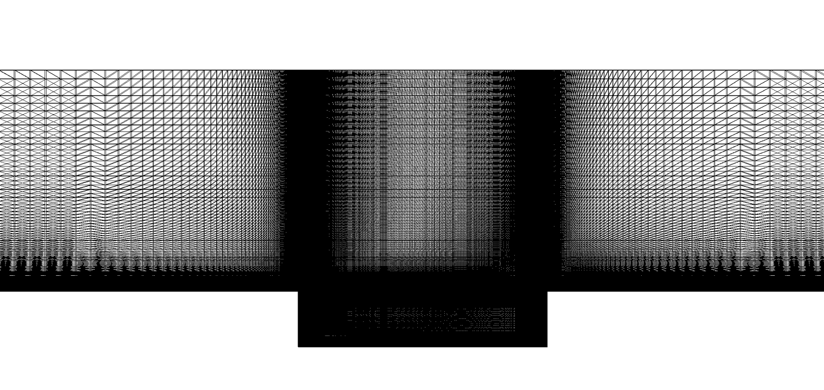
(b) Detail around cavity

Figure 2: Computational mesh: $x-y$ plane cut.

Flow simulations are performed within a time interval $t\in\left[0,T\right]$ with $T=12.5$ time units. We employ the second-order accurate implicit three-point backward differentiation formula, which is a linear multistep scheme characterized by $k=2$, $\alpha_{0}=1$, $\alpha_{1}=-4/3$, $\alpha_{2}=1/3$, $\beta_{0}=2/3$, $\beta_{1}=\beta_{2}=0$, for time integration; future work will perform numerical experiments with Runge–Kutta schemes. The O$\Delta$E (2.3) arising at each time step is solved by a Newton–Krylov method, where GMRES is employed as the iterative linear solver with a restrictive additive Schwarz preconditioner (with no fill in) and the previous 50 Krylov vectors are employed for orthogonalization. Convergence is declared when the residual norm is reduced to a factor of $10^{-3}$ of its starting value. All flow computations are performed in a non-dimensional setting.

The initial condition $\bm{{x}}_{0}$ is provided by first computing a steady-state solution, and using that solution as an initial guess for an unsteady ‘transient’ simulation (which captures the initial transient before the flow reaches a quasi-periodic state) of 7.5 time units. The state at the end of the unsteady transient simulation is then used as the initial condition for the subsequent simulations. The steady-state calculation is characterized by the same parameters as above, except that it employs local time stepping with a maximum CFL number of 100, it uses the first-order implicit backward Euler time integration scheme, it assumes a linear variation of the solution within each control volume, it employs a Spalart–Allmaras turbulence model, and it employs only one Newton iteration per (pseudo) time step.

The output of interest is the pressure at location (0.0001,-0.0508,0.0025), which is shown in the bottom row of Figure 4. All errors are reported as the $\ell^{2}$ relative error in this quantity, i.e.,

$$\varepsilon(p,p_{\star})=\frac{\sqrt{\sum_{n=1}^{T/\Delta t_{\star}}\left(P_{\star}(p)(n\Delta t_{\star})-p_{\star}(n\Delta t_{\star})\right)^{2}}}{\sqrt{\sum_{n=1}^{T/\Delta t}p_{\star}(n\Delta t_{\star})^{2}}},$$

where $p\mathrel{\mathop{\mathchar 58\relax}}\mathbb{N}(T/\Delta t)\rightarrow\mathbb{R}$ is the pressure for the model of interest, $p_{\star}\mathrel{\mathop{\mathchar 58\relax}}\mathbb{N}(T/\Delta t_{\star})\rightarrow\mathbb{R}$ is this pressure response of the designated ‘truth’ model (typically the full-order model), and $P_{\star}$ is a linear interpolation of the pressure response onto the grid based on the truth-model time step $\Delta t_{\star}$.

All computations are performed in double-precision arithmetic on a parallel Linux cluster using 48 cores across 6 nodes.

7.2 Time-step verification

Because this paper considers the time step to be an important parameter in model reduction, we first perform a time-step verification study to ensure we employ an appropriate ‘nominal’ time step. Figure 3 reports these results using a time-step refinement factor of two. A time step of $\Delta t_{\star}=0.0015$ time units yields observed convergence rates in both the instantaneous drag force on the lower wall and instantaneous pressure at $t=T$ that are close to the asymptotic rate of convergence (2.0) of three-point BDF2 scheme. Further, this value also leads to sub-2% errors in both quantities, which we deem to be sufficient for this set of experiments.

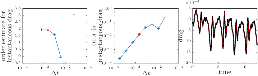
(a) Drag: $\Delta t_{\star}=0.0015$ yields an approximate rate of convergence of 1.94 and an estimated error in the output quantity (computed via Richardson extrapolation) of $1.26\times 10^{-2}$. The red points denote the result for $\Delta t_{\star}=0.0015$. The rightmost plot shows the time-dependent response for the finest tested time step $\Delta t=1.875\times 10^{-4}$ (black solid) and the converged time step $\Delta t_{\star}=0.0015$ (red dashed).

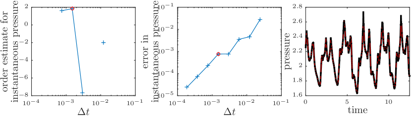
(b) Pressure: $\Delta t_{\star}=0.0015$ yields an approximate rate of convergence of 1.83 and an estimated error in the output quantity (computed via Richardson extrapolation) of $7.68\times 10^{-4}$. The red points denote the result for $\Delta t_{\star}=0.0015$. The rightmost plot shows the time-dependent response for the finest tested time step $\Delta t=1.875\times 10^{-4}$ (black solid) and the converged time step $\Delta t_{\star}=0.0015$ (red dashed).

Figure 3: Time-step verification study. Note that the approximated convergence rates are close to the asymptotic value of 2.0 for the BDF2 scheme.

Figure 4 shows several instantaneous snapshots of the vorticity field and corresponding pressure field generated by the high-fidelity CFD model. The flow within the cavity is quasi-periodic; during one cycle, vorticity is shed from the leading edge of the cavity, convects downstream, and impinges on the aft edge of the cavity. Upon impingement, an acoustic disturbance is generated which propagates upstream and scatters on the leading edge of the cavity, generating a new vortical disturbance to initiate the next oscillation cycle. The pressure fields in the bottom row of Figure 4 reveal regions of low pressure (blue contours) associated with vortices, as well as acoustic disturbances both within the cavity and radiating outside the cavity. This complex flow is governed by the interactions of several nonlinear processes, including roll-up of the shear layer vortices, impingement of the vortices on the aft wall resulting in sound generation, propagation of nonlinear acoustic waves, and interaction of these waves with the shear layer vorticity.

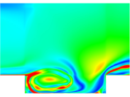
(a) time = 2.10

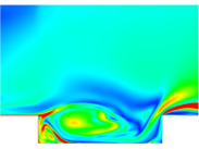
(b) time = 2.61

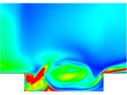
(c) time = 3.12

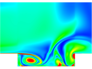
(d) time = 3.63

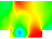
(e) time = 2.10

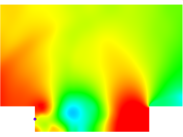
(f) time = 2.61

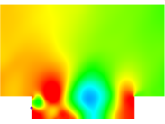
(g) time = 3.12

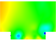
(h) time = 3.63

Figure 4: Instantaneous CFD vorticity field (top) and pressure field (bottom) during one oscillation cycle. The dot on the forward wall of the cavity indicates the location of the pressure signal output.

7.3 Reduced-order models

To construct both the Galerkin and LSPG ROMs, we employ the proper orthogonal decomposition (POD) technique; we employ a constant weighting matrix $\bm{{A}}=\bm{{I}}$ for the LSPG ROM. To construct the POD basis, we set $\bm{{\Phi}}\leftarrow\bm{{\Phi}}\left(\mathcal{X},\nu\right)$, where $\bm{{\Phi}}$ is computed via Algorithm 1 of the appendix with snapshots consisting of the initial-condition-centered full-order model states $\mathcal{X}=\{\bm{{x}}_{\star}(k\Delta t_{\star})-\bm{{x}}_{0}\}_{k=1}^{8334}$, where $\bm{{x}}_{\star}$ denotes the FOM response computed for a time step of $\Delta t_{\star}=0.0015$. Three values of the energy criterion $\nu\in[0,1]$ are used during the experiments: $\nu=1-10^{-4}$ (${p}=204$), $\nu=1-10^{-5}$ (${p}=368$), and $\nu=1-10^{-6}$ (${p}=564$). Figure 5 shows a selection of the energy component of the computed POD modes. Note that as the mode number increases, the modes capture finer spatial-scale behavior, which we expect to be associated with finer time-scale behavior; this will be verified in Section 7.5.1.

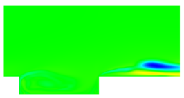
(a) mode 1

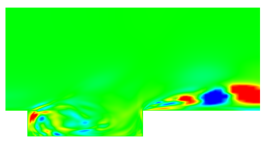
(b) mode 21

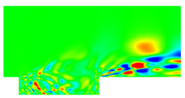
(c) mode 101

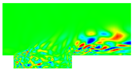
(d) mode 201

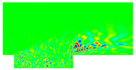
(e) mode 401

Figure 5: Visualization of the energy component of the POD modes.

We first repeat the time-step verification study, but we do so for the reduced-order models (again using the BDF2 scheme) in the time interval $0\leq t\leq 0.55$, as all Galerkin ROMs remain stable in this time interval. Figure 6 reports these results. First, we note that the Galerkin ROM converges an approximated rate of 2.0, which is what we expect given that the Galerkin ROM simply associates with a time-step-independent ODE (3.2). However, the LSPG ROM does not exhibit this behavior; in fact the error convergence is not even monotonic. This is likely due to the fact that the method does not associate with a time-step-independent ODE.

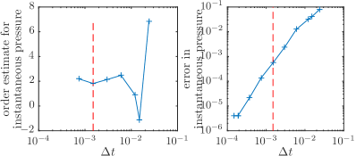
(a) Galerkin reduced-order model

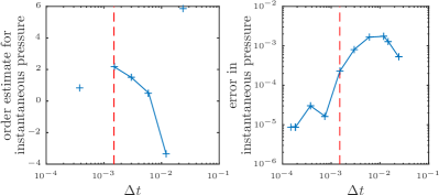
(b) LSPG reduced-order model

Figure 6: Time-step verification study for Galerkin and LSPG reduced-order models for ${p}=368$ and $0\leq t\leq 0.55$. While the approximated convergence rate for the Galerkin reduced-order model is close to the asymptotic value of 2.0 for the BDF2 scheme, this is not observed for the LSPG reduced-order model. Note that the error for each ROM is computed with respect its response for finest Richardson extrapolation, and a dashed red line indicates the snapshot-collection time step $\Delta t_{\star}=0.0015$. See Figure 7(c–d) for the associated time-dependent responses.

We next perform simulations for both reduced-order models for all tested basis dimensions and time steps; Figure 7 reports the time-dependent responses. When a response stops before the end of the time interval, this indicates that a negative pressure was encountered, which causes AERO-F to exit the simulation. We interpret this phenomenon as a non-physical instability.

First, note that the Galerkin ROMs become unstable (i.e., generate a negative pressure) for all time steps and all basis dimensions. This is consistent with previously reported results [20, 21, 19, 18] that indicate Galerkin projection almost always leads to inaccurate responses for compressible fluid-dynamics problems. In contrast, the LSPG ROM results in many stable, accurate responses for all basis dimensions. Further, LSPG responses exhibit a clear dependence on the time step $\Delta t$. Subsequent sections provide a deeper analysis of this dependence.

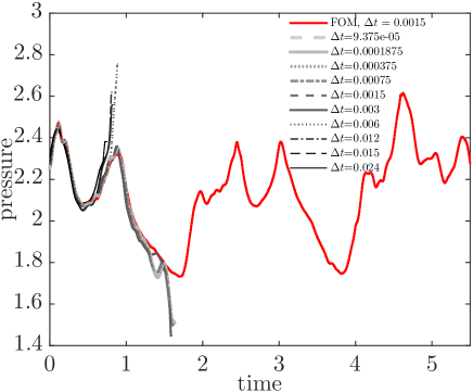
(a) Galerkin, ${p}=204$

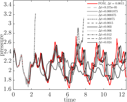
(b) LSPG, ${p}=204$

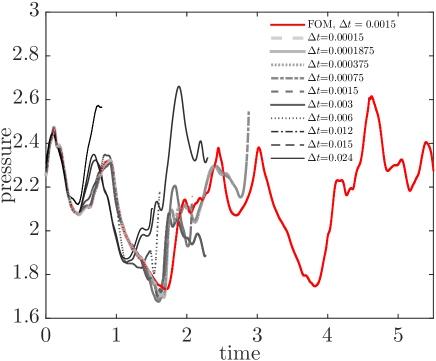
(c) Galerkin, ${p}=368$

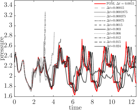
(d) LSPG, ${p}=368$

(e) Galerkin, ${p}=564$

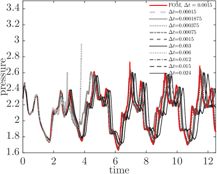
(f) LSPG, ${p}=564$

Figure 7: Responses generated by Galerkin and LSPG ROMs for different basis sizes ${p}$ and time steps $\Delta t$

7.4 Limiting case: comparison

We next compare the responses of the Galerkin and LSPG ROMs for small time windows (when the Galerkin responses remain stable) and small time steps. Figure 8 reports $\varepsilon(p_{\text{discrete~{}opt.}},p_{\text{Gal}_{\star}})$—which is the difference between the pressure responses generated by the LSPG ROM with different time steps and the Galerkin ROM with a fixed time step $\Delta t=1.875\times 10^{-4}$ (the smallest tested time step)—for a time window $0\leq t\leq 1.1$. These responses support an important conclusion (see Theorem 5.3): the Galerkin and LSPG ROMs are equal in the limit of $\Delta t\rightarrow 0$ for $\bm{{A}}=1/\sqrt{\alpha_{0}}\bm{{I}}$, which is what we employ for the LSPG ROM (note that $\alpha_{0}=1$ for this time integrator). This has significant consequences for the LSPG ROM, as decreasing the time step leads to the same unstable response as Galerkin; larger time steps are needed to ensure the LSPG ROM is stable for the entire time interval.

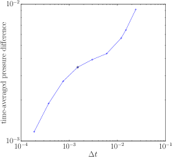
(a) ${p}=204$

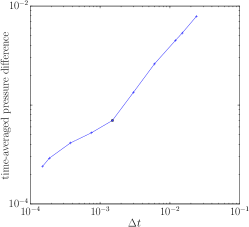
(b) ${p}=368$

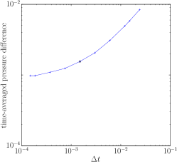
(c) ${p}=564$

Figure 8: Difference $\varepsilon(p_{\text{LSPG}},p_{\text{Gal}_{\star}})$ between the pressure responses generated by the LSPG ROM with different time steps and the Galerkin ROM with a fixed time step $\Delta t=1.875\times 10^{-4}$ in $0\leq t\leq 1.1$. This demonstrates convergence of the LSPG ROM to Galerkin as $\Delta t\rightarrow 0$.

Figure 9 reports $\varepsilon(p_{\text{discrete~{}opt.}},p_{\text{FOM}_{\star}})$ and $\varepsilon(p_{\text{Gal.}},p_{\text{FOM}_{\star}})$—which are the differences between the two ROM-generated pressure responses and the full-order model pressure response for $\Delta t=1.875\times 10^{-4}$—as a function of the time step for all three basis dimensions and three time intervals. These results highlight a critical observation: the LSPG ROM is more accurate for an intermediate time step. This not only supports the result of Corollary 6.17, but provides an interesting insight: taking a larger time step not only leads to better speedups (i.e., the end of the time interval is reached in fewer time steps), but it also decreases the error, sometimes significantly. This is further explored in the next section.

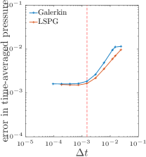
(a) $0\leq t\leq 0.55$, ${p}=204$

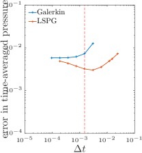
(b) $0\leq t\leq 1.1$, ${p}=204$

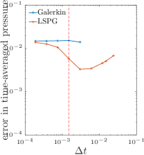
(c) $0\leq t\leq 1.54$, ${p}=204$

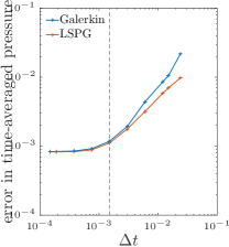
(d) $0\leq t\leq 0.55$, ${p}=368$

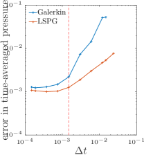
(e) $0\leq t\leq 1.1$, ${p}=368$

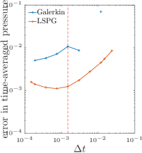
(f) $0\leq t\leq 1.65$, ${p}=368$

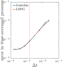
(g) $0\leq t\leq 0.55$, ${p}=564$

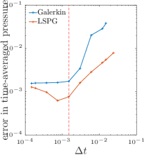
(h) $0\leq t\leq 1.1$, ${p}=564$

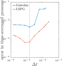
(i) $0\leq t\leq 1.65$, ${p}=564$

Figure 9: Galerkin errors $\varepsilon(p_{\text{Gal.}},p_{\text{FOM}_{\star}})$ and LSPG errors $\varepsilon(p_{\text{LSPG}},p_{\text{FOM}_{\star}})$ over different time intervals, time steps, and basis dimensions. For reference, a dashed red line indicates the snapshot-collection time step $\Delta t_{\star}=0.0015$.

7.5 Time-step selection

Recall from Corollary 6.17 and Remark 6.18 that decreasing the time step $\Delta t$ has a non-obvious effect on the error bound for the LSPG ROM. We now assess these effects for the current problem.

7.5.1 Spectral content of POD basis

In our interpretation of the error bound (6.65) for the LSPG ROM applied to the backward Euler scheme, we noted that the time step should be ‘matched’ to the spectral content of the trial basis $\bm{{\Phi}}$. This is of practical importance, as selecting an appropriate time step for the ROM should take into account the relevant temporal dynamics associated with the basis. For example, a time step may be too small if the basis has filtered out modes with a time scale matching that of the time step. If we assume that the basis $\bm{{\Phi}}$ is computed via POD, then we would expect the vectors to be naturally ordered such that lower mode numbers are associated with lower temporal frequencies. Then, including additional modes has the effect of encoding information at higher frequencies. It follows that the time step should be decreased as additional modes are retained in construction of the ROM.

Here we investigate the validity of this assumption by examining the spectral content of the POD basis vectors for the current cavity-flow problem. We compute the time histories of the generalized coordinates by projecting the FOM solution onto the POD basis as ${{\hat{\bm{{x}}}}_{\star}}(k\Delta t_{\star})\vcentcolon=\bm{{\Phi}}^{T}(\bm{{x}}_{\star}(k\Delta t_{\star})-\bm{{x}}_{0})$, $k\in\mathbb{N}(8334)$. We then compute power spectral densities of the generalized coordinates ${{\hat{\bm{{x}}}}_{\star}}(t)$. Figure 10(a) shows sample spectra, normalized by the total energy in each signal, for several of the POD modes. The figure shows that energy shifts to higher frequencies as the POD mode number increases, confirming our assumption for this example. This is further quantified by calculating a characteristic time-scale $\tau_{95}$ associated with each mode; we define this time scale as the inverse of the frequency below which 95 percent of the energy is captured for that mode. Figure 10(b) plots this time scale versus the mode number, showing a clear trend of decreasing time scale with increasing mode number.

Thus, at least for the present application problem, we expect the optimal time step for the LSPG ROM to decrease as modes are added to the POD basis (this will be verified by Figure 12). Note that systematic calibration could be performed to attempt to automate selection of the ROM time step as a function of basis dimension. While this would be of clear practical interest, we do not pursue it here, as optimal-timestep computation would be complicated in practice by nonlinear interactions arising from the dynamical system, as well as effects from the spatial-discretization error and POD truncation error.

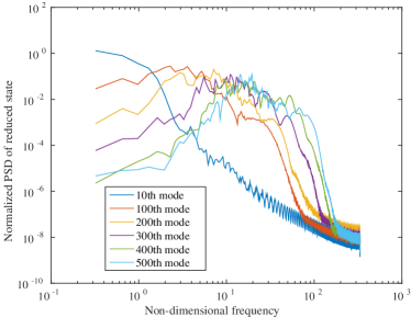
(a) Power spectral densities of several generalized coordinate time series for the cavity-flow problem.

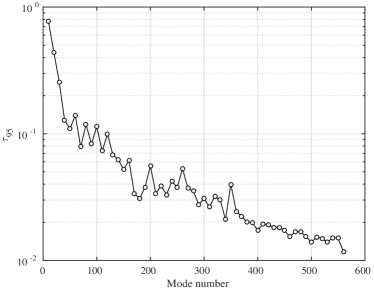
(b) Dependence of the POD mode characteristic time scale on mode number for the cavity-flow problem.

Figure 10: Spectral content of the POD basis.

7.5.2 Error bound behavior

Having verified that higher POD mode numbers correspond to smaller wavelengths, we now numerically assess quantities related to the error bound (6.65). First, Figure 11(a) reports the dependence of the maximum relative projection error $\max_{k}\bar{\mu}_{\star}^{k}(\bm{{\Phi}},\Delta t)$ on the time step $\Delta t$ and the basis dimension, where

$$\bar{\mu}_{\star}^{k}(\bm{{\Phi}},\Delta t)\vcentcolon=\frac{\|(\bm{{I}}-\bm{{\Phi}}\bm{{\Phi}}^{T})(\bm{{x}}_{\star}(k\Delta t)-\bm{{x}}_{\star}((k-1)\Delta t))\|}{\|\bm{{x}}_{\star}(k\Delta t)-\bm{{x}}_{\star}((k-1)\Delta t)\|}.$$

Note that $\bar{\mu}_{\star}^{k}$ is closely related to $\bar{\mu}^{k}$ from error bound (6.65), as they are equal if $\bm{{x}}_{0}+\bm{{\Phi}}{\hat{\bm{{x}}}}_{P}(t)=\bm{{x}}(t)$ and the LSPG ROM computes ${\hat{\bm{{x}}}}_{P}^{k}$ such that $\bar{\mu}^{k}$ is minimized.

These results confirm that adding basis vectors—which we know has the effect of encoding higher frequency content—significantly reduces the projection error for small time steps $\Delta t$, but has less of an effect on larger time steps, as retaining the first POD vectors already enables dynamics at that scale to be captured.

Next, Figure 11(b) plots the error bound (6.65) for a value of $\kappa=1$ and with $\bar{\mu}^{k}=\bar{\mu}_{\star}^{k}$. This highlights an important result: selecting an intermediate time step $\Delta t$ leads to the lowest error bound, regardless of the basis dimension. Even though this result corresponds to the backward Euler integrator, we expect a similar trend to hold for the present experiment, which uses the BDF2 scheme. The next section assesses the performance of the LSPG ROM, including its dependence on the time step.

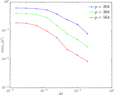
(a) Dependence of the maximum relative projection error $\max_{k}\bar{\mu}_{\star}^{k}$ on the time step $\Delta t$ and basis dimension ${p}$

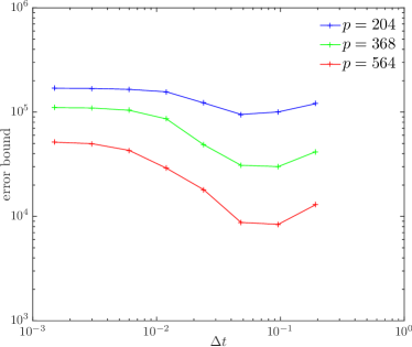
(b) LSPG error bound for the backward Euler scheme (6.65) using experimental data for $\bar{\mu}_{\star}^{k}$ and setting $\kappa=1$ and $\bar{\mu}^{k}=\bar{\mu}_{\star}^{k}$.

Figure 11: Assessment of quantities appearing in error bound (6.65). This analysis suggests that an intermediate time step $\Delta t$ can reduce errors for the LSPG ROM.

7.6 LSPG ROM performance

We now compare the accuracy and walltime performance of the LSPG ROM as the dimension of the basis, time step, and time interval change. The most salient result from Figure 12 is that choosing an intermediate time step leads to both better accuracy and faster simulation times. This shows that our theoretical analysis of the error bound performed in Section 7.5.2 leads to an actual observed performance improvement. For example, consider the ${p}=564$ case over the time interval $0\leq t\leq 2.5$. In this case, a time step of $\Delta t=1.875\times 10^{-4}$ leads to a relative error of $0.0140$ and a simulation time of $289$ hours; increasing this value to $\Delta t=1.5\times 10^{-3}$ reduces the relative error to $9.46\times 10^{-4}$ and the simulation time to $35.8$ hours, which constitutes roughly an order of magnitude improvement in both quantities. Again, this supports the theoretical results of Corollary 6.17 and highlights the critical importance of the time step for LSPG reduced-order models.

In addition, Figure 12 shows that as the basis dimension increases, the optimal time step decreases; this was anticipated from the spectral analysis performed in Section 7.5.1. In addition, adding POD basis vectors does not improve accuracy for large time steps. We interpret this effect as follows: for larger time steps, the first few POD modes accurately capture ‘coarse’ phenomena on the scale of the time step. Therefore, accuracy improvement is not achieved by adding modes that encode dynamics that evolve on a time scale finer than the time step itself.

Further, Figure 12(g) highlights that as the basis dimension increases, the error generally decreases, which is an artifact of the monotonic decrease in the FOM O$\Delta$E residual achieved by the LSPG ROM (Remark 4.1). Finally, the figure shows that as the time interval grows, the optimal time step generally increases.

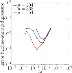
(a) errors for $0\leq t\leq 2.5$

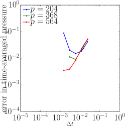
(b) errors for $0\leq t\leq 5.0$

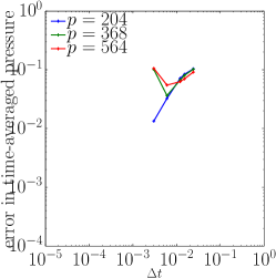
(c) errors for $0\leq t\leq 12.5$

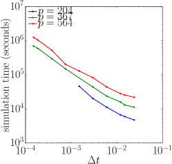
(d) simulation times for $0\leq t\leq 2.5$

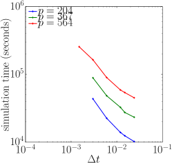
(e) simulation times for $0\leq t\leq 5.0$

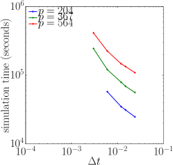
(f) simulation times for $0\leq t\leq 12.5$

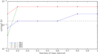
(g) Dependence of optimal time step (in terms of minimizing error) on time interval and basis dimension

Figure 12: Dependence of error and simulation time for the LSPG reduced-order model on the time step $\Delta t$, basis dimension, and time interval

7.7 GNAT: ROM with complexity reduction

In this section, we perform a similar study, but equip the LSPG ROM with complexity reduction in order to achieve computational savings. In particular, we employ the GNAT method [19, 20, 21], which solves Eq. (4.1) with $\bm{{A}}=\left(\bm{{P}}\bm{{\Phi}}_{r}\right)^{+}\bm{{P}}$, where $\bm{{\Phi}}_{r}$ is a basis for the residual and $\bm{{P}}$ consisting of selected rows of the identity matrix.

The problem is identical to that described in Section 7.1 except that we take $T=5.5$ time units and employ a second-order space-accurate dissipation scheme wherein a linear variation of the solution is assumed within each control volume. For this simulation, the full-order model consumes 5.0 hours on 48 cores across six compute nodes.

To construct the trial basis $\bm{{\Phi}}$ and basis for the residual $\bm{{\Phi}}_{r}$ for the GNAT models, we again employ POD. In particular, we set $\bm{{\Phi}}\leftarrow\bm{{\Phi}}\left(\mathcal{X},\nu\right)$, where $\bm{{\Phi}}$ is computed via Algorithm 1 with snapshots consisting of the centered full-order model states $\mathcal{X}=\{\bm{{x}}_{\star}(k\Delta t_{\star})-\bm{{x}}_{0}\}_{k=1}^{3668}$. An energy criterion of $\nu=1-10^{-5}$ (${p}=179$) is used during the experiments. For the residual, we employ $\bm{{\Phi}}_{r}\leftarrow\bm{{\Phi}}\left(\mathcal{X}_{\bm{{r}}},\nu_{\bm{{r}}}\right)$ via Algorithm 1 with snapshots $\mathcal{X}_{\bm{{r}}}=\{{\bm{{r}}}^{n}(\bm{{x}}_{0}+\bm{{\Phi}}\hat{}\bm{{w}}^{n(k)}),\ k\in\mathbb{N}(K(n)),\ n\in\mathbb{N}(2228)\}$ and $\hat{}\bm{{w}}^{n(k)}$ corresponding to the LSPG ROM solution at Gauss–Newton iteration $k$ within time step $n$ using a time step of $\Delta t=6\times 10^{-3}$. Here, $K(n)$ denotes the number of Newton iterations required for convergence of at time instance $n$. An energy criterion of $\nu_{\bm{{r}}}=1.0$ is employed. In addition, the GNAT model sets the Jacobian basis equal to residual basis $\bm{{\Phi}}_{J}=\bm{{\Phi}}_{r}$ and employs $n_{s}=743$ sample nodes that define $\bm{{P}}$, which leads to 4458 rows in $\bm{{P}}$ as there are six conservation equations per node due to the turbulence model (see Ref. [21] for definitions).

The GNAT implementation in AERO-F is characterized by the sample-mesh concept [21]. Figure 13 depicts the sample mesh for this problem, which was constructed using $n_{c}=2228$ working columns [21, Algorithm 3], and includes two layers of nodes around the sample nodes (to enable the residual to be computed at the sample nodes). It is characterized by 7,974 total nodes (4.1% of the original mesh) and 17,070 total volumes (3.0% of the original mesh). Due to the small footprint of the sample mesh, the GNAT simulations are run using only 2 cores on a single compute node.

(a) Full domain

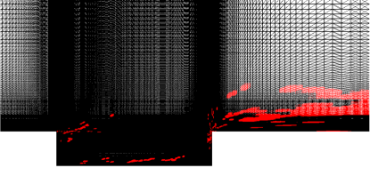
(b) Zoom on cavity

Figure 13: Sample mesh (red) embedded within original mesh. The sample mesh is used to to enable low-computational-footprint simulations with the GNAT reduced-order model.

Figure 14 reports the results obtained with the GNAT ROM using different time steps. Critically, note that the GNAT ROM also exhibits a ‘dip’ in the optimal time step, with a time step of $6.0\times 10^{-3}$ yielding the lowest error. In fact, increasing the time step from $1.5\times 10^{-3}$ to $6.0\times 10^{-3}$ decreases the error from 3.32% to 2.25% and also significantly increases the computational savings relative to the full-order model (as measured in core–hours) from 14.9 to 55.7. This highlights that the analysis is also relevant to ROMs equipped with complexity reduction.

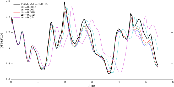
(a) responses

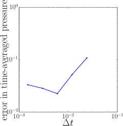
(b) errors

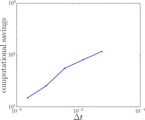
(c) computational savings

Figure 14: Responses, errors $\varepsilon(p_{\text{GNAT}},p_{\text{FOM}_{\star}})$, and computational savings (as measured in core–hours) produced by the GNAT reduced-order model for different time steps $\Delta t$.

7.8 Summary of experimental results

We now briefly summarize the main experimental results:

• Galerkin ROMs are unstable for long time intervals (Figure 7).

• LSPG ROMs are only unstable for small time steps (Figure 7).

• Galerkin and LSPG ROMs are equivalent as $\Delta t\rightarrow 0$ (Figure 8).

• LSPG ROMs are more accurate than Galerkin ROMs over small time windows where Galerkin is stable (Figure 9).

• LSPG ROMs are most accurate for an intermediate time step (Figure 9).

• Adding POD modes has the effect of including higher-frequency response components (Figure 10).

• The theoretical error bound for the LSPG ROM exhibits the same time step ‘dip’ as the experimentally observed error (Figure 11).

• The optimal time step for the LSPG ROM decreases as modes are added to the POD basis (Figure 12).

• Adding modes to the POD basis has little effect on LSPG ROM accuracy for large time steps (Figure 12).

• The optimal time step for the LSPG ROM tends to increase as the time interval increases (Figure 12(g)).

• The GNAT ROM, which is discrete optimal and is equipped with complexity reduction, also produces minimal error for an intermediate time step (Figure 14).

8 Conclusions

This work has performed a comparative theoretical and experimental analysis of Galerkin and LSPG reduced-order models for linear multistep schemes and Runge–Kutta schemes. We have demonstrated a number of new findings that have important practical implications, including conditions under which the LSPG ROM has a time-continuous representation, conditions under which the two techniques are equivalent, and time-discrete error bounds for the two approaches.

Perhaps most surprisingly, we demonstrated that decreasing the time step does not necessarily decrease the error for the LSPG ROM. This phenomenon arose in both the theoretical analysis and in numerical experiments. In particular, our results suggest that the time step should be ‘matched’ to the spectral content of the reduced basis. In the experiments, we showed that increasing the time step to an intermediate value decreased both the error and the simulation time by an order of magnitude in certain cases. Alternatively, decreasing the time step cause the LSPG ROM to become unstable for longer time intervals. This highlights the critical importance of time-step selection for LSPG ROMs.

Appendix

Algorithm 1 reports the algorithm for computing a POD basis using normalized snapshots.

0:  Set of snapshots $\mathcal{X}\equiv\{{\bm{w}}_{i}\}_{i=1}^{n_{w}}\subset\mathbb{R}^{N}$, energy criterion $\nu\in[0,1]$

0:  $\bm{{\Phi}}\left(\mathcal{X},\nu\right)$

1:   Compute thin singular value decomposition $\bm{W}=\bm{U}\bm{\Sigma}\bm{V}^{T}$, where $\bm{W}\equiv\left[{\bm{w}}_{1}/\|{\bm{w}}_{1}\|\ \cdots\ {\bm{w}}_{n_{\bm{w}}}/\|{\bm{w}}_{n_{\bm{w}}}\|\right]$.

2:  Choose dimension of truncated basis ${p}=n_{e}(\nu)$, where

$$n_{e}(\nu) =\arg\min_{i\in\mathcal{V}(\nu)}i$$

$$\mathcal{V}(\nu) \vcentcolon=\{n\in\mathbb{N}({n_{w}})\ |\ \sum_{i=1}^{n}\sigma_{i}^{2}/\sum_{i=1}^{{n_{w}}}\sigma_{i}^{2}\geq\nu\},$$

and $\bm{\Sigma}\equiv\text{diag}\left(\sigma_{i}\right)$.

3:  $\bm{{\Phi}}\left(\mathcal{X},\nu\right)=\left[\bm{u}^{1}\ \cdots\ \bm{u}^{{p}}\right]$, where $\bm{U}\equiv\left[\bm{u}^{1}\ \cdots\ \bm{u}^{{n_{w}}}\right]$.

Algorithm 1 Proper-orthogonal-decomposition basis computation (normalized snapshots)

References

• [1] R. Abgrall and D. Amsallem, Robust model reduction by $l^{1}$-norm minimization and approximation via dictionaries: application to linear and nonlinear hyperbolic problems, Stanford University Preprint, (2015).
• [2] R. Alexander, Diagonally implicit runge-kutta methods for stiff ODE’s, SIAM Journal on Numerical Analysis, 14 (1977), pp. 1006–1021.
• [3] D. Amsallem, M. Zahr, and K. Washabaugh, Fast local reduced basis updates for the efficient reduction of nonlinear systems with hyper-reduction, Advances in Computational Mathematics, Special Issue on Model Reduction of Parameterized Systems (2015).
• [4] S. An, T. Kim, and D. James, Optimizing cubature for efficient integration of subspace deformations, ACM Transactions on Graphics (TOG), 27 (2008), p. 165.
• [5] H. Antil, S. Field, F. Herrmann, R. Nochetto, and M. Tiglio, Two-step greedy algorithm for reduced order quadratures, Journal of Scientific Computing, 57 (2013), pp. 604–637.
• [6] H. Antil, M. Heinkenschloss, and D. C. Sorensen, Application of the discrete empirical interpolation method to reduced order modeling of nonlinear and parametric systems, vol. 8 of Springer MS&A series: Reduced Order Methods for modeling and computational r G. Rozza, Eds, Springer-Verlag Italia, Milano, 2013.
• [7] P. Astrid, S. Weiland, K. Willcox, and T. Backx, Missing point estimation in models described by proper orthogonal decomposition, IEEE Transactions on Automatic Control, 53 (2008), pp. 2237–2251.
• [8] N. Aubry, P. Holmes, J. L. Lumley, and E. Stone, The dynamics of coherent structures in the wall region of a turbulent boundary layer, Journal of Fluid Mechanics, 192 (1988), pp. 115–173.
• [9] M. Balajewicz and E. Dowell, Stabilization of projection-based reduced order models of the navier–stokes equations, Nonlinear Dynamics, 70 (2012), pp. 1619–1632.
• [10] M. Balajewicz, E. Dowell, and B. Noack, Low-dimensional modelling of high-reynolds-number shear flows incorporating constraints from the navier–stokes equation, Journal of Fluid Mechanics, 729 (2013), pp. 285–308.
• [11] M. F. Barone, I. Kalashnikova, D. J. Segalman, and H. K. Thornquist, Stable Galerkin reduced order models for linearized compressible flow, Journal of Computational Physics, 228 (2009), pp. 1932–1946.
• [12] M. Barrault, Y. Maday, N. C. Nguyen, and A. T. Patera, An ‘empirical interpolation’ method: application to efficient reduced-basis discretization of partial differential equations, Comptes Rendus Mathématique Académie des Sciences, 339 (2004), pp. 667–672.
• [13] P. Benner, S. Gugercin, and K. Willcox, A survey of model reduction methods for parametric systems, SIAM Review, 57 (2015), pp. 483–531.
• [14] M. Bergmann, C.-H. Bruneau, and A. Iollo, Enablers for robust pod models, Journal of Computational Physics, 228 (2009), pp. 516 – 538.
• [15] L. Blackford, A. Cleary, J. Choi, E. d’Azevedo, J. Demmel, I. Dhillon, J. Dongarra, S. Hammarling, G. Henry, A. Petitet, et al., ScaLAPACK Users’ Guide, Society for Industrial and Applied Mathematics, 1997.
• [16] R. Bos, X. Bombois, and P. Van den Hof, Accelerating large-scale non-linear models for monitoring and control using spatial and temporal correlations, Proceedings of the American Control Conference, 4 (2004), pp. 3705–3710.
• [17] T. Bui-Thanh, K. Willcox, and O. Ghattas, Model reduction for large-scale systems with high-dimensional parametric input space, SIAM Journal on Scientific Computing, 30 (2008), pp. 3270–3288.
• [18] K. Carlberg, Model reduction of nonlinear mechanical systems via optimal projection and tensor approximation, PhD thesis, Stanford University, August 2011.
• [19] K. Carlberg, C. Bou-Mosleh, and C. Farhat, Efficient non-linear model reduction via a least-squares Petrov–Galerkin projection and compressive tensor approximations, International Journal for Numerical Methods in Engineering, 86 (2011), pp. 155–181.
• [20] K. Carlberg, J. Cortial, D. Amsallem, M. Zahr, and C. Farhat, The GNAT nonlinear model reduction method and its application to fluid dynamics problems, AIAA Paper 2011-3112, 6th AIAA Theoretical Fluid Mechanics Conference, Honolulu, HI, (2011).
• [21] K. Carlberg, C. Farhat, J. Cortial, and D. Amsallem, The GNAT method for nonlinear model reduction: effective implementation and application to computational fluid dynamics and turbulent flows, Journal of Computational Physics, 242 (2013), pp. 623–647.
• [22] K. Carlberg, R. Tuminaro, and P. Boggs, Efficient structure-preserving model reduction for nonlinear mechanical systems with application to structural dynamics, in AIAA Paper 2012-1969, 53rd AIAA/ASME/ASCE/AHS/ASC Structures, Structural Dynamics and Materials Conference, Honolulu, Hawaii, April 23–26 2012.
• [23] K. Carlberg, R. Tuminaro, and P. Boggs, Preserving Lagrangian structure in nonlinear model reduction with application to structural dynamics, SIAM J. Sci. Comput., 37 (2015), pp. B153—B184.
• [24] S. Chaturantabut and D. C. Sorensen, Nonlinear model reduction via discrete empirical interpolation, SIAM Journal on Scientific Computing, 32 (2010), pp. 2737–2764.
• [25] P. Constantine and Q. Wang, Residual minimizing model reduction for parameterized nonlinear dynamical systems, SIAM J. Sci. Comput., 34 (2012), pp. A2118–A2144.
• [26] M. Drohmann, B. Haasdonk, and M. Ohlberger, Reduced basis approximation for nonlinear parametrized evolution equations based on empirical operator interpolation, SIAM Journal on Scientific Computing, 34 (2012), pp. A937–A969.
• [27] R. Everson and L. Sirovich, Karhunen–Loève procedure for gappy data, Journal of the Optical Society of America A, 12 (1995), pp. 1657–1664.
• [28] F. Fang, C. Pain, I. Navon, A. Elsheikh, J. Du, and D. Xiao, Non-linear Petrov–Galerkin methods for reduced order hyperbolic equations and discontinuous finite element methods, Journal of Computational Physics, 234 (2013), pp. 540 – 559.
• [29] C. Farhat, P. Avery, T. Chapman, and J. Cortial, Dimensional reduction of nonlinear finite element dynamic models with finite rotations and energy-based mesh sampling and weighting for computational efficiency, International Journal for Numerical Methods in Engineering, 98 (2014), pp. 625–662.
• [30] C. Farhat, P. Geuzaine, and G. Brown, Application of a three-field nonlinear fluid-structure formulation to the prediction of the aeroelastic parameters of an F-16 fighter, Computers & Fluids, 32 (2003), pp. 3–29.
• [31] C. Foias, M. Jolly, I. Kevrekidis, and E. Titi, Dissipativity of numerical schemes, Nonlinearity, 4 (1991), p. 591.
• [32] D. Galbally, K. Fidkowski, K. Willcox, and O. Ghattas, Non-linear model reduction for uncertainty quantification in large-scale inverse problems, International Journal for Numerical Methods in Engineering, 81 (2009), pp. 1581–1608.
• [33] B. Galletti, C. Bruneau, L. Zannetti, and A. Iollo, Low-order modelling of laminar flow regimes past a confined square cylinder, Journal of Fluid Mechanics, 503 (2004), pp. 161–170.
• [34] P. Geuzaine, G. Brown, C. Harris, and C. Farhat, Aeroelastic dynamic analysis of a full F-16 configuration for various flight conditions, AIAA Journal, 41 (2003), pp. 363–371.
• [35] P. Holmes, J. Lumley, and G. Berkooz, Turbulence, Coherent Structures, Dynamical Systems and Symmetry, Cambridge University Press, 1996.
• [36] A. Iollo, S. Lanteri, and J. A. Desideri, Stability properties of POD–Galerkin approximations for the compressible Navier–Stokes equations, Theoretical and Computational Fluid Dynamics, 13 (2000), pp. 377–396.
• [37] M. Jolly, I. Kevrekidis, and E. Titi, Preserving dissipation in approximate inertial forms for the Kuramoto-Sivashinsky equation, Journal of Dynamics and Differential Equations, 3 (1991), pp. 179–197.
• [38] I. Kalashnikova and M. Barone, On the stability and convergence of a Galerkin reduced order model (rom) of compressible flow with solid wall and far-field boundary treatment, International Journal for Numerical Methods in Engineering, 83 (2010), pp. 1345–1375.
• [39] S. Lall, P. Krysl, and J. Marsden, Structure-preserving model reduction for mechanical systems, Physica D: Nonlinear Phenomena, 184 (2003), pp. 304–318.
• [40] P. A. LeGresley, Application of proper orthogonal decomposition (POD) to design decomposition methods, PhD thesis, Stanford University, 2006.
• [41] M. Marion and R. Temam, Nonlinear Galerkin methods, SIAM Journal on Numerical Analysis, 26 (1989), pp. 1139–1157.
• [42] N. Ngoc Cuong, K. Veroy, and A. T. Patera, Certified real-time solution of parametrized partial differential equations, in Handbook of Materials Modeling, S. Yip, ed., Springer Netherlands, 2005, pp. 1529–1564.
• [43] B. R. Noack, P. Papas, and P. A. Monkewitz, The need for a pressure-term representation in empirical Galerkin models of incompressible shear flows, Journal of Fluid Mechanics, 523 (2005), pp. 339–365.
• [44] C. Prud’homme, D. V. Rovas, K. Veroy, L. Machiels, Y. Maday, A. T. Patera, and G. Turinici, Reliable real-time solution of parameterized partial differential equations: Reduced-basis output bound methods, Journal of Fluids Engineering, 124 (2002), pp. 70–80.
• [45] M. Rathinam and L. R. Petzold, A new look at proper orthogonal decomposition, SIAM Journal on Numerical Analysis, 41 (2003), pp. 1893–1925.
• [46] D. Rempfer, On low-dimensional Galerkin models for fluid flow, Theoretical and Computational Fluid Dynamics, 14 (2000), pp. 75–88.
• [47] C. W. Rowley, T. Colonius, and R. M. Murray, Model reduction for compressible flows using POD and Galerkin projection, Physica D: Nonlinear Phenomena, 189 (2004), pp. 115–129.
• [48] G. Rozza, D. B. P. Huynh, and A. T. Patera, Reduced basis approximation and a posteriori error estimation for affinely parametrized elliptic coercive partial differential equations, Archives of Computational Methods in Engineering, 15 (2008), pp. 229–275.
• [49] D. Ryckelynck, A priori hyperreduction method: an adaptive approach, Journal of Computational Physics, 202 (2005), pp. 346–366.
• [50] O. San and T. Iliescu, Proper orthogonal decomposition closure models for fluid flows: Burgers equation, arXiv preprint arXiv:1308.3276, (2013).
• [51] J. Shen, Long time stability and convergence for fully discrete nonlinear Galerkin methods, Applicable Analysis, 38 (1990), pp. 201–229.
• [52] S. Sirisup and G. Karniadakis, A spectral viscosity method for correcting the long-term behavior of POD models, Journal of Computational Physics, 194 (2004), pp. 92–116.
• [53] L. Sirovich, Turbulence and the dynamics of coherent structures. III: dynamics and scaling, Quarterly of Applied Mathematics, 45 (1987), pp. 583–590.
• [54] P. Spalart and S. Allmaras, A one-equation turbulence model for aerodynamic flows, La Recherche Aérospatiale, 1 (1994), p. 5.
• [55] K. Veroy and A. T. Patera, Certified real-time solution of the parametrized steady incompressible Navier–Stokes equations: Rigorous reduced-basis a posteriori error bounds, International Journal for Numerical Methods in Fluids, 47 (2005), pp. 773–788.
• [56] K. Veroy, C. Prud’homme, D. V. Rovas, and A. T. Patera, A posteriori error bounds for reduced-basis approximation of parametrized noncoercive and nonlinear elliptic partial differential equations, AIAA Paper 2003-3847, 16th AIAA Computational Fluid Dynamics Conference, Orlando, FL, (2003).
• [57] Z. Wang, I. Akhtar, J. Borggaard, and T. Iliescu, Proper orthogonal decomposition closure models for turbulent flows: a numerical comparison, Computer Methods in Applied Mechanics and Engineering, 237 (2012), pp. 10–26.