Statefinder diagnosis for holographic dark energy in the DGP braneworld

Abstract

Many dark energy (DE) models have been proposed, in recent years, to explain acceleration of the Universe expansion. It seems necessary to discriminate the various DE models in order to check the viability of each model. Statefinder diagnostic is a useful method which can differentiate various DE models. In this paper, we investigate the statefinder diagnosis parameters for the holographic dark energy (HDE) model in two cosmological setup. First, we study statefinder diagnosis for HDE in the context of flat Friedmann-Robertson-Walker (FRW) Universe in Einstein gravity. Then, we extend our study to the DGP braneworld framework. As system’s IR cutoff we chose the Hubble radius and the Granda-Oliveros cutoff inspired by Ricci scalar curvature. We plot the evolution of statefinder parameres $\{r,s\}$ in terms of the redshift parameter $z$. We also compare the results with those obtained for statefinder diagnosis parameters of other DE models, in particular with $\Lambda$CDM model.

I Introduction

Recent astronomical observations such as type Ia supernovae (SNIa) Riess , large scale structure (LSS) COL2001 , and the cosmic microwave background (CMB) anisotropies HAN2000 confirm that our Universe is currently undergoing a phase of accelerated expansion. DE which is responsible for this acceleration has anti-gravity nature and hence push the Universe to accelerate. Although the nature of such a DE is still unknown, many candidates have been proposed for DE in the literatures. The first and simplest candidate for DE is the cosmological constant with equation of state (EoS) parameter $\omega=-1$. But unfortunately, it suffers from some serious problems such as fine-tuning and coincidence problems. A comprehensive but incomplete list of DE scenarios include scalar fields (such as quintessence Wetterich , phantom (ghost) field Caldwell , K-essence Chiba ), the DE models including Chaplygin gas Kamenshchik , agegraphic DE models Cai1 ; Shey2 , HDE model Cohen1 ; Hsu ; Li ; pav1 ; Shey1 and so on.

The HDE model, which has got a lot of attentions in recent years, is based on Cohen et al. Cohen1 works who discussed that in quantum field theory a short distance cutoff could be related to a long distance cutoff (IR cutoff) due to the limit set by black hole formation. If the quantum zero-point energy density is due to a short distance cutoff, then the total energy in a region of size $L$ should not exceed the mass of a black hole of the same size, namely $L^{3}\rho_{D}\leq LM_{p}^{2}$. The largest $L$ is the one saturating this inequality and therefore we obtain the HDE density as Cohen1

$$\rho_{D}=3c^{2}M_{p}^{2}L^{-2},$$ (1)

where $c$ is a numerical constant and $M^{2}_{p}=8\pi G$ is the reduced Planck mass. In the literatures, various IR cutoffs have been considered, which lead to various models of HDE Horava ; Fischler ; Nojiri ; Gao . Recently, Granda and Oliveros (GO) have proposed a new IR cutoff which includes time derivative of the Hubble parameter and is the formal generalization of the Ricci scalar curvature, $L=(\alpha\dot{H}+\beta H^{2})^{-1/2}$ Granda . The advantages of GO cutoff is that the presence of the event horizon is not presumed in this model, so that the causality problem can be avoided Granda . Besides, the fine tuning problem can be solved in this model Granda .

On the other hand, the expansion rate of the Universe is explained by the Hubble parameter $H=\dot{a}/a$, where $a=a(t)$ is the scale factor of the Universe, while the rate of the acceleration or deceleration of the Universe expansion is described by the deceleration parameter,

$$q=-\frac{a\ddot{a}}{\dot{a}^{2}}=-\frac{\ddot{a}}{aH^{2}}.$$ (2)

However, the Hubble parameter $H$ and the deceleration parameter $q$ cannot discriminate various DE models since all DE models leads to $H>0$ and $\ddot{a}>0$ or $q<0$. In addition, the remarkable increase in the accuracy of cosmological observational data during the last few years, compel us to advance beyond these two important quantities. A question then arise: how can we discriminate and classify various models of DE? In order to answer this question, Sahni, et. al., Sahni and Alam, et al., Alam , proposed a new geometrical diagnostic pair for DE. This diagnostic is constructed from scale factor $a(t)$ and its derivatives up to the third order. The statefinder pair $\{r,s\}$ is defined as Sahni

$$r=\frac{\dddot{a}}{aH^{3}},~{}~{}~{}~{}~{}~{}~{}~{}~{}~{}~{}~{}~{}~{}s=\frac{r-1}{3(q-1/2)}.$$ (3)

The statefinder pair is a geometrical diagnostic in the sense that it is constructed from a spacetime metric directly, and it is more universal than physical variables which depend on the properties of physical fields describing DE, because physical variables are, of course, model-dependent. Usually one can plot the trajectories in the $r-s$ plane corresponding to different DE models to see the qualitatively different behaviors of them. For flat $\Lambda$CDM scenario the statefinder pair is $\{r,s\}=\{1,0\}$ Feng . This fixed point provides a good way of establishing the distance of any given DE model from $\Lambda$CDM model. It was shown that the statefinder pair $\{r,s\}$ can also be related to the EoS parameter of DE and its first time derivative Sahni . The statefinder pair is calculated for a number of existing models of DE having both constant and variable EoS parameter. It was argued that the statefinder can successfully differentiate between a wide variety of DE models including the cosmological constant, quintessence, the Chaplygin gas and interacting DE models (see state ; state1 and references therein). In this paper we would like to study the statefinder pair parameters $\{r,s\}$ for HDE in standard cosmology as well as DGP braneworld scenario.

This paper is outlined as follows. In the next section we investigate statefinder for HDE in standard cosmology with considering Hubble radius and GO cutoff as systems’s IR cutoffs. We also plot the related figures which show the evolution of statefinder in each case. In section III, we extended our study to DGP braneworld and calculate statefinder pair $\{r,s\}$ for HDE in a flat FRW Universe on the brane. The last section is devoted to conclusions and discussions.

II HDE in standard cosmology

Consider a homogeneous and isotropic FRW which has the following metric

$${\rm d}s^{2}=-{\rm d}t^{2}+a^{2}(t)\left(\frac{{\rm d}r^{2}}{1-kr^{2}}+r^{2}{\rm d}\Omega^{2}\right),$$ (4)

where $k=0,1,-1$ represent a flat, closed and open FRW Universe, respectively. Due to the fact that the density of baryonic matter is much smaller than the energy densities of DM and DE, we ignore the baryonic matter throughout the paper. Thus, Friedmann equation in spatially flat FRW Universe may be written as

$$H^{2}=\frac{1}{3M_{p}^{2}}(\rho_{m}+\rho_{D}),$$ (5)

where $\rho_{m}$ and $\rho_{D}$ are the energy densities of DM and DE, respectively. From equation (5) we can write

$$\Omega_{m}+\Omega_{D}=1.$$ (6)

where we have used the following dimensionless energy densities definitions,

$$\Omega_{m}=\frac{\rho_{m}}{3M_{p}^{2}H^{2}},~{}~{}~{}~{}~{}~{}~{}~{}~{}~{}~{}~{}~{}~{}~{}~{}\Omega_{D}=\frac{\rho_{D}}{3M_{p}^{2}H^{2}}.$$ (7)

Recent observational evidences provided by the galaxy clusters supports the interaction between DE and DM Bertolami . In this case, the energy densities of DE and DM no longer satisfy independent conservation laws. They obey instead

$$\dot{\rho}_{m}+3H\rho_{m}=Q,$$ (8)

$$\dot{\rho}_{D}+3H(1+\omega_{D})\rho_{D}=-Q,$$ (9)

where $\omega_{D}=p_{D}/\rho_{D}$ is the EoS parameter of HDE and $Q$ describes the interaction between DE and DM. The choice of the interaction between both components was to get a scaling solution to the coincidence problem such that the Universe approaches a stationary stage in which the ratio of DE and DM becomes a constant Hu . Here, we choose $Q=3b^{2}H(\rho_{D}+\rho_{m})$ as an interaction term with $b^{2}$ being a coupling constant. This expression for the interaction term was first introduced in the study of the suitable coupling between a quintessence scalar field and a pressureless cold DM field Amendola ; Zimdahl .

First, we choose Hubble radius as IR cutoff, $L=H^{-1}$, thus the the hologeraphic energy density reads

$$\rho_{D}=3c^{2}M_{p}^{2}H^{2}.$$ (10)

If we consider $c$ as a constant, then from definition (7) the dimensionless DE density becomes a constant, namely $\Omega_{D}=c^{2}$. In this case, without interaction between DE and DM the accelerated expansion of the Universe cannot be achieved and we get a wrong EoS, namely that for dust, $\omega_{D}=0$ Li . However, as soon as the interaction between two dark component is taken into account, the accelerated expansion can be achieved and implies a constant ratio of the energy densities of both components, thus solving the coincidence problem pav1 .

Taking the time derivative of the Friedmann equation (5) and using Eqs. (6)-(9), we get

$$\frac{\dot{H}}{H^{2}}=-\frac{3}{2}\Big{(}1+\omega_{D}\Omega_{D}\Big{)}.$$ (11)

Also, if we take derivative of Eq. (10) with respect to time, after combining the result with (9) and (11), we obtain the EoS parameter as

$$\omega_{D}=-\frac{b^{2}}{c^{2}(1-c^{2})}.$$ (12)

The rate of deceleration/acceleration of the Universe expansion is characterized by the deceleration parameter that encoded the second derivative of the scale factor. In our case the deceleration parameter is found to be

$$q=-1-\frac{\dot{H}}{H^{2}}=\frac{1}{2}-\frac{3b^{2}}{2(1-c^{2})}.$$ (13)

It is clear that in the absence of the interaction where $b^{2}=0$, we have $w_{D}=0$ and $q=1/2>0$, which implies that we encounter a decelerated Universe. Furthermore, in order to find more sensitive discriminator of the expansion rate, we consider the statefinder parameters which contain the third derivative of the scale factor. The satefinder parameter $r$ can also be expressed as

$$r=1+3\frac{\dot{H}}{H^{2}}+\frac{\ddot{H}}{H^{3}}.$$ (14)

Taking the time derivative of both sides Eq. (5) and using Eqs. (3), (8)-(14), we can obtain the statefinder pair $\{r,s\}$ as

$$r = 1+\frac{9b^{2}(c^{2}+b^{2}-1)}{2(1-c^{2})^{2}},$$ (15)

$$s = \frac{c^{2}+b^{2}-1}{c^{2}-1}.$$ (16)

The statefinder pair parameters $\{r,s\}$ become constant depending on $b^{2}$ and $c^{2}$ parameters. For $c^{2}=1-b^{2}$ we have $\{r,s\}=\{1,0\}$, which is exactly the result obtained for spatially flat $\Lambda$CDM model Feng . So we can find relationship between the coupling constant $b^{2}$ and HDE constant parameter $c^{2}$.

Next, we consider the GO cutoff as the system’s IR cutoff, namely $L=(\alpha\dot{H}+\beta H^{2})^{-1/2}$. This cutoff was first introduced by Granda and Oliveros Granda and can be considered as the formal generalization of the Ricci scalar curvature radius Gao . The cosmological implications of the HDE model with GO cutoff have been investigated in GO . With this IR cutoff, the energy density (1) is written

$$\rho_{D}=3M_{p}^{2}(\alpha H^{2}+\beta\dot{H}),$$ (17)

where $\alpha$ and $\beta$ are constants which should be constrained by observational data, and we have absorbed the constant $c^{2}$ in $\alpha$ and $\beta$ in HDE density. For the case of GO cutoff, we do not need to take into account the interaction between DE and DM and without it we still have acceleration. Thus, for economical reason, here we consider the noninteracting case with $b^{2}=0=Q$, so the continuity equations read to

$$\dot{\rho}_{m}+3H\rho_{m}=0,$$ (18)

$$\dot{\rho}_{D}+3H(1+\omega_{D})\rho_{D}=0.$$ (19)

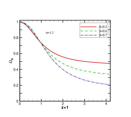
Figure 1: The evolution of $\Omega_{D}$ versus redshift parameter $z$ for HDE with GO cutoff in standard cosmology. Left panel corresponds to $\alpha<1$ and the right panel shows the case $\alpha>1$.

Now taking the time derivative of both sides of Eq. (5) and using Eq. (6), we get

$$\frac{\dot{\rho}_{D}}{3M_{p}^{2}H^{3}}=\frac{2\dot{H}}{H^{2}}+3(1-\Omega_{D}).$$ (20)

From Eq. (17) one can obtain

$$\frac{\dot{H}}{H^{2}}=\frac{\Omega_{D}-\alpha}{\beta}.$$ (21)

The equation of motion for the dimensionless HDE density is obtained by taking the time derivative of relation (7)

$$\dot{\Omega}_{D}=\frac{\dot{\rho}_{D}}{3M_{p}^{2}H^{2}}-2\Omega_{D}\frac{\dot{H}}{H}.$$ (22)

Combining Eqs. (20) and (21) with (22), we arrive at

$${\Omega}^{\prime}_{D}=(1-\Omega_{D})\left[3+\frac{2}{\beta}(\Omega_{D}-\alpha)\right].$$ (23)

where a prime denotes derivative with respect to $x=\ln a$ and we have used relation $\dot{\Omega}_{D}=H{\Omega}^{\prime}_{D}$. The evolution of the dimensionless HDE density $\Omega_{D}$ in terms of redshift parameter $1+z=a^{-1}$ is shown in Fig. (1). From these figures we see that at the early time $\Omega_{D}\rightarrow 0$, while at the late time where $a\rightarrow\infty$, the DE dominated, namely $\Omega_{D}\rightarrow 1$.

Combining Eqs. (17), (20) and (21) with (19), we can obtain the EoS parameter as

$$\omega_{D}=-\frac{1}{\Omega_{D}}\left[1+\frac{2}{3}\left(\frac{\Omega_{D}-\alpha}{\beta}\right)\right]$$ (24)

The deceleration parameter can be expressed in this model as

$$q=-1-\frac{\dot{H}}{H^{2}}=-1-\frac{\Omega_{D}-\alpha}{\beta}.$$ (25)

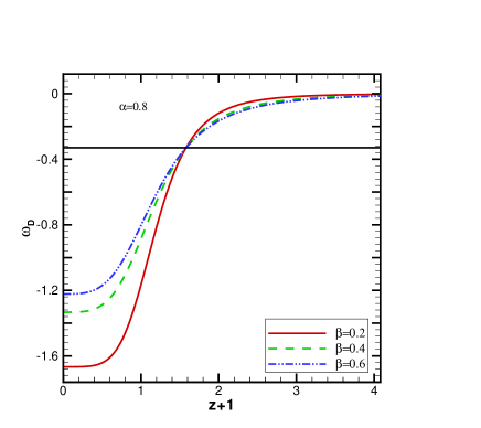
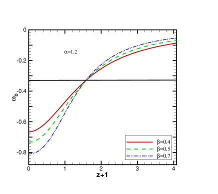
Figure 2: The evolution of $\omega_{D}$ versus redshift parameter $z$ for HDE with GO cutoff in standard cosmology. Left panel corresponds to $\alpha<1$ and the right panel shows the case $\alpha>1$.

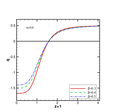
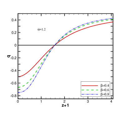
Figure 3: The evolution of the deceleration parameter $q$ against redshift parameter $z$ for HDE with GO cutoff in standard cosmology.

When $\Omega_{D}\rightarrow\alpha=1$ we have $\omega_{D}=-1$ and $q=-1$, similar to the cosmological constant. Therefore, we investigate the behavior of $\omega_{D}$ for values close to $\alpha=1$. We consider the case with $\alpha<1$ and $\alpha>1$ separately. We find that for both cases, our Universe has a transition from deceleration to the acceleration phase around $z\approx 0.6$. The behavior of $\omega_{D}$ and $q$ are plotted in figures 2 and 3. From these figures we see that for $\alpha<1$ the EoS parameter can cross the phantom line in the future, i.e., $\omega_{D}<-1$, while for $\alpha>1$ the EoS parameter is always larger than $-1$.
Taking the time derivative of Eq. (21), after using (23), we obtain

$$\frac{\ddot{H}}{H^{3}}=\frac{2}{\beta^{2}}(\Omega_{D}-\alpha)(1-\alpha)+\frac{3}{\beta}(1-\Omega_{D}).$$ (26)

Inserting Eqs. (21) and (26) in (14), after some calculations, we obtain statefinder pair parameters $\{r,s\}$ as follow,

$$r = 1+\frac{(1-\alpha)}{\beta}\left[3+\frac{2}{\beta}\left(\Omega_{D}-\alpha\right)\right],$$ (27)

$$s = \frac{\alpha-1}{6\beta}.$$ (28)

It can be easily seen that for $\alpha=1$, we have $\{r=1,s=0\}$ as expected. The statefinder parameter $r(z)$ is plotted in figure 4 and 5 for two cases. These results are compatible with the arguments given in Alam ; Sahni .

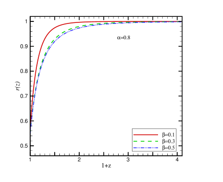
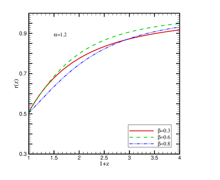
Figure 4: The evolution of the statefinder parameter $r$ versus redshift parameter $z$ for $\alpha<1$ (left panel) and $\alpha>1$ (right panel).

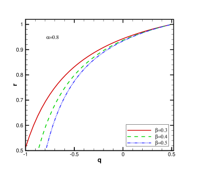
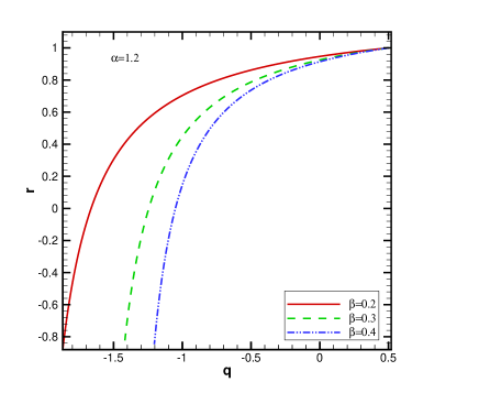
Figure 5: The evolution of the statefinder parameter $r$ versus declaration parameter $q$ for $\alpha<1$ (left panel) and $\alpha>1$ (right panel).

III DGP bareworld model

In this section, we would like to extend the study to braneworld scenario. According to this scenario, our Universe is realized as a 3-brane embedded in a five dimensional spacetime. A special version of braneworld scenario was proposed by Dvali- Gabadadze-Porrati (DGP) Dvali , in which our four-dimensional FRW Universe embedded in a five-dimensional Minkowski bulk with infinite size. The recovery of the usual gravitational laws in this picture is obtained by adding to the action of the brane an Einstein-Hilbert term computed with the brane intrinsic curvature. The presence of such a term in the action is generically induced by quantum corrections coming from the bulk gravity and its coupling with matter living on the brane. It was argued that this term should be included in a large class of theories for self-consistency Dvali2 ; Alder . In this model the cosmological evolution on the brane is described by an effective Friedmann equation which incorporate the non-trivial bulk effects onto the brane. The modified Friedmann equation in this model is given by Def

$$H^{2}+\frac{k}{a^{2}}=\Big{(}\sqrt{\frac{\rho}{3M_{\rm pl}^{2}}+\frac{1}{4r^{2}_{c}}}+\frac{\epsilon}{2r_{c}}\Big{)}^{2},$$ (29)

where $\rho=\rho_{m}+\rho_{D}$ is the total cosmic fluid energy density on the brane. The cross over length $r_{c}$ is given by Def

$$r_{c}=\frac{M_{\rm pl}^{2}}{2M_{5}^{3}}=\frac{G_{5}}{2G_{4}},$$ (30)

and is defined as a scale which sets a length beyond which gravity starts to leak out into the bulk Def . In other words, it is the distance scale reflecting the competition between 4D and 5D effects of gravity. The parameter $\epsilon=\pm 1$ represents the two branches of solutions of the DGP model Def . For $\epsilon=+1$ branch, there is an accelerated expansion at the late time without invoking any kind of DE or other components of energy Gaffari , however, it suffers the ghost instabilities problem Koyama . Besides, it cannot realize phantom divide crossing by itself. On the other hand, for $\epsilon=-1$ branch cannot undergos an accelerated expansion phase without additional DE componentDeffayet1 . For $H^{-1}\ll r_{c}$ (early time), the Friedmann equation in standard cosmology is recovered,

$$H^{2}+\frac{k}{a^{2}}=\frac{\rho}{3M_{\rm pl}^{2}}.$$ (31)

For the spatially flat DGP braneworld ($k=0$), the Friedmann equation (29) reduces to

$$H^{2}-\frac{\epsilon}{r_{c}}H=\frac{1}{3M_{p}^{2}}(\rho_{m}+\rho_{D}).$$ (32)

We can rewrite this equation as

$$1-2\epsilon\sqrt{\Omega_{r_{c}}}=\Omega_{m}+\Omega_{D},$$ (33)

where we have defined

$$\Omega_{r_{c}}=\frac{1}{4H^{2}r_{c}^{2}}.$$ (34)

In the remaining part of this paper, we shall assume the continuity equations hold on the brane,

$$\dot{\rho}_{m}+3H\rho_{m}=0,$$ (35)

$$\dot{\rho}_{D}+3H(1+\omega_{D})\rho_{D}=0.$$ (36)

Following the previous section, we shall consider two cutoffs, namely, the Hubble radius and GO cutoff, as systems’s IR cutoff in the HDE density. First we consider $L=H^{-1}$. Inserting $\rho_{D}=3c^{2}M_{p}^{2}H^{2}$ into the Friedmann equation (32), we get

$$H^{2}(1-c^{2})-\frac{\epsilon}{r_{c}}H=\frac{\rho_{m}}{3M_{p}^{2}},$$ (37)

which can also be written as

$$1-c^{2}-2\epsilon\sqrt{\Omega_{r_{c}}}=\Omega_{m}.$$ (38)

Taking the time derivative of Eq. (37) after using Eqs. (34) and (35), we arrive at

$$2\frac{\dot{H}}{H^{2}}=\frac{-3\Omega_{m}}{1-c^{2}-\epsilon\sqrt{\Omega_{r_{c}}}}.$$ (39)

We can also obtain the equation of motion for $\Omega_{r_{c}}$. For this purpose, we first take the time derivative of Eq. (34), and then combining the result with Eqs. (33) and (39), we arrive at

$${\Omega}^{\prime}_{r_{c}}=\frac{-3\Omega_{r_{c}}(1-c^{2}-2\epsilon\sqrt{\Omega_{r_{c}}})}{1-c^{2}-\epsilon\sqrt{\Omega_{r_{c}}}}.$$ (40)

From Eq. (36) we have

$$\omega_{D}=-\frac{\dot{\rho}_{D}}{3H\rho_{D}}-1,$$ (41)

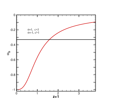
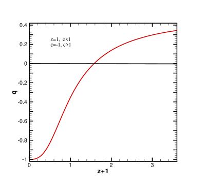
Figure 6: The evolution of $w_{D}$ and the deceleration parameter $q$ versus redshift parameter $z$ for the two branches of DGP braneworld. For both cases $(\epsilon=1,c<1)$ and $(\epsilon=-1,c>1)$, the diagrams are quite similar to each other.

while taking the time derivative of $\rho_{D}=3c^{2}M_{p}^{2}H^{2}$, we find

$$\dot{\rho}_{D}=2\rho_{D}\frac{\dot{H}}{H},$$ (42)

and hence the EoS parameter reads to

$$\omega_{D}=-\frac{2}{3}\frac{\dot{H}}{H^{2}}-1=\frac{-\epsilon\sqrt{\Omega_{r_{c}}}}{1-c^{2}-\epsilon\sqrt{\Omega_{r_{c}}}},$$ (43)

where in the last step, we have used (38) and (39). For $r_{c}\gg 1$ ($\Omega_{r_{c}}\rightarrow 0$), the effects of the extra dimension vanishes and hence we reach to the standard cosmology regime. In this case $\omega_{D}\rightarrow 0$, which is an expected result. This is due to the fact that in the absence of the interaction, the choice of $L=H^{-1}$ leads to a wrong EoS, namely that of dust Li , and hence this choice for the IR cutoff in standard cosmology cannot leads to the accelerated expansion. However, from (43) we see that in the DGP braneworld, the natural choice for the IR cutoff in flat Universe, namely the Hubble radius $L=H^{-1}$, can produce the accelerated expansion. This is one of the interesting results we find in this paper.

The deceleration parameter is also obtained as

$$q=-1-\frac{\dot{H}}{H^{2}}=\frac{1}{2}-\frac{3\epsilon\sqrt{\Omega_{r_{c}}}}{2(1-c^{2}-\epsilon\sqrt{\Omega_{r_{c}}})}.$$ (44)

The evolution of $\omega_{D}$ and $q$ are plotted numerically in figure 6, where we consider two branches of DGP braneworld $\epsilon=1$ and $\epsilon=-1$ with different values of $c$. In order to have reasonable behaviour for the evolution of the DE during the history of the Universe, we should take $c<1$ in case of $\epsilon=1$, while $c>1$ in case of $\epsilon=-1$. For both cases diagrams have similar behavior. From figure 6, we find that for $\epsilon=\pm 1$ we have a transition from deceleration to acceleration phase around $z\approx 0.6$. From figure 6 one can see that EoS parameter $\omega_{D}$ gradually tend to $-1$ with the evolution of the Universe, while it is larger than $-1$ throughout the evolution of Universe, which is an indication for quintessence behavior Cai2 .

Taking the time derivative of Eq. (39) and using Eqs. (34) and (35), we arrive at

$$\frac{\ddot{H}}{H^{3}}=-\Big{(}\frac{\dot{H}}{H^{2}}\Big{)}^{2}\frac{\epsilon\sqrt{\Omega_{r_{c}}}}{(1-c^{2}-\epsilon\sqrt{\Omega_{r_{c}}})}+\frac{9(1-c^{2}-2\epsilon\sqrt{\Omega_{r_{c}}})}{2(1-c^{2}-\epsilon\sqrt{\Omega_{r_{c}}})}.$$ (45)

Using Eqs. (39), (44) and (45), after some calculations, we obtain the statefinder pair parameters as

$$r = 1+3\frac{\dot{H}}{H^{2}}+\frac{\ddot{H}}{H^{3}}=1-\frac{9\epsilon\sqrt{\Omega_{r_{c}}}(1-c^{2}-2\epsilon\sqrt{\Omega_{r_{c}}})^{2}}{4(1-c^{2}-\epsilon\sqrt{\Omega_{r_{c}}})^{3}},$$ (46)

$$s = \frac{r-1}{3(q-1/2)}=\frac{(1-c^{2}-2\epsilon\sqrt{\Omega_{r_{c}}})^{2}}{2(1-c^{2}-\epsilon\sqrt{\Omega_{r_{c}}})^{2}}.$$ (47)

Next, we choose the GO cutoff for the HDE density in the framework of the DGP braneworld. We restrict our study to the current cosmological epoch, and hence we are not considering the contributions from matter and radiation by assuming that the DE dominates, thus the Friedman equation becomes simpler. Substituting (17) into Friedmann equation (32), we can obtain the differential equation for the Hubble parameter as

$$H^{2}(1-\alpha)-\frac{\epsilon}{r_{c}}H-\beta\dot{H}=0.$$ (48)

Solving this equation, the Hubble parameter is obtained as

$$H(t)=\frac{\epsilon}{r_{\rm c}(1-\alpha)+c_{1}\epsilon e^{\frac{\epsilon t}{\beta r_{\rm c}}}},$$ (49)

where $c_{1}$ is a constant of integration. Since for $r_{\rm c}\gg 1$, the effects of the extra dimension should be disappeared and the result of Granda , namely

$$H(t)=\frac{\beta}{\alpha-1}\frac{1}{t},$$ (50)

must be restored, thus the constant $c_{1}$ should be chosen as Gaffari

$$c_{1}=\frac{r_{\rm c}(\alpha-1)}{\epsilon}.$$ (51)

Substituting $c_{1}$ in Eq. (49), we obtain

$$H(t)=\frac{\epsilon}{r_{\rm c}(1-\alpha)(1-e^{\frac{\epsilon t}{\beta r_{c}}})}.$$ (52)

In term of the redshift parameter, we have Gaffari

$$H(z) = \frac{\epsilon}{r_{\rm c}(1-\alpha)}\left[1+(1+z)^{\frac{\alpha-1}{\beta}}\right].$$ (53)

Solving (52) for the scale factor, yields

$$a(t)=a_{0}\Big{(}e^{\frac{-\epsilon t}{\beta r_{c}}}-1\Big{)}^{\frac{\beta}{\alpha-1}}.$$ (54)

Taking the time derivative of Eq. (52), we arrive at

$$\dot{H} = \frac{e^{\frac{\epsilon t}{\beta r_{c}}}}{\beta r_{c}^{2}(1-\alpha)(1-e^{\frac{\epsilon t}{\beta r_{c}}})^{2}},$$ (55)

$$\ddot{H} = \frac{\epsilon e^{\frac{\epsilon t}{\beta r_{c}}}}{\beta^{2}r_{c}^{3}(1-\alpha)(1-e^{\frac{\epsilon t}{\beta r_{c}}})^{2}}\Big{(}1+\frac{2e^{\frac{\epsilon t}{\beta r_{c}}}}{1-e^{\frac{\epsilon t}{\beta r_{c}}}}\Big{)}.$$ (56)

Therefore, it is easy to show that

$$\frac{\dot{H}}{H^{2}} = \frac{1-\alpha}{\beta}e^{\frac{\epsilon t}{\beta r_{c}}}$$ (57)

$$\frac{\ddot{H}}{H^{3}} = \frac{(1-\alpha)^{2}}{\beta^{2}}e^{\frac{\epsilon t}{\beta r_{c}}}\Big{(}1+e^{\frac{\epsilon t}{\beta r_{c}}}\Big{)}$$ (58)

In this case the EoS and the deceleration parameters are obtained as Gaffari

$$\omega_{D}(z)=-1-\frac{1-\alpha}{3\beta}\Big{[}\frac{(1+\alpha)(1+z)^{\frac{1-\alpha}{\beta}}+2}{(1+(1+z)^{\frac{1-\alpha}{\beta}})(1+\alpha(1+z)^{\frac{1-\alpha}{\beta}})}\Big{]},$$ (59)

$$q(z)=-1-\frac{1-\alpha}{\beta\left[1+(1+z)^{\frac{1-\alpha}{\beta}}\right]}.$$ (60)

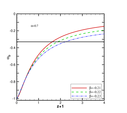
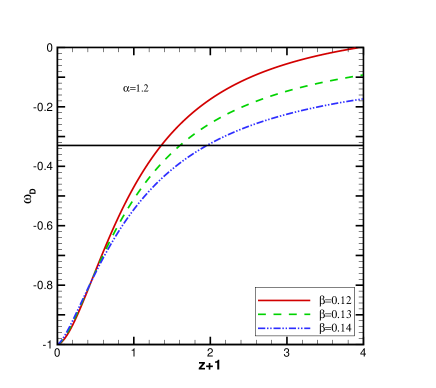
Figure 7: The evolution of $w_{D}$ versus redshift parameter $z$ for HDE with GO cutoff in DGP braneworld. Left panel corresponds to $\alpha<1$ and $\beta<0$, while the right panel shows the case $\alpha>1$ and $\beta>0$.

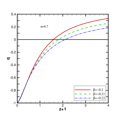
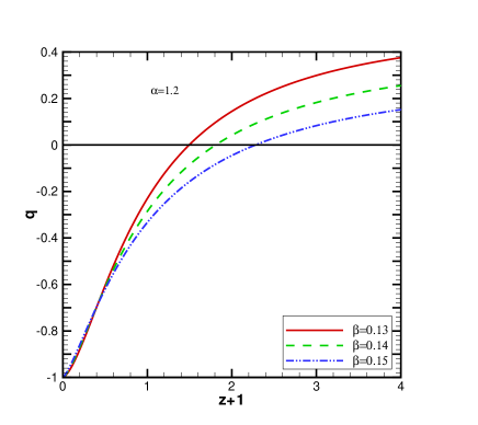
Figure 8: The evolution of the deceleration parameter $q$ versus redshift parameter $z$ for HDE with GO cutoff in DGP braneworld. Left panel corresponds to $\alpha<1$ and $\beta<0$, while the right panel shows the case $\alpha>1$ and $\beta>0$.

To check the limit of (59) in standard cosmology where $r_{c}\gg 1$, we note from Eq. (54) and relation $a/a_{0}=(1+z)^{-1}$ that $(a/a_{0})^{\frac{\alpha-1}{\beta}}=(1+z)^{\frac{1-\alpha}{\beta}}\rightarrow 0$, as $r_{c}\gg 1$. Therefore, (59) reduces to

$$\omega_{D}=-1+\frac{2}{3}\frac{\alpha-1}{\beta},$$ (61)

which is exactly the result obtained in Granda . It is important to note that the EoS parameter of HDE with GO cutoff in DGP braneworld scenario varies with time. Thus, it seems that the presence of the extra dimension brings rich physics. For $\alpha=1$ we have $\omega_{D}=-1$, similar to the cosmological constant. The case with $\alpha<1$ and $\alpha>1$ should be considered separately. In the first case where $\alpha<1$, we find that the EoS parameter can explain the acceleration of the Universe provided $\beta<0$. In the second case where $\alpha>1$, the accelerated expansion can be achieved for $\beta>0$. In both cases, our Universe has a transition from deceleration to the acceleration phase around $0.4\leq z\leq 1$, compatible with the recent observations Daly ; Kom1 ; Kom2 , and mimics the cosmological constant at the late time. In figures (7) and (8) we have shown the evolution of the EoS and the deceleration parameter for HDE with GO cutoff in DGP braneworld.

Combining Eqs. (57) and (58) with (3) and (14), after using Eqs. (54) and (60), we obtain the statefinder pair parameters as

$$r = 1+(1-\alpha)\Big{[}\frac{3\beta(a^{\frac{\alpha-1}{\beta}}+1)+(1-\alpha)(2+a^{\frac{\alpha-1}{\beta}})}{\beta^{2}(a^{\frac{\alpha-1}{\beta}}+1)^{2}}\Big{]},$$ (62)

$$s = \frac{\alpha-1}{6\beta}-\frac{(\alpha-1)^{2}}{3\beta}\frac{2({1+a^{\frac{\alpha-1}{\beta}}})+1}{\Big{(}3\beta(1+a^{\frac{\alpha-1}{\beta}})+2(1-\alpha)\Big{)}(1+a^{\frac{\alpha-1}{\beta}})}.$$ (63)

For $\alpha=1$ we have $\{r,s\}=\{1,0\}$. In term of the redshift parameter, $1+z=a^{-1}$, with $a_{0}=1$ for present time, Eqs. (62) and (63) takes the form

$$r = 1+(1-\alpha)\Big{[}\frac{3\beta((1+z)^{\frac{1-\alpha}{\beta}}+1)+(1-\alpha)(2+(1+z)^{\frac{1-\alpha}{\beta}})}{\beta^{2}((1+z)^{\frac{1-\alpha}{\beta}}+1)^{2}}\Big{]},$$ (64)

$$s = \frac{\alpha-1}{6\beta}-\frac{(\alpha-1)^{2}}{3\beta}\frac{2({1+(1+z)^{\frac{1-\alpha}{\beta}}})+1}{\Big{(}3\beta(1+(1+z)^{\frac{1-\alpha}{\beta}})+2(1-\alpha)\Big{)}(1+(1+z)^{\frac{1-\alpha}{\beta}})}.$$ (65)

The evolution of the statefinder pair parameters for HDE with GO cutoff in the framework of DGP braneworld have been shown in figures 9-12. Interestingly enough, from figure (11) we see that $r$ diverge as $q\rightarrow 1/2$, which corresponds to the matter dominated Universe, and mimics the cosmological constant, namely $r=1,q=-1$, in the far future where $z\rightarrow 0$.

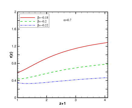
Figure 9: The evolution of the statefinder parameter $r$ versus $1+z$ for HDE with GO cutoff in DGP braneworld.

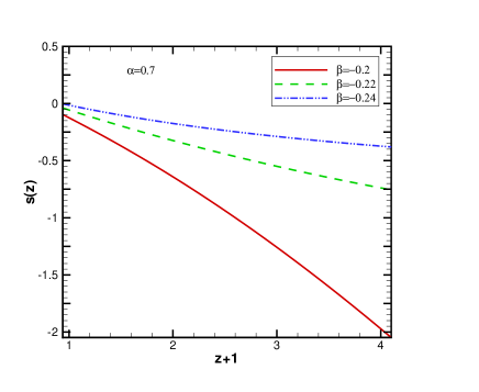
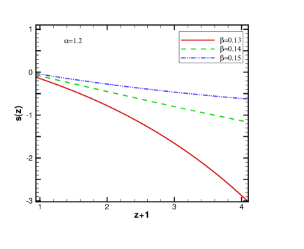
Figure 10: The evolution of the statefinder parameter $s$ versus $1+z$ for HDE with GO cutoff in DGP braneworld.

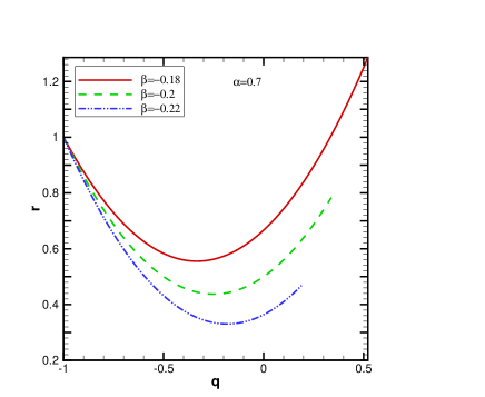
Figure 11: The evolution of the statefinder parameter $r$ versus deceleration parameter $q$ for HDE with GO cutoff in DGP braneworld.

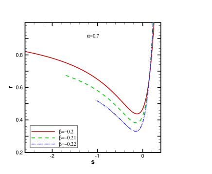
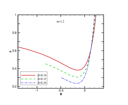
Figure 12: The evolution of the statefinder parameter $r$ versus $s$ for for HDE with GO cutoff in DGP braneworld.

IV Conclusions and discussion

Following the discovery of the accelerated expansion of the Universe, many DE models have been introduced to explain such a cosmic acceleration. In order to discriminate various DE models, the statefinder diagnosis pair parameters $\{r,s\}$ was introduced Sahni ; Alam . This diagnostic is constructed from scale factor $a(t)$ and its derivatives up to the third order. It was argued that trajectories in the $r-s$ plane correspond to a wide variety of DE models. The spatially flat $\Lambda$CDM scenario corresponds to a fixed point $\{r,s\}=\{1,0\}$ in the statefinder diagnosis diagram. Departure of a given DE model from this fixed point provides a good way for establishing the statefinder of the presented model from $\Lambda$CDM.

In this paper, we have considered HDE in standard cosmology as well as DGP braneworld. We have chosen the Hubble radius $L=H^{-1}$ and the GO cutoff $L=(\alpha\dot{H}+\beta H^{2})^{-1/2}$, inspired by Ricci scalar curvature of flat FRW universe, as the system’s IR cutoff . We have investigated the evolution of the EoS, deceleration and statefinder parameters. We found that in standard cosmology for both proposed cutoff, the statefinder pair parameters $\{r,s\}$ become constant depending on the model parameters and with suitably choosing the parameters they restore those of $\Lambda$CDM model. However, in the framework of DGP braneworld, the situation become completely different and some interesting results can be observed. Interestingly enough, we found that although choosing $L=H^{-1}$ as the IR cutoff, in the absence of interaction, leads to the wrong EoS of dust $w_{D}=0$ Li , here because of the effects of extra dimensions the natural choice for IR cutoff in flat Universe, namely the Hubble radius $L=H^{-1}$, can lead to an accelerated expanding Universe. In this case $w_{D}$ and $q$, as well as the pair parameters $\{r,s\}$ depend on $\Omega_{r_{c}}={1}/({4H^{2}r_{c}^{2}})$. For GO cutoff in DGP braneworld, the cosmological parameters can be obtained as the function of redshift parameter $z$, and in case of $\alpha=0$, we reach to $\{r,s\}=\{1,0\}$, as expected. We have plotted the behaviour of $\{r,s\}$ and observed that $r$ diverges at the past as $q\rightarrow 1/2$, which corresponds to the matter dominated era, and mimics the cosmological constant with $r=1,q=-1$ in the future.