Analytical theory for proton correlations in common water ice $I_{h}$

Abstract

We provide a fully analytical microscopic theory for the proton correlations in water ice $I_{h}$. We compute the full diffuse elastic neutron scattering structure factor, which we find to be in excellent quantitative agreement with Monte Carlo simulations. It is also in remarkable qualitative agreement with experiment, in the absence of any fitting parameters. Our theory thus provides a tractable analytical starting point to account for more delicate features of the proton correlations in water ice. In addition, it directly determines an effective field theory of water ice as a topological phase.

The different phases of matter are commonly illustrated through the example of ice, water and steam. However, common water ice has for a long time been known to be a most untypical solid,petrwhit exhibiting Pauling’s celebrated ’zero-point entropy’paulingentropy as the protons in fact remaining intricately partially disordered, with only the oxygens being associated with a regular arrangement on a lattice.

Nowadays, we can address detailed questions about the microscopic nature of water ice. In its most common form, ice $I_{h}$, the fourfold coordinated oxygen atoms form a hydrogen-bonded wurtzite structure.petrwhit One of the Bernal-Fowler ice rules state that each oxygen atom has two protons sitting close to it, and the other two are further away (Fig. 1). Being subject to these ice rules, proton locations are thus not entirely random, and the nature of correlations between them has been a topic of study for a long time, in theory, simulation and experimentpetrwhit ; fradice ; expice ; mcice ; qu_ice ; ice_gren . In this context, the fact that an ice rule can be cast as a conservation law was identified as leading to a characteristic pinch-point feature in the structure factor of ice.villainice ; YoungAxe ; henleycoulomb

However, beyond this long-wavelength insight, little analytical progress has occurred, thus providing only limited analytical backup for the existing extensive numerical modelling, which does exhibit satisfactory agreement with experiment.

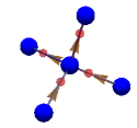
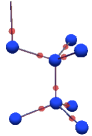
Figure 1: Protons in an ice crystal. The locations of the oxygen ions approximate a bipartite wurtzite structure (with identical atoms on the two sublattices, also known as ’hexagonal diamond’).vesta Like in the case of cubic ice, where they form a (cubic) diamond lattice, they are four-fold coordinated with the midpoints of the bonds forming tetrahedra. However, the tetrahedra are arranged differently: the relation between these two lattice types is the same as between hexagonal and cubic close packed crystal systems The oxygens are bonded by the red hydrogen/deuterium ions. The latter are not ordered but are subject to the ice rule that each oxygen has two sitting closeby and two further away, so that the $\{$D/H$\}$₂O molecules ‘retain their identity’ even in the solid. This implies an emergent conservation law for the flux denoted by the brown arrows on the midpoints of the bonds, defined to point towards the proton on the bond (middle): each oxygen ion sees the same amount of flux arriving as leaving. Right: sketch of a unit cell with an example of an allowed configuration of the eight protons it contains.

In recent years, much progress in this direction has occurred in the context of the family of magnetic compounds known as the spin iceshuse ; hermele ; pyrdip ; henley ; qu_ice , for reviews see Refs. henleycoulomb, ; cmsARCM, These have benefitted much from transfer from water ice – including receiving their name. In this work, we aim to reverse the direction of this transfer. This partially builds on insights gained in considering spin ice as a model system for topological phases in condensed matter physics – with water ice probably is the most ubiquitous material exhibiting topologically nontrivial behaviour.

In the following, we first present our analytical theory of the proton correlations in water ice, which we contrast to simulations and experiment. We then briefly put this in the context of topological phenomena in condensed matter physics, in particular by deriving an accurate value of the coupling constant of the long-wavelength action for water ice $I_{h}$.

Structure factor: We consider the diffuse scattering away from the Bragg peaks, as the peaks are encode the ‘average’ underlying arrangement of the ions rather than the displacement of the protons from it, which is what we are interested in. Whereas X-ray scattering is sensitive to the charge of the ions and their electrons, and thus is not ideally suited for detecting protons, neutrons are a suitable probe, especially for deuterated ice, D₂O.

Our theory neglects thermal fluctuations and any static disorder that may be present in a given sample and focuses on implementing the abovementioned ice rules The basic degree of freedom is thus the location $\mathbf{r}_{i\alpha}$ of the proton on bond $\alpha$ of unit cell $i$. We allow two possible proton positions for each bond – closer to either one or the other oxygen being bonded. This is parametrised by an Ising variable $S=\pm 1$:

$$\mathbf{r}_{i\alpha}=\mathbf{r}^{0}_{i\alpha}+S_{i\alpha}a\hat{\mathbf{e}}_{\alpha},$$

where $\mathbf{r}^{0}_{i\alpha}$ are the midpoints of the oxygen-oxygen bonds forming a network of corner-sharing tetrahedra, $S_{i\alpha}$ are the Ising “spins” living at the midpoints of the oxygen-oxygen bonds, $a$ is the absolute value of the proton displacement relative to the midpoint, and $\hat{\mathbf{e}}_{\alpha}$ are unit vectors along the oxygen-oxygen bonds. The index $\alpha$ runs from 1 to 8 as the unit cell of the wurtzite structure contains 8 sites.

The ice rules are enforced by devising a Hamiltonian which penalises configurations that do not obey them, and studying the resulting ground state correlations. How to obtain this has been established in the context of spin ice pyrdip . The precise form of the Hamiltonian, with details of the analysis sketched below, is relegated to the appendix.

The quantity we compute is the structure factor, which is proportional to the neutron scattering cross section:

$${\cal S}(\mathbf{q})=\langle|\sum_{i\alpha}b_{i\alpha}e^{i\mathbf{q}\mathbf{r}_{i\alpha}}|^{2}\rangle,$$

where $\mathbf{q}$ is the wave vector change of the neutron, $b_{i\alpha}\equiv b=\text{const}$ is the scattering length, and the brackets denote averaging over all proton configurations obeying the ice rules.

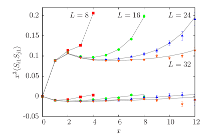
Figure 2: Theory versus Monte Carlo simulations. Correlation function $\langle S_{i1}S_{j1}\rangle$ from Monte Carlo simulations (symbols) compared to our analytical theory (lines) at zero temperature for two inequivalent directions, $[100]$ and $[001]$, and different system sizes $L$. The correlation functions are multiplied by the cube of the distance $x$ for better visibility.

To express the structure factor in terms of the Ising spin correlation function $\langle S_{i\alpha}S_{j\beta}\rangle$, we note

$${\cal S}(\mathbf{q})=b^{2}\sum_{i\alpha,j\beta}\langle e^{ia\mathbf{q}(S_{i\alpha}\hat{\mathbf{e}}_{\alpha}-S_{j\beta}\hat{\mathbf{e}}_{\beta})}\rangle e^{i\mathbf{q}(\mathbf{r}^{0}_{i\alpha}-\mathbf{r}^{0}_{j\beta})}.$$

The spin correlator is absent in one of the following terms

$$\langle e^{ia\mathbf{q}(S_{i\alpha}\hat{\mathbf{e}}_{\alpha}-S_{j\beta}\hat{\mathbf{e}}_{\beta})}\rangle = 2\langle S_{i\alpha}S_{j\beta}\rangle\sin(a\mathbf{q}\hat{\mathbf{e}}_{\alpha})\sin(a\mathbf{q}\hat{\mathbf{e}}_{\beta})$$

$$+ 2\cos(a\mathbf{q}\hat{\mathbf{e}}_{\alpha})\cos(a\mathbf{q}\hat{\mathbf{e}}_{\beta})$$

whence we finally get the diffuse scattering as

$${\cal S}(\mathbf{q})\propto\sum_{i\alpha,j\beta}\langle S_{i\alpha}S_{j\beta}\rangle\sin(a\mathbf{q}\hat{\mathbf{e}}_{\alpha})\sin(a\mathbf{q}\hat{\mathbf{e}}_{\beta})e^{i\mathbf{q}(\mathbf{r}^{0}_{i\alpha}-\mathbf{r}^{0}_{j\beta})}.$$

with the computation of the correlation function $\langle S_{i\alpha}S_{j\beta}\rangle$ carried out in the large-$N$ framework (described in the appendix). This is based on treating relaxing the fixed spin length constraint to one which is only obeyed ‘on average’, but which has the advantage of being exactly soluble. For models closely related to the present ones, this has been shown to be an accurate approximation.pyrdip

Indeed, to demonstrate the accuracy of our evalution of the correlation function $\langle S_{i\alpha}S_{j\beta}\rangle$, we compare Monte Carlo simulations to the analytical expression in Fig. 2. We use the notation for a unit cell containing four oxygen atoms and eight protons. One finds excellent quantitative agreement in different directions, for different distances, even capturing finite-size effects faithfully. The data for finite-size systems with $N_{t}$ spins can be obtained by explicitly solving for an $N_{t}\times N_{t}$-dimensional interaction matrix in real space, or equivalently carrying out a discrete sum over points in reciprocal space.

Comparison to experiment: The analytically obtained neutron scattering structure factor is compared to neutron resultsexpice in different planes in reciprocal space in Figs. 3. The proton displacement was taken to be $a\approx 0.1436R_{\text{OO}}$petrwhit , where $R_{\text{OO}}$ is the distance between the oxygen atoms.

Analytical results compare reasonably well to the experiment, especially in the first few Brillouin zones. In particular, location and orientation of the pinchpoints are given correctly, alongside the general structure of regions with high and low neutron scattering intensity.

One important feature of our theory is thus that there exists an analytical expression for the correlations which can be used as a starting point to understand deviations away from the ideal ice model. By providing an explicit analytical form, this obviates a complex first modelling step (e.g. via numerical fitting procedures to Monte Carlo simulations) and therefore allows for a focus on the physics beyond the ice rules.

Such deviations can take many forms. One is a simple improvement of our modelling of the scattering form factor of the proton/deuterium ion, which we have treated as a pointlike scatterer so far, but whose finite extent and finite-temperature thermal motion will inevitably lead to a change in the structure factor in higher Brillouin zones irregardless of any cooperative physics. Similarly, we have completely omitted the Bragg peaks due to the oxygen ions, which feature prominently in the experimental plots.

More interesting are defects in the lattice structure or in the bonding – violations of the ice rule – which may be static or dynamical. Defects in ice have attracted considerable attention, and much is known about them. In our treatment, there is one natural parameter which can be added to account for the presence of gauge-charged defects (see below), namely an effective correlation length beyond which their presence removes the correlations responsible for the pinch-points, with the resulting width of the pinchpoints reflecting the inverse of this length.

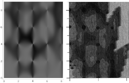
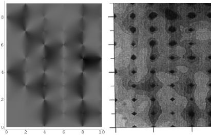
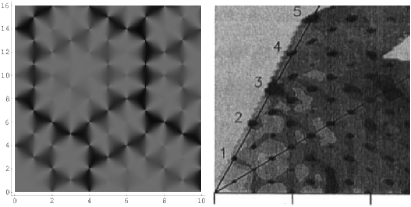
Figure 3: Diffuse neutron scattering in water ice. Shown is the structure factor in the $[h0l]$ (top), $[0kl]$ (middle) and $[hk0]$ (bottom) planes, with dark (light) regions indicating high (low) scattering intensity.fn-convention Left: theoretical results for zero temperature (bottom: Eq. 2). Right: experimental result from D₂O ice expice at 20 K (bottom: 10K). Note the pinchpoint features at the centres of higher Brillouin zones, where areas of high and low scattering intensity meet; these are partially obscured by Bragg peaks in the experimental data.

Long-wavelength theory: The great advantage of our method lies in the fact that it works for all distances as well as a wide variety of lattices. The peculiar nature of the proton correlations become particularly evident from the analytics upon closer inspection, with the pinch-point features in the structure factor visible even in the absence of an explicit identification of an emergent gauge field. However, historically, it was noticed already early onvillainice ; YoungAxe that the pinchpoints in the neutron scattering were due to this conservation law. Basically, the reason this happens is because a field obeying only the constraint $\nabla\cdot{\cal B}=0$, but which is otherwise free, has no longitudinal degrees of freedom, and a pinchpoint is precisely the result of projecting out the longitudinal component of the (otherwise random) proton displacements, in a way which is entirely analogous to how the pinchpoints arise in spin ice huse ; henley . [The field ${\cal B}$ is obtained straightforwardly by drawing an arrow from the midpoint of the bond towards the centre of charge of the proton. Upon identifying these arrows with a unit of an imaginary (lattice) flux, ${\cal B}$,the (lattice) divergence of this flux vanishes, $\nabla\cdot{\cal B}=0$ – the flux is conserved (Fig. 1).]

Via an analogy to magnetostatics, one obtains an effective partition function, where the permeability $\mu_{0}$ of the electromagnetic vacuum is replaced by an emergent permeability (’stiffness’), $K$:

$${\cal S}=\frac{K}{2}\int d^{3}r{\cal B}^{2}\ .$$

This is called topological because the above functional goes along with the deconfined ‘Coulomb’ phase of a classical U(1) gauge theory, which is distinct from a simple disordered phase, while not exhibiting any conventional (crystalline) order for the protons.cmsARCM

As the wurtzite lattice is not cubic (unlike the case of spin ice, which corresponds to ice $I_{c}$), it is not a priori obvious that a single stiffness constant is enough to describe the action of the gauge field, but it turns out that just one stiffness constant is enough, at least approximately. Indeed, the actual value of this stiffness is a priori a free parameter, as it cannot be derived by symmetry considerations alone, instead depending on non-universal details of the model exhibiting an emergent gauge field. Our lattice-based microscopic theory does incorporate such information, so that it can be used to extract an approximate but accurate estimate from its long-wavelength expansion near the pinchpoints. For instance, one can expand Eq. 2 in the Appendix near $q_{x}=q_{y}=0$ and read off, by direct comparison to the predictions from the gauge theory, which have the same functional form:

$$KR_{\text{OO}}^{3}\approx\sqrt{3}/8\ .$$ (1)

This piece of information, together with the general long-wavelength form of the theory, is enough to yield the full asymptotics of the correlation function in real space, which takes the dipolar form,

$$\langle S_{i\alpha}S_{j\beta}\rangle=\frac{1}{4\pi K}\left(\frac{\hat{\mathbf{e}}_{\alpha}\hat{\mathbf{e}}_{\beta}}{r_{ij}^{3}}-\frac{3(\hat{\mathbf{e}}_{\alpha}\mathbf{r}_{ij})(\hat{\mathbf{e}}_{\beta}\mathbf{r}_{ij})}{r_{ij}^{5}}\right).$$

Note that these results imply that the long-range part of the interaction between the protons – which is due to the interactions between the dipole moments of the bonds arising from the asymmetric location of the protons – has an additional component to it which is not of an electrostatic origin, but rather due to the contribution Eq. 1. This would be present even if the protons were electrically neutral, so that neutral particles obeying the ice rules would exhibit the same form of the correlations!

This dichotomy is due to the protons being doubly charged–they have an (intrinsic) electric on top of an (emergent) gauge charge. The latter associated with the emergent conservation law for ${\cal B}$. The former is not the naive ‘electronic’ charge $|e|$, but rather related to the divergence of the electric dipole moment at the location of a defect.NagleUnit ; MoeSonIrrat Charged defects in ice are therefore special in that they are quasiparticles which not only have an irrational electric charge, but also an emergent entropic Coulomb charge.

Final remarks: It is remarkable that a material as well-known as water ice should be an embodiment of the topological physics of unconventional types of order that has come into focus relatively recently. For future work, it would be most desirable to obtain new neutron scattering data on a par with the recent X-ray work,ice_gren in order to allow for a more detailed and quantitative understanding of the microscopic proton distribution in water ice, beyond the analysis presented there; here we have provided a parameter-free analytical theory encoding the Bernal-Fowler ice rules, which is applicable at all lengthscales and can be used as a solid basis for including more delicate effects in a simple framework. It is a tantalising prospect that such analytical theories might be more generally useful for modelling diffuse neutron scattering experiments.

Acknowledgements: This work was in part supported by the Helmholtz Virtual Institute VI-521 ”New states of matter and their excitations” (R.M.). This work was supported by NSF Grant No. DMR-1311781, the Alexander von Humboldt Foundation and the German Science Foundation (DFG) via the Gottfried Wilhelm Leibniz Prize Programme at MPI-PKS (S.L.S.). ORNL is managed by UT-Battelle, LLC, under contract DE-AC05-00OR22725 for the U.S. Department of Energy (D.A.T.).

Note added: At the same time as this work, a preprint by Benton et al. appearedBentonIce on the proton correlations in water ice, in particular in the presence of quantum dynamics.

Appendix A Large-$N$ theory for water ice $I_{h}$

The (approximate) oxygen positions in water ice can be used to define a regular wurtzite structure with a unit cell containing four oxygen ions, to which contains 8 protons (spins) are associated. The effective interaction matrix enforcing the ice rule therefore has dimension $8\times 8$ and takes the form

$${\cal H}=\frac{1}{T}\left(\begin{matrix}2&2b&2c&f&f^{*}&0&0&0\cr 2b&2&2\bar{c}&g&g^{*}&0&0&0\cr 2c&2\bar{c}&2&h&h^{*}&0&0&0\cr f^{*}&g^{*}&h^{*}&2&0&\bar{f}&\bar{g}&\bar{h}\cr f&g&h&0&2&\bar{f}^{*}&\bar{g}^{*}&\bar{h}^{*}\cr 0&0&0&\bar{f}^{*}&\bar{f}&2&2b&2c\cr 0&0&0&\bar{g}^{*}&\bar{g}&2b&2&2\bar{c}\cr 0&0&0&\bar{h}^{*}&\bar{h}&2c&2\bar{c}&2\cr\end{matrix}\right),$$

where $b=\cos(q_{x}/2\sqrt{2})$, $c=\cos(q_{x}/4\sqrt{2}+\sqrt{3}q_{y}/4\sqrt{2})$, $\bar{c}=\cos(q_{x}/4\sqrt{2}-\sqrt{3}q_{y}/4\sqrt{2})$, $f=\exp[i(q_{x}/4\sqrt{2}+q_{y}/4\sqrt{6}+q_{z}/2\sqrt{3})]$, $g=\exp[i(-q_{x}/4\sqrt{2}+q_{y}/4\sqrt{6}+q_{z}/2\sqrt{3})]$, $h=\exp[i(-q_{y}/2\sqrt{6}+q_{z}/2\sqrt{3})]$, $\bar{f}=\exp[i(-q_{x}/4\sqrt{2}-q_{y}/4\sqrt{6}+q_{z}/2\sqrt{3})]$, $\bar{g}=\exp[i(q_{x}/4\sqrt{2}-q_{y}/4\sqrt{6}+q_{z}/2\sqrt{3})]$, $\bar{h}=\exp[i(q_{y}/2\sqrt{6}+q_{z}/2\sqrt{3})]$, $*$ denotes complex conjugation, and $T$ is the temperature.

The Fourier transform of the Ising spin correlation function $G_{\alpha\beta}(x)=\langle S_{i\alpha}S_{j\beta}\rangle$ can be written in the large-$N$ theory approximation asgarcan ; pyrdip

$$G_{\alpha\beta}(\mathbf{q})=\sum_{\mu=1}^{8}\frac{U_{\mathbf{q},\alpha\mu}U_{\mathbf{q},\beta\mu}^{\dagger}}{\lambda+e_{\mathbf{q},\mu}},$$

where $e_{\mathbf{q},\rho}$ are the eigenvalues of the interaction matrix ${\cal H}$, $U_{\mathbf{q},\alpha\mu}$ is a unitary transformation that diagonalizes the interaction matrix, and $\lambda$ is determined by the equation

$$8n=\sum_{\mathbf{q},\mu}\frac{1}{\lambda+e_{\mathbf{q},\mu}},$$

where $n$ is the number of unit cells. In the limit of low temperature, only the four flat bands of the interaction matrix contribute to the correlation function and $\lambda\rightarrow 1/2$.

The structure factor can then be straightforwardly obtained analytically, although it turns out that its form is rather lengthy. In some high-symmetry planes, it however, becomes quite simple. For instance, in the $[hk0]$ plane (with ${\cal C}_{x}=\cos\left(\frac{aq_{x}}{2\sqrt{2}}\right)$ and ${\cal C}_{y}=\cos\left(\frac{aq_{y}}{2\sqrt{6}}\right)$ and ${\cal C}\leftrightarrow{\cal S}$ for $\cos\leftrightarrow\sin$):

$$\frac{\left[2{\cal C}_{x}{\cal S}_{y}\cos\left(\frac{1}{4}\sqrt{\frac{3}{2}}q_{y}\right)\sin\left(\frac{q_{x}}{4\sqrt{2}}\right)-2{\cal C}_{y}{\cal S}_{x}\cos\left(\frac{q_{x}}{4\sqrt{2}}\right)\sin\left(\frac{1}{4}\sqrt{\frac{3}{2}}q_{y}\right)+2{\cal C}_{y}{\cal S}_{y}\sin\left(\frac{q_{x}}{2\sqrt{2}}\right)\right]^{2}}{3-\cos\left(\frac{q_{x}}{\sqrt{2}}\right)-2\cos\left(\frac{q_{x}}{2\sqrt{2}}\right)\cos\left(\frac{1}{2}\sqrt{\frac{3}{2}}q_{y}\right)}.$$ (2)

References

- (1) V. F. Petrenko and R. W. Whitworth, Physics of ice (Oxford University Press, Oxford, 1999).
- (2) L. Pauling, J. Am. Chem. Soc. 57 (12), 2680 2684 (1935).
- (3) A. H. Castro Neto, P. Pujol and Eduardo Fradkin, Phys. Rev. B 74, 024302 (2006).
- (4) J. C. Li, V. M. Nield, D. K. Ross, R. W. Whitworth, C. C. Wilson and D. A. Keen, Phil. Mag. B 69, 1173 (1994).
- (5) Nic Shannon, Olga Sikora, Frank Pollmann, Karlo Penc and Peter Fulde, Phys. Rev. Lett. 108, 067204 (2012).
- (6) B. Wehinger, D. Chernyshov, M. Krisch, S. Bulat, V. Ezhov, and A. Bosak, J Phys.: Condens. Matter 26, 265401 (2014).
- (7) M. N. Beverley and V. M. Nield, J. Phys.: Condens. Matter 9, 5145 (1997) .
- (8) J. Villain, Solid State Communications 10 (10), 967 (1972).
- (9) R. Youngblood, J. D. Axe and B. M. McCoy, Phys. Rev. B21, 5212 (1980).
- (10) C. L. Henley, Ann. Rev. Cond. Matt. Phys., 1 179 (2010).
- (11) D. A. Huse, W. Krauth, R. Moessner and S. L. Sondhi Phys. Rev. Lett. 91, 167004 (2003).
- (12) M. Hermele, M. P. A. Fisher and L. Balents, Phys. Rev. B69, 064404 (2004).
- (13) S. V. Isakov, K. Gregor, R. Moessner and S. L. Sondhi, Phys. Rev. Lett. 93, 167204 (2004).
- (14) C. L. Henley, Phys. Rev. B71, 014424 (2005).
- (15) C. Castelnovo, R. Moessner and S. L. Sondhi, Ann. Rev. Cond. Matt. Phys. 3, 35 (2012).
- (16) K. Momma and F. Izumi, J. Appl. Cryst. 44, 1272 (2011).
- (17) Our work and Ref. expice, use different conventions for indexing the lattice; the figures, however, show the same parts of reciprocal space.
- (18) J. F. Nagle, Chem. Phys. 43, 317 (1979)
- (19) R. Moessner and S.L. Sondhi, Phys. Rev. Lett. 105, 166401 (2010).
- (20) D. A. Garanin and B. Canals, Phys. Rev. B59, 443 (1999).
- (21) O. Benton, O. Sikora and N. Shannon, arXiv:1504.04158.