Energy reconstruction of hadron-initiated showers of ultra-high energy cosmic rays

Abstract

The current methods to determine the primary energy of ultra-high energy cosmic rays (UHECRs) are different when dealing with hadron or photon primaries. The current experiments combine two different techniques, an array of surface detectors and fluorescence telescopes. The latter allow an almost calorimetric measurement of the primary energy. Thus, hadron-initiated showers detected by both type of detectors are used to calibrate the energy estimator from the surface array (usually the interpolated signal at a certain distance from the shower core $S(r_{0})$) with the primary energy. On the other hand, this calibration is not feasible when searching for photon primaries since no high energy photon has been unambiguously detected so far. Therefore, pure Monte Carlo parametrizations are used instead.

In this work, we present a new method to determine the primary energy of hadron-induced showers in a hybrid experiment based on a technique previously developed for photon primaries. It consists on a set of calibration curves that relate the surface energy estimator, $S(r_{0})$, and the depth of maximum development of the shower, $X_{max}$, obtained from the fluorescence telescopes. Then, the primary energy can be determined from pure surface information since $S(r_{0})$ and the zenith angle of the incoming shower are only needed. Considering a mixed sample of ultra-high energy proton and iron primaries and taking into account the reconstruction uncertainties and shower to shower fluctuations, we demonstrate that the primary energy may be determined with a systematic uncertainty below 1$\%$ and resolution around 16$\%$ in the energy range from 10^18.5 to 10^19.6 eV. Several array geometries, the shape of the energy error distributions and the uncertainties due to the unknown composition of the primary flux have been analyzed as well.

1 Introduction

The energy spectrum of cosmic rays extends by more than 10 orders of magnitude from below 1 GeV to more than 10²⁰ eV. The energy spectrum follows a power law as $E^{-\gamma}$, where $\gamma$ is around 3.0 in the whole energy range. It is so steep that direct measurements are not feasible above 100 TeV. At higher energies, the properties of the primary cosmic ray are determined indirectly from the measurement of the extensive air shower (EAS) it produces after colliding with molecules of the atmosphere.

The highest energy EASs have been traditionally studied using two different techniques. The first one is based on telescopes that collect the fluorescence light emitted by atmospheric Nitrogen molecules excited by secondary particles of the EAS (e.g., Fly’s Eye, HiRes). This allows to determine the longitudinal profile of the shower and it is considered to be close to a calorimetric measurement of the UHECR primary energy. However, fluorescence light can only be observed during moonless nights and, consequently, this technique can only be applied to $\sim 13\%$ of the incoming events [1]. The second technique involves an array of detectors located at ground level, mainly scintillators (e.g., Volcano Ranch, AGASA, KASCADE) or water Cherenkov tanks (e.g., Haverah Park), whose duty cycle is close to $100\%$. Thus, the lateral distribution of secondary particles at ground level can be inferred from the discrete sampling of the shower front. The lateral distribution is fitted assuming an appropriate parametrization (called the lateral distribution function, LDF). The interpolated signal at a certain optimum distance, $S(r_{0})$, is used as the energy estimator, which can be related to the primary energy thorough, for instance, Monte Carlo (MC) parametrizations. The optimum distance, $r_{0}$, is traditionally fixed for each detector since it is assumed to be only dependent on the array spacing and geometry [2], although some studies suggest the convenience of calculating the optimum distance for each individual shower taking into account its primary energy and direction [3].

The current experiments, on the other hand, use hybrid techniques for $S(r_{0})$ calibration. The Pierre Auger Observatory [4], taking data since 2004, pioneers the simultaneous use of water Cherenkov detectors and fluorescence telescopes, while the Telescope Array Observatory [5], operating since 2008, combines scintillators and telescopes. Events detected simultaneously by both the surface and fluorescence detectors are called hybrid. Hybrid events allow the calibration of $S(r_{0})$ with primary cosmic ray energy [6]. Thus, the energy of each event detected by the surface detector alone can be determined almost independently of MC simulations. Systematic errors in energy estimate are greatly reduced in this way [7, 8]. These calibrations assume that the primaries are nuclei and, therefore, they cannot be directly applied to photon-initiated showers. In addition, no photon event has been unambiguously identified up to now by any experiment so a proper calibration for photons is not possible with this technique. Therefore, each experiment relies on MC simulations to infer the primary energy of photon events [9, 10, 11, 12, 13].

The method used for photon searches by Auger in Ref. [13] was first proposed in Ref. [14]. This method takes into account the well-known universality of the electromagnetic component of EAS [15, 16, 17] and the small muon fraction of the photon-initiated showers. The calibration curve, that is obtained from MC simulations, relates $S(r_{0})$, the zenith angle of the incoming shower, $\theta$, and $X_{max}$. Thus, the primary energy of photon primaries can be determined with resolution of $\sim$20-25$\%$ [13, 14].

In this work, we show how to modify that method to be applicable to hadron-initiated showers where the muon component is significant, especially, in case of water Cherenkov arrays which enhanced their contribution to the total measured signal. The additional advantage is that the same method could be used to infer the primary energy for both, photon and hadron showers. Moreover, in case of hadron-initiated showers the method can be calibrated with hybrid events reducing the systematic uncertainties coming from the high energy hadronic models used for shower simulations.

2 Shower and detector simulations

The simulation of the atmospheric showers is performed with the AIRES Monte Carlo program (version 2.8.4a) [18] using QGSJET-II-03 [19] as the hadronic interaction model. The input primary energy goes from $\log(E/eV)$ $=$ $18.5$ to $19.6$ in $0.1$ steps. Approximately $2000$ events have been simulated per energy bin for both, proton and iron primaries. The zenith angle has been selected following a sine-cosine distribution from $0$ to $60$ degrees, while the azimuth angle is uniformly distributed from $0$ to $360$ degrees. $X_{max}$ is obtained from these simulations.

Given the energy, the zenith and azimuth angles of the shower, the detector response is simulated with our own code, previously tested in Refs. [3, 20, 21]. Following the original proposal in Ref. [14], we select a triangular array of cherenkov detectors separated 1.5 km and $S(r_{0}=1000\textrm{m})\equiv S(1000)$ as the energy estimator. The real core is randomly located inside an elementary cell while the reconstructed core position is determined by fluctuating the real one with a Gaussian function whose standard deviation depends on the primary energy, composition and the distance between detectors (see Ref. [3] for more details).

The signal collected at each station for a given shower is set assuming a true lateral distribution function of the form,

$$S(r)=S(1000)\times\left(\frac{r}{r_{0}}\right)^{-\beta}\times\left(\frac{r+r_{s}}{r_{0}+r_{s}}\right)^{-\beta},$$ (1)

where $r_{s}$ = 700 m, $r_{0}$=1000 m, the distance to the shower axis $r$ is in meters, $S(1000)$ is in VEM (vertical equivalent muons, unit for the energy deposited by a vertical muon in a water tank [4]) and $\beta(\theta,S(1000))$ is given by (based on work by T. Schmidt et al. [22] as presented in [23]),

$$\beta(\theta,S(1000))=\left\{\begin{array}[]{ll}a+b(\sec\theta-1)&\textrm{if}\sec\theta<1.55\\ a+b(\sec\theta-1)&\\ +f(\sec\theta-1.55)^{2}&\textrm{if}\sec\theta>1.55\end{array}\right.$$ (2)

where $a=2.26+0.195\log(e)$, $b=-0.98$, $c=0.37-0.51\sec\theta+0.30\sec^{2}\theta$, $d=1.27-0.27\sec\theta+0.08\sec^{2}\theta$, $e=c\ S(1000)^{d}$ and $f=-0.29$.

A realistic $S(1000)$ to be used in Eqs. (1) and (2) is obtained from,

$$E = A\ (S_{38})^{B},$$

$$S(1000)(\theta) = S_{38}\times\left[1+Cx-Dx^{2}\right],$$ (3)

where $x=\cos^{2}(\theta)-\cos^{2}(38^{o})$. $A$, $B$, $C$ and $D$ are constants given in Ref. [23] for QGSJetII-03, iron and proton primaries. In addition, shower to shower fluctuations for each primary are emulated by fluctuating the value from Eq. (2) with a Gaussian distribution whose standard deviation is taken from Fig. 3 in Ref. [24].

Finally, the signal assigned to each station is fluctuated using a Poissonian distribution whose mean is given by the true LDF. We adopt $S_{th}=3.0$ VEM and $S_{sat}=1221$ VEM as trigger and saturation thresholds respectively [3].

Next, the lateral distribution of particles is fitted using a functional form given by,

$$\log S(r)=a_{1}+a_{2}\left[\log\left(\frac{r}{r_{0}}\right)+\log\left(\frac{r+r_{s}}{r_{0}+r_{s}}\right)\right],$$ (4)

where the slope of the LDF and the normalization constant are free parameters while the core position is fixed in the reconstructed one. The values of $\chi^{2}$/ndf are good if at least 3 stations are included in the fit, a minimum condition for shower reconstruction that is fulfilled for almost every event above the energy threshold of the detector. Finally, the reconstructed $S(1000)$ is determined as the interpolated value from the fit at $1000$ meters from the shower axis. In this method, event by event fluctuations and reconstruction uncertainties are properly taken into account.

The problem of saturation is common to all surface arrays, specially when dealing with high energy vertical showers. The consequent lack of detectors close to the core produces large uncertainties in the LDF fit and affects the reconstructed $S(r_{0})$. The Auger Collaboration, for example, has developed sophisticated algorithms to estimate the signal of a saturated detector [25]. Nevertheless, the analysis of such uncertainties and how to minimize them is beyond the scope of the present work so saturated events are discarded here.

The simulation set has been divided into two samples. In each sample, an equal number of proton and iron primaries have been mixed for each energy bin. The first sample represents the hybrid events and it is used to determine the calibration curves as it will be explained in the next Sections. Typical values for their reconstruction uncertainties are considered, so their real energy, zenith angle and $X_{max}$ are fluctuated with Gaussian distributions whose standard deviations are 15$\%$ [6, 8], 1^o [26, 27] and 20 g/cm² [28] respectively. The second sample, which represents data from the surface detector alone, is used for reconstruction and only their reconstructed S(1000) and zenith angle are needed. Thus, to simulate the reconstructed $\theta$ we have proceeded as previously for the calibration sample. Note that the method proposed here is obviously also applicable to pure surface arrays but the calibration should be performed with MC simulations in this case as, in fact, always occurs in these type of experiments.

3 Method

The basic idea is that the dependence of $S(r_{0})$ with energy and zenith angle can be factorized as $S(r_{0})=E^{\alpha}f(\theta)$, where $\alpha$ is slightly less than 1 (for example 0.95 in Refs. [4, 14]). $f(\theta)$ takes into account the longitudinal evolution of the shower so it should be a decreasing function of $\theta$ and it depends on the slant depth of the shower $X=X_{ground}/\cos(\theta)$, where $X_{ground}$ is the atmospheric depth at ground level. $f(\theta)$, as a function of $X$, behaves similarly to the global profile of the shower. Thus, as first approximation, $f(\theta)$ is a function of $X-X_{max}$ with a similar shape to the Gaisser-Hillas function commonly used to describe the longitudinal profile. An empirical parametrization is given in Ref. [14] by,

$$\frac{S(1000)}{E}=p_{0}\times\frac{1+\frac{\Delta X-100}{p_{1}}}{1+\left(\frac{\Delta X-100}{p_{2}}\right)^{2}},$$ (5)

where $\Delta X=X-X_{max}$, $p_{1}$ and $p_{2}$ are in g/cm², $S(1000)$ is in VEM, the energy is in EeV and $p_{0}$ is in VEM/EeV. In the case of photon showers, whose muon contribution to the signal could be neglected and considering the universality of the electromagnetic component of EAS, this function results nearly independent of the primary energy. In fact, in Ref. [14] a universal parametrization is found with $p_{0}=1.4$ VEM/EeV, $p_{1}=1000$ g/cm² and $p_{2}=340$ g/cm².

However, the profile does depend on the primary energy for hadron-initiated showers mainly due to the existence of a non-negligible muonic component in the showers, which is itself a function of the primary energy. Moreover, in case of water Cherenkov detectors the sensitivity to muons is enhanced. Therefore, despite the fact that the shape of the calibration curve is dominated by the photon component of the signal, the muon component breaks the universality. In fact, if a unique function were applied to determine the primary energy of hadron-induced showers, it would result in an energy dependent bias, as it will be shown later in Sec. 4.2. Therefore, the parameters $p_{0}$, $p_{1}$ and $p_{2}$ should be allowed to change with the primary energy to correctly reproduce the profile of hadron showers. Then, $p_{1}$ tends to be larger than 1000 g/cm², usually fluctuating around 3000 g/cm². In fact, the function is very slightly modified if $p_{1}$ is larger than 1000 g/cm² (the numerator is very close to unity), so we have decided to fix $p_{1}$ = 3000 g/cm². Then, $p_{0}$ is the maximum of the function and decreases as energy increases. Finally, $p_{2}$ is related to the width of the function, decreasing smoothly as energy increases.

On the other hand, $X_{max}$ in Eq. (5) can be obtained from its average dependence on energy,

$$X_{max}=q_{0}+q_{1}\times\log(E/EeV).$$ (6)

where $q_{0}$ and $q_{1}$ are in g/cm².

Therefore, we propose in this work to obtain from the hybrid events the next calibration curves:

• (A) the global curve using all these events following Eq. (5),

• (B) a set of curves, one for each energy bin, following Eq. (5) in order to account properly for the muonic component of the showers. It is important that these curves do not cross and that the statistics is good enough to assure a good fit near their maximum,

• (C) the X_max evolution as a function of energy following Eq.(6),

where the parameters needed are $S(1000)$, the zenith angle, the reconstructed energy and X_max. They could be obtained from the standard fluorescence reconstruction and the LDF fit. These curves, obtained from simulations, are shown in Fig. 1 (more details in Sec. 4.1).

Then, given a pure surface event, its energy could be determined from the reconstructed $S(1000)$ and the zenith angle of the incoming shower. Both can be obtained from the LDF fit and the geometrical reconstruction respectively. The procedure is as follows:

1. Using an initial estimation of the primary energy (5 ,10 or 30 EeV), X_max is obtained with (C). As it will be shown later, the reconstructed energy do ºnot depend on this choice.

2. X_max is used to get an energy estimation using (A).

3. This energy is used to get X_max again with (C).

4. Steps (2) and (3) are repeated until the difference between two consecutive energies converges to a stable value ($\Delta E/E<10^{-5}$). Around 3-5 iterations are required.

At this step, a reconstructed energy is obtained, but as explained before, the non-universality of (A) for hadron primaries introduce a significant bias that must be corrected.

1. The previous reconstructed energy is used to select the nearest calibration curve from the set (B).

2. Steps (1) to (4) are repeated using the new curve from (B) instead of (A), so a new reconstructed energy is obtained.

3. If the nearest curve from (B) to the new reconstructed energy is the same as before, the process finishes. Otherwise, (5) and (6) are repeated. Only 2 or 3 different calibration curves are usually needed.

Following this procedure the energy bias is corrected as it will be shown later in Sec. 4.2.

In a real experiment, the events with a large error in the reconstructed zenith angle should be analyzed carefully or even rejected since the process could not converge. In fact, they are mostly saturated events with energy very close to the threshold of the detector, or events with cores very close to the border of the array or to a detector that is not working, so they are in general already rejected by the quality cuts usually imposed for data analysis.

4 Results

4.1 Calibration

Independent sets of calibration curves can be, and indeed were, obtained for each primary. Nevertheless, we only show here the results for an equal mixture of proton and iron primaries. The global curve and the fits for each energy bin ($\Delta\log(E/\textrm{eV})=0.1$) are presented in Fig. 1.a and 1.b respectively. The higher the energy, the lower the curve. Parameters $p_{0}$ and $p_{2}$ are free while $p_{1}$ is fixed at $p_{1}=3000$ g/cm² as previously explained. $p_{0}$ and $p_{2}$ smoothly decrease as energy increases. The evolution of $X_{max}$ as a function of energy is shown in Fig. 1.c, where the medians of the distributions are fitted taking into account the corresponding confidence levels shown in the figure. Note that the first and the last energy bins are not included since both are unavoidably affected by the limited energy range of the simulation set. Therefore, despite the fact that their corresponding curves are shown in Fig. 1.b, neither of them is shown in the remaining plots.

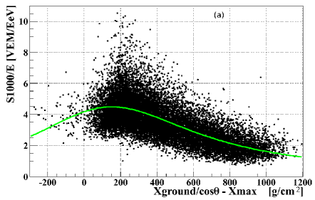
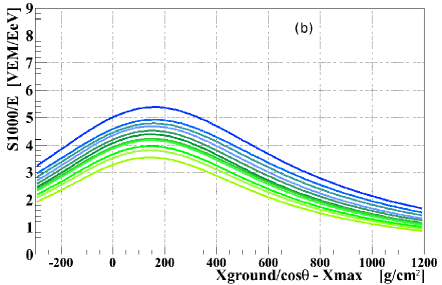
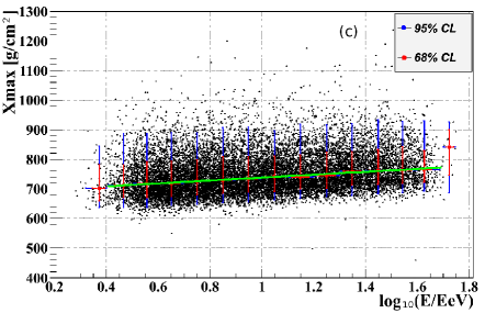
Figure 1: Calibration curves for a mixed sample of iron and proton primaries. The global fit (a) and a different fit for each energy bin (b) are shown. In (b) the curve is lower as energy increases. The evolution of $X_{max}$ as a function of energy is shown in (c). See Sec.3 for details.

4.2 Energy reconstruction

We use the reconstruction sample, which is statistically independent from the calibration, in order to test the method. Given the reconstructed $S(1000)$ and zenith angle of each event, its energy is determined. As an example, Fig. 2 shows the iterative process for a typical event. Solid line represents the global calibration curve while the dashed line is the one used in the last step of the process. It can be seen that the latter is much closer to the real position of the event (red star), improving significantly the energy reconstruction. It was verified that the convergence point is independent of the path followed, so the reconstructed energy does not depend on the initial value used to start the iteration as previously mentioned.

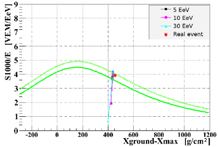
Figure 2: An example of the reconstruction method: first, the global calibration curve (solid line) allows to get a first estimation of the primary energy by iterating between Eq.(6) and itself (process not shown). This energy is used to select a new calibration curve (dashed line) repeating the iterative process with the new curve instead of the global curve. The path followed during the iterative process is shown in the Figure. As can be seen, the convergence point is the same independently of the initial value used to start the iteration (5, 10, 30 EeV) and it is very close to the real position of the event (red star). In this example, the error in the final reconstructed energy is -5$\%$ while it would be larger than +30$\%$ if only the global curve were used.

Fig. 3 shows the error in the reconstructed energy. The two bins at the edges have been rejected for the same reasons as before. Fig. 3.a shows that the energy dependent bias resultant from the use of only the global calibration curve is greatly reduced by employing a set of calibration curves for discrete energies, although a residual error $\leq$1$\%$ still remains. Fig. 3.b also shows the error for proton and iron primaries. The error is almost energy independent for both, each primary taken separately and also for the mixed composition sample. Note also that the error bars, which can be considered as the resolution of the method, are also slightly energy dependent. The energy error distribution for both primaries taken together is approximately Gaussian and the resolution of the method is around 16$\%$, as shown in Fig. 4. In the case of Iron and proton taken separately, the distributions are also nearly Gaussian and the resolution is around 13.5$\%$ and 14.5$\%$ respectively.

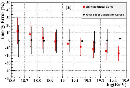
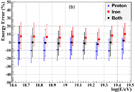
Figure 3: Energy error as a function of primary energy. The points and the error bars are the median and the region of 68$\%$ probability, respectively. (a): Using only a global calibration (red squares) or using a full set of calibration curves (black circles) for a mixture of iron and proton primaries. (b): Proton (blue triangles) and iron (red squares) taken separately and together (black circles) are shown.

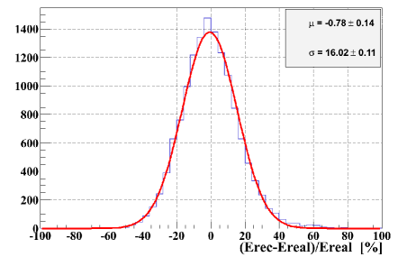
Figure 4: Energy error distribution for the whole sample where equal number of iron and proton primaries in each energy bin are selected.

It is important to note that the method is quite sensitive to the $X_{max}$ vs. $\log(E/\textrm{EeV})$ calibration curve. In fact, if the parameter $q_{0}$ in Eq. (6) is modified by $\pm$10$\%$, an energy error of $\mp$7$\%$ will be produced. This effect is not so important for $q_{1}$, since if it changes $\pm$10$\%$, a negligible error of $\mp$1$\%$ will be obtained.

4.3 Gaussianity of the energy error distributions

Arguably, it is desirable that the errors in energy reconstruction follow a Gaussian distribution. Gaussian errors, for example, are easier to handle and understand when applying deconvolution techniques for determination of the spectrum while assuring that there are no asymmetries or long tails, which further reduces the danger of the limited energy range of the detector and biases associated with a rapidly changing spectral index. An example of these undesirable effects can be seen in Ref. [3].

In case of a Gaussian distribution, the ratio between the high and low parts of the $68\%$ and $95\%$ confidence levels (C.L.) should be 1 since the distribution is symmetric. In addition, the ratio between the $95\%$ and $68\%$ C.L., for both the high and low parts, should be 2 since they represent the values for 2$\sigma$ and 1$\sigma$ respectively. Fig. 5 shows both ratios for the energy error distribution obtained in each energy bin. It has been calculated using the bootstrap technique that consists on resampling the original distribution a large number of times and calculating these ratios for each new sample. The median an $68\%$ C.L. for each ratio are shown in the plots. It can be seen that the error distributions are nearly Gaussian with a very good symmetry and the absence of long tails.

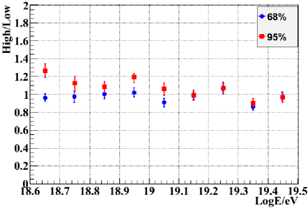
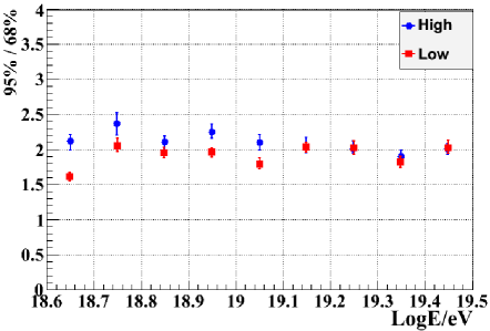
Figure 5: Analysis of the symmetry (top) and the tails (bottom) of the energy error distributions. See text for details.

4.4 Energy bias as a function of the primary composition

We have determined the energy error as a function of the composition of the reconstruction sample. Since the energy error and resolution are almost energy independent for every primary (Fig. 3), we have mixed all the events in this analysis regardless of their energy. We have used $100$ samples with $100$ events each. Proton and Iron primaries are randomly selected such the proton fraction varies from $0$ to $1$ in $0.1$ steps. The energy error as a function of the proton fraction is shown in Fig. 6. The errors are also shown for the case that the calibration curves would have been obtained for each primary separately (we call them proton and iron calibrations in the figure). As expected, the error is negligible if a sample with proton fraction of 0.5 is reconstructed with the calibration from Fig. 1 since equal fraction of proton and iron events were used to get this calibration curves. Note also that if each primary is reconstructed with its own calibration the error is also very close to zero. In the unrealistic scenario that an extremely pure composition sample were reconstructed with the calibration obtained from a mixed composition flux, the absolute value of the incurred error would be $<10\%$.

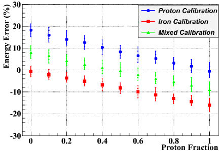
Figure 6: Energy error as a function of the proton fraction of the reconstructed sample using three different sets of calibration curves: the first one obtained with proton showers, the second one from only iron events and, finally, taking both type of primaries together (called mixed here) as shown in Sec. 4.1. The points and the error bars are the median and the confidence levels at $68$ and $95\%$ respectively.

4.5 Different array sizes and geometries

The robustness of the method has been tested by varying the geometry of the array, i.e. the shape of the unitary cell and the distance between detectors.

First, an array with detectors arranged in a squared layout, with a separation of 1200 m is analyzed. Such a geometry is characteristic, for example, of the Telescope Array (TA) observatory. The applicability of the method to a scintillator array as TA is not analyzed here since it would require a different study as a consequence of the different response of scintillators to the muonic part of the shower compared to Cherenkov tanks. As mentioned, this Section focuses on its application to Cherenkov tank arrays with different geometries. The calibration curves and the error in the reconstructed energy are shown in Fig. 7 for a mixed sample. Note that $S(800)$ has been selected as the energy estimator [8]. The error is energy independent and smaller than 1$\%$, while the resolution is $\sim$16$\%$.

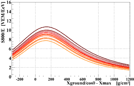
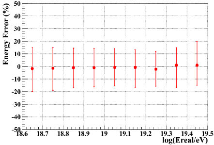
Figure 7: Calibration curves (top) and error in the reconstructed energy (bottom) for the Telescope Array geometry. The points and the error bars are the median and the confidence levels at 68$\%$.

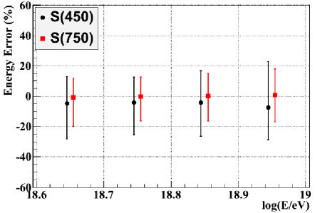
Figure 8: Error in the reconstructed energy in case of a triangular array whose distance between detectors is 750 m. Two different energy estimators are used, $S(450)$ and $S(750)$. Points and error bars are the median and 68$\%$ confidence levels. See text for details.

Second, a smaller triangular array is considered. A geometry representative of the Auger Infill is selected, i.e. a triangular grid with 750 m spacing between detectors. The Infill is essentially designed to explore the region below the ankle and to reach full efficiency above $\sim$10^17.6 eV [29]. The fraction of saturated events is very large above 10¹⁹ eV, so we only analyzed here the interval from 10^18.6 to 10¹⁹ eV. In the energy range of the experiment, the average optimum distance is $r_{0}=450$ m, so $S(450)$ is selected as the energy estimator [29]. Then, the error in the reconstructed energy is around -5$\%$ as shown in Fig. 8. The error comes from the lack of events close to the maximum of the calibration curves which, as mentioned previously, is a key point in order to get a reliable fit and calibration. Since the optimum distance increases with primary energy [3], the average r₀ is higher for the energy range analyzed here. Thus, the error could be minimized if a larger $r_{0}$ were selected. For example, using $S(750)$ the error would be negligible (Fig. 8).

5 Conclusions

An iterative method, previously developed to infer the primary energy of photon-induced showers in pure surface arrays, has been modified to be applicable to hadron-initiated showers and tested assuming a hybrid experiment. The method is based on a set of calibration curves that relate the surface energy estimator, $S(r_{0})$, and the depth of maximum development of the shower, $X_{max}$, thanks to hybrid events. In pure surface arrays, a similar procedure could be performed but the calibration should rely on Monte Carlo (MC) parametrizations. However, it is important to note that MC parametrizations could be affected by the fact that the simulations do not reproduce properly the available experimental data [30], a major advantage of the hybrid experiments.

The original method is based on the well-known universality of the electromagnetic component of the showers and the small number of muons produced in the development of photon cascades. However, the significant fraction of the muon component for hadron-initiated showers, breaks the universality and makes necessary to implement a full set of calibration curves depending on the primary energy.

Our own simulation program of the detector response has been used. Shower to shower fluctuations and reconstruction uncertainties (core position, LDF fit and signal fluctuations) have been implemented. Primary energy and zenith angles go from 10^18.5 to 10^19.6 eV and from 0 to 60 degrees respectively. Several array geometries varying the shape of the unitary cell (triangular and square) and the distance between detectors (1500, 1200 and 750 m) have been studied. Considering a mixed sample of proton and iron primaries, the energy is determined with a negligible error and resolution around 16$\%$ in the full energy range analyzed.

Obviously, the same composition is expected for hybrid (used for the calibration) and pure surface events, so the energy of the latter could be determined with error close to zero. However, in the extreme scenario that the reconstructed events present a pure composition, the energy error could achieve $\sim$10$\%$. This could be considered as the maximum uncertainty of the method due to the unknown composition of the primary flux.

The energy error distributions are nearly Gaussian, an important point to get a more reliable reconstruction of the shape and position of rapidly varying spectral features since they are easier to manage when applying deconvolution techniques in the spectrum determination.

6 Acknowledgments

All the authors have greatly benefited from their participation in the Pierre Auger Collaboration and its profitable scientific atmosphere. Extensive numerical simulations were made possible by the use of the UNAM super-cluster Kanbalam, computational resources at ICN-UNAM and the UAH-SPAS cluster at the Universidad de Alcalá. We want to thank J. A. Morales de los Ríos for the maintenance of the UAH-SPAS cluster. LdP and MDRF also thank to ITeDA-CNEA for its hospitality during their stay. ADS is member of the Carrera del Investigador Científico of CONICET, Argentina.

We also thank the support of the MICINN Consolider-Ingenio 2010 Programme under grant MULTIDARK CSD2009-00064, ASTROMADRID S2009/ESP-1496, and EPLANET FP7-PEOPLE-2009-IRSES. This work is partially supported by grant PAPIIT 107413, several grants from CONACyT either directly or through the Network of High Energy Physics (Red FAE), CONICET PIP 114-201101-00360 and ANPCyT PICT-2011-2223, Argentina.

References

- [1] The Pierre Auger Collaboration. Nucl. Instrum. Meth. A, 620 (2010) 227-251.
- [2] D. Newton et al. Astroparticle Physics, 26 (2007) 414-419.
- [3] G. Ros et al. Nucl. Instrum. Meth. A, 608 (2009) 454-463.
- [4] The Pierre Auger Collaboration. Nucl. Instrum. and Meth. A, 523 (2004) 50-95.
- [5] H. Kawai et al. Nucl. Phys. Proc. Suppl. B, 175-176 (2008) 221-226.
- [6] Pierre Auger Collaboration. 33rd International Cosmic Ray Conference, Rio de Janeiro, Brasil, 2013. arXiv:1307.5059 (see contribution by A. Schulz).
- [7] The Pierre Auger Collaboration, Physics Letters B, 685 (2010) 239–246.
- [8] T. Abu-Zayyad et al. (Telescope Array Collaboration). Astrophys. J., 768, L1 (2013).
- [9] M. Ave et al. Phys. Rev. D, 65, 063007 (2002).
- [10] K. Shinozaki et al. Astrophys. J. 571, L117 (2002).
- [11] M. Risse et al. Phys. Rev. Lett. 95, 171102 (2005).
- [12] T. Abu-Zayyad et al. (Telescope Array Collaboration) Phys. Rev. D, 88, 112005 (2013).
- [13] Pierre Auger Collaboration. Astroparticle Physics, 29 (2008) 243-256.
- [14] P. Billoir, C. Roucelle, J.C. Hamilton. arXiv:astro-ph/0701583 (2007).
- [15] S. Lafebre et al. Astroparticle Physics, Vol. 31, Issue 3 (2009) 243-254.
- [16] W. D. Apel et al. Astroparticle Physics, 29 (2008) 412-419.
- [17] F. Schmidt et al. Proceedings of the 30th International Cosmic Ray Conference, Merida, Mexico, 2007. arXiv:0706.1990.
- [18] S. Sciutto. arXiv:astro-ph/9911331 (1999).
- [19] S. Ostapchenko, Nucl. Phys. Proc. Suppl. B, 151 (2006) 143.
- [20] G. Ros et al., Astroparticle Physics, 35 (2011) 140.
- [21] G. Ros et al., Astroparticle Physics, 47 (2013) 10-17.
- [22] T. C. Schmidt, I. C. Maris and M. Roth. GAP Note 2007-106. Pierre Auger Collaboration Internal Document (2007).
- [23] I. C. Maris. PhD Thesis. (2008). Available at http://digbib.ubka.uni-karlsruhe.de/volltexte/documents/697773.
- [24] M. Ave for the Pierre Auger Collaboration. 29th International Cosmic Ray Conference, Merida, Mexico, 2007. arxiv:astro-ph:0709.2125.
- [25] Pierre Auger Collaboration. 33rd International Cosmic Ray Conference, Rio de Janeiro, Brasil, 2013. arXiv:1307.5059 (see contribution by D. Veberič).
- [26] Pierre Auger Collaboration. Nucl. Phys. Proc. Suppl. 190 (2009) 20-25.
- [27] T. Abu-Zayyad et al. (Telescope Array Collaboration). arXiv:1305.7273v1 (2013).
- [28] E. Barcikowski, et al. for the HiRes, Pierre Auger, Telescope Array and Yakutsk Collaborations. EPJ Web of Conference 53, 01006 (2013).
- [29] Pierre Auger Collaboration. 33rd International Cosmic Ray Conference, Rio de Janeiro, Brasil, 2013. arXiv:1307.5059 (see contribution by D. Ravignani).
- [30] Pierre Auger Collaboration. 33rd International Cosmic Ray Conference, Rio de Janeiro, Brasil, 2013. arXiv:1307.5059 (see contribution by B. Kégl).