Isotropic matroids II: Circle graphs

Abstract

We present several characterizations of circle graphs, which follow from Bouchet’s circle graph obstructions theorem.

Keywords: 4-regular graph, circle graph, delta-matroid, Euler circuit, interlacement, isotropic system, local equivalence, matroid, multimatroid

1 Introduction

Let $F$ be a 4-regular graph and let $C$ be an Euler system of $F$, i.e., a set that includes precisely one Euler circuit of each connected component of $F$. Then the interlacement graph $\mathcal{I}(C)$ of $C$ is the simple graph with vertex-set equal to the set $V(F)$ of vertices of $F$, in which $v_{i}$ and $v_{j}$ are adjacent if and only if they are interlaced with respect to $C$, i.e., they appear in the order $v_{i}\ldots v_{j}\ldots v_{i}\ldots v_{j}$ or $v_{j}\ldots v_{i}\ldots v_{j}\ldots v_{i}$ on one of the circuits of $C$. A simple graph that arises from this construction is called a circle graph.

The idea of interlacement is almost 100 years old, as it was used by Brahana in defining his separation matrix [14]. Interlacement graphs were first discussed by Zelinka [44], who credited the idea to Kotzig. But circle graphs did not become well known until the 1970s, when Cohn and Lempel [20] and Even and Itai [22] used them to analyze permutations, and Bouchet [1] and Read and Rosenstiehl [35] used them to study Gauss’ problem of characterizing generic self-intersecting curves in the plane. Circle graphs were studied intensively during the next few decades. Among the notable results of this intensive study are polynomial-time recognition algorithms due to Bouchet [3], Gioan, Paul, Tedder and Corneil [27], Naji [32] and Spinrad [36]. In recent years, interest in 4-regular graphs (and indirectly on circle graphs) has also focused on their appearance as medials of graphs imbedded on surfaces [21].

See Figure 1 for an example. On the left is a 4-regular graph, with an indicated Euler circuit. To trace the Euler circuit just walk along the edges, making sure to preserve the dash style (dashed or plain) when traversing a vertex; the dash style will sometimes change in the middle of an edge, though. On the right is the resulting interlacement graph.

Figure 1: An Euler circuit and its interlacement graph.

If $v\in V(F)$, then the $\kappa$-transform $C\ast v$ is the Euler system obtained from $C$ by reversing one of the $v$-to-$v$ walks within the circuit of $C$ incident at $v$. As we do not distinguish between circuits that differ only in starting point or orientation, the same Euler system will result no matter which of the two $v$-to-$v$ walks is reversed. The $\kappa$-transformations were introduced by Kotzig [30], who proved the fundamental theorem that any two Euler systems of $F$ are connected through some finite sequence of $\kappa$-transformations. As noted by Read and Rosenstiehl [35], the interlacement graph $\mathcal{I}(C\ast v)$ is the simple local complement $\mathcal{I}(C)_{s}^{v}$, the simple graph obtained from $\mathcal{I}(C)$ by reversing all adjacencies among neighbors of $v$. Simple graphs that can be obtained from each other through local complementations are said to be locally equivalent, and an induced subgraph of a simple graph locally equivalent to $G$ is called a vertex-minor of $G$.

We use the subscript $s$ to distinguish simple local complementation from a closely related operation $G\mapsto G_{ns}^{v}$ on looped simple graphs, which we call non-simple local complementation. This operation reverses the adjacencies between every pair of vertices in the open neighborhood $N(v)$ and complements the loop status of every vertex in $N(v)$. Looped simple graphs that can be obtained from each other through non-simple local complementations and loop complementations are said to be locally equivalent. In particular, $G$ is a circle graph if and only if every graph obtained from $G$ using loop complementations is also a circle graph; consequently loops are irrelevant to characterizations of circle graphs, and most results regarding circle graphs are stated for simple graphs.

Bouchet [7] gave a famous characterization of circle graphs: a simple graph is a circle graph if and only if none of the three graphs pictured in Figure 2 is a vertex-minor. We refer to this famous result as Bouchet’s theorem. Bouchet’s theorem resembles several well-known forbidden minors characterizations of matroid classes: for instance a matroid is binary iff $U_{2,4}$ is not a minor, a binary matroid is regular iff neither $F_{7}$ nor $F_{7}^{\ast}$ is a minor, and a regular matroid is graphic iff neither $M^{\ast}(K_{5})$ nor $M^{\ast}(K_{3,3})$ is a minor. But Bouchet’s theorem involves induced subgraphs rather than matroid minors, and including local equivalence makes Bouchet’s theorem seem more complicated than the classic matroid results. The present paper was initially motivated by a couple of questions suggested by this resemblance: Can Bouchet’s theorem be rephrased to characterize circle graphs using matroids? If so, is it possible to state such a characterization without mentioning local equivalence? It turns out that both answers are “yes”; we present several such characterizations below. In the process of explaining them we also obtain other circle graph characterizations, some of which involve local equivalence and do not explicitly mention matroids.

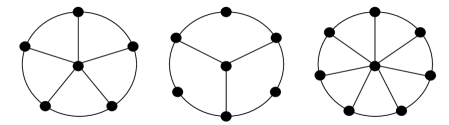
Figure 2: Bouchet’s circle graph obstructions: $W_{5}$, $BW_{3}$ and $W_{7}$.

To state these characterizations, we introduce some terminology. First, we note that we follow the convention that if $X$ and $Y$ are finite sets then an $X\times Y$ matrix has rows indexed by elements of $X$ and columns indexed by elements of $Y$. If $G$ is a simple graph then we consider the adjacency matrix $A=A(G)$ and the $n\times n$ identity matrix $I$ as $V(G)\times V(G)$ matrices over $GF(2)$. Let $IAS(G)$ be the matrix

$$IAS(G)=\begin{pmatrix}I&A&I+A\end{pmatrix}\text{.}$$

The rows of $IAS(G)$ inherit indices in $V(G)$ from the rows of $I$ and $A(G)$. Notation for the columns of $IAS(G)$ follows this scheme: the $v$ column of $I$ is designated $\phi_{G}(v)$, the $v$ column of $A$ is designated $\chi_{G}(v)$, and the $v$ column of $I+A$ is designated $\psi_{G}(v)$. The set $\{\phi_{G}(v),\chi_{G}(v),\psi_{G}(v)\mid v\in V(G)\}$ is denoted $W(G)$, and the binary matroid on $W(G)$ represented by $IAS(G)$ is the isotropic matroid of $G$, $M[IAS(G)]$ [40]. If $v\in V(G)$ then the subset $\{\phi_{G}(v),\chi_{G}(v),\psi_{G}(v)\}$ of $W(G)$ is the vertex triple corresponding to $v$. Notice that the three columns of $IAS(G)$ corresponding to a vertex triple sum to $0$. If $v$ is not isolated then each of these columns has a nonzero entry, so the vertex triple is a circuit of $M[IAS(G)]$. If $v$ is isolated, instead, then $\{\chi_{G}(v)\}$ and $\{\phi_{G}(v),\psi_{G}(v)\}$ are separate circuits of $M[IAS(G)]$. A transversal of $W(G)$ is a subset that includes precisely one element of each vertex triple, and a subset of a transversal is a subtransversal. A transverse matroid of $G$ is a matroid obtained by restricting $M[IAS(G)]$ to a transversal. (We use “transverse matroid” to avoid confusion with transversal matroids.) A transverse circuit of $G$ is a circuit of a transverse matroid of $G$.

The general theory of isotropic matroids is presented in [19] and [40]. Part of this theory is the following result:

Theorem 1.

([19]) Let $G$ and $H$ be simple graphs. Then any one of the following conditions implies the others:

1. $G$ and $H$ are locally equivalent, up to isomorphism.

2. The isotropic matroids of $G$ and $H$ are isomorphic.

3. There is a bijection between $W(G)$ and $W(H)$, which defines isomorphisms between the transverse matroids of $G$ and those of $H$.

4. There is a bijection between $W(G)$ and $W(H)$, under which vertex triples and transverse circuits of $G$ and $H$ correspond.

In particular, if $G$ and $H$ are locally equivalent then each sequence of local complementations that may be used to obtain $H$ from $G$ yields an induced isomorphism $M[IAS(G)]\rightarrow M[IAS(H)]$, which is compatible with the partitions of $W(G)$ and $W(H)$ into vertex triples.

All the interlacement graphs of Euler systems of a particular 4-regular graph $F$ are locally equivalent (up to isomorphism); it follows that the class of circle graphs is closed under local complementation. Theorem 1 then implies that there must be matroidal characterizations of circle graphs using their isotropic matroids, their transverse circuits and their transverse matroids. Circle graph characterizations involving isotropic matroids are complicated by the fact that the class of isotropic matroids is not closed under matroid minors. (The order of an isotropic matroid is divisible by 3, so deleting or contracting an element of an isotropic matroid cannot yield another isotropic matroid.) In order to derive such characterizations we need a special minor operation that is appropriate for isotropic matroids.

Definition 2.

Let $G$ be a looped simple graph, let $S$ be a subtransversal of $W(G)$, and let $S^{\prime}$ contain the other $2\left|S\right|$ elements of $W(G)$ that correspond to the same vertices of $G$ as elements of $S$. Then the isotropic minor of $G$ obtained by contracting $S$ is the matroid

$$(M[IAS(G)]/S)-S^{\prime}.$$

We use the term isotropic minor because the definition is consistent with Bouchet’s definitions of minors of isotropic systems [2] and multimatroids [9].

Theorem 3.

([40]) The isotropic minors of $G$ are precisely the isotropic matroids of vertex-minors of $G$.

Bouchet’s theorem now leads directly to a characterization of circle graphs by excluded isotropic minors.

Theorem 4.

Let $G$ be a simple graph. Then $G$ is a circle graph if, and only if, the isotropic matroids of $W_{5}$, $BW_{3}$ and $W_{7}$ are not isotropic minors of $G$.

It follows that we may try to gain insight into the special characteristics of circle graphs by contrasting their isotropic minors of size $\leq 24$ with the isotropic matroids of $W_{5}$, $BW_{3}$ and $W_{7}$. Formulating and verifying these contrasts is facilitated by the following four theorems, which show that isotropic matroids reflect important structural properties of graphs.

Theorem 5.

Let $G$ be an interlacement graph of an Euler system of a 4-regular graph $F$, and let $k$ be a positive integer. If $F$ has a $k$-circuit then $G$ has a transverse circuit of size $\leq k$.

Theorem 5 is discussed in Section 4. The next three theorems are discussed in [19].

Theorem 6.

([19]) Let $G$ be a simple graph, and let $k$ be a positive integer. Then $G$ has a transverse $k$-circuit if and only if some graph locally equivalent to $G$ has a vertex of degree $k-1$.

Theorem 7.

([19]) Let $G$ be a simple graph, and let $k_{1},k_{2}$ be positive integers. Then $G$ is locally equivalent to a graph with adjacent vertices of degrees $k_{1}-1$ and $k_{2}-1$ if and only if $G$ has transverse circuits $\gamma_{1},\gamma_{2}$ such that $\left|\gamma_{i}\right|=k_{i}$, the largest subtransversals contained in $\gamma_{1}\cup\gamma_{2}$ are of cardinality $\left|\gamma_{1}\cup\gamma_{2}\right|-2$, and two of these largest subtransversals are independent sets of $M[IAS(G)]$.

Theorem 8.

([19]) Let $G$ be a simple graph, and let $k_{1},k_{2}$ be positive integers. Then these two conditions are equivalent:

• $G$ is locally equivalent to a graph with nonadjacent vertices of degrees $k_{1}-1$ and $k_{2}-1$, which share no neighbor.

• $G$ has disjoint transverse circuits $\gamma_{1},\gamma_{2}$ such that $\left|\gamma_{i}\right|=k_{i}$ and $\gamma_{1}\cup\gamma_{2}$ is a subtransversal, which contains no other circuit.

Here is an illustration of the usefulness of these properties. It is easy to see that up to isomorphism, there are only two simple 4-regular graphs with $\leq 6$ vertices: one is $K_{5}$ and the other is obtained from $K_{6}$ by removing the edges of a perfect matching. Each of these graphs contains several 3-circuits. A non-simple 4-regular graph must contain a 1-circuit or a 2-circuit, of course, so Theorem 5 tells us that every circle graph with $\leq 6$ vertices has a transverse circuit of size $\leq 3$. According to Theorem 6, this is equivalent to saying that every circle graph with $\leq 6$ vertices is locally equivalent to a graph with a vertex of degree $\leq 2$. Inspecting the matrix $IAS(W_{5})$, it is not hard to see that the only circuits of size $\leq 3$ in $M[IAS(W_{5})]$ are vertex triples; the smallest transverse circuits are of size 4. It follows from Theorem 6 that no simple graph locally equivalent to $W_{5}$ has a vertex of degree $\leq 2$. This is enough to verify the following.

Corollary 9.

Let $G$ be a simple graph with $\leq 6$ vertices. Then any one of the following properties implies the others.

1. $G$ is a circle graph.

2. $G$ has a transverse circuit of size $\leq 3$.

3. $G$ is locally equivalent to a graph with a vertex of degree $\leq 2$.

Further analysis leads to several characterizations of larger circle graphs. For instance, here is a characterization that involves both isotropic matroids and transverse matroids.

Theorem 10.

A simple graph $G$ is a circle graph if and only if $G$ satisfies all of the following conditions.

1. Every transverse matroid of $G$ is cographic.

2. Every isotropic minor of $G$ of size $<24$ has a loop or a pair of intersecting 3-circuits.

3. Suppose an isotropic minor $M$ of $G$ of size $24$ has no loop and no pair of intersecting 3-circuits. Then every transverse matroid of $M$ that contains two disjoint circuits also contains other circuits.

The three conditions of Theorem 10 correspond directly to the three obstructions of Bouchet’s theorem: condition 1 excludes $BW_{3}$, condition 2 excludes $W_{5}$, and condition 3 excludes $W_{7}$. By the way, we state condition 2 this way only for variety. As vertex triples are dependent sets, it is not hard to see that an isotropic matroid has a transverse circuit of size $\leq 3$ if and only if it has a loop or a pair of intersecting 3-circuits. Details of the argument appear in the proof of Corollary 41.

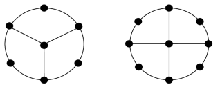
Figure 3: $BW_{3}$ and $BW_{4}$.

Condition 1 is of particular interest for several reasons. One reason is simply that the cographic property is more familiar than the small-circuit properties mentioned in conditions 2 and 3. Another reason is that it is possible to explicitly construct the graphs whose cocycle matroids are the transverse matroids of a circle graph; see Section 4 for details. Yet another reason is that, as we show in Section 8, condition 1 suffices to characterize a special type of circle graph.

Theorem 11.

Let $G$ be a simple graph that is locally equivalent to a bipartite graph. Then any one of the following properties implies the others.

1. $G$ is a circle graph.

2. Every transverse matroid of $G$ is cographic.

3. Neither graph of Figure 3 is a vertex-minor of $G$.

Bipartite circle graphs are important for two reasons. One reason is that bipartite circle graphs correspond to planar 4-regular graphs, and the other reason is that all circle graphs are vertex-minors of bipartite circle graphs. Details are given in Sections 8 and 9, along with some results about the connection between the crossing number of a 4-regular graph and the matroidal properties of its associated circle graphs.

Returning to the general case, note that conditions 2 and 3 of Theorem 10 indicate characteristic properties of the transverse circuits of small isotropic minors of circle graphs. Theorems 6 – 8 tell us that these properties are related to the distribution of low-degree vertices in small vertex-minors of circle graphs.

Theorem 12.

Let $G$ be a simple graph, and let $\mathcal{VM}_{8}(G)$ denote the set of graphs with 8 or fewer vertices, which are vertex-minors of $G$. Then $G$ is a circle graph if and only if every $H\in\mathcal{VM}_{8}(G)$ satisfies at least one of the following conditions.

1. Some graph locally equivalent to $H$ has a vertex of degree $0$ or $1$.

2. Some graph locally equivalent to $H$ has a pair of adjacent degree-$2$ vertices.

3. Every graph locally equivalent to $H$ has a vertex of degree $5$.

As every $H\in\mathcal{VM}_{8}(G)$ must satisfy one of the conditions, condition 3 is logically equivalent to the simpler requirement that $H$ itself must have a vertex of degree 5. Condition 3 may also be replaced by the weaker requirement that there be a vertex of degree $\geq 4$, because $W_{5}$ and $W_{7}$ are both locally equivalent to 3-regular graphs. See Figure 4.

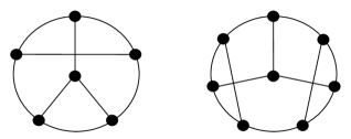
Figure 4: Cubic graphs locally equivalent to $W_{5}$ and $W_{7}$.

Several other circle graph characterizations are presented in Sections 5–9. Although the details differ, most are variations on the theme “circle graphs have vertex-minors with distinctive distributions of small transverse circuits.”

Before deriving these matroidal characterizations of circle graphs, we discuss a different kind of structural characterization of circle graphs, using delta-matroids. It is shown in [25] that a variant of unimodularity called principal unimodularity precisely corresponds to representability of a delta-matroid $D$ over every field. This specializes to the usual notion of unimodularity in case $D$ is a matroid. In this way, this result generalizes the well-known result that unimodular representations of matroids correspond precisely to matroids representable over every field. It has been shown by Bouchet (see Geelen’s PhD thesis [25]) that circle graphs are precisely the graphs $G$ such that for every graph $G^{\prime}$ locally equivalent to $G$, $G^{\prime}$ allows for a principal unimodular representation. In Section 2 we reformulate this characterization in terms of binary delta-matroids. Using this characterization, we provide in Section 3 a characterization of isotropic matroids of circle graphs in terms of principal unimodularity, but without mentioning local equivalence. The techniques used in Section 3 are from multimatroid theory [8] and it is essentially shown that the natural $3$-matroid generalization of principal unimodularity precisely characterizes isotropic matroids of circle graphs.

More specifically, for an isotropic matroid $M[IAS(G)]$ and transversal $T$, we say that $M[IAS(G)]-T$ is tight if for every independent subtransversal $S$ disjoint from $T$ with $|S|=|V(G)|-1$ there is an element $x\in W(G)\setminus T$ such that $S\cup\{x\}$ is a dependent subtransversal. Also, we say that $M[IAS(G)]-T$ is t-regular (short for “transversal-regular”) if $M[IAS(G)]-T$ has a representation $E$ such that for each transversal $T^{\prime}$ disjoint from $T$, the determinant of the matrix obtained from $E$ by restricting to the columns of $T^{\prime}$ is equal to $0$, $1$, or $-1$.

We show the following (cf. Theorem 25).

Theorem 13.

Let $G$ be a simple graph. Then $G$ is a circle graph if and only if for all transversals $T$, if $M[IAS(G)]-T$ is tight, then $M[IAS(G)]-T$ is t-regular.

2 Characterizing circle graphs by delta-matroid regularity

In this section we recall a characterization of circle graphs using the notion of regularity for delta-matroids and multimatroids.

2.1 Delta-matroids

A set system (over $V$) is a tuple $D=(V,S)$ such that $S\subseteq 2^{V}$ is a set of subsets of a ground set $V$ of $D$. For notational simplicity we write $X\in D$ to denote $X\in S$. We say that $D$ is empty if $S=\varnothing$. A delta-matroid $D$ is a nonempty set system $(V,S)$ that satisfies the following property: for all $X,Y\in S$ and $x\in X\mathop{\mathrm{\Delta}}Y$, there is a $y\in X\mathop{\mathrm{\Delta}}Y$ (we allow $y=x$) such that $X\mathop{\mathrm{\Delta}}\{x,y\}\in S$ [4]. It turns out that if all sets of $D$ have the same cardinality, then $D$ is a matroid represented by its bases [4]. In this way, a delta-matroid can be viewed as a generalization of the notion of matroid. A delta-matroid $D$ is called even if the cardinalities of the sets of $D$ have equal parity. For $X\subseteq V$, we define the twist of $D$ by $X$ as the set system $D\ast X=(V,S^{\prime})$ with $S^{\prime}=\{X\mathop{\mathrm{\Delta}}Y\mid Y\in S\}$. It turns out that $D\ast X$ is an (even) delta-matroid if and only if $D$ is an (even) delta-matroid.

2.2 Representable and regular delta-matroids

For finite sets $X$ and $Y$, an $X\times Y$-matrix $A$ is a matrix where the rows and columns of $A$ are indexed by $X$ and $Y$, respectively, and are not ordered. If $W\subseteq X$ and $W\subseteq Y$, then $A[W]$ denotes the $W\times W$-matrix obtained from $A$ by removing the entries outside $W$. We now fix a finite set $V$. A $V\times V$-matrix $A$ over some field $\mathbb{F}$ is said to be skew-symmetric if $-A^{T}=A$ (note that we allow nonzero diagonal entries in case $\mathbb{F}$ is of characteristic $2$). If $A$ is skew-symmetric, then $\mathcal{D}_{A}=(V,S)$ with $S=\{X\mid A[X]\mbox{ is nonsingular}\}$ is a delta-matroid [4]. For a skew-symmetric $V\times V$-matrix $A$ over $\mathbb{F}$, $\mathcal{D}_{A}$ is even if and only if all diagonal entries of $A$ are zero. A delta-matroid $D$ is said to be representable over $\mathbb{F}$ if there is a skew-symmetric $V\times V$-matrix $A$ over $\mathbb{F}$ such that $D=\mathcal{D}_{A}\ast X$ for some $X\subseteq V$. This notion of representability for delta-matroids generalizes the notion of representability for matroids: a matroid $M$ is representable over $\mathbb{F}$ in the standard matroid sense if and only if $M$ is representable over $\mathbb{F}$ in the delta-matroid sense. Indeed, if $M$ is representable by a matrix

$$\bordermatrix{&X&Y\cr X&I&E}$$

in standard form, then one may verify that the delta-matroid $\mathcal{D}_{A}$ corresponding to skew-symmetric matrix $V\times V$-matrix

$$A=\bordermatrix{&X&Y\cr X&0&E\cr Y&-E^{\text{T}}&0\cr}$$

is such that $\mathcal{D}_{A}\ast X=M$. The converse also holds [4].

A $V\times V$-matrix $A$ over $\mathbb{R}$ is said to be principally unimodular if $\det(A[X])\in\{0,1,-1\}$ for all $X\subseteq V$. (In particular, if $A$ is principally unimodular, then each entry of $A$ is equal to $0$, $1$, or $-1$.) We say that $D$ is regular if $D$ is representable by a skew-symmetric principally unimodular matrix over $\mathbb{R}$. The following result is shown by Geelen [25].

Theorem 14 ([25]).

Let $D$ be an even delta-matroid. Then the following statements are equivalent.

1. $D$ is regular,

2. $D$ is representable over every field, and

3. $D$ is representable over both $GF(2)$ and $GF(3)$.

The notion of regularity for delta-matroids generalizes the notion of regularity for matroids. Recall that a matroid $M$ is called regular if $M$ is representable by a totally unimodular matrix over $\mathbb{R}$, where a matrix $B$ over $\mathbb{R}$ is said to be totally unimodular if the determinant of every submatrix of $B$ is equal to $0$, $1$, or $-1$. We may assume that $B$ is in standard form $(I\quad E)$. Now, it is easy to verify that

$$\bordermatrix{&X&Y\cr X&I&E}$$

is totally unimodular if and only if the skew-symmetric matrix $V\times V$-matrix

$$A=\bordermatrix{&X&Y\cr X&0&E\cr Y&-E^{\text{T}}&0\cr}$$

with $V=X\cup Y$ is principally unimodular [12].

If $A$ is a skew-symmetric matrix over $GF(2)$ (equivalently, $A$ is symmetric over $GF(2)$), then $\mathcal{D}_{A}$ uniquely determines $A$ [13]. Indeed, for $v\in V$, $A[\{v\}]=1$ if and only if $\{v\}\in\mathcal{D}_{A}$. Moreover, for $v,w\in V$ with $v\neq w$, we have $A[\{v,w\}]=1$ if and only if we have either $(\{v,w\}\in\mathcal{D}_{A})\land((\{v\}\notin\mathcal{D}_{A})\lor(\{w\}\notin\mathcal{D}_{A})$ or $(\{v,w\}\notin\mathcal{D}_{A})\land(\{v\}\in\mathcal{D}_{A})\land(\{w\}\in\mathcal{D}_{A})$. We say that $D$ is binary if $D$ is representable over $GF(2)$.

2.3 Eulerian delta-matroids

A delta-matroid $D$ is said to be Eulerian if $D=\mathcal{D}_{A(G)}*X$ where $G$ is a circle graph and $X\subseteq V(G)$ [25]. For notational convenience, this definition is slightly different from [25] as there it is required that $X=\varnothing$. The next lemma shows that this difference is not essential.

Lemma 15.

Let $G$ be a simple graph. Then $G$ is a circle graph if and only if $\mathcal{D}_{A(G)}$ is Eulerian.

Proof.

The only if direction is trivial. To prove the converse, let $D=\mathcal{D}_{A(G)}$ be Eulerian. Then $D*X=\mathcal{D}_{A(G^{\prime})}$ for some circle graph $G^{\prime}$. Hence, $\mathcal{D}_{A(G)}=\mathcal{D}_{A(G^{\prime})}*X$. It is shown in [4] that this implies that $G$ is locally equivalent to $G^{\prime}$. By Theorems 1 and 4, $G$ is a circle graph as well. ∎

It follows from de Fraysseix [24] that Eulerian delta-matroids are a generalization of planar matroids (i.e., cycle matroids of planar graphs); see also [25, Theorem 4.16].

Theorem 16 ([24]).

Let $M$ be a matroid. Then $M$ is planar if and only if $M$ is an Eulerian delta-matroid.

Since $\mathcal{D}_{A}$ uniquely determines $A$, a characterization of Eulerian delta-matroids directly implies a characterization of circle graphs. The following characterization of Eulerian delta-matroids is from [25].

Theorem 17 ([25]).

Let $D$ be an even binary delta-matroid, i.e., $D=\mathcal{D}_{A(G)}*X$ for some simple graph $G$ and $X\subseteq V(G)$. Then $D$ is Eulerian if and only if, for every graph $G^{\prime}$ locally equivalent to $G$, $\mathcal{D}_{A(G^{\prime})}$ is regular.

In particular, every Eulerian delta-matroid is regular. The converse does not hold: any regular matroid $M$ that is not planar is a counterexample by Theorem 16. So, e.g., the cycle matroids of $K_{3,3}$ and $K_{5}$ are regular, but they are not Eulerian delta-matroids.

Since $\mathcal{D}_{A(G)}$ uniquely determines $G$, it is natural to formulate the notion of local equivalence for binary delta-matroids. For this we require an additional operation on delta-matroids. For a delta-matroid $D$ over $V$ and $X\subseteq V$, loop complementation of $D$ by $X$, denoted by $D+X$, is defined by $Y\in D+X$ if and only if there are an odd number of $Z\in D$ with $(Y-X)\subseteq Z\subseteq Y$. In general $D+X$ need not be a delta-matroid, but it turns out that the family of binary delta-matroids is closed under loop complementation [15, Section 5].

We now use loop complementation to reformulate Theorem 17.

Theorem 18.

Let $D$ be an even binary delta-matroid over $V$. Then the following statements are equivalent.

1. $D$ is Eulerian,

2. for all $X\subseteq Y\subseteq V$ with $D*X+Y$ even, we have that $D*X+Y$ is regular,

3. every even delta-matroid obtainable from $D$ by applying a sequence of $+$ and $*$ operations is regular.

Proof.

Statement 3 implies statement 2 directly. For the converse, recall that it is shown in [15, Theorem 12] that any delta-matroid $D^{\prime}$ obtainable from $D$ by applying a sequence of $+$ and $*$ is of the form $D*X+Y*Z$ with $X\subseteq Y\subseteq V$ and $Z\subseteq V$. As twists preserve both evenness and regularity, $D*X+Y*Z$ is even (regular) if and only if $D*X+Y$ is even (regular). Hence the last two statements are equivalent.

It is shown in [15, Theorem 27] that for simple graphs $G$ and $G^{\prime}$, $G^{\prime}$ is locally equivalent to $G$ if and only if $\mathcal{D}_{A(G^{\prime})}$ can be obtained from $\mathcal{D}_{A(G)}$ by applying a sequence of $+$ and $*$ operations. By Theorem 17, we obtain that statement 3 implies that $D$ is Eulerian. Conversely, let $D$ be Eulerian. Then $D=\mathcal{D}_{A(G)}*X$ for some simple graph $G$ and $X\subseteq V(G)$. Let $\varphi$ be a sequence of $+$ and $*$ operations such that $D\varphi$ is even. Then $(\mathcal{D}_{A(G)}*X)\varphi$ is even. Let $Y\in(\mathcal{D}_{A(G)}*X)\varphi$. Then $(\mathcal{D}_{A(G)}*X)\varphi*Y$ contains the empty set and so it is equal to $\mathcal{D}_{A(G^{\prime})}$ for some graph $G^{\prime}$ by [16, Proof of Theorem 8.2]. Hence $G^{\prime}$ is locally equivalent to $G$ and so $\mathcal{D}_{A(G^{\prime})}$ is regular (as $D$ is Eulerian). Thus $D\varphi=\mathcal{D}_{A(G^{\prime})}*Y$ is regular and so statement 3 holds. ∎

Corollary 19.

Let $M$ be a binary matroid. Then $M$ is planar if and only if every even delta-matroid obtainable from $D$ by applying a sequence of $+$ and $*$ operations is regular.

3 Characterizing circle graphs by multimatroid regularity

In this section we reformulate Theorem 17 in terms of isotropic matroids.

3.1 Sheltering matroids

First we recall some notions and notation for the theory of multimatroids [8]. Let $\Omega$ be a partition of a finite set $U$. A set $T\subseteq U$ is called a transversal (subtransversal, respectively) of $\Omega$ if $|T\cap\omega|=1$ ($|T\cap\omega|\leq 1$, respectively) for all $\omega\in\Omega$. We denote the set of transversals of $\Omega$ by $\mathcal{T}(\Omega)$ and the set of subtransversals of $\Omega$ by $\mathcal{S}(\Omega)$. A $p\subseteq U$ is called a skew pair of $\omega\in\Omega$ if $|p|=2$ and $p\subseteq\omega$. We say that $\Omega$ is a $q$-partition if $q=|\omega|$ for all $\omega\in\Omega$.

Multimatroids form a generalization of matroids. Like matroids, multimatroids can be defined in terms of rank, circuits, independent sets, etc. Here they are defined in terms of independent sets.

Definition 20 ([8]).

Let $\Omega$ be a partition of a finite set of $U$. A multimatroid $Z$ over $(U,\Omega)$, described by its independent sets, is a triple $(U,\Omega,\mathcal{I})$, where $\mathcal{I}\subseteq\mathcal{S}(\Omega)$ is such that:

1. for each $T\in\mathcal{T}(\Omega)$, $(T,\mathcal{I}\cap 2^{T})$ is a matroid (described by its independent sets) and

2. for any $I\in\mathcal{I}$ and any skew pair $p=\{x,y\}$ of some $\omega\in\Omega$ with $\omega\cap I=\varnothing$, $I\cup\{x\}\in\mathcal{I}$ or $I\cup\{y\}\in\mathcal{I}$.

If $\Omega$ is a $q$-partition, then we say that $Q$ is a $q$-matroid. Note that a 1-matroid is essentially a matroid because in this case the partition of $\Omega$ into singletons does not capture any additional information. A basis of $Z$ is a set in $\mathcal{I}$ maximal with respect to inclusion. For $X\subseteq U$, we define $Z-X=(Z-X,\Omega^{\prime},\mathcal{I})$ with $\Omega^{\prime}=\{\omega\setminus X\mid\omega\in\Omega\}$ and $\mathcal{I}^{\prime}=\{I\in\mathcal{I}\mid I\cap X=\varnothing\}$. A multimatroid $Z$ is called nondegenerate if $|\omega|>1$ for all $\omega\in\Omega$. Also, nondegenerate multimatroid $Z$ is called tight if for every independent $S\in\mathcal{S}(\Omega)$ with $|S|=|\Omega|-1$, there is an $x\in U\backslash S$ such that $S\cup\{x\}$ is a dependent subtransversal.

We now consider the related notion of sheltering matroid introduced in [19]. It is a generalization of the matroid $M[IAS(G)]$.

Definition 21.

A sheltering matroid is a tuple $Q=(M,\Omega)$ where $M$ is a matroid over some ground set $U$ and $\Omega$ is a partition of $U$ such that for any independent set $I\in\mathcal{S}(\Omega)$ of $M$ and for any skew pair $p=\{x,y\}$ of $\omega\in\Omega$ with $\omega\cap I=\varnothing$, $I\cup\{x\}$ or $I\cup\{y\}$ is an independent set of $M$.

It is shown in [19] that $(M[IAS(G)],\Omega)$ is a sheltering matroid with $\Omega$ the set of vertex triples of $G$.

Matroid notions carry over straightforwardly to sheltering matroids. For example, for $X\subseteq U$, we define the deletion of $X$ from $Q$ by $Q-X=(M-X,\Omega^{\prime})$ with $\Omega^{\prime}=\{\omega\setminus X\mid\omega\in\Omega\}$.

Note that if $Q=(M,\Omega)$ is a sheltering matroid, then $\mathcal{Z}({Q})=(U,\Omega,\mathcal{I})$ with $U$ the ground set of $M$ and $\mathcal{I}=\{I\in\mathcal{S}(\Omega)\mid I\mbox{ is an independent set of }M\}$ is a multimatroid. We say that $\mathcal{Z}({Q})$ is the multimatroid corresponding to $Q$. Also, we say that $M$ shelters the multimatroid $\mathcal{Z}({Q})$. Not every multimatroid is sheltered by a matroid [8]. If $\mathcal{Z}({Q})$ is a $q$-matroid, then $Q$ is called a $q$-sheltering matroid. Moreover, $Q$ is called tight when $\mathcal{Z}({Q})$ is tight.

Let $Q_{1}=(M_{1},\Omega_{1})$ and $Q_{2}=(M_{2},\Omega_{2})$ be sheltering matroids. An isomorphism $\varphi$ from $Q_{1}$ to $Q_{2}$ is an isomorphism from $M_{1}$ to $M_{2}$ that respects the skew classes, i.e., if $x$ and $y$ are elements of the ground set of $M_{1}$, then $x$ and $y$ are in a common skew class of $\Omega_{1}$ if and only if $\varphi(x)$ and $\varphi(y)$ are in a common skew class of $\Omega_{2}$.

For a $q$-partition $\Omega$ (of some finite set $U$), a transversal $q$-tuple of $\Omega$ is a sequence $\tau=(T_{1},\ldots,T_{q})$ of $q$ mutually disjoint transversals of $Q$. Note that the transversals of $\tau$ are ordered.

3.2 Strongly Representable and Regular 2-Sheltering Matroids

Note: for notational convenience, from now on we often assume a given fixed $2$-partition $\Omega$ of some finite set $U$ and a transversal 2-tuple $\tau=(T_{1},T_{2})$ of $\Omega$.

We say that a matrix $B$ over some field $\mathbb{F}$ strongly represents the $2$-sheltering matroid $Q=(M,\Omega)$ if

$$B=\bordermatrix{&T_{1}&T_{2}\cr&I&A}$$

is a standard representation of $M$ with $A$ a skew-symmetric matrix for some transversal $2$-tuple $\tau=(T_{1},T_{2})$. We denote $Q$ by $\mathcal{Q}(A,\tau,2)$. We use the word “strongly” because in the companion paper [19] we also consider weaker notions of representability. Also, a $2$-sheltering matroid $Q$ is said to be strongly representable over $\mathbb{F}$ if there is such a matrix $B=\begin{pmatrix}I&A\end{pmatrix}$ and transversal $2$-tuple $\tau$ such that $Q=\mathcal{Q}(A,\tau,2)$.

We say that a 2-matroid $Z$ is strongly representable over $\mathbb{F}$ if there is a $2$-sheltering matroid $Q$ strongly representable over $\mathbb{F}$ such that $\mathcal{Z}({Q})=Z$. We say that $Q$ ($Z$, respectively) is strongly binary if $Q$ ($Z$, respectively) is strongly representable over $GF(2)$.

We now define a notion of regularity for $2$-sheltering matroids. We say that a $2$-sheltering matroid $Q=(M,\Omega)$ is t-regular if $Q$ has a strong representation $B=\begin{pmatrix}I&A\end{pmatrix}$ over $\mathbb{R}$ such that for each $T\in\mathcal{T}(\Omega)$, the determinant of the matrix obtained from $B$ by restricting to the columns of $T$ is equal to $0$, $1$, or $-1$. Similarly, we say that a 2-matroid $Z$ is t-regular if there is a t-regular $2$-sheltering matroid $Q$ such that $\mathcal{Z}({Q})=Z$.

Note that t-regularity for a $2$-sheltering matroid $(M,\Omega)$ is not the same as regularity of $M$. On the one hand, it can happen that $M$ is regular but $(M,\Omega)$ is not t-regular, if no representation of $M$ has the required skew symmetry with respect to $\Omega$. See [19, Section 2.3] for an example. On the other hand, it can happen that $(M,\Omega)$ is t-regular but $M$ is not regular. For example, let $M$ be represented by the matrix

$$B=\bordermatrix{&t_{1,1}&t_{1,2}&t_{1,3}&t_{1,4}&t_{2,1}&t_{2,2}&t_{2,3}&t_{2,4}\cr&1&0&0&0&0&1&1&1\cr&0&1&0&0&-1&0&1&1\cr&0&0&1&0&-1&-1&0&1\cr&0&0&0&1&-1&-1&-1&0}$$

and let $\Omega=\{\omega_{1},\omega_{2},\omega_{3},\omega_{4}\}$ where $\omega_{j}=\{t_{1,j},t_{2,j}\}$. Then $B$ satisfies the definition of t-regularity with respect to $\Omega$. The minor $M/\{t_{1,1},t_{1,3}\}$ is represented by the matrix obtained from $B$ by removing the first and third rows and columns:

$$\bordermatrix{&t_{1,2}&t_{1,4}&t_{2,1}&t_{2,2}&t_{2,3}&t_{2,4}\cr&1&0&-1&0&1&1\cr&0&1&-1&-1&-1&0}.$$

Evidently $(M/\{t_{1,1},t_{1,3}\})-t_{2,2}-t_{2,4}$ is isomorphic to $U_{2,4}$, so $M$ is not regular.

We now make the following observation.

Lemma 22.

Let $A$ be a $V\times V$-matrix over $\mathbb{R}$. Then $A$ is principally unimodular if and only if, for each transversal $T$ of $\Omega$, the determinant of the matrix obtained from

$$\bordermatrix{&\bar{V}&V\cr&I&A}$$

by restricting to the columns of $T$ is equal to $0$, $1$, or $-1$.

3.3 Eulerian and t-regular 3-Sheltering Matroids

Note: for notational convenience, from now on we often assume a given fixed $3$-partition $\Omega$ of some finite set $U$ and a transversal $3$-tuple $\tau=(T_{1},T_{2},T_{3})$ of $\Omega$.

We observed that $(M[IAS(G)],\Omega)$ is a $3$-sheltering matroid. The following straightforward reformulation of [40, Theorem 41] shows that $(M[IAS(G)],\Omega)$ is tight.

Lemma 23 (Theorem 41 of [40]).

Let $A$ be a $V\times V$-symmetric matrix over $GF(2)$ and $|\Omega|=|V|$. Let $M$ be the column matroid of

$$B=\bordermatrix{&T_{1}&T_{2}&T_{3}\cr&I&A&A+I}.$$

Then $(M,\Omega)$ is a tight $3$-sheltering matroid.

We denote the tight $3$-sheltering matroid $(M,\Omega)$ of Lemma 23 by $\mathcal{Q}(A,\tau,3)$. We say that a $3$-sheltering matroid $Q$ is isotropic if $Q=\mathcal{Q}(A,\tau,3)$ for some symmetric matrix $A$ over $GF(2)$. Note that each isotropic $3$-sheltering matroid is isomorphic to the isotropic $3$-sheltering matroid $(M[IAS(G)],\Omega)$ for some graph $G$. Also note that $\mathcal{Q}(A,\tau,3)-T_{3}=\mathcal{Q}(A,(T_{1},T_{2}),2)$. We say that a $3$-matroid $Z$ is isotropic if $Z=\mathcal{Z}(Q)$ for some isotropic $3$-sheltering matroid $Q$.

For convenience, we also write $\mathcal{Q}(G,\tau,3)$ ($\mathcal{Q}(G,\tau^{\prime},2)$, respectively) to denote $\mathcal{Q}(A(G),$ $\tau,3)$ ($\mathcal{Q}(A(G),\tau^{\prime},2)$, respectively) for simple graphs $G$. For $i\in\{2,3\}$, an $i$-sheltering matroid $Q$ is called Eulerian if $Q=\mathcal{Q}(G,\tau,i)$ for some circle graph $G$ and transversal $i$-tuple $\tau$.

We now define the notion of t-regularity for $3$-sheltering matroids.

Definition 24.

Let $Q=(M,\Omega)$ be a $3$-sheltering matroid. Then $Q$ is called t-regular if, for every $T\in\mathcal{T}(\Omega)$, $Q-T$ is t-regular whenever $Q-T$ is tight.

The main result of this section is as follows and is proved in the next subsection.

Theorem 25.

Let $Q$ be an isotropic $3$-sheltering matroid. Then $Q$ is Eulerian if and only if $Q$ is t-regular.

3.4 Proof of Theorem 25

To prove Theorem 25 we translate Theorem 18 from delta-matroids to sheltering matroids.

We recall the following results from [8].

Lemma 26 ([8]).

Let $\tau=(T_{1},T_{2})$ be a transversal $2$-tuple of $\Omega$. If $D=(V,S)$ is a delta-matroid with $|V|=|\Omega|$, then $\mathcal{Z}(D,\tau,2):=(U,\Omega,\mathcal{B})$ with $\mathcal{B}=\{X\in\mathcal{T}(\Omega)\mid\pi(X\cap T_{2})\in D\}$ is a 2-matroid.

Lemma 27 ([8]).

Let $\tau$ be a transversal 2-tuple of $\Omega$. The mapping $D\mapsto\mathcal{Z}(D,\tau,2)$ is a one-to-one correspondence from the family of delta-matroids $D$ over $V$ to the family of 2-matroids over $(U,\Omega)$.

Moreover, it is shown in [10] that $D$ is even if and only if $\mathcal{Z}(D,\tau,2)$ is tight. By Lemma 22, we have the following.

Lemma 28.

For every binary delta-matroid $D$, the $2$-matroid $\mathcal{Z}(D,\tau,2)$ is t-regular if and only if $D$ is regular.

It is easy to verify that for every symmetric matrix $A$ over $GF(2)$ we have $\mathcal{Z}(\mathcal{Q}(A,\tau,2))$ $=\mathcal{Z}(\mathcal{D}_{A},\tau,2)$, see also [19].

We now turn to $3$-matroids.

Lemma 29 (Lemma 20 and Theorem 22 of [19]).

Let $Z$ be an isotropic $3$-matroid. Then there is a unique isotropic $3$-sheltering matroid $Q$ such that $\mathcal{Z}({Q})=Z$.

We say that a 3-matroid $Z$ is t-regular if there is a t-regular $3$-sheltering matroid $Q$ such that $\mathcal{Z}({Q})=Z$.

Lemma 30 (Theorems 13 and 16 of [17]).

Let $\Omega$ be a $3$-partition of some finite set $U$ and let $T\in\mathcal{T}(\Omega)$. If $Z$ is a strongly binary 2-matroid over $(U\setminus T,\Omega^{\prime})$ with $\Omega^{\prime}=\{\omega\setminus T\mid\omega\in\Omega\}$, then there is a unique tight 3-matroid $Z^{\prime}$ over $(U,\Omega)$ with $Z^{\prime}-T=Z$.

Let $D$ be a binary delta-matroid, then the unique tight 3-matroid corresponding to $\mathcal{Z}(D,(T_{1},T_{2}),2)$ (with respect to $\tau$ and $\Omega$), cf. Lemma 30, is denoted by $\mathcal{Z}(D,\tau,3)$. Lemma 30 implies the following lemma.

A projection $\pi$ of $\Omega$ is a function $U\rightarrow V$ with $|V|=|\Omega|$ such that $\pi(x)=\pi(y)$ if and only if $x,y\in\omega$ for some $\omega\in\Omega$. Let $\tau=(T_{1},T_{2},T_{3})$ be a transversal 3-tuple and $\pi:U\to V$ be a projection. For $v\in V$, let $p_{i}$ ($i\in\{1,2,3\}$) be the unique skew pair of $\omega=\pi^{-1}(v)$ with $p_{i}\cap T_{i}=\varnothing$. We define $\tau*v=(T_{1}\mathop{\mathrm{\Delta}}p_{3},T_{2}\mathop{\mathrm{\Delta}}p_{3},T_{3})$ and $\tau+v=(T_{1},T_{2}\mathop{\mathrm{\Delta}}p_{1},T_{3}\mathop{\mathrm{\Delta}}p_{1})$

Lemma 31 (Lemma 15 of [17]).

Fix a $3$-partition $\Omega$ of some finite set $U$, a transversal $3$-tuple $\tau$ of $\Omega$, and a projection $\pi:U\to V$. Let $D$ be a binary delta-matroid over $V$. Then $\mathcal{Z}(D,\tau,3)=\mathcal{Z}(D+v,\tau+v,3)=\mathcal{Z}(D*v,\tau*v,3)$.

Lemma 32.

Let $A$ be a $V\times V$-symmetric matrix over $GF(2)$. Then $\mathcal{Z}(\mathcal{Q}(A,\tau,3))=\mathcal{Z}(\mathcal{D}_{A},\tau,3)$.

Proof.

It is easy to verify that $\mathcal{Z}(\mathcal{Q}(A,(T_{1},T_{2}),2))=\mathcal{Z}(\mathcal{D}_{A},(T_{1},T_{2}),2)$ and the extension to transversal $3$-tuples follows from Lemma 30. ∎

Lemma 33.

Let $D$ be a binary delta-matroid. Then $D$ is Eulerian if and only if $\mathcal{Z}(D,\tau,3)$ is t-regular (again we assume an arbitrary fixed transversal $3$-tuple $\tau$).

Proof.

By Theorem 18, $D$ is Eulerian if and only if every even delta-matroid obtainable from $D$ by applying a sequence of $+$ and $*$ operations is regular.

First assume that $\mathcal{Z}(D,\tau,3)$ is t-regular. Let $\varphi$ be a sequence of $+$ and $*$ operations such that $D\varphi$ is even. We have $\mathcal{Z}(D,\tau,3)=\mathcal{Z}(D\varphi,\tau\varphi,3)$. Let $\tau\varphi=(T_{1}^{\prime},T_{2}^{\prime},T_{3}^{\prime})$. Then $\mathcal{Z}(D,\tau,3)-T_{3}^{\prime}=\mathcal{Z}(D\varphi,\tau\varphi,3)-T_{3}^{\prime}=\mathcal{Z}(D\varphi,(T_{1}^{\prime},T_{2}^{\prime}),2)$ is tight because $D\varphi$ is even. Thus $\mathcal{Z}(D\varphi,(T_{1}^{\prime},T_{2}^{\prime}),2)=\mathcal{Z}(D,\tau,3)-T_{3}^{\prime}$ is t-regular and by Lemma 28, $D\varphi$ is regular. Consequently, $D$ is Eulerian.

The reverse implication is similar. Thereto, assume that $D$ is Eulerian. Let $T\in\mathcal{T}(\Omega)$ such that $\mathcal{Z}(D,\tau,3)-T$ is tight. By Lemma 31 there is a sequence $\varphi$ of $+$ and $*$ operations such that $\mathcal{Z}(D,\tau,3)=\mathcal{Z}(D\varphi,\tau\varphi,3)$ and $\tau\varphi=(T_{1}^{\prime},T_{2}^{\prime},T)$. Now, $\mathcal{Z}(D,\tau,3)-T=\mathcal{Z}(D\varphi,\tau\varphi,3)-T=\mathcal{Z}(D\varphi,\tau^{\prime},2)$ where $\tau^{\prime}=(T_{1}^{\prime},T_{2}^{\prime})$. Since $\mathcal{Z}(D,\tau,3)-T=\mathcal{Z}(D\varphi,\tau^{\prime},2)$ is tight, $D\varphi$ is even. Since $D$ is Eulerian, we have that $D\varphi$ is regular. By Lemma 28, $\mathcal{Z}(D\varphi,\tau^{\prime},2)=\mathcal{Z}(D,\tau,3)-T$ is t-regular. ∎

We are now ready to prove Theorem 25.

Proof.

(of Theorem 25) Let $\tau=(T_{1},T_{2},T_{3})$ and let $Q=\mathcal{Q}(A,\tau,3)$ for some symmetric matrix $A$ over $GF(2)$. By Lemma 32, $\mathcal{Z}(Q)=\mathcal{Z}(\mathcal{D}_{A},\tau,3)$.

Assume first that $Q=\mathcal{Q}(A,\tau,3)$ is t-regular. Then $\mathcal{Z}(\mathcal{D}_{A},\tau,3)=\mathcal{Z}(Q)$ is t-regular. By Lemma 33, $\mathcal{D}_{A}$ is Eulerian. Hence $\mathcal{D}_{A}=\mathcal{D}_{A(G)}*X$ for some circle graph $G$ and $X\subseteq V(G)$. By Lemma 31, $\mathcal{Z}(\mathcal{D}_{A(G)}*X,\tau,3)=\mathcal{Z}(\mathcal{D}_{A(G)},\tau*X,3)$. By Lemma 32, $\mathcal{Z}(\mathcal{D}_{A(G)},\tau*X,3)=\mathcal{Z}(A(G),\tau*X,3)$. Consequently, $\mathcal{Z}({Q})=\mathcal{Z}(\mathcal{Q}(A(G),\tau*X,3))$ for some circle graph $G$. By Lemma 29, $Q=\mathcal{Q}(A(G),\tau*X,3)$ and so $Q$ is Eulerian.

Now assume that $Q$ is Eulerian. Then $\mathcal{Z}({Q})=\mathcal{Z}(\mathcal{Q}(A(G),\tau,3))$ for some circle graph $G$. Hence $\mathcal{D}_{A(G)}$ is Eulerian and by Lemma 33 $\mathcal{Z}(\mathcal{D}_{A(G)},\tau,3)$ is t-regular. By Lemma 32, $\mathcal{Z}(\mathcal{Q}(A(G),\tau,3))=\mathcal{Z}({Q})$ is t-regular. By Lemma 29, $Q=\mathcal{Q}(A(G),\tau,3)$ is t-regular. ∎

4 4-regular graphs

In this section we discuss the relationship between interlacement graphs and circuits of 4-regular graphs.

We begin by establishing some notation and terminology. We think of an edge of a graph as consisting of two distinct half-edges, one incident on each end-vertex of the original edge. A circuit of length $\ell$ is then a sequence $v_{1},h_{1},h_{1}^{\prime},v_{2},h_{2},\ldots,h_{\ell}^{\prime},v_{\ell+1}=v_{1}$ of vertices and half-edges, with the property that for each $i$, $h_{i-1}^{\prime}$ and $h_{i}$ are half-edges incident on $v_{i}$ and $\{h_{i},h_{i}^{\prime}\}$ is an edge incident on $v_{i}$ and $v_{i+1}$. Vertices may appear repeatedly on a circuit, but there must be $2\ell$ different half-edges. We do not distinguish between circuits that differ only in orientation or starting point. That is, if $v_{1},h_{1},h_{1}^{\prime},v_{2},h_{2},\ldots,h_{\ell}^{\prime},v_{\ell+1}=v_{1}$ is a circuit then for each index $i$, the same circuit is represented by $v_{i},h_{i},\ldots,h_{\ell}^{\prime},v_{\ell+1}=v_{1},h_{1},\ldots,h_{i-1}^{\prime},v_{i}$ and $v_{i},h_{i-1}^{\prime},\ldots,h_{1},v_{1}=v_{\ell+1},h_{\ell}^{\prime},\ldots,h_{i},v_{i}$.

4.1 The transition matroid

Notice that there are two ways to write a circuit as a sequence of pairs of half-edges: one way is to pair consecutive half-edges of an edge, and the other is to pair consecutive half-edges incident at a vertex. We call each of these latter pairs $\{h_{i}^{\prime},h_{i+1}\}$ a single transition. A transition at a vertex of a 4-regular graph is a pair of disjoint single transitions at the same vertex; the $3\left|V(F)\right|$-element set that contains all the transitions of $F$ is denoted $\mathfrak{T}(F)$. (Our terminology is slightly nonstandard; for instance Bouchet used “transition” and “bitransition” rather than “single transition” and “transition”.)

An Euler system $C$ of $F$ gives rise to a notational scheme for $\mathfrak{T}(F)$. First, arbitrarily choose an orientation for each circuit of $C$. Then the three transitions at a vertex $v$ of $F$ may be described as follows: one is used by $C$, one is not used by $C$ and is consistent with the orientation of the circuit of $C$ incident at $v$, and the last one is inconsistent with this orientation. (It is easy to see that changing the orientations of some circuits of $C$ will not change the description of any transition.) We label these three transitions $\phi_{C}(v)$, $\chi_{C}(v)$ and $\psi_{C}(v)$ respectively.

It is important to note that different Euler systems of $F$ give rise to different notational schemes for $\mathfrak{T}(F)$. That is, a particular transition $\tau\in\mathfrak{T}(F)$ may be labeled $\phi$ for some Euler systems, $\chi$ for others, and $\psi$ for the rest. For example, the reader might take a moment to verify that if $C$ and $D$ are the Euler circuits of $K_{5}$ indicated on the left and right in Figure 5 (respectively), and $v$ is the vertex at the bottom of the figure, then $\phi_{C}(v)=\psi_{D}(v)$, $\chi_{C}(v)=\phi_{D}(v)$ and $\psi_{C}(v)=\chi_{D}(v)$.

Figure 5: Two Euler circuits of $K_{5}$.

Given an Euler system $C$ of a 4-regular graph $F$, we use the notational scheme for $\mathfrak{T}(F)$ to associate transitions of $F$ with elements of the isotropic matroid of the interlacement graph $\mathcal{I}(C)$. That is, if

$$IAS(\mathcal{I}(C))=\begin{pmatrix}I&A(\mathcal{I}(C))&I+A(\mathcal{I}(C))\end{pmatrix}\text{, }$$

where $I$ is an identity matrix and $A(\mathcal{I}(C))$ is the adjacency matrix of $\mathcal{I}(C)$, then the $v$ column of $I$ is associated with the transition $\phi_{C}(v)$, the $v$ column of $A(\mathcal{I}(C))$ is associated with the transition $\chi_{C}(v)$, and the $v$ column of $I+A(\mathcal{I}(C))$ is associated with the transition $\psi_{C}(v)$.

This may to seem to define many different matroids on $\mathfrak{T}(F)$, but in fact there is only one:

Theorem 34.

([41]) Let $C$ and $D$ be any two Euler systems of a 4-regular graph $F$. Then the matrices $IAS(\mathcal{I}(C))$ and $IAS(\mathcal{I}(D))$ represent the same binary matroid on $\mathfrak{T}(F)$.

We call the matroid on $\mathfrak{T}(F)$ defined by any matrix $IAS(\mathcal{I}(C))$ the transition matroid of $F$, and denote it $M_{\tau}(F)$. We refer to the transverse circuits, transverse matroids and vertex triples of $\mathcal{I}(C)$ as transverse circuits, transverse matroids and vertex triples of $M_{\tau}(F)$.

4.2 Circuit partitions and touch-graphs

As mentioned in Theorem 10, all transverse matroids of circle graphs are cographic. The first special case of this property was observed by Jaeger [28], who proved that if $G$ is a circle graph then the binary matroid represented by the adjacency matrix of $G$ – that is, the transverse matroid consisting of all the $\chi$ elements of $W(G)$ – is cographic. Jaeger explained this result further in [29], using the core vectors of walks in a graph drawn on a surface. In his papers introducing isotropic systems, Bouchet [2, 6] gave a different definition, related to Jaeger’s core vectors.

Definition 35.

Let $F$ be a 4-regular graph, and $P$ a partition of the edge-set of $F$ into edge-disjoint circuits. The touch-graph $Tch(P)$ is the graph with a vertex for each circuit of $P$ and an edge for each vertex of $F$, the edge corresponding to $v$ incident on the vertex or vertices corresponding to circuits of $P$ that are incident at $v$.

Definition 35 is important for us because touch-graphs of circuit partitions of a 4-regular graph $F$ are closely related to transverse matroids of $M_{\tau}(F)$. This connection is given by the following result of [39]. (See also [18] and [38] for related results.) Recall that the vertex cocycle associated with a vertex in a graph is the set of non-loop edges incident on that vertex.

Theorem 36.

([39]) Let $P$ be a circuit partition of a 4-regular graph $F$, let $C$ be an Euler system of $F$, and let $M(C,P)$ be the submatrix of $IAS(\mathcal{I}(C))$ that includes those columns that correspond to transitions included in $P$. Then the vertex cocycles of $Tch(P)$ span the vector space

$$\ker M(C,P)=\{w\in GF(2)^{V(F)}\mid M(C,P)\cdot w=0\}\text{.}$$

We state the following direct consequence explicitly, for ease of reference.

Corollary 37.

If $G$ is a circle graph then the transverse matroids of $G$ are all cographic.

Proof.

Let $C$ be an Euler system of a 4-regular graph $F$, with $G=\mathcal{I}(C)$. Theorem 36 tells us that for every circuit partition $P$ of $F$, the binary matroid represented by $M(C,P)$ is the cocycle matroid of $Tch(P)$. The corollary follows because the matroids represented by the various $M(C,P)$ matrices are the transverse matroids of $G$. ∎

Theorem 36 generalizes and unifies ideas of Bouchet [2, 11] and Jaeger [28, 29]. Jaeger’s core vector theory includes a special case of Theorem 36, which requires (in our notation) that $P$ not follow the $\phi_{C}(v)$ transition at any vertex. Bouchet’s discussion of graphic isotropic systems includes the cocycle spaces of touch-graphs, but does not include an explicit matrix formulation.

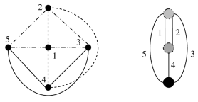
Figure 6: A circuit partition in $K_{5}$, and its touch-graph.

As an example, consider the circuit partition $P$ of $K_{5}$ illustrated in Figure 6. The reader may verify that if $C$ and $D$ are the Euler circuits of $K_{5}$ indicated in Figure 5 then the transitions appearing in $P$ are $\phi_{C}(1)=\psi_{D}(1)$, $\phi_{C}(2)=\psi_{D}(2)$, $\chi_{C}(3)=\chi_{D}(3)$, $\chi_{C}(4)=\phi_{D}(4)$ and $\phi_{C}(5)=\chi_{D}(5)$. Consequently

$$M(C,P)=\begin{pmatrix}1&0&1&1&0\\ 0&1&1&1&0\\ 0&0&0&0&0\\ 0&0&0&0&0\\ 0&0&1&0&1\end{pmatrix}\text{ and }M(D,P)=\begin{pmatrix}1&1&1&0&1\\ 1&1&1&0&1\\ 1&1&0&0&0\\ 1&0&0&1&1\\ 1&1&0&0&0\end{pmatrix}\text{.}$$

It is a simple matter to verify that the nonzero elements of $\ker M(C,P)=\ker M(D,P)$ are the vertex cocycles of $Tch(P)$, i.e., the column vectors obtained by transposing $(1,1,1,0,1)$, $(1,1,0,1,0)$ and $(0,0,1,1,1)$.

The following consequence of Theorem 36 allows us to study the transverse circuits of circle graphs using circuits of 4-regular graphs.

Corollary 38.

Let $\gamma$ be a circuit of a 4-regular graph $F$, which is not an Euler circuit of a connected component. Let $\tau(\gamma)$ denote the set of transitions involved in $\gamma$. Then $\tau(\gamma)$ is a dependent set of $M_{\tau}(F)$.

Proof.

Let $\gamma$ be $v_{1},h_{1},h_{1}^{\prime},v_{2},h_{2},\ldots,h_{\ell}^{\prime},v_{\ell+1}=v_{1}$. Then $V(F)=V_{0}\cup V_{1}\cup V_{2}$, where $V_{k}=\{v\in V(F)\mid$ there are precisely $k$ values of $i\in\{1,\ldots,\ell\}$ with $v_{i}=v\}$. If $V_{1}=\varnothing$ then $\gamma$ includes all four half-edges incident on each of $v_{1},\ldots,v_{\ell}$. Consequently no vertex of $V_{2}$ neighbors any vertex outside $V_{2}$, so $\gamma$ is an Euler circuit of a connected component with vertex-set $V_{2}$. By hypothesis, this is not the case; hence $V_{1}\not=\varnothing$.

Arbitrarily choose transitions at vertices of $V_{0}$, and let $P$ denote the circuit partition that involves these transitions in addition to the elements of $\tau(\gamma)$. Let $C$ be any Euler system for $F$. Then Theorem 36 tells us that the vertex cocycle of $\gamma$ in $Tch(P)$ is an element of $\ker M(C,P)$. This vertex cocycle is $V_{1}$, considered as a set of edges in $Tch(P)$.

As $V_{1}\in\ker M(C,P)$, the columns of $M(C,P)$ corresponding to elements of $V_{1}$ sum to $0$. These columns are the columns of $IAS(\mathcal{I}(C))$ corresponding to transitions of $P$ at vertices of $V_{1}$, so they correspond to a subset of $\tau(\gamma)$. As $V_{1}\not=\varnothing$, it follows that $\tau(\gamma)$ is dependent in $M_{\tau}(F)$. ∎

Theorem 5 of the introduction follows readily. If $\gamma$ is not an Euler circuit of a connected component, then Corollary 38 tells us that $\tau(\gamma)$ contains a transverse circuit of $M_{\tau}(F)$. If $\gamma$ is an Euler circuit of a connected component, then that connected component has a non-Euler circuit $\gamma^{\prime}$; necessarily $\left|\tau(\gamma^{\prime})\right|\leq\left|\tau(\gamma)\right|$, and Corollary 38 tells us that $\tau(\gamma^{\prime})$ contains a transverse circuit of $M_{\tau}(F)$.

Figure 7: An Euler circuit and its interlacement graph.

By the way, it can happen that a transverse circuit of $M_{\tau}(F)$ is strictly smaller than every circuit in $F$. See Figure 7 for an example. $F$ is a simple graph, so it has no circuit of size $<3$. But the interlacement graph of the indicated Euler circuit $C$ has a transverse circuit of size two: if $v$ is the vertex at the top of the figure and $w$ is the vertex pendant on $v$ in $\mathcal{I}(C)$ then the columns of $IAS(\mathcal{I}(C))$ representing $\phi_{C}(v)$ and $\chi_{C}(w)$ are equal, so $\{\phi_{C}(v)$, $\chi_{C}(w)\}$ is a transverse circuit.

Before concluding this section we should explain the connection between isotropic minors of circle graphs (as defined in Definition 2) and detachments of 4-regular graphs. Let $F$ be a 4-regular graph, and suppose $t\in\mathfrak{T}(F)$ is a transition at a vertex $v$. Then the detachment of $F$ along $t$ is the 4-regular graph $F^{\prime}$ obtained from $F$ by removing $v$ and forming two new edges from the four half-edges incident at $v$, pairing together the half-edges according to $t$. If $F$ has a loop at $v$, detachment along $t$ may result in one or two “free edges” that have no incident vertex; any such free edge is simply discarded.

If $t$ is not a loop of $M_{\tau}(F)$, $F$ has an Euler system $C$ with $\phi_{C}(v)=t$. As illustrated in Figure 8, $F^{\prime}$ then inherits an Euler system $C^{\prime}$ directly from $C$. Clearly $\mathcal{I}(C^{\prime})$ is the induced subgraph of $\mathcal{I}(C)$ obtained by removing $v$. Consequently $IAS(\mathcal{I}(C^{\prime}))$ is the matrix obtained from $IAS(\mathcal{I}(C))$ by removing the $v$ row and all three columns corresponding to $v$. As the only nonzero entry of the $\phi_{C}(v)$ column is a 1 in the $v$ row, the effect of these removals is that

$$M[IAS(\mathcal{I}(C^{\prime}))]=(M[IAS(\mathcal{I}(C))]/\phi_{C}(v))-\chi_{C}(v)-\psi_{C}(v)\text{.}$$

That is, $M_{\tau}(F^{\prime})$ is the isotropic minor of $M_{\tau}(F)$ obtained by contracting $t$.

If $t$ is a loop of $M_{\tau}(F)$, then $M_{\tau}(F)$ is the direct sum of $M_{\tau}(F^{\prime})$ and the restriction of $M_{\tau}(F)$ to the vertex triple of $v$. Consequently, $M_{\tau}(F^{\prime})$ is again the isotropic minor of $M_{\tau}(F)$ obtained by contracting $t$.

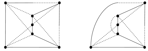
Figure 8: A detachment of a 4-regular graph inherits an Euler circuit.

5 Circle graphs with small transverse circuits

Corollary 38 suggests that in order to characterize circle graphs, we should obtain detailed information about small circuits in small 4-regular graphs.

Proposition 39.

Let $F$ be a 4-regular graph with $<9$ vertices. If $F$ has no circuit of size $\leq 3$, then $F$ is isomorphic to $K_{4,4}$.

Proof.

Suppose $F$ has no circuit of size $<3$; then $F$ is a simple graph. According to data tabulated by Meringer [31], there are only ten simple, 4-regular graphs of order $<9$, up to isomorphism. One is $K_{4,4}$. The other nine are pictured in Figure 9. It is evident that all nine have 3-circuits. ∎

Figure 9: The simple 4-regular graphs of order $\leq 8$, other than $K_{4,4}$.

Close inspection of Figure 9 yields a more elaborate form of Proposition 39, which will also be useful. In stating this proposition we use a convenient shorthand, specifying a circuit by simply listing the incident vertices in order.

Proposition 40.

Let $F$ be a simple 4-regular graph with $<9$ vertices, which is not isomorphic to $K_{4,4}$. Then $F$ has two distinct 3-circuits $\gamma_{1}=v_{1}v_{2}w_{1}$ and $\gamma_{2}=v_{1}v_{2}w_{2}$, and an Euler circuit of the form $v_{1}w_{1}v_{2}v_{1}w_{2}v_{2}$…

Corollary 41.

A simple graph $G$ is a circle graph if and only if $G$ satisfies these two conditions.

1. Every transverse matroid of $G$ is cographic.

2. If an isotropic minor of $G$ of size $\leq 24$ does not have a loop or a pair of intersecting $3$-circuits, then it is isomorphic to $M_{\tau}(K_{4,4})$.

Proof.

Suppose $G$ is an interlacement graph of a 4-regular graph $F$. Condition 1 follows from Corollary 37.

As discussed at the end of Section 4, the isotropic minors of $G$ are isotropic matroids of interlacement graphs of 4-regular graphs obtained from $F$ through detachment. Consequently, if $M$ is an isotropic minor of $G$ of size $\leq 24$ then $M$ is the isotropic matroid of a circle graph $H$ with $\leq 8$ vertices. Proposition 39 tells us that if $H$ is not an interlacement graph of $K_{4,4}$ then it is an interlacement graph of a 4-regular graph with a circuit of size $\leq 3$. Theorem 5 tells us that $H$ has a transverse circuit of size $\leq 3$.

If $M[IAS(H)]$ has a loop, then of course condition 2 is satisfied. Suppose $M[IAS(H)]$ has no loop; then every vertex triple is a 3-circuit. If $H$ has a transverse 2-circuit, then $H$ has two vertices $v$ and $w$ whose vertex triples include elements that are parallel in $M[IAS(H)]$; there is a 3-circuit obtained by replacing one element of the vertex triple of $v$ with a parallel from the vertex triple of $w$. If $H$ has no transverse circuit of size $\leq 2$ then it must have a transverse 3-circuit, which certainly intersects the three corresponding vertex triples.

Suppose conversely that $G$ satisfies both conditions. Condition 1 guarantees that no isotropic minor of $M[IAS(G)]$ is isomorphic to $M[IAS(BW_{3})]$, which has the Fano matroid and the dual Fano matroid as non-cographic transverse matroids. Condition 2 guarantees that no isotropic minor of $G$ is isomorphic to $M[IAS(W_{5})]$ or $M[IAS(W_{7})]$, neither of which is isomorphic to $M_{\tau}(K_{4,4})$ or has a transverse circuit of size $\leq 3$. It follows from Theorem 4 that $G$ is a circle graph. ∎

Conceptually, condition 1 of Corollary 41 may seem to be more interesting than condition 2, because cographic matroids are well-studied and the fact that transverse matroids of circle graphs are cographic is explained by their connection with touch-graphs. However, we have not been able to formulate a matroidal characterization of circle graphs that references only broad properties like “cographic.” Instead, Proposition 40 allows us to replace condition 1 of Corollary 41 with a requirement involving 3-circuits.

Corollary 42.

A simple graph $G$ is a circle graph if and only if every isotropic minor $M$ of $G$, of size $\leq 24$, satisfies at least one of the following conditions:

1. $M$ has a transverse circuit of size $\leq 2$.

2. $M$ has a pair of transverse 3-circuits that are not both contained in any one transversal of $M$.

3. $M$ is isomorphic to $M_{\tau}(K_{4,4})$.

Proof.

Suppose $G$ is an interlacement graph of a 4-regular graph $F$, and $M$ is an isotropic minor of $G$ of size $\leq 24$. Then $M$ is the isotropic matroid of an interlacement graph $H$ of a 4-regular graph $F^{\prime}$ of order $\leq 8$. Suppose $M$ has no loop or transverse 2-circuit, and $H$ is not an interlacement graph of $K_{4,4}$. Then Theorem 5 tells us that $F^{\prime}$ is simple, and Proposition 40 tells us that $F^{\prime}$ has two distinct 3-circuits $\gamma_{1}=v_{1}v_{2}w_{1}$ and $\gamma_{2}=v_{1}v_{2}w_{2}$ that share precisely one edge. Corollary 38 tells us that $\tau(\gamma_{1})$ and $\tau(\gamma_{2})$ are transverse 3-circuits of $M$. As $\gamma_{1}$ and $\gamma_{2}$ do not involve the same transition at $v_{1}$ or $v_{2}$, no subtransversal of $H$ contains more than four elements of $\tau(\gamma_{1})\cup\tau(\gamma_{2})$.

For the converse, suppose $G$ satisfies the statement. Then no isotropic minor of $G$ is isomorphic to $M[IAS(W_{5})]$ or $M[IAS(W_{7})]$, because neither of these isotropic matroids is isomorphic to $M_{\tau}(K_{4,4})$ and neither has any transverse circuit of size $\leq 3$. $BW_{3}$ does have transverse 3-circuits: the neighborhood circuits of the degree-2 vertices are of size 3, and the $\chi_{G}$ elements of the three degree-2 vertices also constitute a transverse circuit. A computer search using the matroid module for Sage [34, 37] verifies that these four are the only transverse 3-circuits of $BW_{3}$, though, and clearly their union is a transversal. ∎

Recall the notation used in the introduction: If $G$ is a simple graph, then $\mathcal{VM}_{8}(G)$ denotes the set of vertex-minors of $G$ with 8 or fewer vertices. Using this notation and the fact that the isotropic minors of $G$ are the isotropic matroids of vertex-minors of $G$, we may rephrase Corollary 42 as follows.

Corollary 43.

A simple graph $G$ is a circle graph if and only if every $H\in\mathcal{VM}_{8}(G)$ that is not an interlacement graph of $K_{4,4}$, is locally equivalent to a graph with a vertex of degree $0$ or $1$ or with two adjacent degree-$2$ vertices.

Proof.

We first prove the if direction. Assume the right-hand side of the equivalence holds. We invoke Corollary 42. Let $M[IAS(H)]$ be an isotropic minor of $G$ of size $\leq 24$. We have $H\in\mathcal{VM}_{8}(G)$. If $H$ is an interlacement graph of $K_{4,4}$, then by Theorem 1 $M[IAS(H)]$ satisfies condition 3 of Corollary 42. If $H$ is locally equivalent to a graph with a vertex of degree $0$ or $1$, then by Theorem 6 $M[IAS(H)]$ satisfies condition 1 of Corollary 42. Finally, if $H$ is locally equivalent to a graph with two adjacent degree-$2$ vertices, then by Theorem 7 $M[IAS(H)]$ satisfies condition 2 of Corollary 42. Thus, by Corollary 42, $G$ is a circle graph.

For the converse, suppose $G$ is a circle graph and $H\in\mathcal{VM}_{8}(G)$ is not an interlacement graph of $K_{4,4}$ and not locally equivalent to a graph with a vertex of degree $0$ or $1$. Then $H$ is isomorphic to an interlacement graph of a 4-regular graph $F$ pictured in Figure 9. As noted in Proposition 40, $F$ has an Euler circuit $C$ of the form $v_{1}w_{1}v_{2}v_{1}w_{2}v_{2}\ldots$. Then $v_{1}$ and $v_{2}$ are adjacent degree-$2$ vertices in $\mathcal{I}(C)$, and $H$ is locally equivalent to a graph isomorphic to $\mathcal{I}(C)$. ∎

6 $K_{4,4}$ vs. $W_{7}$

The results of the preceding section leave us with the task of distinguishing $W_{7}$ from an interlacement graph of $K_{4,4}$. This task is a bit more difficult than one might expect. For instance, it turns out that both $W_{7}$ and an interlacement graph of $K_{4,4}$ have 42 transverse 4-circuits, 168 transverse 6-circuits and no other transverse circuit of size $\leq 7$. Nevertheless, there are several ways to verify that $W_{7}$ is not an interlacement graph of $K_{4,4}$. We mention four in this section, and several more in the next section.

6.1 A distinctive transverse matroid of $W_{7}$

Notice that the transverse matroid $\{\phi_{1}$, $\phi_{2}$, $\chi_{3}$, $\phi_{4}$, $\phi_{5}$, $\psi_{6}$, $\psi_{7}$, $\phi_{8}\}$ of $W_{7}$ contains only two circuits, $\{\phi_{1}$, $\phi_{2}$, $\chi_{3}$, $\phi_{4}\}$ and $\{\phi_{5}$, $\psi_{6}$, $\psi_{7}$, $\phi_{8}\}$. (Here vertex 1 is the central vertex of the wheel, and the outer vertices are numbered consecutively around the rim.) In contrast, it turns out that no transverse matroid of an interlacement graph of $K_{4,4}$ contains precisely two circuits. As a first step in verifying this assertion, note that if a matroid has precisely two circuits then the circuit elimination property guarantees that the two circuits must be disjoint.

Theorem 44.

The smallest transverse circuits of $M_{\tau}(K_{4,4})$ are of size 4, and there is no non-transverse 4-circuit. If a transverse matroid $M$ of $M_{\tau}(K_{4,4})$ contains two disjoint circuits then they are of size 4, and $M$ contains six transverse circuits of size 4.

Proof.

Let $V(K_{4,4})=\{1,2,3,4,a,b,c,d\}$, and consider the Euler circuit $C$ given by the double occurrence word $a1b2c3b4a3d4c1d2$. If $I$ is the $V(\mathcal{I}(C))\times V(\mathcal{I}(C))$ identity matrix then $IAS(\mathcal{I}(C))$ is the $V(\mathcal{I}(C))\times W(\mathcal{I}(C))$ matrix

$$\noindent\setcounter{MaxMatrixCols}{18}\begin{pmatrix}&&0&1&0&0&1&0&0&1&1&1&0&0&1&0&0&1\\ &&1&0&0&0&1&1&0&0&1&1&0&0&1&1&0&0\\ &&0&0&0&1&1&1&0&0&0&0&1&1&1&1&0&0\\ &&0&0&1&0&1&0&0&1&0&0&1&1&1&0&0&1\\ I&&1&1&1&1&0&0&1&0&1&1&1&1&1&0&1&0\\ &&0&1&1&0&0&0&1&0&0&1&1&0&0&1&1&0\\ &&0&0&0&0&1&1&0&1&0&0&0&0&1&1&1&1\\ &&1&0&0&1&0&0&1&0&1&0&0&1&0&0&1&1\end{pmatrix}\text{.}$$

The rows are indexed in $1,2,3,4,a,b,c,d$ order, as are the columns in each part of $\begin{pmatrix}I&\mathcal{I}(C)&I+\mathcal{I}(C)\end{pmatrix}$.

Computer programs and visual inspection indicate that no single column is identically 0, no two columns sum to 0, and every set of three columns that sum to 0 corresponds to a vertex triple. The circuits of size 4 are all transverse circuits, and there are 42 of them. These circuits fall into two sets:

• For each of the six 2-element subsets $\{i,j\}$ of $\{1,2,3,4\}$ and each of the six 2-element subsets $\{x,y\}$ of $\{a,b,c,d\}$, there is a transverse circuit that includes the transitions determined by the single transitions $ixj$, $xjy$, $jyi$ and $yix$. For instance, $\{\phi_{C}(1)$, $\phi_{C}(a)$, $\chi_{C}(2)$, $\phi_{C}(b)\}$ and $\{\chi_{C}(3)$, $\chi_{C}(c)$, $\phi_{C}(4)$, $\phi_{C}(d)\}$ are transverse circuits of this type.

• For each of the six 2-element subsets $\{i,j\}$ of $\{1,2,3,4\}$, there is a transverse circuit that includes the transitions determined by the single transitions $iaj$, $ibj$, $icj$ and $idj$. Notice that $\{i,j\}$ and its complement in $\{1,2,3,4\}$ determine the same four transitions, so there are only three transverse circuits of this type. Similarly, there are three transverse circuits corresponding to 2-element subsets of $\{a,b,c,d\}$. For instance, $\{i,j\}=\{1,2\}$ and $\{3,4\}$ both yield $\{\phi_{C}(a)$, $\phi_{C}(b)$, $\chi_{C}(c)$, $\phi_{C}(d)\}$ and $\{x,y\}=\{a,b\}$ and $\{c,d\}$ both yield $\{\phi_{C}(1)$, $\chi_{C}(2)$, $\chi_{C}(3)$, $\phi_{C}(4)\}$.

Figure 10: The cocycle matroid of this graph is isomorphic to a transverse matroid of $W_{7}$, but not of $M_{\tau}(K_{4,4})$.

Now, suppose a transverse matroid $M$ of $M_{\tau}(K_{4,4})$ contains two disjoint circuits. As $M$ has 8 elements and $M_{\tau}(K_{4,4})$ has no transverse circuit of size $<4$, the two circuits must both be of size 4. If the two disjoint circuits are of the first type, then after re-indexing we may suppose they arise from the circuits $1a2b$ and $3c4d$. Then $M$ also contains transverse circuits of the first type corresponding to the circuits $1c2d$ and $3a4b$. Moreover, $M$ contains the transverse circuits of the second type corresponding to $\{1,2\}$ (or $\{3,4\}$) and $\{a,b\}$ (or $\{c,d\}$). If the two disjoint transverse circuits are of the second type, we may presume one corresponds to $\{1,2\}$ (or $\{3,4\}$) and the other to $\{a,b\}$ (or $\{c,d\}$). Then $M$ contains the transverse circuits of the first type that correspond to the circuits $1a2b$, $3c4d$, $1c2d$ and $3a4b$. Finally, it is impossible for the two disjoint circuits to include one of the first type and one of the second type. ∎

Corollary 45.

Every interlacement graph of an Euler circuit of $K_{4,4}$ is of diameter $\leq 2$.

Proof.

According to Theorem 8, a graph of diameter $>2$ has a subtransversal that contains two disjoint circuits, whose union contains no other circuit. Theorem 44 tells us that $M_{\tau}(K_{4,4})$ has no such subtransversal. ∎

6.2 Interlacement graphs of $K_{4,4}$ are not 3-regular

We call a simple graph strictly supercubic if all the vertices are of degree $\geq 3$, and there is at least one vertex of degree $>3$.

Proposition 46.

Every interlacement graph of an Euler circuit of $K_{4,4}$ is strictly supercubic.

Proof.

Let $G$ be an interlacement graph of $K_{4,4}$; then $M[IAS(G)]\cong M_{\tau}(K_{4,4})$, so Theorem 44 tells us that the smallest transverse circuits in $M[IAS(G)]$ are of size 4. By Theorem 6, this implies that all the vertices of $G$ are of degree $\geq 3$. If any vertex is of degree $>3$ we are done, so we may suppose $G$ is 3-regular.

If $G$ is not connected it has two components, each isomorphic to $K_{4}$. But then if $v$ and $w$ are adjacent vertices of $G$, $\{\psi_{G}(v),\psi_{G}(w)\}$ is a transverse 2-circuit of $M[IAS(G)]$, contradicting Theorem 44. We conclude that $G$ is connected.

Let $v_{1}$ and $v_{2}$ be nonadjacent vertices of $G$. If they share all their neighbors, then $\{\chi_{G}(v_{1}),\chi_{G}(v_{2})\}$ is a transverse 2-circuit of $M[IAS(G)]$. Theorem 44 tells us that this is impossible. On the other hand, if they share no neighbor then the diameter of $G$ is $>2$. Corollary 45 tells us that this is impossible.

Figure 11: The connected, cubic simple graphs of order 8.

According to Meringer [31], there are five connected, simple 3-regular graphs with 8 vertices. They are displayed in Figure 11. We observe that the first of these graphs has a pair of nonadjacent vertices that share all their neighbors, and each of the next three has a pair of nonadjacent vertices that share no neighbor. It is not immediately apparent, but the fifth graph pictured in Figure 11 is locally equivalent to the fourth (up to isomorphism); see Figure 12 for details. (It is easy to see that the last graph in Figure 12 is isomorphic to the fourth graph in Figure 11, if you first observe that each has precisely two 3-circuits.) ∎

Figure 12: A local equivalence.

By the way, there is a considerably longer proof of Proposition 46 that may be of interest in spite of its length. Theorems 6 and 44 tell us that if $G$ is an interlacement graph of $K_{4,4}$ then all the transverse circuits of $G$ are of size $\geq 4$, and all the vertices of $G$ are of degree $\geq 3$. Consequently, $G$ is either cubic or strictly supercubic. According to [42], though, every 3-regular circle graph has transverse circuits of size $2$; hence $G$ is not 3-regular.

Corollary 47.

Every interlacement graph of an Euler circuit of $K_{4,4}$ has a vertex of degree 5.

Proof.

As observed at the beginning of this section, a computer search (again using the matroid module for Sage [34, 37]) indicates that the transverse circuits of $M_{\tau}(K_{4,4})$ of size $<9$ are all of size 4, 6 or 8. Consequently Theorem 6 guarantees that if $G$ is an interlacement graph of an Euler circuit of $K_{4,4}$ then the vertex-degrees in $G$ are elements of the set $\{3,5,7\}$. Proposition 46 assures us that $G$ must have at least one vertex of degree 5 or 7.

Suppose $G$ has no vertex of degree 5. If $v_{1}$ and $v_{2}$ both have degree $7$ then the $\psi_{G}(v_{1})$ and $\psi_{G}(v_{2})$ columns of $IAS(G)$ are the same, so $\{\psi_{G}(v_{1}),\psi_{G}(v_{2})\}$ is a transverse 2-circuit of $G$. But $M_{\tau}(K_{4,4})$ has no transverse 2-circuit, so this cannot be the case. That is, $G$ must have one vertex $v_{1}$ of degree 7, and seven vertices of degree $3$. The induced subgraph $G-v_{1}$ is then $2$-regular. As $G$ is simple, there are only two possibilities: $G-v_{1}$ is either a 7-circuit or the disjoint union of a 3-circuit and a 4-circuit. The former is impossible, as $v_{1}$ would neighbor all the vertices on the 7-circuit and consequently $G$ would be isomorphic to $W_{7}$. The latter is also impossible: two nonadjacent vertices $v$ and $w$ on the 4-cycle would have identical open neighborhoods in $G$, as $v$ and $w$ would have the same neighbors on the 4-cycle and $v$ and $w$ would also be adjacent to $v_{1}$; consequently $\{\chi_{G}(v),\chi_{G}(w)\}$ would be a transverse 2-circuit in $M[IAS(G)]$.

We conclude that $G$ must have a vertex of degree 5. ∎

6.3 A distinctive transverse matroid of $M_{\tau}(K_{4\text{,}4})$

Here is another way to distinguish $W_{7}$ from an interlacement graph of $K_{4,4}$.

Proposition 48.

Let $P$ be a 4-element circuit partition of $K_{4,4}$. Then either $Tch(P)$ is obtained from a 4-cycle by doubling all edges, or $Tch(P)$ is obtained from a complete graph by doubling two non-incident edges. In contrast, the nullity-3 transverse matroids of $W_{7}$ are all isomorphic to the cocycle matroid of a complete graph with two non-incident edges doubled.

Proof.

The proposition has been verified with computer programs (again using Sage [34, 37]). ∎

Figure 13: The cocycle matroid of this graph is isomorphic to a transverse matroid of $M_{\tau}(K_{4,4})$, but not of $W_{7}$.

7 Circle graph characterizations

As discussed in the introduction, we deduce circle graph characterizations from Bouchet’s theorem and the observations of Sections 5 and 6 by combining conditions that exclude $W_{5}$, $BW_{3}$ and $W_{7}$ as vertex-minors, and do not exclude any circle graph. For instance, Corollary 41 and Theorem 44 yield Theorem 10 in this way, and Corollaries 43 and 47 yield Theorem 12. Other characterizations are obtained using different combinations of the properties listed below. Properties not mentioned earlier in the paper have been verified using Sage [34, 37].

Properties of $W_{5}$: It is locally equivalent to a cubic graph, it has no transverse circuit of size $\leq 3$, and it is not locally equivalent to any graph with a vertex of degree $\leq 2$.

Properties of $BW_{3}$: It has some non-cographic transverse matroids, and it is not locally equivalent to a graph with either a vertex of degree $\leq 1$ or adjacent vertices of degree 2.

Properties of $W_{7}$: It is locally equivalent to a 3-regular graph of diameter 3, it is not locally equivalent to any graph with a vertex of degree $\leq 2$, it has no transverse circuit of size $\leq 3$, it has the cocycle matroid of the graph of Figure 10 as a transverse matroid, it does not have the cocycle matroid of the graph of Figure 13 as a transverse matroid, it has 42 transverse matroids of nullity 3, and its isotropic matroid has 336 automorphisms.

Properties of a circle graph of order $\leq 8$ not associated with $K_{4,4}$: It has transverse circuits of size $\leq 3$, it has cographic transverse matroids, and it is locally equivalent to a graph with a vertex of degree $\leq 1$ or a pair of adjacent degree-2 vertices.

Properties of a circle graph associated with $K_{4,4}$: It has cographic transverse matroids, it has a vertex of degree 5, its diameter is $\leq 2$, it does not have the cocycle matroid of the graph of Figure 10 as a transverse matroid, it does not have a transverse matroid with two disjoint circuits and no other circuit, it has the cocycle matroid of the graph of Figure 13 as a transverse matroid, it has 45 transverse matroids of nullity 3, and its isotropic matroid has 1152 automorphisms.

8 Bipartite circle graphs

In this section we discuss Theorem 11 of the introduction, and several associated results. These results differ from the characterizations of general circle graphs discussed above in that they do not rely on Bouchet’s theorem. Their foundation is an earlier result of de Fraysseix [24]; a proof is included for the reader’s convenience.

Proposition 49.

([24, Proposition 6]) Let $G$ be a bipartite simple graph, with vertex classes $V_{1}$ and $V_{2}$. Then $G$ is a circle graph if and only if the transverse matroid $\phi_{G}(V_{1})\cup\chi_{G}(V_{2})$ is a planar matroid.

Proof.

Let the adjacency matrix of $G$ be

$$A=\begin{pmatrix}0&A_{12}\\ A_{21}&0\end{pmatrix}.$$

Then the transverse matroids $M_{1}=\phi_{G}(V_{1})\cup\chi_{G}(V_{2})$ and $M_{2}=\chi_{G}(V_{1})\cup\phi_{G}(V_{2})$ are represented by $\begin{pmatrix}I_{1}&A_{12}\end{pmatrix}$ and $\begin{pmatrix}A_{21}&I_{2}\end{pmatrix}$, where $I_{1}$ and $I_{2}$ are identity matrices. As $A_{12}$ and $A_{21}$ are transposes of each other, $M_{1}$ and $M_{2}$ are dual matroids.

If $G$ is a circle graph then Corollary 37 tells us that $M_{1}$ and $M_{2}$ are both cographic. They are each other’s duals, so they must be planar.

Suppose conversely that $M_{1}$ is a planar matroid; then $M_{2}$ is planar too. Let $H$ be a plane graph whose cycle matroid is $M_{1}$. We presume that $H$ is connected, its dual $H^{\ast}$ is connected, and $H$ and $H^{\ast}$ may be drawn together in the plane in such a way that all their edges are smooth curves, in general position. We identify $E(H)$ and $E(H^{\ast})$ with $V(G)$.

$H$ has a spanning tree $T$ corresponding to the basis $\phi_{G}(V_{1})$ of $M_{1}$. Choose an $\varepsilon$-neighborhood $D$ of $T$; $D$ is homeomorphic to a disk, so its boundary $\partial D$ is homeomorphic to a circle. As long as $\varepsilon$ is sufficiently small, each element $e\in E(H)-E(T)$ intersects $D$ in two short arcs. Use $e$ to label the end-points of these arcs on $\partial D$. Also choose two points of $\partial D$ for each edge of $T$, one on each side of the midpoint; label these two points with that edge. If we trace the circle $\partial D$ and read off the labeled points in order then we obtain a double occurrence word $W$, in which each edge of $H$ appears twice.

Consider an edge $e\in E(T)$, and write $W$ as $eW_{1}eW_{2}$. Let $\gamma$ be a simple closed curve obtained by following $\partial D$ from one point labeled $e$ to the other point labeled $e$, and then crossing through $D$ back to the first point labeled $e$. Clearly then $\gamma$ encloses one connected component of $T-e$. If $e^{\prime}$ is an edge of the connected component of $T-e$ enclosed by $\gamma$, then both points of $\partial D$ labeled $e^{\prime}$ appear on $\gamma$. If $e^{\prime}$ is an edge of the connected component of $T-e$ not enclosed by $\gamma$, then neither point of $\partial D$ labeled $e^{\prime}$ appears on $\gamma$. Either way, we see that $e$ and $e^{\prime}$ are not interlaced with respect to $W$.

Now consider an edge $e\in E(H)-E(T)$, and write $W$ as $eW_{1}eW_{2}$. Suppose $e^{\prime}\neq e\in E(H)-E(T)$. If $e^{\prime}$ appears precisely once in $W_{1}$, then it is not possible to draw $e$ and $e^{\prime}$ without a crossing outside $D$; as there is no such crossing, it cannot be that $e^{\prime}$ appears precisely once in $W_{1}$. That is, $e$ and $e^{\prime}$ are not interlaced with respect to $W$. Considering the preceding paragraph, we deduce that the interlacement graph $\mathcal{I}(W)$ is bipartite, with $E(T)$ and $E(H)-E(T)$ as vertex-classes.

Again, let $e\in E(H)-E(T)$, and write $W$ as $eW_{1}eW_{2}$. Remove all appearances of edges not in $T$ from $W_{1}$ and $W_{2}$; the result is two walks in $T$ connecting the end-vertices of $e$. If we remove the edges that appear twice in either of these walks, we must obtain the unique path in $T$ connecting the end-vertices of $e$. We conclude that the fundamental circuit of $e$ with respect to $T$ in $H$ coincides with the closed neighborhood of $e$ in $\mathcal{I}(W)$. As $T$ is a spanning tree of $H$ corresponding to the basis $\phi_{G}(V_{1})$ of $M_{1}$, the fundamental circuit of $e$ with respect to $T$ in $H$ is the same as the closed neighborhood of $e$ in $G$.

As $G$ and $\mathcal{I}(W)$ are both bipartite simple graphs with a vertex-class corresponding to $V_{1}=E(T)$, it follows that $G=\mathcal{I}(W)$. ∎

Note that in the situation of Proposition 49, $G$ is a special kind of circle graph: it is an interlacement graph of a planar 4-regular graph $F$. To construct such an $F$, start with the closed curve $\partial D$ mentioned in the proof of Proposition 49. $F$ has a vertex at the midpoint of each edge of $T$, and a vertex outside $D$ on each edge of $E(H)-E(T)$; edges are inserted so that the word $W$ corresponds to an Euler circuit of $F$. It is a simple matter to draw $F$ in the plane using the closed curve $\partial D$ as a guide.

Proposition 49 implies the following.

Theorem 50.

Let $G$ be a simple graph. Then each of these conditions implies the others.

1. $G$ is the interlacement graph of an Euler system of a planar 4-regular graph.

2. There are disjoint transversals $T_{1},T_{2}$ of $W(G)$ such that $r(T_{1})+r(T_{2})=\left|V(G)\right|$ and

   $$M[IAS(G)]\mid(T_{1}\cup T_{2})$$

   is a planar matroid.

3. $G$ is locally equivalent to a bipartite graph, and all the transverse matroids of $G$ are cographic.

Proof.

If $G$ is a circle graph associated with a planar 4-regular graph then it is well known that $G$ is locally equivalent to a bipartite circle graph; see [35] for instance. This and Corollary 37 give us the implication $1\Rightarrow 3$.

Suppose condition 3 holds, and let $H$ be a bipartite graph locally equivalent to $G$. As there is an induced isomorphism between the isotropic matroids of $G$ and $H$, we may verify condition 2 for $G$ by verifying it for $H$. Let $V(H)=V_{1}\cup V_{2}$ with $V_{1}$ and $V_{2}$ both stable sets of $H$. Then the adjacency matrix of $H$ is

$$A=\begin{pmatrix}0&A_{12}\\ A_{21}&0\end{pmatrix}.$$

Consider the transversals $T_{1}=\phi_{H}(V_{1})\cup\chi_{H}(V_{2})$ and $T_{2}=\phi_{H}(V_{2})\cup\chi_{H}(V_{1})$. Notice that $r(T_{i})=\left|V_{i}\right|$ for each $i$, so $r(T_{1})+r(T_{2})=\left|V(G)\right|$. Moreover, the transverse matroids $M[IAS(H)]\mid T_{1}$ and $M[IAS(H)]\mid T_{2}$ are represented by $\begin{pmatrix}I_{1}&A_{12}\end{pmatrix}$ and $\begin{pmatrix}A_{21}&I_{2}\end{pmatrix}$, where $I_{1}$ and $I_{2}$ are identity matrices. As $A_{12}$ and $A_{21}$ are transposes, these two matroids are duals. Both are cographic by condition 3, so both are planar. Notice that

$$\begin{pmatrix}I&A\end{pmatrix}=\begin{pmatrix}I_{1}&0&0&A_{12}\\ 0&I_{2}&A_{21}&0\end{pmatrix},$$

and consequently

$$M[IAS(H)]\mid(T_{1}\cup T_{2})=(M[IAS(H)]\mid T_{1})\oplus(M[IAS(H)]\mid T_{2})$$

is a direct sum of planar matroids. It follows that $M[IAS(H)]\mid(T_{1}\cup T_{2})$ is a planar matroid.

Suppose now that condition 2 holds, and $G$ has transversals $T_{1}$,  $T_{2}$ as described. Let $B_{1}$ be a basis of $M[IAS(G)]\mid T_{1}$, let $V_{1}=\{v\in v(G)\mid B_{1}$ contains an element of the vertex triple of $v\}$, and let $V_{2}=V(G)-V_{1}$. Let $B_{2}\subseteq T_{2}$ consist of the elements of $T_{2}$ corresponding to elements of $V_{2}$. As discussed in [19, Section 4], $B=B_{1}\cup B_{2}$ is a basis of $M[IAS(G)]$ and there is a graph $H$ that is locally equivalent to $G$, such that (a) an induced isomorphism $\beta:M[IAS(G)]\rightarrow M[IAS(H)]$ maps $B$ to $\{\phi_{H}(v)\mid v\in V(H)\}$ and (b) $H$ is bipartite with vertex-classes $\beta(V_{1})$ and $\beta(V_{2})$. It follows from (b) that for $i\neq j\in\{1,2\}$ the induced isomorphism maps $T_{i}$ to $\phi_{H}(V_{i})\cup\chi_{H}(V_{j})$. Proposition 49 and the subsequent discussion imply that condition 1 holds. ∎

It is important to realize that although $BW_{3}$ is the only one of Bouchet’s circle graph obstructions with non-cographic transverse matroids, condition 3 of Theorem 50 does not imply that a bipartite non-circle graph must have $BW_{3}$ as a vertex-minor. For instance, a computer search using Sage [34, 37] indicates that $BW_{3}$ is not a vertex-minor of the bipartite graph $BW_{4}$ pictured on the left in Figure 14. Nevertheless $BW_{4}$ is not a circle graph. One way to verify this assertion is to observe that the transverse matroid $\{\chi_{1}$, $\phi_{2}$, $\chi_{3}$, $\phi_{4}$, $\chi_{5}$, $\phi_{6}$, $\chi_{7}$, $\phi_{8}$, $\phi_{9}\}$ is not cographic. Indeed, this transverse matroid is isomorphic to the cycle matroid $M(K_{3,3})$; an isomorphism is indicated by the labels $1,2,\ldots,9$ in the figure. (Notice that the labels denote vertices of $BW_{4}$ and edges of $K_{3,3}$.) Another way to verify that $BW_{4}$ is not a circle graph is to obtain $W_{5}$ as a vertex-minor; this can be done by performing local complementations with respect to vertices 2, 4 and 7, and then removing them.

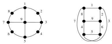
Figure 14: $BW_{4}$ and $K_{3,3}$.

Observe that the implication $3\Rightarrow 1$ of Theorem 50 tells us that the converse of Corollary 37 holds for graphs that are locally equivalent to bipartite graphs. This observation yields the equivalence between the first two properties mentioned in Theorem 11 of the introduction. The next result implies that the third property mentioned in Theorem 11 is equivalent to the the first two.

Corollary 51.

Let $G$ be a bipartite simple graph. Then $G$ is a circle graph if and only if neither $BW_{3}$ nor $BW_{4}$ is a vertex-minor.

Proof.

Of course, if $BW_{3}$ or $BW_{4}$ is a vertex-minor then $G$ is not a circle graph.

For the converse, suppose $G$ is not a circle graph. If $V_{1}$ and $V_{2}$ are the vertex-classes of $G$ then Proposition 49 tells us that the transverse matroid $M=\phi_{G}(V_{1})\cup\chi_{G}(V_{2})$ is not a planar matroid. As noted in the proof of Proposition 49, the transverse matroid $M^{\ast}=\phi_{G}(V_{2})\cup\chi_{G}(V_{1})$ is the dual of $M$; so of course $M^{\ast}$ is not planar either.

Suppose for the moment that $M$ is minor-minimal with regard to nonplanarity. Then $M$ or $M^{\ast}$ is isomorphic to one of $F_{7}$, $M(K_{3,3})$, $M(K_{5})$, so $G$ is a fundamental graph of one of these matroids. The fundamental graphs of a binary matroid are all equivalent under edge pivots, so they are certainly locally equivalent; hence it suffices to verify that one fundamental graph of each of $F_{7}$, $M(K_{3,3})$, and $M(K_{5})$ has $BW_{3}$ or $BW_{4}$ as a vertex-minor. $BW_{3}$ is a fundamental graph of $F_{7}$, and $BW_{4}$ is a fundamental graph of $M(K_{3,3})$.  For $K_{5}$, consider the fundamental graph pictured on the left in Figure 15. (The labels indicate an isomorphism between the transverse matroid $\{\phi_{1}$, $\chi_{2}$, $\chi_{3}$, $\chi_{4}$, $\chi_{5}$, $\chi_{6}$, $\chi_{7}$, $\phi_{8}$, $\phi_{9}$, $\phi_{10}\}$ and $M(K_{5})$.) Clearly $BW_{3}$ is a vertex-minor, obtained by first performing local complementations at the vertices $2$, $3$, $4$, and then removing them.

Proceeding inductively, suppose that $M$ is not minor-minimal with regard to nonplanarity. Then there is an $m\in M$ such that $M/m$ or $M-m$ is also nonplanar. If $M-m$ is nonplanar, then $M^{\ast}/m=(M-m)^{\ast}$ is nonplanar. Consequently by interchanging $V_{1}$ and $V_{2}$ if necessary, we may presume that $M/m$ is nonplanar.

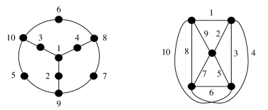
Figure 15: A fundamental graph of $K_{5}$.

If $m=\phi_{G}(v)\in\phi_{G}(V_{1})$ then $M/m$ is a transverse matroid of $G-v\,$, so applying the inductive hypothesis to $G-v$ implies that $BW_{3}$ or $BW_{4}$ is a vertex-minor of $G$. If $m=\chi_{G}(v)\in\chi_{G}(V_{2})$ is a loop of $M$, then $v$ is an isolated vertex of $G$, and again we may apply the inductive hypothesis to $G-v$. If $m=\chi_{G}(v)\in\chi_{G}(V_{2})$ is not a loop of $M$, then $v$ has a neighbor $w\in V_{1}$. In this case the edge pivot $G^{vw}$ is a bipartite graph with vertex classes $V_{1}\Delta\{v,w\}$ and $V_{2}\Delta\{v,w\}$, and an induced isomorphism $\beta:M[IAS(G)]\rightarrow M[IAS(G^{vw})]$ has $\beta(\phi_{G}(w))=\chi_{G^{vw}}(w)$ and $\beta(\chi_{G}(v))=\phi_{G^{vw}}(v)$ [40]. As $\beta(M)$ is isomorphic to $M$, it too is nonplanar; and so is $\beta(M)/\phi_{G^{vw}}(v)\cong M/\chi_{G^{vw}}(v)$. As $\beta(M)/\phi_{G^{vw}}(v)$ is a transverse matroid of $G^{vw}-v$, the inductive hypothesis implies that $BW_{3}$ or $BW_{4}$ is a vertex-minor of $G^{vw}$, and hence of $G$. ∎

9 Crossing numbers of 4-regular graphs

A simple construction indicates that every 4-regular graph can be obtained from a planar 4-regular graph through detachment. Examples appear in Figure 9: the graphs in the top corner positions are detachments of the planar graphs directly below them.

Theorem 52.

Every 4-regular graph is a detachment of a planar 4-regular graph.

Proof.

Draw a 4-regular graph $F$ in the plane, with its edges in general position. That is, the only failures of planarity are points where two edges cross. To obtain a planar graph with $F$ as a detachment, replace each edge-crossing with a vertex. ∎

This leads to yet another characterization of circle graphs:

Corollary 53.

A graph is a circle graph if and only if it is a vertex-minor of a bipartite circle graph.

Proof.

If $G$ is a vertex-minor of any circle graph (bipartite or not), then $G$ itself is a circle graph. For the converse, suppose $G$ is a circle graph associated with a 4-regular graph $F$. According to Theorem 52, $F$ is a detachment of a plane 4-regular graph $\hat{F}$; then $G$ is a vertex-minor of every circle graph associated with $\hat{F}$, as discussed at the end of Section 4. Theorem 50 tells us that some circle graph associated with $\hat{F}$ is bipartite. ∎

Consequently, a simple graph is a circle graph if and only if it is a vertex-minor of some graph that satisfies Theorem 50. Considering condition 2 of Theorem 50, one might hope that Corollary 53 would lead to a characterization of circle graphs using some matroidal property of the unions of pairs of transversals. We do not know what such a property might be, though.

We close with some comments about the connection between pairs of transverse matroids of circle graphs and a well-known measure of non-planarity, the crossing number.

Proposition 54.

Let $G$ be a simple graph. If $G$ is the interlacement graph of an Euler system of a 4-regular graph of crossing number $k$, then there are disjoint transversals $T_{1},T_{2}$ of $W(G)$ such that $r(T_{1})+r(T_{2})\leq\left|V(G)\right|+k$.

Proof.

If $k=0$, the result follows from Theorem 50. Proceeding inductively, suppose $k\geq 1$ and $F$ is a 4-regular graph of crossing number $k$ with $G$ as interlacement graph. Let $F^{\prime}$ be the graph obtained by replacing one crossing with a vertex $v$. Then by the inductive hypothesis $M_{\tau}(F^{\prime})$ has disjoint transversals $T_{1}^{\prime},T_{2}^{\prime}$ such that $r(T_{1}^{\prime})+r(T_{2}^{\prime})\leq\left|V(G)\right|+1+k-1$. As $M[IAS(G)]=M_{\tau}(F)$ is an isotropic minor of $M_{\tau}(F^{\prime})$ obtained by removing the vertex triple of $v$, $T_{1}^{\prime}$ and $T_{2}^{\prime}$ yield disjoint transversals $T_{1},T_{2}$ of $W(G)$. Contraction and deletion cannot raise ranks, so $r(T_{1})\leq r(T_{1}^{\prime})$ and $r(T_{2})\leq r(T_{2}^{\prime})$. ∎

Proposition 54 detects the crossing numbers of some 4-regular graphs. For instance, consider the 4-regular graph $F$ pictured in the lower left-hand corner of Figure 9. Observe that $F$ has precisely four 3-circuits, in two pairs each of which has a shared edge. No circuit partition can include two 3-circuits that share an edge, so a circuit partition of $F$ includes at most two 3-circuits. As $F$ has 16 edges, it follows that every circuit partition includes $\leq 4$ circuits. Theorem 36 then tells us that every transversal of $M_{\tau}(F)$ is of rank $\geq 5$, so the smallest possible value of $r(T_{1})+r(T_{2})$ is 10. According to Proposition 54, this fact guarantees that the crossing number of $F$ is $\geq 2$; as the drawing in Figure 9 has two crossings, we conclude that the crossing number of $F$ is 2.

Proposition 54 is not always so precise. For instance, the reader will have little trouble finding a pair of 4-element circuit partitions in $K_{4,4}$ that do not share any transition. The corresponding transversals of $M_{\tau}(K_{4,4})$ are of rank 5, so they satisfy Proposition 54 with $k=2$. But it is well known that the crossing number of $K_{4,4}$ is 4, not 2.

Let $F$ now denote the 7-vertex 4-regular graph pictured in the middle of the top row of Figure 9. The figure suggests that the crossing number of $F$ is 2, and it is not very hard to show that this is indeed the case. However Figure 16 indicates two partitions of $E(F)$ into four circuits. According to Theorem 36 both of the corresponding transversals of $M_{\tau}(F)$ have rank 4, so they satisfy the necessary condition of Proposition 54 with $k=1$. They do not satisfy the stronger necessary condition of Proposition 55, though.

Figure 16: Two circuit partitions in a graph of crossing number 2.

Proposition 55.

Suppose $G$ is the interlacement graph of an Euler system of a 4-regular graph of crossing number $1$, but is not the interlacement graph of an Euler system of any planar 4-regular graph. Then there are disjoint transversals $T_{1},T_{2}$ of $W(G)$ such that $r(T_{1})+r(T_{2})=\left|V(G)\right|+1$ and $M[IAS(G)]\mid(T_{1}\cup T_{2})$ is a planar matroid.

Proof.

Suppose $F$ is a 4-regular graph with an Euler system $C$ such that $\mathcal{I}(C)=G$, and $F$ has crossing number 1. Let $F^{\prime}$ be a planar 4-regular graph with a vertex $v$ such that detachment at $v$ yields $F$. Let $\tau_{0}(v)$ be the transition that is detached. It is not part of the boundary circuit of a face of $F^{\prime}$; if it were, the detachment would be planar. $M_{\tau}(F^{\prime})$ has transversals $T_{1}^{\prime},T_{2}^{\prime}$ as in Theorem 50, and $\tau_{0}(v)$ is not included in either $T_{1}^{\prime}$ or $T_{2}^{\prime}$; let $\tau_{1}(v)\in T_{1}^{\prime}$ and $\tau_{2}(v)\in T_{2}^{\prime}$ be the other two transitions at $v$. Then $M_{\tau}(F)=(M_{\tau}(F^{\prime})/\tau_{0}(v))-\tau_{1}(v)-\tau_{2}(v)$.

Let $S=T_{1}^{\prime}\cup T_{2}^{\prime}\cup\{\tau_{0}(v)\}$, and recall that

$$M_{\tau}(F^{\prime})\mid(T_{1}^{\prime}\cup T_{2}^{\prime})=(M_{\tau}(F^{\prime})\mid T_{1}^{\prime})\oplus(M_{\tau}(F^{\prime})\mid T_{2}^{\prime}).$$

Then the matroid $M=M_{\tau}(F^{\prime})\mid S$ has five kinds of circuits: (i) Each circuit of $M_{\tau}(F^{\prime})\mid T_{1}^{\prime}$ or $M_{\tau}(F^{\prime})\mid T_{2}^{\prime}$ is also a circuit of $M$. (ii) The vertex triple $\{\tau_{0}(v)$, $\tau_{1}(v)$, $\tau_{2}(v)\}$ is a circuit of $M$. (iii) For each circuit $\gamma_{1}$ of $M_{\tau}(F^{\prime})\mid T_{1}^{\prime}$ that contains $\tau_{1}(v)$, $M$ also has the circuit $(\gamma_{1}-\{\tau_{1}(v)\})\cup\{\tau_{0}(v)$, $\tau_{2}(v)\}$. (iv) For each circuit $\gamma_{2}$ of $M_{\tau}(F^{\prime})\mid T_{1}^{\prime}$ that contains $\tau_{2}(v)$, $M$ also has the circuit $(\gamma_{2}-\{\tau_{2}(v)\})\cup\{\tau_{0}(v)$, $\tau_{1}(v)\}$. (v) For each pair of circuits $\gamma_{1}$, $\gamma_{2}$ as in (iii) and (iv), $M$ has the circuit $(\gamma_{1}-\{\tau_{1}(v)\})\cup(\gamma_{2}-\{\tau_{2}(v)\})\cup\{\tau_{0}(v)\}$.

Let $T_{1},T_{2}$ be the transversals in $M_{\tau}(F)$ that correspond to $T_{1}^{\prime}$ and $T_{2}^{\prime}$. Then $r(T_{1})+r(T_{2})\leq r(T_{1}^{\prime})+r(T_{2}^{\prime})=\left|V(F^{\prime})\right|=\left|V(F)\right|+1$. Also,

$$M_{\tau}(F)\mid(T_{1}\cup T_{2})=(M-\tau_{1}(v)-\tau_{2}(v))/\tau_{0}(v)$$

has only two kinds of circuits: (i) Each circuit of $M_{\tau}(F^{\prime})\mid T_{1}^{\prime}$ or $M_{\tau}(F^{\prime})\mid T_{2}^{\prime}$ that does not intersect the vertex triple $\{\tau_{0}(v)$, $\tau_{1}(v)$, $\tau_{2}(v)\}$ is a circuit of $M$. (ii) Each circuit $\gamma$ listed under (v) above yields a circuit $\gamma-\{\tau_{0}(v)\}$ in $M$. That is to say, if $M_{1}$ and $M_{2}$ are the matroids obtained by modifying $M_{\tau}(F^{\prime})\mid T_{1}^{\prime}$ and $M_{\tau}(F^{\prime})\mid T_{2}^{\prime}$ by using a single label for both $\tau_{1}(v)$ and $\tau_{2}(v)$, then $M_{\tau}(F)\mid(T_{1}\cup T_{2})$ is the 2-sum $M_{1}\oplus_{2}M_{2}$. As $M_{\tau}(F^{\prime})\mid T_{1}^{\prime}$ and $M_{\tau}(F^{\prime})\mid T_{2}^{\prime}$ are both planar matroids, so is $M_{\tau}(F)\mid(T_{1}\cup T_{2})$.

It remains only to note that Theorem 50 tells us that the inequality $r(T_{1})+r(T_{2})\leq\left|V(F)\right|+1$ must be an equality, for otherwise $G$ would be the interlacement graph of an Euler system of a planar 4-regular graph. ∎

We do not know whether it is possible to significantly sharpen Proposition 54 for $k>1$. If it is possible, examples indicate that the sharpened version must be quite different from Proposition 55. For the graph $F$ pictured in Figure 16, a computer search using Sage [34, 37] finds that there are no two disjoint transversals of $M_{\tau}(F)$ whose union is a planar matroid. The situation in $M_{\tau}(K_{4,4})$ is even more restrictive: there are no two disjoint transversals whose union is a regular matroid.

Acknowledgements

We thank the referee for various useful comments.

References

- [1] A. Bouchet, Caractérisation des symboles croisés de genre nul, C. R. Acad. Sci. Paris Sér. A-B 274 (1972), A724–A727.
- [2] A. Bouchet, Isotropic systems, European J. Combin. 8 (1987), 231–244. doi:10.1016/S0195-6698(87)80027-6
- [3] A. Bouchet, Reducing prime graphs and recognizing circle graphs, Combinatorica 7 (1987), 243–254. doi:10.1007/BF02579301
- [4] A. Bouchet, Representability of -matroids, in: Proc. 6th Hungarian Colloquium of Combinatorics, Colloquia Mathematica Societatis János Bolyai, North-Holland, 52 (1987), 167–182.
- [5] A. Bouchet, Unimodularity and circle graphs, Discrete Math. 66 (1987), 203–208. doi:10.1016/0012-365X(87)90132-4
- [6] A. Bouchet, Graphic presentation of isotropic systems, J. Combin. Theory Ser. B 45 (1988), 58–76. doi:10.1016/0095-8956(88)90055-X
- [7] A. Bouchet, Circle graph obstructions, J. Combin. Theory Ser. B 60 (1994), 107–144. doi:10.1006/jctb.1994.1008
- [8] A. Bouchet, Multimatroids I. Coverings by independent sets, SIAM J. Discrete Math. 10 (1997), 626–646. doi:10.1137/S0895480193242591
- [9] A. Bouchet, Multimatroids II. Orthogonality, minors and connectivity, Electron. J. Combin. 5 (1998), #R8. http://www.combinatorics.org/ojs/index.php/eljc/article/view/v5i1r8
- [10] A. Bouchet, Multimatroids III. Tightness and fundamental graphs, European J. Combin. 22 (2001), 657-677. doi:10.1006/eujc.2000.0486
- [11] A. Bouchet, Multimatroids IV. Chain-group representations, Linear Algebra Appl. 277 (1998), 271–289. doi:10.1016/S0024-3795(97)10041-6
- [12] A. Bouchet, W. H. Cunningham, and J. F. Geelen, Principally unimodular skew-symmetric matrices, Combinatorica 18 (1998), pp 461–486. doi:10.1007/s004930050033
- [13] A. Bouchet and A. Duchamp, Representability of -matroids over , Linear Algebra Appl. 146 (1991), 67–78. doi:10.1016/0024-3795(91)90020-W
- [14] H. R. Brahana, Systems of circuits on two-dimensional manifolds, Ann. Math. 23 (1921), 144–168. doi:10.2307/1968030
- [15] R. Brijder and H. J. Hoogeboom, The group structure of pivot and loop complementation on graphs and set systems, European J. Combin. 32 (2011), 1353–1367. doi:10.1016/j.ejc.2011.03.002
- [16] R. Brijder and H. J. Hoogeboom, Nullity and loop complementation for delta-matroids, SIAM J. Discrete Math. 27 (2013), 492–506. doi:10.1137/110854692
- [17] R. Brijder and H. J. Hoogeboom, Interlace polynomials for multimatroids and delta-matroids, European J. Combin. 40 (2014), 142-167. doi:10.1016/j.ejc.2014.03.005
- [18] R. Brijder, H. J. Hoogeboom and L. Traldi, The adjacency matroid of a graph, Electron. J. Combin. 20 (2013), #P27. http://www.combinatorics.org/ojs/index.php/eljc/article/view/v20i3p27
- [19] R. Brijder and L. Traldi, Isotropic matroids I: Multimatroids and neighborhoods, Electron. J. Combin. 23 (2016) #P4.1. http://www.combinatorics.org/ojs/index.php/eljc/article/view/v23i4p1
- [20] M. Cohn and A. Lempel, Cycle decomposition by disjoint transpositions, J. Combin. Theory Ser. A 13 (1972), 83–89. doi:10.1016/0097-3165(72)90010-6
- [21] J. A. Ellis-Monaghan and I. Moffatt, Graphs on Surfaces. Dualities, Polynomials, and Knots, Springer, New York, 2013. doi:10.1007/978-1-4614-6971-1
- [22] S. Even and A. Itai, Queues, stacks, and graphs, in: Theory of Machines and Computations (Proc. Internat. Sympos., Technion, Haifa, 1971), pp. 71–86. Academic Press, New York, 1971. doi:10.1016/B978-0-12-417750-5.50011-7
- [23] H. de Fraysseix, Local complementation and interlacement graphs, Discrete Math. 33 (1981), 29–35. doi:10.1016/0012-365X(81)90255-7
- [24] H. de Fraysseix, A characterization of circle graphs, European J. Combin. 5 (1984), 223–238. doi:10.1016/S0195-6698(84)80005-0
- [25] J. F. Geelen, Matchings, matroids, and unimodular matrices, PhD thesis, University of Waterloo, 1995. https://www.math.uwaterloo.ca/~jfgeelen/Publications/th.pdf
- [26] C. Godsil and G. Royle, Algebraic Graph Theory, Springer-Verlag, New York, 2001. doi:10.1007/978-1-4613-0163-9
- [27] E. Gioan, C. Paul, M. Tedder and D. Corneil, Practical and efficient circle graph recognition, Algorithmica 69 (2014), 759–788. doi:10.1007/s00453-013-9745-8
- [28] F. Jaeger, Graphes de cordes et espaces graphiques, European J. Combin. 4 (1983), 319–327. doi:10.1016/S0195-6698(83)80028-6
- [29] F. Jaeger, On some algebraic properties of graphs, in: Progress in Graph Theory (Waterloo, Ont., 1982), Academic Press, Toronto, 1984, pp. 347–366.
- [30] A. Kotzig, Eulerian lines in finite 4-valent graphs and their transformations, in: Theory of Graphs (Proc. Colloq., Tihany, 1966), Academic Press, New York, 1968, pp. 219–230.
- [31] M. Meringer, Fast generation of regular graphs and construction of cages, J. Graph Theory 30 (1999), 137-146. doi:10.1002/(SICI)1097-0118(199902)30:2<137::AID-JGT7>3.0.CO;2-G See also http://www.mathe2.uni-bayreuth.de/markus/reggraphs.html#CRG.
- [32] W. Naji, Reconnaissance des graphes de cordes, Discrete Math. 54 (1985), 329–337. doi:10.1016/0012-365X(85)90117-7
- [33] J. G. Oxley, Matroid Theory, Second Edition, Oxford Univ. Press, Oxford, 2011. doi:10.1093/acprof:oso/9780198566946.001.0001
- [34] R. Pendavingh and S. van Zwam, Matroid theory module for SageMath, retrieved 2015.
- [35] R. C. Read and P. Rosenstiehl, On the Gauss crossing problem, in: Combinatorics (Proc. Fifth Hungarian Colloq., Keszthely, 1976), Vol. II, Colloq. Math. Soc. János Bolyai, 18, North-Holland, Amsterdam-New York, 1978, pp. 843–876.
- [36] J. Spinrad, Recognition of circle graphs, J. Algorithms 16 (1994), 264–282. doi:10.1006/jagm.1994.1012
- [37] The Sage Developers, Sage Mathematics Software, 2015, http://www.sagemath.org.
- [38] L. Traldi, On the linear algebra of local complementation, Linear Alg. Appl. 436 (2012), 1072–1089. doi:10.1016/j.laa.2011.06.048
- [39] L. Traldi, Interlacement in 4-regular graphs: a new approach using nonsymmetric matrices, Contrib. Discrete Math. 9 (2014), 85–97. http://hdl.handle.net/10515/sy5j09wm4
- [40] L. Traldi, Binary matroids and local complementation, European J. Combin. 45 (2015), 21–40. doi:10.1016/j.ejc.2014.10.001
- [41] L. Traldi, The transition matroid of a 4-regular graph: an introduction, European J. Combin. 50 (2015), 180–207. doi:10.1016/j.ejc.2015.03.016
- [42] L. Traldi, Splitting cubic circle graphs, Discuss. Math. Graph Theory 36 (2016), 723–741. doi:10.7151/dmgt.1894
- [43] M. J. Tsatsomeros, Principal pivot transforms: properties and applications, Linear Alg. Appl. 307 (2000), 151–165. doi:10.1016/S0024-3795(99)00281-5
- [44] B. Zelinka, The graph of the system of chords of a given circle, Mat.-Fyz. Časopis Sloven. Akad. Vied 15 (1965), 273–279. http://eudml.org/doc/29604