Noise suppression of on-chip mechanical resonators by chaotic coherent feedback

Abstract

We propose a method to decouple the nanomechanical resonator in optomechanical systems from the environmental noise by introducing a chaotic coherent feedback loop. We find that the chaotic controller in the feedback loop can modulate the dynamics of the controlled optomechanical system and induce a broadband response of the mechanical mode. This broadband response of the mechanical mode will cut off the coupling between the mechanical mode and the environment and thus suppress the environmental noise of the mechanical modes. As an application, we use the protected optomechanical system to act as a quantum memory. It’s shown that the noise-decoupled optomechanical quantum memory is efficient for storing information transferred from coherent or squeezed light.

I Introduction

Optomechanical systems have attracted intense attention in recent years due to its extensive applications OM1 ; OM2 ; OM3 ; OM4 , and rapid progress has been made both theoretically and experimentally in related fields OM5 ; OM6 ; OM7 ; OM8 ; OM9 ; OM10 ; OM11 ; QE1 ; QE2 ; QE3 ; QE4 ; GD1 ; GD2 ; QM1 ; QM2 . One of the most interesting problems for optomechanical systems is to explore the quantum aspects of mechanical motion QE1 ; QE2 ; QE3 ; QE4 , which is important not only for fundamental studies of quantum mechanics, but also for further applications, such as the detection of gravitational waves GD1 ; GD2 , and quantum memorise QM1 ; QM2 . However, these quantum effects will be damaged by environmental noises. Although the recent development of experimental techniques have made it possible to cool mechanical modes to the ground state QE1 ; CE1 ; CE2 ; CE3 ; CE4 , the mechanical quantum superposition state is still too fragile under environmental noises, and thermal noise will be dominant if the mechanical mode is far from the ground state.

Due the problems mentioned above, how to suppress the environmental noises more efficiently is crucial in exploring the quantum-classical boundary of nanomechanical resonators. One possible way to solve this problem is to introduce either active or passive feedback to compensate the noise effects CE1 ; CE2 ; CE3 ; CE4 ; CS1 ; CW1 ; FC1 ; FC2 ; FC3 ; CC1 . Side band cooling CE1 ; CE2 ; CE3 ; CE4 ; CS1 ; CW1 is the most widely-used passive compensation method, and experiments CE1 ; CE2 ; CE3 ; CE4 in both the strong and the weak optomechanical coupling regimes have been reported to reach the quantum-mechanical ground state CE1 ; CE2 ; CE3 ; CE4 . Approaches based on active feedback compensation FC1 ; FC2 ; FC3 ; CC1 , are also effective in suppressing environmental noise. The essence of these methods is to steer the system to the desired state by using the measurement output from a particular quantum nondemolition measurement. Another possible way to solve this problem is to decouple the mechanical resonator from the heat bath by introducing a carefully-designed open-loop control. Dynamic decoupling control (DDC) DD1 and its optimized versions DDO1 ; DDO2 ; DDO3 ; DDO4 are possible ways to achieve this, which introduce high frequency control pulses to average out the low frequency noises. However, it is not easy to generate the required high-frequency or optimized pulse in optomechanical systems and, thus, to our knowledge, DDC has never been used to protect the mechanical states in such systems.

Motivated by the DDC-type control and especially our recent work DC1 (introducing a broadband chaotic control to suppress decoherence of a superconducting qubit DC1 ), in this paper, we propose a method to decouple the nanomechanical resonator from its environmental noises by introducing a chaotic coherent feedback loop. Based on the theory of coherent feedback CF1 ; CF2 ; CF3 ; CF4 ; CF5 ; CF6 ; CF7 ; CF8 ; CF9 ; CF10 ; Jacobs , which is one of the major quantum feedback approaches QFC1 ; QFC2 ; QFC3 ; QFC4 , the basic idea of our method is to transfer a broadband chaotic control signal from the controller to the controlled optomechanical systems by feedback connections. This broadband control induces an effective broadband frequency shift of the mechanical resonator and then decouples the mechanical mode from the environmental noises. Afterwards, we use the protected mechanical mode as a quantum memory to store continuous-variable quantum signals, such as coherent states and squeezed states, which may have potential applications.

This paper is organized as follows. In Sec. ii@, we will provide general discussions to show the noise-decoupling mechanism for our chaotic feedback strategy. The possible physical implementations for our noise-decoupling strategy in on-chip optomechanical systems are discussed in Sec. iii@. As an application, in Sec. iv@, we show how to use a optomechanical system, protected by the designed chaotic feedback control, to act as a quantum memory. In Sec. v@, we summarize the conclusions and provide a few forecasts of future work.

II noise decoupling by chaotic feedback

In this section, we show the mechanism of our chaotic-feedback-induced noise decoupling strategy, in particular for quadratically-coupled optomechanical systems QCS1 ; QCS2 ; QCS3 ; QCS4 ; QCS5 . This is motivated by our previous work DC1 which shows that decoherence in supercoducting circuits can be greatly suppressed by chaos which is typically believed to be a source of decoherence. The main idea of the chaos-induced decoherence suppression approach is to introduce a broadband chaotic signal to ”randomly” kick the system and compensate the effects of noise. This is somewhat similar to the noise suppression approaches by the quantum Zeno effect in which random signals are introduced to kick the system to compensate the noise effect. However, chaotic signals are deterministic signals and thus will not introduce additional decoherence.

Note that, there are some difficulties in introducing such kind of chaotic control to suppress the noises of the quantum-mechanical mode in optomechanical systems: (i) it is quite hard to drive the mechanical mode of an optomechanical system directly by a chaotic acoustic field; and (ii) the optical cavity in the optomechanical system will work as a low-pass filter to squeeze the broadband chaotic signal if we drive the system directly by an open-loop chaotic optical signal and thus make the control signal not so ”random”, which would lead to a failure of our decoherence-suppression approach. To solve these problems, we introduce a particular coherent feedback loop to break the symmetry of the optomechanical system. Thus, the chaotic controller in the feedback loop can broaden the bandwidth and preserve the high-frequency components of the mechanical mode, and protect it from the environmental noises.

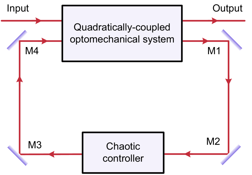
Figure 1: (Color online) Schematic diagram of the noise-decoupling system by coherent feedback modulation. Two quantum components, i.e., a quadratically-coupled optomechanical system and a chaotic controller, are connected by the mediated optical fields. The output of the optomechanical system is taken as the input fed into the chaotic controller. Also, the chaotic signal generated by the chaotic controller is then fed back to control the dynamics of the quadratically-coupled optomechanical system. The M1, M2, M3, M4 represent total-reflection mirrors that are introduced to change the light path. In this model, the radiation pressure can directly change the frequency of the mechanical resonator because the coupling between the mechanical mode and the optical mode is quadratic.

As illustrated in Fig. 1, our feedback control system consists of two components, i.e., a quadratically-coupled optomechanical system (the controlled system) and a chaotic controller. These two components are connected by a mediating optical field, from which we can construct a field-mediated coherent feedback system CF1 ; CF2 ; CF3 ; CF4 ; Jacobs . In the interaction picture of the noise frequency $\omega$, the Hamiltonian of the controlled device, i.e., the quadratically-coupled optomechanical device, can be written as QCS1 ; QCS2 ; QCS3 ; QCS4 ; QCS5

$$H_{1} = \omega_{a_{1}}a_{1}^{\dagger}a_{1}+G_{1}a_{1}^{\dagger}a_{1}b_{1}^{\dagger}b_{1}+\Omega_{1}b_{1}^{\dagger}b_{1}$$ (1)

$$+i\varepsilon_{1}\left[a_{1}^{\dagger}\exp({-i\omega_{d_{1}}t})-a_{1}\exp({i\omega_{d_{1}}t})\right]$$

$$+\sum_{\omega}g(\omega)\left[b^{\dagger}(\omega)b_{1}e^{-i\omega t}+b(\omega)b_{1}^{{\dagger}}e^{i\omega t}\right],$$

where $a_{1}$ and $b_{1}$ denote the annihilation operators of the cavity mode and the mechanical mode in the quadratically-coupled optomechanical system, and $\omega_{a_{1}}$, $\Omega_{1}$ are the natural frequencies of these two modes. Here, we assume that $\hbar=1$. The optomechanical coupling we consider here is a kind of quadratic optomechanical interaction with strength $G_{1}$ QCS1 ; QCS2 ; QCS3 ; QCS4 ; QCS5 . The optical mode $a_{1}$ is driven by an external driving field with strength $\varepsilon_{1}$ and frequency $\omega_{d_{1}}$. Here $b(\omega)$ represents the noise mode with frequency $\omega$ acting on the mechanical mode and $g({\omega})$ is the coupling strength between the mechanical mode and the noise mode.

Here we use $H_{c}$ to denote the Hamiltonian of the chaotic controller, and $a_{2}$ denotes the annihilation operator of the chaotic cavity field in the controller. Then the interaction Hamiltonian of the quadratically-coupled system and the controller $H_{\rm{int}}$ takes the form (see Appendix A)

$$H_{\rm{int}}=\frac{1}{2i}(\sqrt{\gamma_{1}\gamma_{2}}-\sqrt{\gamma_{2}\gamma_{f}})(a_{2}^{\dagger}a_{1}-a_{1}^{{\dagger}}a_{2}),$$ (2)

where $\gamma_{1}$ and $\gamma_{2}$ represent the damping rates of the optical cavities in the controlled system ”1” and the chaotic controller ”2”, and $\gamma_{f}$ denotes the damping rate of the controlled cavity induced by the feedback field. The total Hamiltonian of the coherent feedback loop is provided by

$$H_{\rm{tot}}=H_{1}+H_{c}+H_{\rm int}.$$ (3)

In the strong-driving regime, the optical fields in the quadratically-coupled optomechanical system and the chaotic controller can be treated classically. Here we replace the operator $a_{1}$ by $\alpha_{1}(t)$, which represents the classical part of the optical field $a_{1}$, and then eliminate the classical parts including $H_{c}$ and $H_{\rm int}$ in the total Hamiltonian. Thus the Hamiltonian of the feedback control system given in Eq. (3) can be simplified as

$$\begin{split}H_{\rm eff}=&\Omega_{1}{b_{1}}b_{1}^{\dagger}+f(t)\;b_{1}^{\dagger}b_{1}\\ &+\sum_{\omega}g({\omega})\left[{b({\omega})b_{1}^{\dagger}\exp({i\omega t})+\rm{h.c.}}\right],\end{split}$$ (4)

where $f(t)=G_{1}{|\alpha_{1}(t)|}^{2}$, and the amplitude of the cavity field $|\alpha_{1}(t)|$ is modulated by the chaotic controller and thus it is a broad-band signal. The effective Hamiltonian in Eq. (4) includes three parts: (i) the free Hamiltonian of the mechanical mode with natural frequency $\Omega_{1}$; (ii) a correction term with the mechanical frequency shift $f(t)$ induced by the chaotic controller $H_{c}$; (iii) the interaction Hamiltonian $H_{\rm int}$ between the mechanical mode $b_{1}$ and its environmental noises $b(\omega)$. In the rotating reference frame with the unitary operator

$$U=\exp\left[-{i}\int^{t}_{0}{\left(f(\tau)+\Omega_{1}\right)b_{1}^{\dagger}b_{1}}d\tau\right],$$ (5)

the effective Hamiltonian is given by

$$\tilde{H}_{\rm eff} = U^{\dagger}H_{\rm eff}U-iU^{{\dagger}}\partial{U}/\partial{t}$$

$$= \sum_{\omega}{g}(\omega)\left[b(\omega)b_{1}^{\dagger}e^{{-i(\Omega_{1}-\omega)t}-i\int_{0}^{t}{f(\tau)}d\tau}+{\rm h.c.}\right].$$

By averaging over the broadband signal $f(t)$ APS1 , we have (see Appendix B)

$$\overline{\exp\left[-i\int_{0}^{t}{f(\tau)}d\tau\right]}=\sqrt{M},$$ (7)

where $M$ is a correction factor. Thus, the effective Hamiltonian shown in Eq. (II) can be simplified as

$$\tilde{\tilde{H}}_{\rm eff}=\sum_{\omega}{\tilde{g}}({\omega})\left\{b({\omega})b_{1}^{\dagger}\exp[{-i(\Omega_{1}-\omega)t}]+{\rm h.c.}\right\},$$ (8)

where $\tilde{g}({\omega})=\sqrt{M}g({\omega})$ is the modified coupling strength between the mechanical mode and the heat bath after introducing the chaotic signal $f(t)$. It can be seen that the modified coupling strength $\tilde{g}(\omega)$ can be greatly decreased if the correction factor $M$ is small enough, under which the mechanical mode is efficiently decoupled from the environmental noises.

As shown in Appendix B, the correction factor $M$ is determined by the power spectrum $S_{f}(\omega)$ of the chaotic signal $f(t)$

$$M=\exp\left[-\pi\int^{\omega_{u}}_{\omega_{l}}\frac{S_{f}(\omega)}{\omega^{2}}d\omega\right],$$ (9)

where $\omega_{u}$ and $\omega_{l}$ are the upper bound and lower bound of the frequency band of the chaotic signal $f\left(t\right)$. Note that, $M$ varies from $0$ to $1$. Specially, $M=0$ corresponds to the full-decoupling case, and $M=1$ corresponds to the case without decoupling. Since the power spectrum $S_{f}(\omega)$ is broadened by the chaotic modulation, the value of $M$ is thus very small and the mechanical mode is decoupled from the environmental noises.

III Physical implementation in on-chip optomechanical systems

In this section, we discuss how to physically implement our chaotic-feedback-based noise decoupling strategy in on-chip optomechanical systems.

III.1 Implementation of the quadratically-coupled optomechanical system

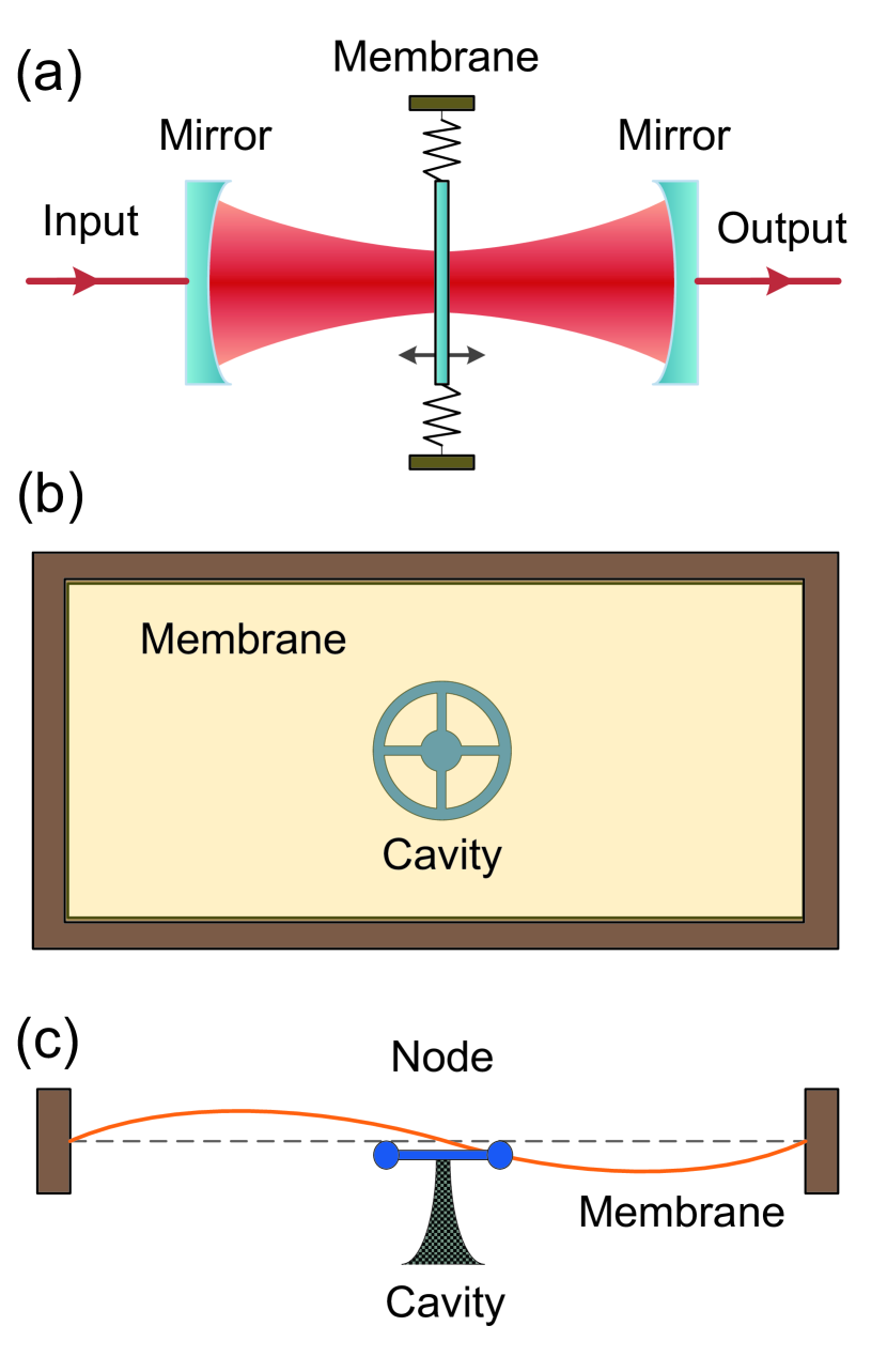
Figure 2: (Color online) Schematic diagram of the quadratic-coupling optomechanical systems with a Fabry-Perot cavity and the rectangular membrane. (a) Quadratic optomechanical system with a Fabry-Perot cavity: the quadratic-coupling is realized by putting a membrane in the middle of the Fabry-Perot cavity. (b) Top view and (c) cross-sectional view of a rectangular membrane optomechanical system, where its node coincides with the central point of the cavity. The rectangular membrane supports various vibrational modes $u=(j,k)$, where $j,k=1,2...$ are the mode indexes. Here the rectangular membrane is driven to the (1,2) mode, which has two anti-nodes and one node.

Here we list two possible examples of the quadratic-coupling optomechanical system QCS1 ; QCS2 ; QCS3 ; QCS4 ; QCS5 . The first example is shown in Fig. 2(a), in which a membrane is placed in the middle of a cavity and can move freely under the laser-induced pressure QCS1 ; QCS2 ; QCS3 ; QCS4 . Such kind of structure leads to a quadratic coupling term between the mechanical mode and the cavity mode. Another example for the quadratic-coupling is the rectangular membrane optomechanical system QCS5 . As seen in Figs. 2(b) and (c), the rectangular membrane placed above a toroidal cavity is driven by the optical field inside the toroidal cavity, which may generate both linear coupling and quadratic coupling modes between the cavity field and the membrane. The coupling strengthes of these two coupling modes are determined by three factors: (i) the vibrational mode of the rectangular membrane; (ii) the distance between the membrane and the upper surface of the toroidal cavity; and (iii) the relative position of the toroidal cavity. Moreover, the coupling modes displayed in the rectangular membrane optomechanical system can be controlled by modulating the above factors. The purely quadratic-coupling mode can be realized when QCS5 : (i) the rectangular membrane is excited in a vibrational mode that contains at least one node; (ii) the rectangular membrane is placed right above the toroidal cavity; and (iii) the node of the membrane is located at the central point of the cavity. Under these conditions, the linear coupling term between the membrane and the cavity field can be completely removed.

The mechanism of the rectangular membrane optomechanical system is similar to the Fabry-Perot-type quadratic-coupling system, and they share the same Hamiltonian, which is shown in Eq. (1). Hereafter, we apply our noise-decoupling method to the rectangular membrane optomechanical system presented above.

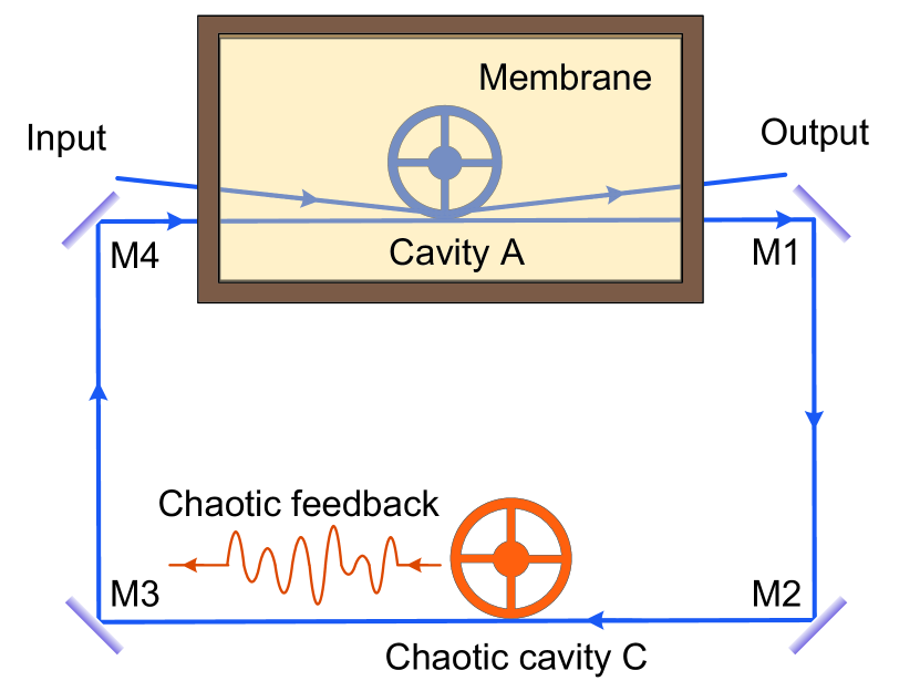
Figure 3: (Color online) The noise-decoupling model with the control of a toroidal cavity. Here the toroidal cavity is a chaotic controller, which shifts the cavity field of the quadratically-coupled optomechanical system to chaos.

III.2 Implementation of the chaotic controller

In this section, we consider an optomechanical system [see Fig. 3] with chaotic dynamics COM1 as the chaotic controller in the feedback control loop. For simplicity we denote the controlled quadratically-coupled optomechanical device as system $1$, and the chaotic controller as system $2$. The Hamiltonian of system $1$ is displayed in Eq. (1); and the Hamiltonian of system $2$ is taken as

$$\begin{split}H_{2}=&\omega_{a_{2}}a_{2}^{\dagger}a_{2}+G_{2}\,a_{2}^{\dagger}a_{2}(b_{2}^{\dagger}+b_{2})+\Omega_{2}\,b_{2}^{\dagger}b_{2}\\ &+i\varepsilon_{2}[a_{2}^{\dagger}\exp({-i\omega_{d_{2}}t})-{a_{2}}\exp({i\omega_{d_{2}}t})],\end{split}$$ (10)

where $a_{2}$ and $b_{2}$ denote the annihilation operators of the cavity mode and the mechanical mode in system $2$; and $\omega_{a_{2}}$, $\Omega_{2}$ correspond to their inherent frequencies. Here $G_{2}$ denotes the optomechanical coupling strength in system $2$. The cavity mode in system 2 is driven by an input laser field with driving strength $\varepsilon_{2}$ and corresponding driving frequency $\omega_{d_{2}}$. Here, the driving frequencies of the cavity modes in the two systems are chosen to be: $\omega_{d_{1}}=\omega_{d_{2}}=\omega_{d}$. In the rotating reference frame with the unitary operator $U=\exp[-i\omega_{d}(a_{1}^{{\dagger}}a_{1}+a_{2}^{{\dagger}}a_{2})t]$, the total Hamiltonian of the quantum feedback loop can be transformed to the form

$$\begin{split}H_{\rm{tot}}=&\Delta_{1}a_{1}^{\dagger}a_{1}+G_{1}a_{1}^{\dagger}a_{1}b_{1}^{\dagger}b_{1}+\Omega_{1}b_{1}^{\dagger}b_{1}\\ &+\Delta_{2}a_{2}^{\dagger}a_{2}+G_{2}a_{2}^{\dagger}a_{2}(b_{2}^{\dagger}+b_{2})+\Omega_{2}b_{2}^{\dagger}b_{2}\\ &+i\varepsilon_{1}(a_{1}^{\dagger}-{a_{1}})+i\varepsilon_{2}(a_{2}^{\dagger}-{a_{2}})\\ &+\frac{1}{2i}(\sqrt{\gamma_{1}\gamma_{2}}-\sqrt{\gamma_{2}\gamma_{f}})(a_{2}^{\dagger}a_{1}-a_{1}^{\dagger}a_{2})\\ &+\sum_{\omega}g(\omega)[b^{\dagger}(\omega)b_{1}\exp({-i\omega t})+\rm h.c.],\end{split}$$ (11)

where $\Delta_{1}=\omega_{a_{1}}-\omega_{d}$, and $\Delta_{2}=\omega_{a_{2}}-\omega_{d}$, denote the detuning frequencies of cavities $1$ and $2$. Here $\gamma_{1}$ and $\gamma_{2}$ represent the damping rates of the optical cavities $1$ and $2$, $\gamma_{f}$ denotes the damping rate induced by the feedback field of the controlled cavity. We use the quantum Langevin equations to describe the dynamics of the chaotic feedback system

$$\begin{split}\dot{a}_{1}=&-i\Delta_{1}a_{1}-\frac{1}{2}(\sqrt{\gamma_{1}}+\sqrt{\gamma_{f}})^{2}a_{1}-iG_{1}a_{1}b_{1}^{\dagger}b_{1}\\ &-\sqrt{\gamma_{2}\gamma_{f}}\,a_{2}+\varepsilon_{1}-(\sqrt{\gamma_{1}}+\sqrt{\gamma_{f}})a_{1,\rm in},\end{split}$$ (12a)

$$\begin{split}\dot{a}_{2}=&-i\Delta_{2}a_{2}-\frac{\gamma_{2}}{2}a_{2}-iG_{2}a_{2}(b_{1}^{\dagger}+b_{1})+\varepsilon_{2}\\ &-\sqrt{\gamma_{1}\gamma_{2}}\,a_{1}-\sqrt{\gamma_{2}}\,a_{2,\rm in},\end{split}$$ (12b)

$$\dot{b}_{1}=-i\Omega_{1}b_{1}-iG_{1}a_{1}^{\dagger}a_{1}{b_{1}}-\frac{\Gamma_{\!1}}{2}b_{1}-\sqrt{\Gamma_{\!1}}\,b_{1,\rm in},$$ (12c)

$$\dot{b}_{2}=-i\Omega_{2}b_{2}-iG_{2}a_{2}^{\dagger}a_{2}-\frac{\Gamma_{\!2}}{2}b_{2}-\sqrt{\Gamma_{\!2}}\,b_{2,\rm in},$$ (12d)

where $a_{1,\rm in}$ ($a_{2,\rm in}$) is the input of the optical cavity in system $1$ ($2$); $b_{1,\rm in}$ ($b_{2,\rm in}$) and $\Gamma_{\!1}$ ($\Gamma_{\!2}$) are the input and the damping rate of the mechanical mode in system $1$ ($2$). We assume that the backaction of the mechanical mode acting on the optical mode in system $1$ is very weak, then the evolution of the cavity mode $1$ mainly depends on Eqs. (12a), (12b), and (12d). In the strong-driving regime, the semiclassical approximation can be applied: $a_{1}=\alpha_{1}+\tilde{a}_{1}$, $a_{2}=\alpha_{2}+\tilde{a}_{2}$, and $b_{2}=\beta_{2}+\tilde{b}_{2}$, where $\alpha_{1}$, $\alpha_{2}$, and $\beta_{2}$ represent the classical parts and $\tilde{a}_{1}$, $\tilde{a}_{2}$ and $\tilde{b}_{2}$ denote the operators for the quantum fluctuations. Then we neglect the quantum fluctuation terms in Eqs. (12a), (12b), and (12d). Thus the evolution of the classical parts in the total system can be described by

$$\begin{split}\dot{\alpha}_{1}=&-i\Delta_{1}\alpha_{1}-\frac{1}{2}(\sqrt{\gamma_{1}}+\sqrt{\gamma_{f}})^{2}\alpha_{1}\\ &\varepsilon_{1}-\sqrt{\gamma_{2}\gamma_{f}}\,\alpha_{2},\end{split}$$ (13a)

$$\begin{split}\dot{\alpha}_{2}=&-i\Delta_{2}\alpha_{2}-\frac{\gamma_{2}}{2}\alpha_{2}-iG_{2}\alpha_{2}(\beta_{2}^{\ast}+\beta_{2})\\ &+\varepsilon_{2}-\sqrt{\gamma_{1}\gamma_{2}}\,\alpha_{1},\end{split}$$ (13b)

$$\dot{\beta}_{2}=-i\Omega_{1}\beta_{2}-iG_{2}\alpha_{2}^{\ast}\alpha_{2}-\frac{\Gamma_{\!2}}{2}\beta_{2}.$$ (13c)

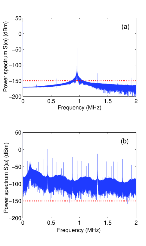
Figure 4: (Color online) Power spectra of the mechanical mode in system $1$: (a) without feedback and (b) with the chaotic feedback is applied. (a) the mechanical membrane is driven by a period signal; (b) we use a chaotic controller (optomechanical system in this case) to modulate the power of the mechanical membrane to a wide region. The parameters are set as follows: $\Delta_{1}/{2\pi}=0.75~{}\rm GHz$, $\Delta_{2}/2\pi=0.12~{}\rm GHz$, $\gamma_{1}/2\pi=1~{}\rm MHz$, $\gamma_{2}/2\pi=0.24~{}\rm GHz$, $\gamma_{f}/2\pi=0.05~{}\rm MHz$, $\Gamma_{\!1}/2\pi=0.01~{}\rm MHz$, $\Gamma_{\!2}=/2\pi=1.4~{}\rm MHz$, $\Omega_{1}/2\pi=1~{}\rm MHz$, $\Omega_{2}/2\pi=0.345~{}\rm GHz$, $G_{1}/2\pi=0.1~{}\rm MHz$, $G_{2}/2\pi=0.1~{}\rm MHz$, $\varepsilon_{1}/2\pi=6.6~{}\rm GHz$, and $\varepsilon_{2}/2\pi=13.2~{}\rm GHz$.

When the strength of the driving field $\varepsilon_{2}$ is strong enough, the optomechanical system $2$ enters the chaotic regime and will have a broadband cavity spectrum. As the chaotic controller, system $2$ can spread the spectrum of system $1$ both in the cavity mode and in the mechanical mode. Figure. 4 shows the spectrum of the mechanical mode in system $1$ without [Fig. 4(a)] and with [Fig. 4(b)] the feedback modulation. As shown in Fig. 4(a), only a single peak with very small sidebands is displayed in the spectrum of the mechanical mode if we do not introduce any feedback modulation. The power of the background frequency components is very small (less than -150 dBm). This corresponds to the periodic case. After we introduce the chaotic feedback [see Fig. 4(b)], the spectrum of the controlled mechanical mode is greatly broadened and the whole baseline of the spectrum is increased to above $150$ dBm. This corresponds to the chaotic case, and the broadband response of the mechanical mode will decouple the mechanical mode from the environmental noises.

As discussed in Sec. ii@, we use the factor $M$ to evaluate the efficiency of our noise decoupling strategy [see Eq. (9)]. The value of $M$ is determined by the spectrum $S_{f}{(\omega)}$ of the signal $f(t)$ (recall that $f(t)=G_{1}{|\alpha_{1}(t)|}^{2}$), which can be obtained by numerically solving Eq. (13). Note that $M\sim 1$ when the spectrum $S_{f}{(\omega)}$ is concentrated in a narrow region, and $M$ will be close to zero if the spectrum $S_{f}\left(\omega\right)$ is broadened by the chaotic modulation. In our numerical simulations, we find that $M\approx 1$ if we do not introduce feedback [Fig. 4(a)] and $M=0.0074$ if we introduce the chaotic feedback [Fig. 4(b)], which coincides with what we expect.

IV Storage of continuous-variable quantum information

The storage of continuous-variable quantum information, i.e., to realize continuous-variable quantum memory QM1 ; QM2 ; QM3 ; QM5 ; QM7 ; QM8 , is important for quantum communications and quantum computation. One possible way to solve this problem is to transfer the continuous-variable information in the optical signal to an on-chip mechanical resonator which has a lower damping rate. The continuous-variable optomechanical quantum memory system we consider here is presented in Fig. 5, which includes the input (output) fields, an optical cavity, and a mechanical resonator QM2 . By exchanging states, between the cavity mode and the mechanical mode, a quantum state carried by the input field can be written into and stored in the nanomechanical resonator.

However, the quantum information stored in the mechanical resonator will unavoidably be destroyed due to the coupling between the mechanical resonator and the environmental noise. Thus, to realize such kind of continuous-variable quantum memory, we have to suppress the decoherence effects of the mechanical mode induced by the environmental noise. As we have discussed in the previous sections, introducing a chaotic coherent feedback loop to drive the mechanical mode into the broad-band regime is an efficient way to decouple the mechanical mode from the environmental noise. In this section, we will show how to use this noise-decoupled nano-mechanical resonator as a quantum memory.

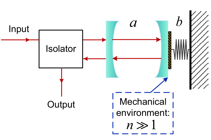
Figure 5: (Color online) Schematic diagram of an optmechanical system for quantum information transfer and storage. A beam of light with a desirable quantum state is fed into a cavity, and then transferred to the mechanical resonator. Here $a$ is the cavity mode and $b$ denotes the mechanical mode, $n$ represents the mean thermal excitation phonon number which follows the Boltzmann distribution.

Our purpose here is to use a noise-decoupled mechanical resonator to store continuous-variable information. The key point is how to transfer a quantum state to a mechanical mode and decouple this mechanical mode simultaneously. Here we propose a strategy with two optical cavities sharing the same mechanical resonator but with different optomechanical coupling: one is with linear optomechanical coupling used for quantum memory; and the other is with a quadratic optomechanical coupling, used for noise decoupling.

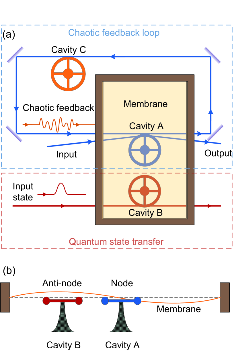
Figure 6: (Color online) (a) Top view of the quantum memory system. The noise-decoupled quantum memory system can be divided into two parts shown by the dashed rectangular grid frames: the chaotic feedback loop (inside the blue frame) for the noise decoupling of the rectangular membrane; the setup used for transferring the quantum state (the red frame) from the input light to the noised-decoupled rectangular membrane. (b) Cross-sectional side view of the rectangular membrane optomechanical system. Cavity A is placed at the node of the rectangular membrane, and cavity B is placed at the anti-node.

Let us now consider how to apply this quantum memory model in the rectangular membrane optomechanical system proposed in Ref. QCS5 . Figure 6(a) shows two toroidal cavities (A and B) connected to a rectangular membrane. The types of coupling between the cavity mode and the mechanical mode are determined by the positions they are placed: the node of the membrane corresponds to a linear coupling and the anti-node corresponds to a quadratic coupling [Fig. 6(a)]. Thus, we place the toroidal cavity (cavity A) used for noise decoupling at the node of the membrane; and the other toroidal cavity (cavity B), used for quantum memory, at the anti-node. Toroidal cavity A is modulated by the chaotic controller (toroidal cavity C), which leads to the decoupling between the membrane and its environmental noises. The cavity B is used for storing the quantum state in the membrane. The coupling between the cavity mode and the mechanical mode is assumed to be linear under the strong-driving regime QM1 ; QM2 . Thus, the Hamiltonian of the total system can be written as

$$\begin{split}H=&\Delta_{s}a_{s}^{\dagger}a_{s}+G_{s}(a_{s}b_{1}^{\dagger}+a_{s}^{\dagger}b_{1})\\ &+(\Omega_{1}+G_{1}{|\alpha_{1}(t)|}^{2}){b_{1}}^{\dagger}b_{1}\\ &+\sum_{\omega}g({\omega})[b^{\dagger}(\omega)b_{1}\exp({-i\omega t})+\rm h.c.],\end{split}$$ (14)

where $a_{s}$ ($a_{s}^{{\dagger}}$) represents the annihilation (creation) operator of the optical mode in cavity $B$, and $\omega_{s}$ is the corresponding inherent frequency. Here $\Delta_{s}=\omega_{s}-\omega_{d}$ is the detuning frequency of cavity $B$, and $\omega_{d}$ is the frequency of the external driving field. Also, $G_{s}$ denotes the coupling strength between the optical mode and the mechanical mode. To compensate the effect induced by the chaotic feedback on the quantum memory system, we take the detuning frequency as $\Delta_{s}=\Omega_{1}+G_{s}{|\alpha_{1}(t)|}^{2}$. In the rotating reference frame with the unitary matrix

$$U=\exp\left[-{i}\int^{t}_{0}{(G_{1}{|\alpha_{1}(\tau)|}^{2}+\Omega_{1})(b_{1}^{\dagger}b_{1}+a_{1}^{\dagger}a_{1})}d\tau\right],$$ (15)

the effective system Hamiltonian can be represented by

$${H}_{\rm eff}=G_{s}(a_{s}^{{}^{\dagger}}b_{1}+a_{s}b_{1}^{{}^{\dagger}})+\sum_{\omega}{\tilde{g}({\omega})}[b^{\dagger}(\omega)b_{1}e^{-i(\Omega_{1}-\omega)t}+\rm h.c.],$$ (16)

where $\tilde{g}({\omega})=\sqrt{M}g({\omega})$ and $M$ is the decoupling factor. After introducing the adiabatic approximation to eliminate the cavity mode shown in Ref. QM2 , we use $\tilde{b}_{1}$ to denote the annihilation operator of the mechanical mode and the quantum Langevin equation of the optomechanical system can be simplified as

$$\frac{d\tilde{b}_{1}}{dt}=-\frac{\nu+\Gamma_{\!1}}{2}\tilde{b}_{1}-\sqrt{\nu}\,{a_{d}}-\sqrt{\Gamma_{\!1}}\,b_{\rm in}(t),$$ (17)

${a}_{d}$ denotes the optical field fed into cavity $B$. Let ${a}_{d}=\alpha_{d}+\tilde{a}_{d}$, where $\alpha_{d}$ and $\tilde{a}_{d}$ denote the classical part and the quantum fluctuation of the optical mode. The fluctuation terms $\tilde{a}_{d}$ and $b_{\rm in}$ satisfy the relations: $\langle{\tilde{a}_{d}(t)\tilde{a}_{d}^{{\dagger}}(t^{{}^{\prime}})}\rangle=\delta(t-t^{{}^{\prime}})$, $\langle{{b}_{\rm in}(t){b}_{\rm in}^{{\dagger}}(t^{{}^{\prime}})}\rangle=(n+1)\delta(t-t^{{}^{\prime}})$, where $n\left(\Omega_{1}\right)\approx k_{B}T/\hbar\Omega_{1}$ is the mean thermal excitation phonon number. The parameter $\nu$ in Eq. (17) can be calculated by $\nu={(G_{s}|\alpha_{d}|)^{2}}/{\gamma_{s}}$, where $G_{s}$ is the coupling strength between the mechanical mode and the optical mode, and $\gamma_{s}$ is the damping rate of the optical mode QM1 .

We now assume that the system is initially in a Gaussian state. We use the fidelity $F_{\infty}$ between the initial state and the steady state of the mechanical mode to characterize the efficiency of noise decoupling, which can be calculated by QM1

$$\begin{split}F_{\infty}=&\langle{\Psi_{0}}|{\rho_{\infty}}|{\Psi_{0}}\rangle\\ =&\prod_{j=\pm s}\left[\exp({j})+\frac{\Gamma_{\!1}(2n+1-\exp({j}))}{2(\nu+\Gamma_{\!1})}\right]^{-\frac{1}{2}}.\end{split}$$ (18)

Here $s$ is the squeezing factor (see Appendix C). The steady-state fidelity $F_{\infty}$ mainly depends on four factors: the mean thermal excitation phonon number $n$, the coupling strength $\nu$, the squeezing factor $s$, and the mechanical damping rate $\Gamma_{\!1}$. We can see that the fidelity $F_{\infty}$ can be increased by decreasing the mechanical damping rate $\Gamma_{\!1}$, and, as shown in Sec. ii@, $\Gamma_{\!1}$ can be reduced by introducing a chaotic feedback loop. In fact, after introducing the chaotic feedback control, the effective damping rate of the mechanical mode is given by

$$\Gamma_{1}^{\prime}=M\Gamma_{\!1}.$$ (19)

Thus the modified fidelity $F_{\infty}^{\prime}$ can be written as

$$F_{\infty}^{\prime}=\prod_{j=\pm s}\left[\exp({j})+\frac{\Gamma_{1}^{\prime}(2n+1-\exp({j}))}{2(\nu+\Gamma_{1}^{\prime})}\right]^{-\frac{1}{2}}.$$ (20)

When the controller in the feedback loop enters the chaotic regime, we have $\Gamma_{1}^{\prime}\approx 0$, and thus $F_{\infty}^{\prime}\approx 1$, which means almost perfect quantum state transfer.

Then, we numerically calculate the steady-state fidelity $F_{\infty}$ between the input state and the steady state of the mechanical resonator. Two different Gaussian input states are considered: coherent states and squeezed states.

IV.1 Coherent input state

In this subsection, we consider the quantum mechanical memory system with a coherent input state. For a coherent input state, the squeezing factor $s=0$. Thus, in this case, the fidelity $F_{\infty}^{c}$ can be simplified as

$$F_{\infty}^{c}=\left[1+\frac{\Gamma_{\!1}n}{\nu+\Gamma_{\!1}}\right]^{-1}.$$ (21)

By comparing the fidelity between the input state and the steady state of the mechanical mode (under the noise-decoupling control [see Fig. 7(a)] and without the noise-decoupling control [see Fig. 7(b)]), we find remarkable improvement of the efficiency of the quantum memory by introducing chaotic control. From Fig. 7(a) and Fig. 7(b), we can observe that the decrease of the mean thermal excitation phonon number $n$ or the increase of the parameter $\nu$ would lead to the improvement of the fidelity of the quantum transfer. If we fix the parameter $\nu=50$ kHz, the fidelity of the quantum transfer will fall to zero rapidly when increasing the excitation phonon number $n$ without introducing the noise-decoupling control [Fig. 7(a)]. We find that the fidelity of the quantum memory is increased and approaches one even when the mean thermal excitation phonon number $n$ exceeds $10^{5}$ after introducing the noise-decoupling control. This means that our noise-decoupling method efficiently reduces the damping rate of the mechanical mode $\Gamma_{\!1}$, and thus protects the coherent input state from decoherence.

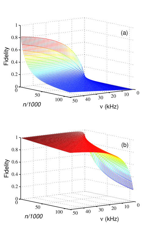
Figure 7: (Color online) The fidelity (a) before the noise decoupling and (b) after the noise decoupling. Here $n$ is the mean thermal excitation phonon number which follows the Boltzmann distribution, and $\nu$ is a parameter related to the optomechanical coupling strength. The parameters are: $\Omega_{1}/2\pi=1$ MHz, $\Gamma_{\!1}/2\pi=5$ Hz for (a), and $\Gamma_{1}^{\prime}/2\pi=0.037$ Hz for (b).

IV.2 Squeezed input state

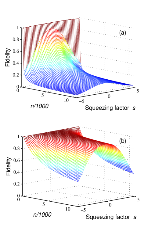
Figure 8: (Color online) The fidelity (a) before noise decoupling and (b) after noise decoupling. The parameters used are: $\nu/2\pi=10~{}\rm kHz$, $\Gamma_{1}/2\pi=5~{}\rm Hz$ for (a), and $\Gamma_{1}^{\prime}/2\pi=0.037~{}\rm Hz$ for (b). The natural frequency of the mechanical mode is assumed as $\Omega_{1}/2\pi=1~{}\rm{MHz}$.

Let us consider the case that the input state is a squeezed state with squeezing factor $s\neq 0$. By adjusting the squeezing factor $s$ and the mean thermal excitation phonon number $n$, we study the fidelity between the input squeezed state and the steady state of the mechanical mode.

Compared to case without noise-decoupling control shown in Fig. 8(a), the fidelity under noise-decoupling control is significantly improved [see Fig. 8(b)] for different chosen system parameters. As shown in Fig. 8(a) and (b), the fidelity decreases when increasing the squeezing factor $s$ and the mean thermal excitation phonon number $n$. Here we vary the squeezing factor $s$ from $-5$ to $5$, and it can be found that the curve of fidelity is symmetrical about the plane $s=0$ in the three-dimensional fidelity space. For each parameter $n$, the fidelity is maximized when $s=0$, which corresponds to the case that the input state is a coherent state. The quantum information stored in the memory system is more likely to be damaged by the heat bath when increasing the degree of the squeezing factor $s$. As shown in Fig. 8, the fidelity of quantum transfer $F=0.16$ is very low when $n=10^{5}$ and $s=0$ without the noise-decoupling control [see Fig. 8(a)], while, with the same condition, the fidelity is enhanced to be $F=0.96$ if we introduce the noise-decoupling control [see Fig. 8(b)]. When the squeezing factor $s$ is increased to approach $5$, the fidelity decreases to zero rapidly without the noise-decoupling control [see Fig. 8(a)], while it will remain nonzero, i.e., $F=0.38$, when we introduce the noise-decoupling control [see Fig. 8(b)].

V Conclusion

To summarize, by introducing a chaotic feedback control loop, we propose a strategy to decouple a nanomechanical resonator in a quadratically-coupled optomechanical system from the environmental noises. The main advantage of this method is to introduce a chaotic controller to significantly broaden the spectrum of a mechanical resonator and thus efficiently suppress the environmental noise. As an application, we study this proposed the noise-decoupled nanomechanical resonator under chaotic coherent feedback control as a quantum memory to store the information transferred from external optical signals. Two different input states, i.e., coherent and squeezed states, are studied to show the efficiency of the quantum memory. The numerical results show that the fidelity of the quantum memory has been greatly improved after introducing our noise-decoupling strategy. We believe that this nonlinear coherent feedback strategy will have various applications, such as nonlinear modulation of photon transport and high-sensitivity quantum measurements, which will be considered in future work.

Appendix A Theory of Markovian coherent feedback network

To study the multi-channel quantum input-output network, we now introduce the $SLH$ method presented in Ref. SLH . In the $SLH$ language, an open quantum system can be fully characterized by $G=(S,L,H)$, where $S$ denotes a $n\times n$ unitary scattering matrix, which satisfies $SS^{{\dagger}}=S^{{\dagger}}S=I$, $L$ represents the dissipation operator which is determined by the dissipation channels induced by the input fields, and $H$ is the free Hamiltonian of the system. Within the framework of $G=(S,L,H)$, the quantum Langevin equation of an arbitrary system operator $X$ is given by

$$\begin{split}\dot{X}=&-i[X,H_{\rm sys}]+\{L^{\dagger}[X,L]+[L^{\dagger},X]L\}/2\\ &+\{b_{\rm in}[L^{\dagger},X]+[X,L]b_{\rm in}^{\dagger}\}.\end{split}$$ (22)

The $SLH$ method provides a convenient way to study the all-optical quantum coherent forward and feedback networks SLH . For example, we show in Fig. 9 two quantum components: $G_{1}=(S_{1},L_{1},H_{1})$ and $G_{2}=(S_{2},L_{2},H_{2})$. The series product of these two components can be parameterized by

$$G_{2}\triangleright G_{1} = [S_{2}S_{1},L_{2}+S_{2}L_{1},$$ (23)

$$H_{1}+H_{2}+\frac{1}{2i}(L_{2}^{{\dagger}}S_{2}L_{1}-L_{1}^{{\dagger}}S_{2}^{{\dagger}}L_{2})].~{}$$

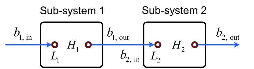
Figure 9: (Color online) Schematic diagram of the series product of two cascaded-connected components.

A typical coherent feedback control system is shown in Fig. 10, which is composed of the controlled system, i.e., system $1$, and the controller, i.e., system $2$. This coherent feedback control system can be seen as a series product of three components: $G_{1}=(S_{1},L_{1},H_{1})$, $G_{2}=(S_{2},L_{2},H_{2})$, and $G_{f}=(S_{f},L_{f},H_{1})$. Thus, the corresponding $SLH$ parameters of this feedback control system can be represented by

$$G_{f}\triangleright G_{2}\triangleright G_{1} = (S,L,H_{\rm sys}),$$ (24)

where

$$S=S_{f}S_{2}S_{1},\ \ \ \ L=S_{2}S_{1}L_{1}+S_{1}L_{2}+L_{f},$$ (25a)

$$H_{\rm sys}=H_{1}+H_{2}+H_{\rm int},$$ (25b)

and the interaction Hamiltonian induced by the coherent feedback loop is given by

$$\begin{split}H_{\rm{int}}=&\frac{1}{2i}(L_{2}^{\dagger}S_{2}L_{1}-L_{1}^{\dagger}S_{2}^{{\dagger}}L_{2}\\ &+L_{f}^{\dagger}S_{f}L_{2}-L_{2}^{\dagger}S_{f}^{{\dagger}}L_{f}+L_{f}^{\dagger}S_{f}S_{2}L_{1}-L_{1}^{\dagger}S_{2}^{{\dagger}}S_{f}^{{\dagger}}L_{f}).\end{split}$$ (26)

As an example, let us consider our feedback-induced noise-decoupling system. As introduced in section $3$, a quadratically-coupled optomechanical device (system $1$) and a chaotic controller (system $2$) are connected by optical fields to construct a coherent feedback loop, which is similar to that given by Eq. (25). Let $a_{1}$ ($a_{2}$) be the annihilation operator of the cavity mode in quantum system $1$ ($2$) with corresponding damping rate $\gamma_{1}$ ($\gamma_{2}$), and $\gamma_{f}$ is the damping rate of the controlled cavity induced by the feedback field. In this case, we have $L_{1}=\sqrt{\gamma_{1}}\,a_{1}$, $L_{2}=\sqrt{\gamma_{2}}\,a_{2}$, and $L_{f}=\sqrt{\gamma_{f}}\,a_{1}$, and $S_{1}=S_{2}=S_{f}=I$. From Eq. (26), the dissipation operator of the total feedback loop can be written as

$$L=(\sqrt{\gamma_{1}}+\sqrt{\gamma_{f}})a_{1}+\sqrt{\gamma_{2}}\,a_{2},$$ (27)

and the total Hamiltonian of the quantum feedback loop can be obtained from Eq. (25) and Eq. (26) as

$$\begin{split}H_{\rm sys}&=H_{1}+H_{2}+H_{\rm int}\\ &=H_{1}+H_{2}+\frac{1}{2i}(\sqrt{\gamma_{1}\gamma_{2}}-\sqrt{\gamma_{2}\gamma_{f}})(a_{2}^{\dagger}a_{1}-a_{1}^{{\dagger}}a_{2}).\end{split}$$ (28)

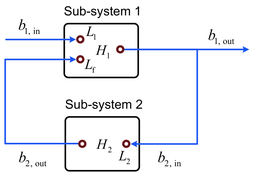
Figure 10: (Color online) Schematic diagram of a coherent feedback loop.

Accordingly, the quantum Langevin equations of the two cavity modes $a_{1}$ and $a_{2}$ can be represented by

$$\begin{split}\dot{a}_{1}=&-i[a_{1},H_{1}+H_{2}]-\frac{1}{2}(\sqrt{\gamma_{1}}+\sqrt{\gamma_{f}})^{2}a_{1}\\ &-\sqrt{\gamma_{2}\gamma_{f}}\,a_{2}-(\sqrt{\gamma_{1}}+\sqrt{\gamma_{f}})\,a_{1,\rm in},\end{split}$$ (29a)

$$\begin{split}\dot{a}_{2}=-i[a_{2},H_{1}+H_{2}]-\frac{\gamma_{2}}{2}a_{2}-\sqrt{\gamma_{1}\gamma_{2}}\,a_{1}-\sqrt{\gamma_{2}}\,a_{2,\rm in},\end{split}$$ (29b)

where $a_{1,\rm in}$ ($a_{2,\rm in}$) is the input field fed into the system $1$ ($2$). By substituting Eqs. (1) and (10) into Eq. (29), we can obtain the quantum Langevin equation given by Eq. (12).

Appendix B Derivation of the decoupling coefficient $M$

The decoupling coefficient $M$ is determined by the classical cavity field $f(t)$, which can be decomposed into a series of frequency components by the Fourier transform DC1 ; APS1 .

$$f(t)=\sum^{\infty}_{n=0}A_{n}\cos(\omega_{n}t+\varphi_{n}),$$ (30)

where $\omega_{n}$, $A_{n}$ and $\varphi_{n}$ denote the frequency, the amplitude and the initial phase of the $n$-th frequency components. Integrating $f(t)$ gives the control-induced phase shift

$$\theta(t)=\int_{0}^{t}\!\!f(\tau)\;d\tau=\sum_{n=0}^{\infty}\frac{A_{n}}{\omega_{n}}\sin(\omega_{n}t+\varphi_{n}).$$ (31)

By introducing the Bessel-series expansion, we have

$$\begin{split}\exp\left[-i\theta(t)\right]&=\exp\left[-i\sum_{n=0}^{\infty}\frac{A_{n}}{\omega_{n}}\sin(\omega_{n}t+\varphi_{n})\right]\\ &=\prod_{\alpha}\sum_{n}J_{n\alpha}\left(\frac{A_{\alpha}}{\omega_{\alpha}}\right)\exp[-in_{\alpha}\omega_{\alpha}t-in_{\alpha}\varphi_{\alpha}],\end{split}$$ (32)

where $J_{n\alpha}$ is the $n$-th Bessel function of the first kind. We then neglect the high-order terms in Bessel series, which can be considered as the fast variables in the system, and only keeps the zero-order terms in Eq. (32), by which we have

$$\overline{\exp(-i\theta(t))}=\prod_{\alpha}J_{0}\left(\frac{A_{\alpha}}{\omega_{\alpha}}\right)=\exp\left[\sum_{\alpha}\ln{J_{0}}\left(\frac{A_{\alpha}}{\omega_{\alpha}}\right)\right].$$ (33)

Under the condition that $A_{\alpha}\ll\omega_{\alpha}$, the zero-order Bessel term can be approximately expressed as $J_{0}({A_{\alpha}}/{\omega_{\alpha}})\approx 1-{({A_{\alpha}}/2{\omega_{\alpha}})^{2}}$. Furthermore, from $A_{\alpha}\ll\omega_{\alpha}$, we have $\ln(1-({A_{\alpha}}/2{\omega_{\alpha}})^{2})\approx-({A_{\alpha}}/2{\omega_{\alpha}})^{2}$. Thus Eq. (33) can be simplified as

$$\prod_{\alpha}J_{0}\left(\frac{A_{\alpha}}{\omega_{\alpha}}\right) = \exp{\left[-\frac{1}{4}\sum_{\alpha}{\frac{A_{\alpha}^{2}}{\omega_{\alpha}^{2}}}\right]}$$ (34)

$$= \exp{\left[-\frac{\pi}{2}\int_{\omega_{l}}^{\omega_{u}}{\frac{S_{f}(\omega)}{\omega_{\alpha}^{2}}d\omega}\right]}.$$

Let $\sqrt{M}=\overline{\exp(-i\theta(t))}$, and $M$ is defined as the decoupling factor, then from Eq. (34) we have

$$M=\exp{\left[-{\pi}\int_{\omega_{l}}^{\omega_{u}}{\frac{S_{f}(\omega)}{\omega_{\alpha}^{2}}d\omega}\right]}.$$ (35)

Appendix C fidelity of the quantum memory

The Langevin equation of the mechanical operator $\tilde{b}_{1}$ is shown in Eq. (17). The steady value of the mechanical mode can be obtained by setting ${d\tilde{b}_{1}}/{dt}=0$ as

$$\langle{{\tilde{b}_{1}}(\infty)}\rangle=\frac{-2\sqrt{\nu}}{\nu+\Gamma_{\!1}}\alpha_{d},$$ (36)

where $\langle\cdot\rangle$ is the average over the input vacuum fluctuation. We then define the quantum Wiener processes $A(t)=\int_{0}^{t}{\tilde{a}_{d}(t^{{}^{\prime}})}d{t^{{}^{\prime}}}$, $B(t)=\int_{0}^{t}{{b_{\rm in}}(t^{{}^{\prime}})}d{t^{{}^{\prime}}}$, by which we can obtain the quantum stochastic differential equation from Eq. (17) as

$$d{\tilde{b}}_{1}=-\frac{\nu+\Gamma_{1}}{2}\,\tilde{b}_{1}{dt}-\sqrt{\nu}\,\alpha_{d}{dt}-\sqrt{\nu}\,d\!A-\sqrt{\Gamma_{1}}d\!B.$$ (37)

The quantum fluctuation terms $d\!A$ and $d\!B$ satisfy that

$$\langle d\!A\rangle=\langle d\!B\rangle=0,$$ (38)

and obey the quantum Ito rules

$$\!\!\!\!\!\!\!\!\!\!\!\!\!\!\!\!d\!A\;d\!A^{{\dagger}}=(N+1)dt,\ \ \ d\!A^{{\dagger}}d\!A=N\,dt,$$

$$\!\!\!\!\!\!\!\!\!\!\!\!\!\!\!\!(d\!A)^{2}=M\,dt,\ \ \ (d\!A^{{\dagger}})^{2}=M^{{\dagger}}dt,$$ (39)

$$\!\!\!\!\!\!\!\!\!\!\!\!\!\!\!\!d\!B\;d\!B^{{\dagger}}=(n+1)dt,\ \ \ d\!B^{{\dagger}}d\!B=n\,dt,$$

where $n$ represents the thermal excition number, $N$ is the effective photon number, and $M$ denotes the squeezing parameter. Here $M$ and $N$ satisfy the inequality $M^{2}\geq N(N+1)$. Then we introduce the squeezing factor $s$ QO of the input quantum state, which is given by

$$s=\ln{\left[M+M^{*}+2N+1\right]}.$$ (40)

To calculate the fidelity of the quantum memory, let us define the normalized position $x=(\tilde{b}_{1}+\tilde{b}^{{\dagger}}_{1})/\sqrt{2}$, momentum $p=(\tilde{b}_{1}-\tilde{b}^{{\dagger}}_{1})/\sqrt{2}i$, and the conjugate vector $\textbf{z}=(x,p)$ of the mechanical mode. We also introduce the symmetrized covariance matrix $V$, which is given by

$$V=\frac{1}{2}[\Delta\textbf{z}\ \Delta\textbf{z}^{\textrm{T}}+(\Delta\textbf{z}\ \Delta\textbf{z}^{\textrm{T}})^{\textrm{T}}],$$ (41)

where $\Delta\textbf{z}=\textbf{z}-\langle\textbf{z}\rangle$. With Ito’s rule $d(ab)=(da)b+a(db)+da\,db$, the time evolution of the covariance matrix $V$ is described by the Lyapunov differential equation

$$\dot{V}=AV+VA^{T}+\Gamma_{1}(n+1/2)I_{2}+\nu\,\Lambda,$$ (42)

where $A=-\left[(\nu+\Gamma_{1})/2\right]I_{2}$, and $I_{2}$ is the two-dimensional identity matrix. Here, $\Lambda$ is a matrix related to the degree of squeezing, which can be calculated by

$$\Lambda=\frac{1}{2}\left(\begin{array}[]{cc}{2N+1+M+M^{*}}&{M-M^{*}}\\ {M-M^{*}}&{2N+1-(M+M^{*})}\end{array}\right).$$ (43)

For a squeezed input state, the fidelity between the initial state and the steady state of the mechanical mode is given by

$$\begin{split}F_{\infty}=&\langle{\Psi_{0}}|{\rho_{\infty}}|{\Psi_{0}}\rangle=\frac{1}{\sqrt{\det(V_{\infty}+V_{0})}}\\ =&\prod_{j=\pm s}\left[\exp{(j)}+\frac{\Gamma_{1}(2n+1-\exp{(j)})}{2(\nu+\Gamma_{\!1})}\right]^{-\frac{1}{2}},\end{split}$$ (44)

where $V_{\infty}$ denotes the stationary solution of the Lyapunov differential equation [Eq. (42)] and $V_{0}$ is the covariance matrix of the input state, which can be calculated by

$$V_{0}=\frac{1}{2}\left(\begin{array}[]{cc}\exp{(s)}&0\\ 0&\exp{(-s)}\end{array}\right).$$ (45)

When the input state is a coherent state, such that $M\,=\,N\,=\,0$ and thus $s\,=\,0$, the fidelity in this case can be simplified as

$$\begin{split}F_{\infty}^{c}=\frac{1}{\sqrt{\det(V_{\infty}+V_{0})}}\\ =\left[1+\frac{\Gamma_{\!1}n}{\nu+\Gamma_{\!1}}\right]^{-1}.\end{split}$$ (46)

It can be found from Eqs. (44) and (46) that the fidelity increases when increasing the mechanical damping rate $\Gamma_{1}$ for both squeezed states and coherent states.

References

- (1) M. Aspelmeyer, T. Kippenberg, and F. Marquardt, Rev. Mod. Phys. 86, 1391 (2014).
- (2) F. Marquardt and S. M. Girvin, Physics 2, 40 (2009).
- (3) T. J. Kippenberg and K. J. Vahala, Opt. Express 15, 17172 (2007).
- (4) W. Lechner, S. J. M. Habraken, N. Kiesel, M. Aspelmeyer, and P. Zoller, Phys. Rev. Lett. 110, 143604 (2013).
- (5) T. H. Lee, S. Bhunia, and M. Mehregany, Science 329, 1316 (2010).
- (6) I. Buluta and F. Nori, Science 326, 108 (2009).
- (7) G. D. Cole and M. Aspelmeyer, Nature Nanotech. 6, 690 (2011).
- (8) I. M. Georgescu, S. Ashhab, and F. Nori, Rev. Mod. Phys. 86, 153 (2014).
- (9) H. Jing, S. K. Ozdemir, X. Y. Lü, J. Zhang, L. Yang, and F. Nori, Phys. Rev. Lett. 113, 053604 (2014).
- (10) X. Y. Lü, W. M. Zhang, S. Ashhab, Y. Wu, and F. Nori, Sci. Rep. 3, 2943 (2013).
- (11) I. Buluta, S. Ashhab, and F. Nori, Rep. Prog. Phys. 74, 104401 (2011).
- (12) J. D. Teufel, T. Donner, D. Li, J. W. Harlow, M. S. Allman, K. Cicak, A. J. Sirois, J. D. Whittaker, K. W. Lehnert, and R. W. Simmonds, Nature 475, 359 (2011).
- (13) E. Verhagen, S. Deleglise, S. Weis, A. Schliesser, and T. J. Kippenberg, Nature 482, 63 (2012).
- (14) X. W. Xu, Y. J. Zhao, and Y. X. Liu, Phys. Rev. A 88, 022325 (2013).
- (15) X. W. Xu, H. Wang, J. Zhang, and Y. X. Liu, Phys. Rev. A 88, 063819 (2013).
- (16) V. B. Braginsky and A. B. Manukin, Sov. Phys. JETP 25, 653 (1967).
- (17) V. B. Braginsky, A. B. Manukin, and M. Y. Tikhonov, Sov. Phys. JETP 31, 829 (1970).
- (18) G. Tajimi and N. Yamamoto, Phys. Rev. A 85, 022303 (2012).
- (19) J. Zhang, K. Peng, and S. L. Braunstein, Phys. Rev. A 68, 013808 (2003).
- (20) M. Aspelmeyer, P. Meystre, and K. Schwab, Physics Today 65, 29 (2012).
- (21) J. Chan, T.P.M. Alegre, A. H. Safavi-Naeini, J. T. Hill, A. Krause, S. Groblacher, M. Aspelmeyer, and O. Painter, Nature 478, 89 (2011).
- (22) A. H. Safavi-Naeini, J. Chan, J. T. Hill, T. P. M. Alegre, A. Krause, and O. Painter, Phys. Rev. Lett. 108, 033602 (2012).
- (23) A. D. O’Connell, M. Hofheinz, M. Ansmann, R. C. Bialczak, M. Lenander, E. Lucero, M. Neeley, D. Sank, H. Wang, M. Weides, J. Wenner, J. M. Martinis, and A. N. Cleland, Nature 464, 697 (2010).
- (24) Y. C. Liu, Y. F. Xiao, X. S. Luan, and C. W. Wong, Phys. Rev. Lett. 110, 153606 (2013).
- (25) F. Marquardt, J. P. Chen, A. A. Clerk, and S. M. Girvin, Phys. Rev. Lett. 99, 93902 (2007).
- (26) A. Schliesser, O. Arcizet, R. Rivi re, G. Anetsberger, and T. J. Kippenberg, Nature Phys. 5, 509 (2009).
- (27) T. Rocheleau, T. Ndukum, C. Macklin, J. B. Hertzberg, A. A. Clerk, and K. C. Schwab, Nature 463, 72 (2010).
- (28) J. Zhang, Y. X. Liu, and F. Nori, Phys. Rev. A 79, 052102 (2009).
- (29) R. Hamerly and H. Mabuchi, Phys. Rev. Lett. 109, 173602 (2012).
- (30) L. Viola and S. Lloyd, Phys. Rev. A 58, 2733 (1998).
- (31) G. A. Paz-Silva and D. A. Lidar, Sci. Rep. 3, 1530 (2013).
- (32) H. Uys, M. J. Biercuk, and J. J. Bollinger, Phys. Rev. Lett. 103, 040501 (2009).
- (33) L. Viola, E. Knill, and S. Lloyd, Phys. Rev. Lett. 82, 2417 (1999).
- (34) L. Viola and E. Knill, Phys. Rev. Lett. 90, 037901 (2003).
- (35) J. Zhang, Y. X. Liu, W. M. Zhang, L. A. Wu, R. B. Wu, and T. J. Tarn, Phys. Rev. B 84, 214304 (2011).
- (36) H. Mabuchi, Phys. Rev. A 78, 032323 (2008).
- (37) H. M. Wiseman and G. J. Milburn, Phys. Rev. A 49, 4110 (1994).
- (38) S. Lloyd, Phys. Rev. A 62, 022108 (2000).
- (39) H. I. Nurdin, M. R. James, and I. R. Petersen, Automatica 45, 1837 (2009).
- (40) M. Yanagisawa, Phys. Rev. Lett. 103, 203601(2009).
- (41) J. Zhang, Y. X. Liu, R.-B. Wu, K. Jacobs, and F. Nori, Phys. Rev. A 87, 032117 (2013).
- (42) J. Zhang, R. B. Wu, Y. X. Liu, C. W. Li, and T. J. Tarn, IEEE trans. Automat. Contr. 57, 1997 (2012).
- (43) H. Mabuchi, Phys. Rev. A 78, 032323 (2008).
- (44) G. Zhang and M. R. James, IEEE Trans. Automat. Contr. 56, 1535 (2011).
- (45) J. E. Gough, R. Gohm, and M. Yanagisawa, Phys. Rev. A 78, 062104 (2008).
- (46) K. Jacobs, X. Wang, and H. M. Wiseman, New J. Phys. (in press).
- (47) H. M. Wiseman and G. J. Milburn, Quantum Measurement and Control (Cambridge University Press, Cambridge, U.K., 2009).
- (48) A. C. Doherty and K. Jacobs, Phys. Rev. A 60, 2700 (1999).
- (49) D. Y. Dong and I. R. Petersen, IET Control Theory and Applications 4, 2651 (2010).
- (50) J. Zhang, Y. X. Liu, R. B. Wu, K. Jacobs, and F. Nori, arXiv:1407.8536.
- (51) G. A. Brawley, M. R. Vannery, P. E. Larsen, S. Schmid, A. Boisen, and W. P. Bowen, arXiv: 1404.5746v1.
- (52) J. D. Thompson, B. M. Zwickl, A. M. Jayich, F. Marquardt, S. M. Girvin, and J. G. E. Harris, Nature 452, 72 (2008).
- (53) M. R. Vanner, Phys. Rev. X 1, 021011 (2011).
- (54) J. Q. Liao and F. Nori, Phys. Rev. A 88, 023853 (2013).
- (55) H. K. Li, Y. C. Liu, X. Yi, C. L. Zou, X. X. Ren, and Y. F. Xiao, Phys. Rev. A 85, 053832 (2012).
- (56) J. Zhang, Y. X. Liu, S. K. Ozdemir, R. B. Wu, F. F. Gao, X. B. Wang, L. Yang, and F. Nori, Sci. Rep. 3, 2211 (2013).
- (57) T. Carmon, M. C. Cross, and K. J. Vahala, Phys. Rev. Lett. 98, 167203 (2007).
- (58) R. Filip, Phys. Rev. A 80, 022304 (2009).
- (59) M. Bagheri, M. Poot, M. Li, W. P. H. Pernice, and H. X. Tang, Nature Nanotech. 6, 726 (2011).
- (60) B. Julsgaard, J. Sherson, I. Cirac, J. Fiurasek, and E. S. Polzik, Nature 432, 482 (2004).
- (61) J. Appel, E. Figueroa, D. Korystov, M. Lobino, and A. I. Lvovsky, Phys. Rev. Lett. 100, 093602 (2008).
- (62) J. Gough and M. R. James, IEEE Trans. Automatic Control 54, 2530 (2008).
- (63) M. O. Scully and M. S. Zubairy, Quantum Optics (Cambridge Univ. Press, Cambridge, 1997).