Octupole deformation in light actinides within an analytic quadrupole octupole axially symmetric model with Davidson potential

Abstract

The analytic quadrupole octupole axially symmetric model, which had successfully predicted ²²⁶Ra and ²²⁶Th as lying at the border between the regions of octupole deformation and octupole vibrations in the light actinides using an infinite well potential (AQOA-IW), is made applicable to a wider region of nuclei exhibiting octupole deformation, through the use of a Davidson potential, $\beta^{2}+\beta_{0}^{4}/\beta^{2}$ (AQOA-D). Analytic expressions for energy spectra and B(E1), B(E2), B(E3) transition rates are derived. The spectra of ^222-226Ra and ^224,226Th are described in terms of the two parameters $\phi_{0}$ (expressing the relative amount of octupole vs. quadrupole deformation) and $\beta_{0}$ (the position of the minimum of the Davidson potential), while the recently determined B(EL) transition rates of ²²⁴Ra, presenting stable octupole deformation, are successfully reproduced. A procedure for gradually determining the parameters appearing in the B(EL) transitions from a minimum set of data, thus increasing the predictive power of the model, is outlined.

I Introduction

Rotational nuclear spectra have long been attributed to quadrupole deformations BM . However, octupole deformations [corresponding to reflection asymmetric (pearlike) shapes] Rohoz ; AB ; BN are supposed to occur in certain regions, most notably in the light actinides Schueler ; Wieden ; Cocks1 ; Cocks2 and in some light rare earths Phillips ; Phillips2 ; Cottle . The hallmark of octupole deformation is a negative parity band with levels $L^{\pi}=1^{-}$, $3^{-}$, $5^{-}$, …, lying close to the ground state band and forming with it a single band with $L^{\pi}=0^{+}$, $1^{-}$, $2^{+}$, $3^{-}$, $4^{+}$, …, while a negative parity band lying systematically higher than the ground state band is a footprint of octupole vibrations.

The transition from the regime of octupole vibrations into the region of octupole deformation has been considered by several authors Nazar ; Nazar2 ; Sheline . In the analytic quadrupole octupole axially symmetric (AQOA) model AQOA , the actinides lying on the border between the regions of octupole deformation and octupole vibrations have been described, making the following assumptions.

1) Quadrupole and octupole deformations are taken into account on equal footing, their relative presence described by the only free parameter in the model, $\phi_{0}$.

2) Axial symmetry is assumed, in order to keep the problem tractable.

3) Separation of variables is achieved in a way analogous to the one used in the framework of the X(5) model IacX5 , describing the first order shape phase transition between spherical and quadrupole deformed shapes RMP82 .

4) An infinite well potential is assumed appropriate for the description of the border region, as in the E(5) IacE5 and X(5) IacX5 models, the former one describing the second order shape phase transition between spherical and $\gamma$-unstable nuclei. Therefore we are going to call this solution the AQOA-IW model.

A different approach to the problem of phase transition in the octupole mode has been developed by Bizzeti and Bizzeti-Sona Bizzeti70 ; Bizzeti77 , characterized by the introduction of a new parametrization of the quadrupole and octupole degrees of freedom, using as intrinsic frame of reference the principal axes of the overall tensor of inertia, as resulting from the combined quadrupole and octupole deformation. The main differences between the two models are:

1) The AQOA model is analytic, while the model of Refs. Bizzeti70 ; Bizzeti77 is not.

2) In the AQOA model the symmetry axes of the quadrupole and octupole deformations are taken to coincide, in order to guarantee axial symmetry, while in the more general framework of Refs. Bizzeti70 ; Bizzeti77 nonaxial contributions, small but not frozen to zero, are taken into account.

In both models AQOA ; Bizzeti70 ; Bizzeti77 , ²²⁶Ra and ²²⁶Th appear to lie close to the point of transition between octupole deformation and octupole vibrations, with heavier isotopes corresponding to octupole vibrations and lighter isotopes exhibiting octupole deformation.

The recent experimental verification of stable octupole deformation in ²²⁴Ra 224Ra stirred interest in octupole deformation in the light actinides and their theoretical interpretation. The AQOA model can be made applicable to deformed nuclei near the transition point by replacing the infinite well potential by the Davidson potential Dav of the form $\beta^{2}+\beta_{0}^{4}/\beta^{2}$, which contains an additional free parameter, the position $\beta_{0}$ of the minimum of the potential well. The flexibility acquired through the replacement of the infinite well potential by the Davidson potential has been demonstrated and exploited in the case of quadrupole deformation in ESD . The analytic quadrupole octupole axially symmetric model with a Davidson potential, to be called the AQOA-D model, is the subject of the present work. In addition to the spectra of ^222-226Ra Cocks1 ; Cocks2 and ^224,226Th Th224 ; Th226 , the recently measured 224Ra electric transition probabilities of ²²⁴Ra provide an excellent test ground for the model, already exploited in the Bizzeti and Bizzeti-Sona approach Bizzeti88 .

The above mentioned work on the octupole degree of freedom has been developed in the framework of the collective model BM . Alternative approaches include the following.

1) A complete algebraic classification of the states occurring in the simultaneous presence of the quadrupole and octupole degrees of freedom has been provided in terms of the spdf-interacting boson model EIPRL ; EINPA ; Kusnezov1 ; Kusnezov2 , which has been successfully applied to Ra Zamfir1 , Th Zamfir1 , U Zamfir2 , and Pu Zamfir2 isotopes. Mean field studies of the critical point for the onset of octupole deformation in quadrupole deformed systems have been carried out in Refs. Kuyucak ; Honma .

2) An alternative interpretation of the low-lying negative parity states in the light actinides has been provided in terms of clustering Daley ; Buck ; Buck2 ; Shneidman ; Shneidman2 . The recent experimental findings for ²²⁴Ra 224Ra seem to point against this interpretation, but wider evidence in more nuclei is desirable.

3) Relativistic mean field calculations involving the octupole degree of freedom have been carried out both in the light actinides region Geng ; Guo and in the light rare earths Zhang ; Zhang2 , corroborating Guo ; Nomura the transition from octupole deformation to octupole vibrations in the light Th isotopes.

4) A hybrid approach combining the algebraic approach of the interacting boson model of 1) with the relativistic energy density functional theory of 3) has been recently developed Otsuka and applied the Ra and Th isotopes Nomura ; Nomura2 , as well as to the rare earths Ba and Sm Nomura2 , again corroborating the transition from octupole deformation to octupole vibrations in the light Ra and Th isotopes.

5) The extended coherent state model (ECSM) has been successfully applied to the description of several negative parity bands in Rn Raduta57 , Ra Raduta57 ; Raduta55 ; Raduta720 ; Raduta67 , Th Raduta67 , U Raduta67 , and Pu Raduta67 isotopes.

The AQOA-D model is described in Section II, while in Section III numerical results are provided and subsequently discussed in Section IV. The integrals needed in the calculation of electric transition probabilities are calculated in Appendices A-C, while in Appendix D some details of the derivation of the Hamiltonian, the method of solution and the comparison to other approaches are given.

II The Analytic Quadrupole Octupole Axially Symmetric (AQOA) Model

II.1 Formulation

In the AQOA model AQOA the following assumptions are made:

a) The axes of the quadrupole and octupole deformations are taken to coincide. In other words, axial symmetry is assumed, while the $\gamma$ degree of freedom is ignored.

b) Levels with $K\neq 0$ (where $K$ is the projection of the angular momentum on the body-fixed $z^{\prime}$ axis) are ignored, since they are lying infinitely high in energy Dzy .

The Hamiltonian of the AQOA model reads Dzy ; Den

$$H=-\sum_{\lambda=2,3}{\hbar^{2}\over 2B_{\lambda}}{1\over\beta_{\lambda}^{3}}{\partial\over\partial\beta_{\lambda}}\beta_{\lambda}^{3}{\partial\over\partial\beta_{\lambda}}+{\hbar^{2}\hat{L^{2}}\over 6(B_{2}\beta_{2}^{2}+2B_{3}\beta_{3}^{2})}\\ +V(\beta_{2},\beta_{3})$$ (1)

where $\beta_{2}$ and $\beta_{3}$ are the quadrupole and octupole deformations, $B_{2}$, $B_{3}$ are the mass parameters, and $\hat{L}$ is the angular momentum operator in the intrinsic frame, taken along the principal axes of inertia.

The solutions of the Schrödinger equation read Dzy

$$\Phi^{\pm}_{L}(\beta_{2},\beta_{3},\theta)=(\beta_{2}\beta_{3})^{-3/2}\Psi^{\pm}_{L}(\beta_{2},\beta_{3})|LM0,\pm\rangle,$$ (2)

where $\theta$ are the Euler angles describing the orientation of the body-fixed axes $x^{\prime}$, $y^{\prime}$, $z^{\prime}$ relative to the laboratory-fixed axes $x$, $y$, $z$, while the function $|LM0,\pm\rangle$ describes the rotation of an axially symmetric nucleus with angular momentum projection $M$ onto the laboratory-fixed $z$-axis and projection $K=0$ onto the body-fixed $z^{\prime}$-axis BM

$$|LM0,\pm\rangle=\sqrt{2L+1\over 32\pi^{2}}(1\pm(-1)^{L}){\cal D}^{L}_{0,M}(\theta),$$ (3)

with ${\cal D}(\theta)$ denoting Wigner functions of the Euler angles.

Wave functions with the $+$ label correspond to positive parity states with $L=0$, 2, 4, …, while these with the $-$ label correspond to negative parity states with $L=1$, 3, 5, ….

The Schrödinger equation can be simplified by introducing Dzy ; Den

$$\tilde{\beta}_{2}=\beta_{2}\sqrt{B_{2}\over B},\quad\tilde{\beta}_{3}=\beta_{3}\sqrt{B_{3}\over B},\quad B={B_{2}+B_{3}\over 2},$$ (4)

reduced energies $\epsilon=(2B/\hbar^{2})E$ and reduced potentials $v=(2B/\hbar^{2})V$, as well as polar coordinates (with $0\leq\tilde{\beta}<\infty$ and $-\pi/2\leq\phi\leq\pi/2$) Dzy ; Den

$$\tilde{\beta}_{2}=\tilde{\beta}\cos\phi,\quad\tilde{\beta}_{3}=\tilde{\beta}\sin\phi,\quad\tilde{\beta}=\sqrt{\tilde{\beta}_{2}^{2}+\tilde{\beta}_{3}^{2}},$$ (5)

leading to

$$\left[-{\partial^{2}\over\partial\tilde{\beta}^{2}}-{1\over\tilde{\beta}}{\partial\over\partial\tilde{\beta}}+{L(L+1)\over 3\tilde{\beta}^{2}(1+\sin^{2}\phi)}-{1\over\tilde{\beta}^{2}}{\partial^{2}\over\partial\phi^{2}}\right.\\ \left.+v(\tilde{\beta},\phi)+{3\over\tilde{\beta}^{2}\sin^{2}2\phi}-\epsilon_{L}\right]\Psi_{L}^{\pm}(\tilde{\beta},\phi)=0.$$ (6)

In addition, separation of variables can be achieved by assuming the potential to be of the form $v(\tilde{\beta},\phi)=u(\tilde{\beta})+w(\tilde{\phi}^{\pm})$, where $w(\tilde{\phi}^{\pm})$ is supposed to be of the form of two very steep harmonic oscillators centered at the values $\pm\phi_{0}$. In this way Eq. (6) is separated into

$$\left[-{\partial^{2}\over\partial\tilde{\beta}^{2}}-{1\over\tilde{\beta}}{\partial\over\partial\tilde{\beta}}+{1\over\tilde{\beta}^{2}}\left({L(L+1)\over 3(1+\sin^{2}\phi_{0})}+{3\over\sin^{2}2\phi_{0}}\right)\right.\\ \left.+u(\tilde{\beta})-\epsilon_{\tilde{\beta}}(L)\right]\psi_{L}(\tilde{\beta})=0,$$ (7)

and

$$\left[-{1\over\langle\tilde{\beta}^{2}\rangle}{\partial^{2}\over\partial(\tilde{\phi}^{\pm})^{2}}+w(\tilde{\phi}^{\pm})-\epsilon_{\phi}\right]\chi(\tilde{\phi}^{\pm})=0,$$ (8)

where $\Psi_{L}^{\pm}(\tilde{\beta},\phi)=N_{\tilde{\beta}}\psi_{L}(\tilde{\beta})N_{\phi}(\chi(\tilde{\phi}^{+})\pm\chi(\tilde{\phi}^{-}))/\sqrt{2}$, with $N_{\tilde{\beta}}$ and $N_{\phi}$ being normalization factors, while $\langle\tilde{\beta}^{2}\rangle$ is the average of $\tilde{\beta}^{2}$ over $\psi(\tilde{\beta})$, and $\epsilon_{L}=\epsilon_{\tilde{\beta}}(L)+\epsilon_{\phi}$.

On the above the following comments apply:

a) $\phi=0$ corresponds to quadrupole deformation alone, while $\phi=\pm\pi/2$ corresponds to octupole deformation alone.

b) Because of the two steep oscillators involved, $\phi$ remains close to $\pm\phi_{0}$ and, therefore, the relative amount of quadrupole and octupole deformation remains constant.

Some details of the derivation of the Hamiltonian, the method of solution, and the comparison of the present model to other approaches are given in Appendices D1-D4.

II.2 The $\tilde{\beta}$ part of the spectrum

Eq. (7) is exactly soluble Elliott ; Rowe in the case of the Davidson potentials Dav

$$u(\tilde{\beta})=\tilde{\beta}^{2}+{\tilde{\beta}_{0}^{4}\over\tilde{\beta}^{2}},$$ (9)

in which the eigenfunctions are Laguerre polynomials

$$F^{L}_{n_{\beta}}(\tilde{\beta})=\sqrt{2n_{\beta}!\over\Gamma(n_{\beta}+a_{L}+1)}\tilde{\beta}^{a_{L}}L_{n_{\beta}}^{a_{L}}(\tilde{\beta}^{2})e^{-\tilde{\beta}^{2}/2},$$ (10)

with

$$a_{L}=\sqrt{{L(L+1)\over 3(1+\sin^{2}\phi_{0})}+{3\over\sin^{2}2\phi_{0}}+\beta_{0}^{4}}$$ (11)

while the energy eigenvalues are given by

$$E_{n_{\beta},L}=2n_{\beta}+a_{L}+1=2n_{\beta}+1\\ +\sqrt{{L(L+1)\over 3(1+\sin^{2}\phi_{0})}+{3\over\sin^{2}2\phi_{0}}+\beta_{0}^{4}}.$$ (12)

Eq. (7) is also exactly soluble in the case of an infinite well potential in $\tilde{\beta}$, in which the eigenfunctions are Bessel functions. This solution has been worked out in Ref. AQOA .

II.3 The $\phi$ part of the spectrum

Eq. (8) with the potential corresponding to two harmonic oscillators centered at $\pm\phi_{0}$

$$w(\tilde{\phi}^{\pm})={1\over 2}c(\phi\mp\phi_{0})^{2}={1\over 2}c(\tilde{\phi}^{\pm})^{2},\qquad\tilde{\phi}^{\pm}=\phi\mp\phi_{0},$$ (13)

has been solved in Ref. AQOA . The energy eigenvalues are

$$\epsilon_{\phi}=\sqrt{2c\over\langle\tilde{\beta}^{2}\rangle}\left(n_{\phi}+{1\over 2}\right),\qquad n_{\phi}=0,1,2,\ldots$$ (14)

where $n_{\phi}$ is the number of quanta in the $\phi$ degree of freedom, while the eigenfunctions are Hermite polynomials $H_{n_{\phi}}$

$$\chi_{n_{\phi}}(\tilde{\phi}^{\pm})=N_{n_{\phi}}H_{n_{\phi}}(b\tilde{\phi}^{\pm})e^{-b^{2}(\tilde{\phi}^{\pm})^{2}/2},\\ b=\left(c\langle\tilde{\beta}^{2}\rangle\over 2\right)^{1/4},$$ (15)

with normalization constant $N_{n_{\phi}}=\sqrt{b\over\sqrt{\pi}2^{n_{\phi}}n_{\phi}!}$.

The total energy in the present model is then

$$E(n_{\beta},L,\phi_{0},n_{\phi})=E_{0}+C_{1}E_{n_{\beta},L}+C_{2}n_{\phi},\\ C_{1}={\hbar^{2}\over 2B},\qquad C_{2}={\hbar^{2}\over 2B}\sqrt{{2c\over\langle\beta^{2}\rangle}}.$$ (16)

In what follows only bands with $n_{\phi}=0$ will be considered.

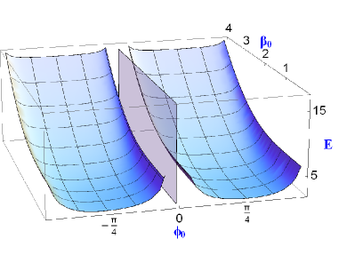
Figure 1: (Color online) Excitation energies $E_{n_{\beta},L}$ [Eq. (12)] for $n_{\beta}=0$ and $L=2$ are shown as a function of the free parameters $\beta_{0}$ and $\phi_{0}$. All quantities shown are dimensionless. See subsection II.C for further discussion.

As an example of the dependence of the energy levels on the free parameters $\beta_{0}$ and $\phi_{0}$ in Eq. (12), the energy levels with $n_{\beta}=0$ and $L=2$ are shown in Fig. 1. Smooth variation with both parameters is seen. It is worth remarking that very slight dependence on $\phi_{0}$ is observed between $\pi/8$ and $3\pi/8$, in agreement with the findings of Ref. AQOA . This observation (partly) justifies a posteriori the adiabatic approximation used in relation to the $\phi$ degree of freedom, described in Appendix D3.

II.4 $B(EL)$ transition rates

The electric quadrupole and octupole operators are (Eq. (6-63) of BM )

$$T^{(E2)}_{\mu}=t_{2}\beta_{2}{\cal D}^{(2)}_{0,\mu}(\theta)=t_{2}\sqrt{B\over B_{2}}\tilde{\beta}\cos\phi{\cal D}^{(2)}_{0,\mu}(\theta),\\ T^{(E3)}_{\mu}=t_{3}\beta_{3}{\cal D}^{(3)}_{0,\mu}(\theta)=t_{3}\sqrt{B\over B_{3}}\tilde{\beta}\sin\phi{\cal D}^{(3)}_{0,\mu}(\theta),$$ (17)

with

$$t_{2}={3Ze\over 4\pi}R^{2},\qquad t_{3}={3Ze\over 4\pi}R^{3},$$ (18)

where $R$ is the effective radius of the nucleus, while the electric dipole operator reads Dzy

$$T^{(E1)}_{\mu}=t_{1}\beta_{2}\beta_{3}{\cal D}^{(1)}_{0,\mu}(\theta)=t_{1}{B\over\sqrt{B_{2}B_{3}}}\tilde{\beta}^{2}{\sin 2\phi\over 2}{\cal D}^{(1)}_{0,\mu}(\theta).$$ (19)

The total wave function reads

$$\Phi^{\pm}_{L,M,q}(\tilde{\beta},\phi,\theta)=(\beta_{2}\beta_{3})^{-3/2}N_{\tilde{\beta}}F_{n_{\beta}}^{L}(\tilde{\beta})N_{\phi}\\ {(\chi_{n_{\phi}}(\tilde{\phi}^{+})\pm\chi_{n_{\phi}}(\tilde{\phi}^{-}))\over\sqrt{2}}\sqrt{2L+1\over 32\pi^{2}}(1\pm(-1)^{L}){\cal D}^{L}_{0,M}(\theta),$$ (20)

where $q$ stands for the rest of the quantum numbers ($n_{\beta}$, $n_{\phi}$). Since in what follows only bands with $n_{\phi}=0$ will be considered, in the remainder of the paper, as well as in the Appendices, we simplify the notation by using $n$ instead of $n_{\beta}$. As a result, in what follows, $n_{i}$ and $n_{f}$ indicate the initial and final values of $n_{\beta}$, while $q_{i}$ and $q_{f}$ denote $n_{i}$ and $n_{f}$ respectively, with $n_{\phi}=0$ at all times.

$B(EL)$ transition rates are given by

$$B(EL;L_{i}q_{i}\to L_{f}q_{f})={|\langle L_{f}q_{f}||T^{(EL)}||L_{i}q_{i}\rangle|^{2}\over(2L_{i}+1)},$$ (21)

where the reduced matrix element is obtained through the Wigner-Eckart theorem

$$\langle L_{f}\mu_{f}q_{f}|T^{(EL)}_{\mu}|L_{i}\mu_{i}q_{i}\rangle=\\ {(L_{i}LL_{f}|\mu_{i}\mu\mu_{f})\over\sqrt{2L_{f}+1}}\langle L_{f}q_{f}||T^{EL}||L_{i}q_{i}\rangle.$$ (22)

In Eq. (21) the integration over the Euler angles $\theta$ involves standard integrals over three Wigner functions calculated in Appendix B, while the rest of the integrations are performed over $\int\int\beta_{2}^{3}d\beta_{2}\beta_{3}^{3}d\beta_{3}$, where the $\beta_{2}^{3}$, $\beta_{3}^{3}$ factors come from the volume element and cancel with the first factor of Eq. (20). Using Eqs. (4) and (5), as well as the relevant Jacobian, one finds (up to constant factors) that the integration is over $\int\int d\beta_{2}d\beta_{3}={B\over\sqrt{B_{2}B_{3}}}\int\int\tilde{\beta}d\tilde{\beta}d\phi$.

Relevant integrals over $\phi$ are calculated in Appendix A, while integrals over $\tilde{\beta}$ are determined in Appendix C. The final results for matrix elements are summarized here.

Matrix elements of $T^{(E2)}$ between positive parity levels within the ground state band ($n_{i}=n_{f}=0$) read

$$\langle L_{f}q_{f}||T^{E2}||L_{i}q_{i}\rangle_{S\to S}=t_{2}\sqrt{B\over B_{2}}e^{-{1\over 4b^{2}}}{\cos\phi_{0}+e^{-b^{2}\phi_{0}^{2}}\over 1+e^{-b^{2}\phi_{0}^{2}}}\\ \sqrt{2L_{i}+1}(L_{i}2L_{f}|000)\frac{\Gamma\left(\frac{a_{i}}{2}+\frac{a_{f}}{2}+\frac{3}{2}\right)}{\sqrt{\Gamma(a_{i}+1)\Gamma(a_{f}+1)}}.$$ (23)

Matrix elements of $T^{(E2)}$ from a positive parity level of the first excited band ($n_{i}=1$) to a positive parity level of the ground state band ($n_{f}=0$) are

$$\langle L_{f}q_{f}||T^{E2}||L_{i}q_{i}\rangle_{S\to S}=t_{2}\sqrt{B\over B_{2}}\\ e^{-{1\over 4b^{2}}}{\cos\phi_{0}+e^{-b^{2}\phi_{0}^{2}}\over 1+e^{-b^{2}\phi_{0}^{2}}}\sqrt{2L_{i}+1}(L_{i}2L_{f}|000)\\ \frac{\Gamma\left(\frac{a_{i}}{2}+\frac{a_{f}}{2}+\frac{3}{2}\right)\Gamma\left(\frac{a_{i}}{2}-\frac{a_{f}}{2}+\frac{1}{2}\right)}{\sqrt{\Gamma(a_{i}+2)\Gamma(a_{f}+1)}\Gamma\left(\frac{a_{i}}{2}-\frac{a_{f}}{2}-\frac{1}{2}\right)}.$$ (24)

Matrix elements of $T^{(E2)}$ between negative parity levels within the lowest band ($n_{i}=n_{f}=0$) have the form

$$\langle L_{f}q_{f}||T^{E2}||L_{i}q_{i}\rangle_{A\to A}=t_{2}\sqrt{B\over B_{2}}e^{-{1\over 4b^{2}}}{\cos\phi_{0}-e^{-b^{2}\phi_{0}^{2}}\over 1-e^{-b^{2}\phi_{0}^{2}}}\\ \sqrt{2L_{i}+1}(L_{i}2L_{f}|000)\frac{\Gamma\left(\frac{a_{i}}{2}+\frac{a_{f}}{2}+\frac{3}{2}\right)}{\sqrt{\Gamma(a_{i}+1)\Gamma(a_{f}+1)}}.$$ (25)

Matrix elements of $T^{(E3)}$ between a positive parity level of the ground state band and a negative parity level of the lowest band, or vice versa, read

$$\langle L_{f}q_{f}||T^{E3}||L_{i}q_{i}\rangle=t_{3}\sqrt{B\over B_{3}}{e^{-{1\over 4b^{2}}}\sin\phi_{0}\over\sqrt{1-e^{-2b^{2}\phi_{0}^{2}}}}\sqrt{2L_{i}+1}\\ (L_{i}3L_{f}|000)\frac{\Gamma\left(\frac{a_{i}}{2}+\frac{a_{f}}{2}+\frac{3}{2}\right)}{\sqrt{\Gamma(a_{i}+1)\Gamma(a_{f}+1)}}.$$ (26)

Matrix elements of $T^{(E1)}$ between a positive parity level of the ground state band and a negative parity level of the lowest band, or vice versa, are

$$\langle L_{f}q_{f}||T^{E1}||L_{i}q_{i}\rangle_{S\to S}={1\over 2}t_{1}{B\over\sqrt{B_{2}B_{3}}}{e^{-{1\over b^{2}}}\sin 2\phi_{0}\over\sqrt{1-e^{-2b^{2}\phi_{0}^{2}}}}\\ \sqrt{2L_{i}+1}(L_{i}1L_{f}|000)\frac{\Gamma\left(\frac{a_{i}}{2}+\frac{a_{f}}{2}+2\right)}{\sqrt{\Gamma(a_{i}+1)\Gamma(a_{f}+1)}}.$$ (27)

The final results for $B(EL)$s are summarized here.

$B(E2)$s between positive parity levels within the ground state band ($n_{i}=n_{f}=0$) read

$$B(E2;L_{i}q_{i}\to L_{f}q_{f})_{S\to S}=t_{2}^{2}{B\over B_{2}}\\ e^{-{1\over 2b^{2}}}{(\cos\phi_{0}+e^{-b^{2}\phi_{0}^{2}})^{2}\over(1+e^{-b^{2}\phi_{0}^{2}})^{2}}\\ (L_{i}2L_{f}|000)^{2}\frac{\left[\Gamma\left(\frac{a_{i}}{2}+\frac{a_{f}}{2}+\frac{3}{2}\right)\right]^{2}}{\Gamma(a_{i}+1)\Gamma(a_{f}+1)}.$$ (28)

$B(E2)$s from a positive parity level of the first excited band ($n_{i}=1$) to a positive parity level of the ground state band ($n_{f}=0$) are

$$B(E2;L_{i}q_{i}\to L_{f}q_{f})_{S\to S}=t_{2}^{2}{B\over B_{2}}\\ e^{-{1\over 2b^{2}}}{(\cos\phi_{0}+e^{-b^{2}\phi_{0}^{2}})^{2}\over(1+e^{-b^{2}\phi_{0}^{2}})^{2}}(L_{i}2L_{f}|000)^{2}\\ \frac{\left[\Gamma\left(\frac{a_{i}}{2}+\frac{a_{f}}{2}+\frac{3}{2}\right)\Gamma\left(\frac{a_{i}}{2}-\frac{a_{f}}{2}+\frac{1}{2}\right)\right]^{2}}{\Gamma(a_{i}+2)\Gamma(a_{f}+1)\left[\Gamma\left(\frac{a_{i}}{2}-\frac{a_{f}}{2}-\frac{1}{2}\right)\right]^{2}}.$$ (29)

$B(E2)$s between negative parity levels within the lowest band ($n_{i}=n_{f}=0$) have the form

$$B(E2;L_{i}q_{i}\to L_{f}q_{f})_{A\to A}=t_{2}^{2}{B\over B_{2}}\\ e^{-{1\over 2b^{2}}}{(\cos\phi_{0}-e^{-b^{2}\phi_{0}^{2}})^{2}\over(1-e^{-b^{2}\phi_{0}^{2}})^{2}}\\ (L_{i}2L_{f}|000)^{2}\frac{\left[\Gamma\left(\frac{a_{i}}{2}+\frac{a_{f}}{2}+\frac{3}{2}\right)\right]^{2}}{\Gamma(a_{i}+1)\Gamma(a_{f}+1)}.$$ (30)

$B(E3)$s between a positive parity level of the ground state band and a negative parity level of the lowest band, or vice versa, read

$$B(E3;L_{i}q_{i}\to L_{f}q_{f})=t_{3}^{2}{B\over B_{3}}{e^{-{1\over 2b^{2}}}\sin^{2}\phi_{0}\over(1-e^{-2b^{2}\phi_{0}^{2}})}\\ (L_{i}3L_{f}|000)^{2}\frac{\left[\Gamma\left(\frac{a_{i}}{2}+\frac{a_{f}}{2}+\frac{3}{2}\right)\right]^{2}}{\Gamma(a_{i}+1)\Gamma(a_{f}+1)}.$$ (31)

$B(E1)$s between a positive parity level of the ground state band and a negative parity level of the lowest band, or vice versa, are

$$B(E1;L_{i}q_{i}\to L_{f}q_{f})={1\over 4}t_{1}^{2}{B^{2}\over B_{2}B_{3}}{e^{-{2\over b^{2}}}\sin^{2}2\phi_{0}\over(1-e^{-2b^{2}\phi_{0}^{2}})}\\ (L_{i}1L_{f}|000)^{2}\frac{\left[\Gamma\left(\frac{a_{i}}{2}+\frac{a_{f}}{2}+2\right)\right]^{2}}{\Gamma(a_{i}+1)\Gamma(a_{f}+1)}.$$ (32)

In Ref. Nomura2 it has been pointed out that $B(E1)$s for transitions from positive parity levels $L$ of the ground state band to negative parity levels $L-1$ of the lowest band and $B(E1)$s for transitions in the opposite direction, i.e. from negative parity levels $L-1$ of the lowest band to positive parity levels $L$ of the ground state band, should be of the same order, as seen experimentally. This condition is clearly fulfilled by Eq. (32).

Table 1: Parameters $\phi_{0}$ and $\beta_{0}$ of the AQOA model with Davidson potential (AQOA-D) obtained from rms fits to experimental spectra of ²²²Ra Cocks1 ; Cocks2 , ²²⁴Ra Cocks1 ; Cocks2 , ²²⁶Ra Cocks1 ; Cocks2 , ²²⁴Th Th224 , and ²²⁶Th Th226 . The experimental $R_{4/2}=E(4_{1}^{+})/E(2_{1}^{+})$ ratios are also shown. The angular momenta of the highest levels of the ground state, $\beta$ and negative parity bands included in the rms fit are labelled by $L_{g}$, $L_{\beta}$, and $L_{o}$ respectively, while $n$ indicates the total number of levels involved in the fit and $\sigma$ is the quality measure of Eq. (33). The theoretical predictions are obtained from the formulae mentioned in subsec. II.B . See subsec. III.A for further discussion. For completeness, the parameter $b$, and the parameter ratios $t_{3}/t_{2}$, and $B_{2}/B_{3}$, appearing in the fitting of electric transition rates, are shown, wherever known. All quantities shown are dimensionless, exept $t_{3}/t_{2}$, which is given in fm. See subsec. III.B for further discussion.

nucleus	$R_{4/2}$	$\phi_{0}$	$\beta_{0}$	$L_{g}$	$L_{\beta}$	$L_{o}$	$n$	$\sigma$	$b$	$t_{3}/t_{2}$(fm)	$B_{2}/B_{3}$
222Ra	2.715	62.7	0.00	20	0	19	20	0.917		7.266
224Ra	2.970	41.9	1.80	28	0	27	28	1.351	1.836	7.288	0.65
226Ra	3.127	24.7	2.14	28	0	27	28	1.360		7.309
224Th	2.896	67.9	0.79	18		17	17	0.843		7.288
226Th	3.136	9.5	0.94	20	0	19	20	0.994		7.309

Table 2: Comparison of theoretical predictions of the AQOA model with Davidson potential (AQOA-D, columns labelled as D) and with an infinite well potential (AQOA-IW, columns labelled as IW) to experimental data [normalized to $E(2_{1}^{+})$] of ²²²Ra Cocks1 ; Cocks2 , ²²⁴Ra Cocks1 ; Cocks2 , ²²⁶Ra Cocks1 ; Cocks2 , ²²⁴Th Th224 , and ²²⁶Th Th226 . The AQOA-D parameters are shown in Table I, while the AQOA-IW predictions have been taken from Ref. AQOA . The theoretical predictions for AQOA-D are obtained from the formulae mentioned in subsec. II.B . See subsec. III.A for further discussion.

	222Ra	222Ra	224Ra	224Ra	226Ra	226Ra	226Ra	224Th	224Th	226Th	226Th	226Th
$L^{\pi}$	exp.	D	exp.	D	exp.	D	IW	exp.	D	exp.	D	IW
$4^{+}$	2.72	3.00	2.97	3.17	3.13	3.22	3.09	2.90	3.09	3.14	3.22	3.12
$6^{+}$	4.95	5.59	5.68	6.21	6.16	6.45	5.99	5.45	5.90	6.20	6.44	6.10
$8^{+}$	7.58	8.49	8.94	9.87	9.89	10.45	9.56	8.50	9.17	10.00	10.42	9.78
$10^{+}$	10.55	11.58	12.66	13.94	14.19	15.02	13.71	11.97	12.71	14.41	14.97	14.08
$12^{+}$	13.82	14.77	16.74	18.30	18.93	20.00	18.42	15.80	16.42	19.32	19.93	18.96
$14^{+}$	17.39	18.04	21.17	22.85	24.06	25.31	23.64	19.97	20.25	24.68	25.20	24.38
$16^{+}$	21.21	21.36	25.90	27.55	29.52	30.84	29.38	24.44	24.16	30.41	30.69	30.34
$18^{+}$	25.28	24.70	30.92	32.34	35.30	36.54	35.61	29.20	28.13	36.50	36.35	36.81
$20^{+}$	29.57	28.07	36.22	37.22	41.38	42.38	42.33			42.90	42.14	43.80
$22^{+}$			41.74	42.15	47.75	48.32	49.54
$24^{+}$			47.48	47.13	54.44	54.34	57.22
$26^{+}$			53.41	52.14	61.42	60.43	65.38
$28^{+}$			59.54	57.18	68.70	66.57	74.01
$0^{+}$	8.23	8.06	10.86	10.90	12.19	12.21	11.23		9.91	11.18	11.31	12.41
$1^{-}$	2.18	0.35	2.56	0.34	3.75	0.34	0.34	2.56	0.34	3.19	0.34	0.34
$3^{-}$	2.85	1.90	3.44	1.95	4.75	1.97	1.93	3.11	1.93	4.26	1.97	1.94
$5^{-}$	4.26	4.24	5.13	4.60	6.60	4.72	4.45	4.74	4.43	6.24	4.72	4.51
$7^{-}$	6.33	7.01	7.59	7.98	9.26	8.36	7.70	7.13	7.49	9.11	8.35	7.86
$9^{-}$	8.92	10.02	10.73	11.86	12.68	12.67	11.57	10.17	10.91	12.79	12.64	11.86
$11^{-}$	11.97	13.17	14.46	16.09	16.74	17.47	16.00	13.73	14.55	17.15	17.41	16.45
$13^{-}$	15.38	16.40	18.68	20.56	21.39	22.63	20.96	17.72	18.32	22.11	22.53	21.61
$15^{-}$	19.11	19.69	23.31	25.18	26.54	28.05	26.45	22.07	22.20	27.55	27.92	27.30
$17^{-}$	23.11	23.03	28.27	29.93	32.13	33.67	32.43	26.71	26.14	33.42	33.50	33.51
$19^{-}$	27.35	26.39	33.51	34.77	38.10	39.44	38.91			39.63	39.23	40.24
$21^{-}$			38.99	39.68	44.41	45.34	45.87
$23^{-}$			44.67	44.63	51.03	51.32	53.32
$25^{-}$			50.55	49.63	57.93	57.38	61.24
$27^{-}$			56.60	54.66	65.08	63.49	69.64

III Numerical results

III.1 Spectra

In the spectra of the AQOA model with Davidson potential (AQOA-D) only the parameters $\phi_{0}$ and $\beta_{0}$ play an essential role, as seen in Eq. (12), while the quantities $E_{0}$, $C_{1}$, and $C_{2}$ of Eq. (16) do not enter, if we consider only bands with $n_{\phi}=0$ and normalize all energies to that of the first excited state, $E(2^{+}_{1})$. The parameters of rms fits, using the quality measure

$$\sigma=\sqrt{{\sum_{i=1}^{n}(E_{i}(exp)-E_{i}(th))^{2}\over(n-1)E(2_{1}^{+})^{2}}},$$ (33)

to the spectra of the Ra and Th isotopes lying at the border between the regions of octupole deformation and octupole vibrations, as well as within the former region, are shown in Table I, while in Table II the relevant spectra are shown. For ²²⁶Ra and ²²⁶Th, the predictions of the original one-parameter ($\phi_{0}$) AQOA with an infinite well potential (AQOA-IW), applicable at the border between the regions of octupole deformation and octupole vibrations, are shown for comparison. The following comments apply.

a) Good agreement between the theoretical predictions of AQOA-D and experimental data is obtained up to high angular momenta, both in the ground state band and in the negative parity band. The predictions for the $1^{-}$ and $3^{-}$ states are poor, since no finite barrier is used in the phi potential Jolos49 ; Jolos587 ; Jolos60

b) When moving from the border region towards the interior of the region of octupole deformation, the parameter $\phi_{0}$ increases, in agreement with an increasing role of the octupole deformation (which is proportional to $\sin\phi_{0}$), while the parameter $\beta_{0}$ decreases. In parallel, a decreasing role of the quadrupole deformation is revealed by the decreasing $R_{4/2}$ ratios.

c) The agreement between the predictions of AQOA-IW and the data is comparable to that of AQOA-D, except at high angular momenta, where AQOA-D is closer to the data, due to the term $\beta_{0}^{4}$ appearing in Eq. (12), which moderates the increase of the energy with $L$.

III.2 Transitions

With the parameters $\phi_{0}$ and $\beta_{0}$ determined from the spectra, we now turn attention to electromagnetic transition rates, following the procedure described below.

a) From Eqs. (28) and (29) it is clear that ratios of $B(E2)_{S\to S}$s involve only the parameters $\phi_{0}$ and $\beta_{0}$, thus they are already fixed. The same holds separately for ratios of $B(E2)_{A\to A}$s, or $B(E3)$s, or $B(E1)$s, as seen from Eqs. (30), (31), and (32) respectively.

b) Ratios of $B(E2)_{S\to S}$s over $B(E2)_{A\to A}$s involve in addition the parameter $b$, which can then be determined from such ratios, as seen from Eqs. (28) and (30).

c) Ratios of $B(E3)$s over $B(E2)$s involve in addition the ratio $t_{3}/t_{2}$, which can be determined from the nuclear radius (see subsec. III.B.2), and the ratio $B_{2}/B_{3}$, which can be determined from the $B(E3)/B(E2)$ ratios, as seen from Eqs. (31) and (28).

This procedure can be tested against the recently measured transition matrix elements of ²²⁴Ra 224Ra , shown in Table III.

Table 3: Matrix elements of electric transitions in ²²⁴Ra. The experimental data, in units of $e$ fm, $e$ fm², $e$ fm³ for E1, E2, E3 respectively, have been taken from Ref. 224Ra , while the theoretical predictions have been obtained using the formulae of subsec. II.D in the way described in subsec. III.B, where further discussion is given.

m.e.	exp.	th.
$\langle 0^{+}||E2||2^{+}\rangle$	199$\pm$3	196
$\langle 2^{+}||E2||4^{+}\rangle$	315$\pm$6	323
$\langle 4^{+}||E2||6^{+}\rangle$	405$\pm$15	426
$\langle 6^{+}||E2||8^{+}\rangle$	500$\pm$60	525
$\langle 1^{-}||E2||3^{-}\rangle$	230$\pm$11	236
$\langle 3^{-}||E2||5^{-}\rangle$	410$\pm$60	334
$\langle 0^{+}||E2||2^{+}_{\gamma}\rangle$	23$\pm$4	36
$\langle 0^{+}||E3||3^{-}\rangle$	940$\pm$30	1006
$\langle 2^{+}||E3||1^{-}\rangle$	1370$\pm$140	1137
$\langle 2^{+}||E3||3^{-}\rangle$	$<$4000	1176
$\langle 2^{+}||E3||5^{-}\rangle$	1410$\pm$190	1594
$\langle 0^{+}||E1||1^{-}\rangle$	$<$0.018	0.013
$\langle 2^{+}||E1||1^{-}\rangle$	$<$0.03	0.018
$\langle 2^{+}||E1||3^{-}\rangle$	0.026$\pm$0.005	0.023
$\langle 4^{+}||E1||5^{-}\rangle$	0.030$\pm$0.010	0.032
$\langle 6^{+}||E1||7^{-}\rangle$	$<$0.10	0.042

III.2.1 $E2$ transitions

The ratio of any $E2_{A\to A}$ matrix element [Eq. (25)] over any $E2_{S\to S}$ matrix element [Eq. (23)] contains the ratio

$$r={(\cos\phi_{0}-a)(1+a)\over(\cos\phi_{0}+a)(1-a)},\qquad a=e^{-b^{2}\phi_{0}^{2}}.$$ (34)

In the case of ²²⁴Ra, the ratios of experimental matrix elements ${3^{-}\to 1^{-}\over 2^{+}\to 0^{+}}$, ${3^{-}\to 1^{-}\over 4^{+}\to 2^{+}}$, ${3^{-}\to 1^{-}\over 6^{+}\to 4^{+}}$, ${3^{-}\to 1^{-}\over 8^{+}\to 6^{+}}$ lead to $r=0.852$, 0.887, 0.909, 0.908, i.e., to an average value of 0.889 .

Solving for $a$ one obtains the quadratic equation

$$(r-1)a^{2}+(r+1)(\cos\phi_{0}-1)a+(1-r)\cos\phi_{0}=0,$$ (35)

having the solution

$$a={1\over 2(r-1)}\left[-(r+1)(\cos\phi_{0}-1)\right.\\ \left.\pm\sqrt{(r+1)^{2}(\cos\phi_{0}-1)^{2}+4(r-1)^{2}\cos\phi_{0}}\right].$$ (36)

Since from Eq. (34) one has

$$b^{2}=-{\ln a\over\phi_{0}^{2}},$$ (37)

$\ln a$ has to be negative for $b$ to be real. Since $r<1$, we see that in Eq. (36) only the negative sign is allowed in order to have $a>0$, leading in the case of ²²⁴Ra to $a=0.1647$ and $b=1.836$ .

One can then keep

$$F=t_{2}\sqrt{B/B_{2}}$$ (38)

as an overall constant for all $E2$ transition matrix elements, and determine it through rms fitting to the experimental data of the transitions with $n_{i}=n_{f}=0$, obtaining $F=127.20$ and the $E2$ predictions reported in Table III. Then from Eq. (24) one can calculate also the transitions with $n_{i}=1$, $n_{f}=0$, one of which is also reported in Table III.

III.2.2 $E3$ transitions

For the coefficients $t_{2}$ and $t_{3}$ one can use Eq. (18), leading to

$${t_{3}\over t_{2}}=R,$$ (39)

where $R$ is the nuclear radius, given by Heyde

$$R=r_{0}A^{1/3},\qquad r_{0}=1.2\ {\rm fm},$$ (40)

with $A$ being the mass number of the nucleus. Thus in the case of ²²⁴Ra one has $R=7.2878$ fm.

One can then determine the ratio $B_{2}\over B_{3}$ from any ratio of $E3$ matrix element over $E2$ matrix element, since each of these ratios contains the quantity $(t_{3}/t_{2})\sqrt{B_{2}/B_{3}}$, as seen from Eqs. (26), (23), (25). In the case of ²²⁴Ra, six $E2$ matrix elements and three $E3$ matrix elements are known. Considering all 18 possible ratios, we get an average value of $(t_{3}/t_{2})\sqrt{B_{2}/B_{3}}=5.876$, leading to $B_{2}/B_{3}=0.65$.

By now the $E3$ transition matrix elements have been completely determined. The overall constant

$$F^{\prime}=t_{3}\sqrt{B/B_{3}}$$ (41)

appearing in this case is connected to the overall constant $F$ through

$${F^{\prime}\over F}={t_{3}\over t_{2}}\sqrt{B_{2}\over B_{3}}=R\sqrt{B_{2}\over B_{3}},$$ (42)

leading to $F^{\prime}=747.47$ and to the $E3$ matrix elements given in Table III.

III.2.3 $E1$ transitions

In the case of $E1$ matrix elements, the quantity

$$F^{\prime\prime}={1\over 2}t_{1}{B\over\sqrt{B_{2}B_{3}}}{e^{-{1\over b^{2}}}\sin 2\phi_{0}\over\sqrt{1-e^{-2b^{2}\phi_{0}^{2}}}}$$ (43)

can be treated as an overall constant, determined in the case of ²²⁴Ra by rms fitting to the two known transitions to be $F^{\prime\prime}=2.676\ 10^{-3}$ and providing the predictions given in Table III.

IV Conclusions

The analytic quadrupole octupole axially symmetric model with an infinite well potential (AQOA-IW) had successfully predicted the border between the regions of octupole deformation and octupole vibrations in the light actinides, identifying ²²⁶Ra and ²²⁶Th as border nuclei AQOA , with heavier isotopes corresponding to octupole vibrations and lighter isotopes exhibiting octupole deformation. The AQOA-IW model involved only one free parameter, $\phi_{0}$, expressing the relative presence of quadrupole vs. octupole deformation, while a parameter-free version has also been developed later Lenis .

In the present work, the infinite well potential is substituted by a Davidson potential, resulting in the AQOA-D model, which is able to deviate from the border line into the region of octupole deformation. This is achieved through the extra parameter $\beta_{0}$, the position of the minimum of the Davidson potential, which is increasing with increasing $R_{4/2}$ ratios, as it is known from its use in the description of quadrupole deformed nuclei ESD .

Within the AQOA-D model, analytic expressions for energy spectra and B(E1), B(E2), B(E3) transition rates are derived. Then the following path is taken.

a) The spectra of ^222-226Ra and ^224,226Th [normalized to $E(2_{1}^{+})$] are well reproduced in terms of the above mentioned two parameters $\phi_{0}$ and $\beta_{0}$.

b) The parameter $b$, related to the harmonic oscillator potential used in the $\phi$ degree of freedom, can be determined from the ratio of any $E2$ matrix element between negative parity states over any $E2$ matrix element between positive parity states, fixing the determination of all $E2$ transitions up to an overall scale factor.

c) The ratio of mass parameters $B_{2}/B_{3}$ can be determined from the ratio of any $E3$ matrix element over any $E2$ matrix element, while the ratio of transition coefficients $t_{2}/t_{3}$ is fixed by the nuclear radius. As a result, the determination of all $E2$ and $E3$ transitions is fixed, without any additional overall scale factor.

d) $E1$ transitions are also fixed, up to another scale factor.

The recently measured $B(EL)$ transition rates of ²²⁴Ra 224Ra , presenting stable octupole deformation, provide a successful test for the model. It is clear that for other nuclei, the minimum set of data needed includes

a) A few energy levels of both positive and negative parity, from which the parameters $\phi_{0}$ and $\beta_{0}$ can be determined.

b) At least one $E2$ transition between positive parity states and one $E2$ transition between negative parity states, from which the parameter $b$ can be determined.

c) At least one $E3$ transition, from which, in combination with the $E2$ transitions of b), the parameter ratio $B_{2}/B_{3}$ can be determined.

From these pieces of data

a) The spectrum (leaving out the $\gamma$ bands) is determined up to an overall scale factor.

b) All relevant $E2$ and $E3$ transitions are determined up to an overall scale factor.

c) All relevant $E1$ transitions are determined up to another overall scale factor.

It is of interest to apply the present model in the actinides close to ²⁴⁰Pu, in which a second order shape phase transition from octupole-nondeformed to octupole-deformed shapes has been recently found Jolos86 , while octupole bands have been described Jolos88 using supersymmetric quantum mechanics. The light rare earths, in which octupole bands have been considered recently both by the Bizzeti and Bizzeti-Sona approach Bizzeti81 and within density functional theory Guzman , are also of special interest. A successful application of the AQOA-IW model to ¹⁴⁸Nd has already been given in Ref. Sugawara .

Appendix A. $\phi$ integrals

Since we confine ourselves to states with $n_{\phi}=0$, this quantum number is omitted in the notation of the wave functions, which then carry only the subscript $i$ ($f$) for the initial (final) state.

For symmetric states one has

$$X_{S}(\phi)=N_{S}{\chi(\tilde{\phi}^{+})+\chi(\tilde{\phi}^{-})\over\sqrt{2}},$$ (44)

while for antisymmetric states one has

$$X_{A}(\phi)=N_{A}{\chi(\tilde{\phi}^{+})-\chi(\tilde{\phi}^{-})\over\sqrt{2}},$$ (45)

where $N_{S}$ and $N_{A}$ are normalization factors and, according to Eq. (15),

$$\chi(\tilde{\phi}^{+})=\sqrt{b\over\sqrt{\pi}}e^{-{b^{2}\over 2}(\phi-\phi_{0})^{2}},\\ \chi(\tilde{\phi}^{-})=\sqrt{b\over\sqrt{\pi}}e^{-{b^{2}\over 2}(\phi+\phi_{0})^{2}}.$$ (46)

A0. Normalization

For symmetric states one has

$${1\over N_{S}^{2}}=\int_{-\infty}^{\infty}X_{S}X_{S}d\phi\\ ={1\over 2}\int_{-\infty}^{\infty}(\chi(\phi^{+}))^{2}d\phi+{1\over 2}\int_{-\infty}^{\infty}(\chi(\phi^{-}))^{2}d\phi\\ +\int_{-\infty}^{\infty}\chi(\phi^{+})\chi(\phi^{-})d\phi\\ ={1\over 2}{b\over\sqrt{\pi}}e^{-b^{2}\phi_{0}^{2}}\int_{-\infty}^{\infty}e^{-b^{2}\phi^{2}+2b^{2}\phi_{0}\phi}d\phi\\ +{1\over 2}{b\over\sqrt{\pi}}e^{-b^{2}\phi_{0}^{2}}\int_{-\infty}^{\infty}e^{-b^{2}\phi^{2}-2b^{2}\phi_{0}\phi}d\phi\\ +{b\over\sqrt{\pi}}e^{-b^{2}\phi_{0}^{2}}\int_{-\infty}^{\infty}e^{-b^{2}\phi^{2}}d\phi.$$ (47)

Using Eq. (84) of Appendix A4 we see that the integrals appearing here are of the form

$$\int_{-\infty}^{\infty}e^{-b^{2}\phi^{2}\pm 2b^{2}\phi_{0}\phi}d\phi={\sqrt{\pi}\over b}e^{b^{2}\phi_{0}^{2}},$$ (48)

leading to

$${1\over N_{S}^{2}}=1+e^{-b^{2}\phi_{0}^{2}}.$$ (49)

For antisymmetric states one has

$${1\over N_{A}^{2}}=\int_{-\infty}^{\infty}X_{A}X_{A}d\phi\\ ={1\over 2}\int_{-\infty}^{\infty}(\chi(\phi^{+}))^{2}d\phi+{1\over 2}\int_{-\infty}^{\infty}(\chi(\phi^{-}))^{2}d\phi\\ -\int_{-\infty}^{\infty}\chi(\phi^{+})\chi(\phi^{-})d\phi\\ ={1\over 2}{b\over\sqrt{\pi}}e^{-b^{2}\phi_{0}^{2}}\int_{-\infty}^{\infty}e^{-b^{2}\phi^{2}+2b^{2}\phi_{0}\phi}d\phi\\ +{1\over 2}{b\over\sqrt{\pi}}e^{-b^{2}\phi_{0}^{2}}\int_{-\infty}^{\infty}e^{-b^{2}\phi^{2}-2b^{2}\phi_{0}\phi}d\phi\\ -{b\over\sqrt{\pi}}e^{-b^{2}\phi_{0}^{2}}\int_{-\infty}^{\infty}e^{-b^{2}\phi^{2}}d\phi,$$ (50)

leading in the same way as above to

$${1\over N_{A}^{2}}=1-e^{-b^{2}\phi_{0}^{2}}.$$ (51)

A1. $B(E2)$s

The transition operator for $B(E2)$s contains $\tilde{\beta}_{2}=\tilde{\beta}\cos\phi$.

For $B(E2)$s between symmetric states one has

$$I_{\phi,S\to S}^{(E2)}=\int_{-\infty}^{\infty}X_{S}\cos\phi X_{S}d\phi\\ ={N_{S}^{2}\over 2}\int_{-\infty}^{\infty}(\chi(\phi^{+}))^{2}\cos\phi d\phi\\ +{N_{S}^{2}\over 2}\int_{-\infty}^{\infty}(\chi(\phi^{-}))^{2}\cos\phi d\phi\\ +N_{S}^{2}\int_{-\infty}^{\infty}\chi(\phi^{+})\chi(\phi^{-})\cos\phi d\phi\\ ={N_{S}^{2}\over 2}{b\over\sqrt{\pi}}e^{-b^{2}\phi_{0}^{2}}\int_{-\infty}^{\infty}e^{-b^{2}\phi^{2}+2b^{2}\phi_{0}\phi}\cos\phi d\phi\\ +{N_{S}^{2}\over 2}{b\over\sqrt{\pi}}e^{-b^{2}\phi_{0}^{2}}\int_{-\infty}^{\infty}e^{-b^{2}\phi^{2}-2b^{2}\phi_{0}\phi}\cos\phi d\phi\\ +N_{S}^{2}{b\over\sqrt{\pi}}e^{-b^{2}\phi_{0}^{2}}\int_{-\infty}^{\infty}e^{-b^{2}\phi^{2}}\cos\phi d\phi.$$ (52)

Using Eq. (81) of Appendix A4 we see that the integrals appearing here are of the form

$$\int_{-\infty}^{\infty}e^{-b^{2}\phi^{2}\pm 2b^{2}\phi_{0}\phi}\cos\phi d\phi={\sqrt{\pi}\over b}e^{b^{2}\phi_{0}^{2}-{1\over 4b^{2}}}\cos\phi_{0},$$ (53)

leading to

$$I_{\phi,S\to S}^{(E2)}=e^{-{1\over 4b^{2}}}{\cos\phi_{0}+e^{-b^{2}\phi_{0}^{2}}\over 1+e^{-b^{2}\phi_{0}^{2}}}.$$ (54)

For $B(E2)$s between antisymmetric states one has

$$I_{\phi,A\to A}^{(E2)}=\int_{-\infty}^{\infty}X_{A}\cos\phi X_{A}d\phi\\ ={N_{A}^{2}\over 2}\int_{-\infty}^{\infty}(\chi(\phi^{+}))^{2}\cos\phi d\phi\\ +{N_{A}^{2}\over 2}\int_{-\infty}^{\infty}(\chi(\phi^{-}))^{2}\cos\phi d\phi\\ -N_{A}^{2}\int_{-\infty}^{\infty}\chi(\phi^{+})\chi(\phi^{-})\cos\phi d\phi\\ ={N_{A}^{2}\over 2}{b\over\sqrt{\pi}}e^{-b^{2}\phi_{0}^{2}}\int_{-\infty}^{\infty}e^{-b^{2}\phi^{2}+2b^{2}\phi_{0}\phi}\cos\phi d\phi\\ +{N_{A}^{2}\over 2}{b\over\sqrt{\pi}}e^{-b^{2}\phi_{0}^{2}}\int_{-\infty}^{\infty}e^{-b^{2}\phi^{2}-2b^{2}\phi_{0}\phi}\cos\phi d\phi\\ -N_{A}^{2}{b\over\sqrt{\pi}}e^{-b^{2}\phi_{0}^{2}}\int_{-\infty}^{\infty}e^{-b^{2}\phi^{2}}\cos\phi d\phi,$$ (55)

leading in the same way as above to

$$I_{\phi,A\to A}^{(E2)}=e^{-{1\over 4b^{2}}}{\cos\phi_{0}-e^{-b^{2}\phi_{0}^{2}}\over 1-e^{-b^{2}\phi_{0}^{2}}}.$$ (56)

For $B(E2)$s between symmetric and antisymmetric states one has

$$I_{\phi,S\to A}^{(E2)}=\int_{-\infty}^{\infty}X_{S}\cos\phi X_{A}d\phi\\ ={N_{S}N_{A}\over 2}\int_{-\infty}^{\infty}(\chi(\phi^{+}))^{2}\cos\phi d\phi\\ -{N_{S}N_{A}\over 2}\int_{-\infty}^{\infty}(\chi(\phi^{-}))^{2}\cos\phi d\phi\\ ={N_{S}N_{A}\over 2}{b\over\sqrt{\pi}}e^{-b^{2}\phi_{0}^{2}}\int_{-\infty}^{\infty}e^{-b^{2}\phi^{2}+2b^{2}\phi_{0}\phi}\cos\phi d\phi\\ -{N_{S}N_{A}\over 2}{b\over\sqrt{\pi}}e^{-b^{2}\phi_{0}^{2}}\int_{-\infty}^{\infty}e^{-b^{2}\phi^{2}-2b^{2}\phi_{0}\phi}\cos\phi d\phi,$$ (57)

leading to

$$I_{\phi,S\to A}^{(E2)}=0.$$ (58)

In the same way one also finds

$$I_{\phi,A\to S}^{(E2)}=0.$$ (59)

A2. $B(E3)$s

The transition operator for $B(E3)$s contains $\tilde{\beta}_{3}=\tilde{\beta}\sin\phi$.

For $B(E3)$s between symmetric states one has

$$I_{\phi,S\to S}^{(E3)}=\int_{-\infty}^{\infty}X_{S}\sin\phi X_{S}d\phi\\ ={N_{S}^{2}\over 2}\int_{-\infty}^{\infty}(\chi(\phi^{+}))^{2}\sin\phi d\phi\\ +{N_{S}^{2}\over 2}\int_{-\infty}^{\infty}(\chi(\phi^{-}))^{2}\sin\phi d\phi\\ +N_{S}^{2}\int_{-\infty}^{\infty}\chi(\phi^{+})\chi(\phi^{-})\sin\phi d\phi\\ ={N_{S}^{2}\over 2}{b\over\sqrt{\pi}}e^{-b^{2}\phi_{0}^{2}}\int_{-\infty}^{\infty}e^{-b^{2}\phi^{2}+2b^{2}\phi_{0}\phi}\sin\phi d\phi\\ +{N_{S}^{2}\over 2}{b\over\sqrt{\pi}}e^{-b^{2}\phi_{0}^{2}}\int_{-\infty}^{\infty}e^{-b^{2}\phi^{2}-2b^{2}\phi_{0}\phi}\sin\phi d\phi\\ +N_{S}^{2}{b\over\sqrt{\pi}}e^{-b^{2}\phi_{0}^{2}}\int_{-\infty}^{\infty}e^{-b^{2}\phi^{2}}\sin\phi d\phi.$$ (60)

Using Eq. (83) of Appendix A4 we see that the integrals appearing here are of the form

$$\int_{-\infty}^{\infty}e^{-b^{2}\phi^{2}\pm 2b^{2}\phi_{0}\phi}\sin\phi d\phi=\pm{\sqrt{\pi}\over b}e^{b^{2}\phi_{0}^{2}-{1\over 4b^{2}}}\sin\phi_{0},$$ (61)

leading to

$$I_{\phi,S\to S}^{(E3)}=0.$$ (62)

For $B(E3)$s between antisymmetric states one has

$$I_{\phi,A\to A}^{(E3)}=\int_{-\infty}^{\infty}X_{A}\sin\phi X_{A}d\phi\\ ={N_{S}^{2}\over 2}\int_{-\infty}^{\infty}(\chi(\phi^{+}))^{2}\sin\phi d\phi\\ +{N_{S}^{2}\over 2}\int_{-\infty}^{\infty}(\chi(\phi^{-}))^{2}\sin\phi d\phi\\ -N_{S}^{2}\int_{-\infty}^{\infty}\chi(\phi^{+})\chi(\phi^{-})\sin\phi d\phi\\ ={N_{S}^{2}\over 2}{b\over\sqrt{\pi}}e^{-b^{2}\phi_{0}^{2}}\int_{-\infty}^{\infty}e^{-b^{2}\phi^{2}+2b^{2}\phi_{0}\phi}\sin\phi d\phi\\ +{N_{S}^{2}\over 2}{b\over\sqrt{\pi}}e^{-b^{2}\phi_{0}^{2}}\int_{-\infty}^{\infty}e^{-b^{2}\phi^{2}-2b^{2}\phi_{0}\phi}\sin\phi d\phi\\ -N_{S}^{2}{b\over\sqrt{\pi}}e^{-b^{2}\phi_{0}^{2}}\int_{-\infty}^{\infty}e^{-b^{2}\phi^{2}}\sin\phi d\phi,$$ (63)

leading in the same way as above to

$$I_{\phi,A\to A}^{(E3)}=0.$$ (64)

For $B(E3)$s between symmetric and antisymmetric states one has

$$I_{\phi,S\to A}^{(E3)}=\int_{-\infty}^{\infty}X_{S}\sin\phi X_{A}d\phi\\ ={N_{S}N_{A}\over 2}\int_{-\infty}^{\infty}(\chi(\phi^{+}))^{2}\sin\phi d\phi\\ -{N_{S}N_{A}\over 2}\int_{-\infty}^{\infty}(\chi(\phi^{-}))^{2}\sin\phi d\phi\\ ={N_{S}N_{A}\over 2}{b\over\sqrt{\pi}}e^{-b^{2}\phi_{0}^{2}}\int_{-\infty}^{\infty}e^{-b^{2}\phi^{2}+2b^{2}\phi_{0}\phi}\sin\phi d\phi\\ -{N_{S}N_{A}\over 2}{b\over\sqrt{\pi}}e^{-b^{2}\phi_{0}^{2}}\int_{-\infty}^{\infty}e^{-b^{2}\phi^{2}-2b^{2}\phi_{0}\phi}\sin\phi d\phi,$$ (65)

leading to

$$I_{\phi,S\to A}^{(E3)}={e^{-{1\over 4b^{2}}}\sin\phi_{0}\over\sqrt{1-e^{-2b^{2}\phi_{0}^{2}}}}.$$ (66)

In the same way one finds

$$I_{\phi,A\to S}^{(E3)}=I_{\phi,S\to A}^{(E3)}.$$ (67)

A3. $B(E1)$s

The transition operator for $B(E1)$s contains $\tilde{\beta}_{2}\tilde{\beta}_{3}=\tilde{\beta}\cos\phi\tilde{\beta}\sin\phi=\tilde{\beta}^{2}{\sin 2\phi\over 2}$.

For $B(E1)$s between symmetric states one has

$$I_{\phi,S\to S}^{(E1)}={1\over 2}\int_{-\infty}^{\infty}X_{S}\sin 2\phi X_{S}d\phi\\ ={N_{S}^{2}\over 4}\int_{-\infty}^{\infty}(\chi(\phi^{+}))^{2}\sin 2\phi d\phi\\ +{N_{S}^{2}\over 4}\int_{-\infty}^{\infty}(\chi(\phi^{-}))^{2}\sin 2\phi d\phi\\ +{N_{S}^{2}\over 2}\int_{-\infty}^{\infty}\chi(\phi^{+})\chi(\phi^{-})\sin 2\phi d\phi\\ ={N_{S}^{2}\over 4}{b\over\sqrt{\pi}}e^{-b^{2}\phi_{0}^{2}}\int_{-\infty}^{\infty}e^{-b^{2}\phi^{2}+2b^{2}\phi_{0}\phi}\sin 2\phi d\phi\\ +{N_{S}^{2}\over 4}{b\over\sqrt{\pi}}e^{-b^{2}\phi_{0}^{2}}\int_{-\infty}^{\infty}e^{-b^{2}\phi^{2}-2b^{2}\phi_{0}\phi}\sin 2\phi d\phi\\ +{N_{S}^{2}\over 2}{b\over\sqrt{\pi}}e^{-b^{2}\phi_{0}^{2}}\int_{-\infty}^{\infty}e^{-b^{2}\phi^{2}}\sin 2\phi d\phi.$$ (68)

Using Eq. (83) of Appendix A4 we see that the integrals appearing here are of the form

$$\int_{-\infty}^{\infty}e^{-b^{2}\phi^{2}\pm 2b^{2}\phi_{0}\phi}\sin 2\phi d\phi=\pm{\sqrt{\pi}\over b}e^{b^{2}\phi_{0}^{2}-{1\over b^{2}}}\sin 2\phi_{0},$$ (69)

leading to

$$I_{\phi,S\to S}^{(E1)}=0.$$ (70)

For $B(E1)$s between antisymmetric states one has

$$I_{\phi,A\to A}^{(E1)}={1\over 2}\int_{-\infty}^{\infty}X_{A}\sin 2\phi X_{A}d\phi\\ ={N_{A}^{2}\over 4}\int_{-\infty}^{\infty}(\chi(\phi^{+}))^{2}\sin 2\phi d\phi\\ +{N_{A}^{2}\over 4}\int_{-\infty}^{\infty}(\chi(\phi^{-}))^{2}\sin 2\phi d\phi\\ -{N_{A}^{2}\over 2}\int_{-\infty}^{\infty}\chi(\phi^{+})\chi(\phi^{-})\sin 2\phi d\phi\\ ={N_{A}^{2}\over 4}{b\over\sqrt{\pi}}e^{-b^{2}\phi_{0}^{2}}\int_{-\infty}^{\infty}e^{-b^{2}\phi^{2}+2b^{2}\phi_{0}\phi}\sin 2\phi d\phi\\ +{N_{A}^{2}\over 4}{b\over\sqrt{\pi}}e^{-b^{2}\phi_{0}^{2}}\int_{-\infty}^{\infty}e^{-b^{2}\phi^{2}-2b^{2}\phi_{0}\phi}\sin 2\phi d\phi\\ -{N_{A}^{2}\over 2}{b\over\sqrt{\pi}}e^{-b^{2}\phi_{0}^{2}}\int_{-\infty}^{\infty}e^{-b^{2}\phi^{2}}\sin 2\phi d\phi,$$ (71)

leading in the same way as above to

$$I_{\phi,A\to A}^{(E1)}=0.$$ (72)

For $B(E1)$s between symmetric and antisymmetric states one has

$$I_{\phi,S\to A}^{(E1)}={1\over 2}\int_{-\infty}^{\infty}X_{S}\sin 2\phi X_{A}d\phi\\ ={N_{S}N_{A}\over 4}\int_{-\infty}^{\infty}(\chi(\phi^{+}))^{2}\sin 2\phi d\phi\\ -{N_{S}N_{A}\over 4}\int_{-\infty}^{\infty}(\chi(\phi^{-}))^{2}\sin 2\phi d\phi\\ ={N_{S}N_{A}\over 4}{b\over\sqrt{\pi}}e^{-b^{2}\phi_{0}^{2}}\int_{-\infty}^{\infty}e^{-b^{2}\phi^{2}+2b^{2}\phi_{0}\phi}\sin 2\phi d\phi\\ -{N_{S}N_{A}\over 4}{b\over\sqrt{\pi}}e^{-b^{2}\phi_{0}^{2}}\int_{-\infty}^{\infty}e^{-b^{2}\phi^{2}-2b^{2}\phi_{0}\phi}\sin 2\phi d\phi,$$ (73)

leading to

$$I_{\phi,S\to A}^{(E1)}={e^{-{1\over b^{2}}}\sin 2\phi_{0}\over 2\sqrt{1-e^{-2b^{2}\phi_{0}^{2}}}}.$$ (74)

In the same way one finds

$$I_{\phi,A\to S}^{(E1)}=I_{\phi,S\to A}^{(E1)}.$$ (75)

A4. Useful integrals

We know that (Eq. 3.897.2 of Ref. Grad )

$$\int_{0}^{\infty}e^{-\beta x^{2}-\gamma x}\cos bxdx=\\ {1\over 4}\sqrt{\pi\over b}\left\{e^{(\gamma-ib)^{2}/(4\beta)}\left[1-\Phi\left(\gamma-ib\over 2\sqrt{\beta}\right)\right]\right.\\ \left.+e^{(\gamma+ib)^{2}/(4\beta)}\left[1-\Phi\left(\gamma+ib\over 2\sqrt{\beta}\right)\right]\right\},$$ (76)

where $Re\beta>0$, $\quad b>0$, and $\Phi(x)$ is the error function, having the property

$$\Phi(-x)=-\Phi(x).$$ (77)

Changing the variable into $y=-x$, Eq. (76) takes the form

$$-\int_{0}^{-\infty}e^{-\beta y^{2}+\gamma y}\cos bydy=\\ {1\over 4}\sqrt{\pi\over b}\left\{e^{(\gamma-ib)^{2}/(4\beta)}\left[1-\Phi\left(\gamma-ib\over 2\sqrt{\beta}\right)\right]\right.\\ \left.+e^{(\gamma+ib)^{2}/(4\beta)}\left[1-\Phi\left(\gamma+ib\over 2\sqrt{\beta}\right)\right]\right\},$$ (78)

Changing the symbol $y$ into $x$ and letting $\gamma\to-\gamma$, one then gets

$$\int_{-\infty}^{0}e^{-\beta x^{2}-\gamma x}\cos bxdx=\\ {1\over 4}\sqrt{\pi\over b}\left\{e^{(-\gamma-ib)^{2}/(4\beta)}\left[1-\Phi\left(-\gamma-ib\over 2\sqrt{\beta}\right)\right]\right.\\ \left.+e^{(-\gamma+ib)^{2}/(4\beta)}\left[1-\Phi\left(-\gamma+ib\over 2\sqrt{\beta}\right)\right]\right\}.$$ (79)

Taking into account the property (77), Eq. (79) takes the form

$$\int_{-\infty}^{0}e^{-\beta x^{2}-\gamma x}\cos bxdx=\\ {1\over 4}\sqrt{\pi\over b}\left\{e^{(\gamma+ib)^{2}/(4\beta)}\left[1+\Phi\left(\gamma+ib\over 2\sqrt{\beta}\right)\right]\right.\\ \left.+e^{(\gamma-ib)^{2}/(4\beta)}\left[1+\Phi\left(\gamma-ib\over 2\sqrt{\beta}\right)\right]\right\},$$ (80)

Adding Eqs. (76) and (80), we get

$$\int_{-\infty}^{\infty}e^{-\beta x^{2}-\gamma x}\cos bxdx={1\over 2}\sqrt{\pi\over\beta}\left(e^{(\gamma+ib)^{2}\over 4\beta}+e^{(\gamma-ib)^{2}\over 4\beta}\right)\\ =\sqrt{\pi\over\beta}e^{\gamma^{2}-b^{2}\over 4\beta}\cos{\gamma b\over 2\beta}.$$ (81)

In a similar way, starting from the integral (Eq. 3.897.1 of Ref. Grad )

$$\int_{0}^{\infty}e^{-\beta x^{2}-\gamma x}\sin bxdx=\\ -{i\over 4}\sqrt{\pi\over b}\left\{e^{(\gamma-ib)^{2}/(4\beta)}\left[1-\Phi\left(\gamma-ib\over 2\sqrt{\beta}\right)\right]\right.\\ \left.-e^{(\gamma+ib)^{2}/(4\beta)}\left[1-\Phi\left(\gamma+ib\over 2\sqrt{\beta}\right)\right]\right\},$$ (82)

where $Re\beta>0$, $\quad b>0$, we get

$$\int_{-\infty}^{\infty}e^{-\beta x^{2}-\gamma x}\sin bxdx={i\over 2}\sqrt{\pi\over\beta}\left(e^{(\gamma+ib)^{2}\over 4\beta}-e^{(\gamma-ib)^{2}\over 4\beta}\right)\\ =-\sqrt{\pi\over\beta}e^{\gamma^{2}-b^{2}\over 4\beta}\sin{\gamma b\over 2\beta}.$$ (83)

For normalization purposes the integral

$$\int_{-\infty}^{\infty}e^{-(ax^{2}+bx+c)}dx=\sqrt{\pi\over a}e^{(b^{2}-4ac)/(4a)}$$ (84)

suffices.

Appendix B. $\theta$ integrals

Integrals over $\theta$ involve three Wigner functions and can be calculated using Eq. (4.6.2) of Ref. Edmonds

$$\int d^{3}\theta{\cal D}^{(j_{1})}_{k_{1}m_{1}}(\theta){\cal D}^{(j_{2})}_{k_{2}m_{2}}(\theta){\cal D}^{(j_{3})}_{k_{3}m_{3}}(\theta)\\ =8\pi^{2}\left(\begin{array}[]{ccc}j_{1}&j_{2}&j_{3}\\ k_{1}&k_{2}&k_{3}\end{array}\right)\left(\begin{array}[]{ccc}j_{1}&j_{2}&j_{3}\\ m_{1}&m_{2}&m_{3}\end{array}\right).$$ (85)

Using the relation between 3-j symbols and Clebsch Gordan coefficients (3.7.3) of Edmonds

$$\left(\begin{array}[]{ccc}j_{1}&j_{2}&j_{3}\\ m_{1}&m_{2}&m_{3}\end{array}\right)={(-1)^{j_{1}-j_{2}-m_{3}}\over\sqrt{2j_{3}+1}}(j_{1}j_{2}j_{3}|m_{1}m_{2}-m_{3}),$$ (86)

and the relation for conjugate Wigner functions (4.2.7) of Edmonds

$${\cal D}^{(j)*}_{km}(\theta)=(-1)^{k-m}{\cal D}^{(j)}_{-k-m}(\theta),$$ (87)

one obtains

$$\int d^{3}\theta{\cal D}^{(j_{1})}_{k_{1}m_{1}}(\theta){\cal D}^{(j_{2})}_{k_{2}m_{2}}(\theta){\cal D}^{(j_{3})*}_{-k_{3}-m_{3}}(\theta)(-1)^{2k_{3}}\\ ={8\pi^{2}\over 2j_{3}+1}(j_{1}j_{2}j_{3}|k_{1}k_{2}-k_{3})(j_{1}j_{2}j_{3}|m_{1}m_{2}-m_{3}),$$ (88)

which by replacing $m_{3}$ ($k_{3}$) by $-m_{3}$ ($-k_{3}$) can be rewritten as

$$\int d^{3}\theta{\cal D}^{(j_{1})}_{k_{1}m_{1}}(\theta){\cal D}^{(j_{2})}_{k_{2}m_{2}}(\theta){\cal D}^{(j_{3})*}_{k_{3}m_{3}}(\theta)(-1)^{-2k_{3}}\\ ={8\pi^{2}\over 2j_{3}+1}(j_{1}j_{2}j_{3}|k_{1}k_{2}k_{3})(j_{1}j_{2}j_{3}|m_{1}m_{2}m_{3}).$$ (89)

B1. $B(E2)$s

In this case the integral reads

$$I_{\theta}^{(E2)}=\int d^{3}\theta\sqrt{2L_{i}+1\over 32\pi^{2}}[1\pm(-1)^{L_{i}}]{\cal D}^{L_{i}}_{0,M_{i}}(\theta){\cal D}^{(2)}_{0,\mu}(\theta)\\ \sqrt{2L_{f}+1\over 32\pi^{2}}[1\pm(-1)^{L_{f}}]{\cal D}^{L_{f}*}_{0,M_{f}}(\theta).$$ (90)

Using Eq. (89) this gives

$$I_{\theta}^{(E2)}={(1\pm(-1)^{L_{i}})(1\pm(-1)^{L_{f}})\over 4}\sqrt{2L_{i}+1\over 2L_{f}+1}\\ (L_{i}2L_{f}|000)(L_{i}2L_{f}|M_{i}\mu M_{f}).$$ (91)

From the $\phi$ integrals we know that non-vanishing results are obtained only in the $S\to S$ and $A\to A$ cases.

In the $S\to S$ case the two factors in the rhs of Eq. (91) have the positive signs in the place of the double signs, thus allowing only even values of $L_{i}$ and $L_{f}$, resulting in a factor of 4 in the numerator.

In the $A\to A$ case the two factors in the rhs of Eq. (91) have the negative signs in the place of the double signs, thus allowing only odd values of $L_{i}$ and $L_{f}$, resulting again in a factor of 4 in the numerator.

As a consequence, in all cases the final reasult reads

$$I_{\theta}^{(E2)}=\sqrt{2L_{i}+1\over 2L_{f}+1}(L_{i}2L_{f}|000)(L_{i}2L_{f}|M_{i}\mu M_{f}).$$ (92)

B2. $B(E3)$s

The calculation parallels the one of the previous subsection, the only difference being that the middle term, coming from the transition operator, is ${\cal D}^{(3)}_{0,\mu}$. The result reads

$$I_{\theta}^{(E3)}={(1\pm(-1)^{L_{i}})(1\pm(-1)^{L_{f}})\over 4}\sqrt{2L_{i}+1\over 2L_{f}+1}\\ (L_{i}3L_{f}|000)(L_{i}3L_{f}|M_{i}\mu M_{f}).$$ (93)

From the $\phi$ integrals we know that non-vanishing results are obtained only in the $S\to A$ and $A\to S$ cases.

In the $S\to A$ case, $L_{i}$ is even and $L_{f}$ is odd. The first factor in the rhs of Eq. (93) has the positive sign in the place of the double sign in front of the $(-1)^{L_{i}}$ term and the negative sign in the place of the double sign in front of the $(-1)^{L_{f}}$ term, resulting in a factor of 4 in the numerator. The same factor of 4 is obtained also in the $A\to S$ case. Therefore in all cases the final result reads

$$I_{\theta}^{(E3)}=\sqrt{2L_{i}+1\over 2L_{f}+1}(L_{i}3L_{f}|000)(L_{i}3L_{f}|M_{i}\mu M_{f}).$$ (94)

B3. $B(E1)$s

The calculation parallels the one of the previous subsection, the only difference being that the middle term, coming from the transition operator, is ${\cal D}^{(1)}_{0,\mu}$. The result reads

$$I_{\theta}^{(E1)}={(1\pm(-1)^{L_{i}})(1\pm(-1)^{L_{f}})\over 4}\sqrt{2L_{i}+1\over 2L_{f}+1}\\ (L_{i}1L_{f}|000)(L_{i}1L_{f}|M_{i}\mu M_{f}).$$ (95)

From the $\phi$ integrals we know that non-vanishing results are obtained only in the $S\to A$ and $A\to S$ cases.

In the $S\to A$ case, $L_{i}$ is even and $L_{f}$ is odd. The first factor in the rhs of Eq. (95) has the positive sign in the place of the double sign in front of the $(-1)^{L_{i}}$ term and the negative sign in the place of the double sign in front of the $(-1)^{L_{f}}$ term, resulting in a factor of 4 in the numerator. The same factor of 4 is obtained also in the $A\to S$ case. Therefore in all cases the final result reads

$$I_{\theta}^{(E1)}=\sqrt{2L_{i}+1\over 2L_{f}+1}(L_{i}1L_{f}|000)(L_{i}1L_{f}|M_{i}\mu M_{f}).$$ (96)

B4. Normalization

Normalization of the $\theta$ wave functions is guaranteed by the integral of Eq. (4.6.1) of Ref. Edmonds

$$\int d^{3}\theta{\cal D}^{(j_{1})*}_{k_{1}m_{1}}(\theta){\cal D}^{(j_{2})}_{k_{2}m_{2}}(\theta)=\delta_{k_{1}k_{2}}\delta_{m_{1}m_{2}}\delta_{j_{1}j_{2}}{8\pi^{2}\over 2j_{1}+1}.$$ (97)

The normalization integral for any state reads

$$I_{norm}=\int d^{3}\theta\sqrt{2L+1\over 32\pi^{2}}[1\pm(-1)^{L}]{\cal D}^{L*}_{0,M}(\theta)\\ \sqrt{2L+1\over 32\pi^{2}}[1\pm(-1)^{L}]{\cal D}^{L}_{0,M}(\theta).$$ (98)

Using Eq. (97) this gives

$$I_{norm}={1+(-1)^{2L}\pm 2(-1)^{L}\over 4}=1,$$ (99)

since for symmetric states the positive sign appears in the place of the double sign and $L$ is even, while for antisymmetric states the negative sign appears in the place of the double sign and $L$ is odd.

Appendix C. $\tilde{\beta}$ integrals

C1. $B(E2)$s

The transition operator contains a $\tilde{\beta}$ factor, thus the integrals appearing in this case read

$$I_{\tilde{\beta}}^{(E2)}=\sqrt{{2(n_{i})!\over\Gamma(n_{i}+a_{i}+1)}{2(n_{f})!\over\Gamma(n_{f}+a_{f}+1)}}I^{(E2)}(n_{i},n_{f}),$$ (100)

with

$$I^{(E2)}(n_{i},n_{f})=\int_{0}^{\infty}\tilde{\beta}^{a_{i}+a_{f}+2}e^{-\tilde{\beta}^{2}}L_{n_{i}}^{a_{i}}(\tilde{\beta}^{2})L_{n_{f}}^{a_{f}}(\tilde{\beta}^{2})d\tilde{\beta}.$$ (101)

Using the substitution $\tilde{\beta}^{2}=x$ with $dx=2\tilde{\beta}d\tilde{\beta}$, the integral is written as

$$I^{(E2)}(n_{i},n_{f})=\frac{1}{2}\int_{0}^{\infty}e^{-x}x^{\frac{a_{i}}{2}+\frac{a_{f}}{2}+\frac{1}{2}}L_{n_{i}}^{a_{i}}(x)L_{n_{f}}^{a_{f}}(x)dx.$$ (102)

Analytic expressions can be found for these integrals in the case in which one of the quantum numbers $n_{i}$, $n_{f}$ is zero. (For the case in which both quantum numbers $n_{i}$ and $n_{f}$ are non-zero, see Eq. (B5) of Ref. Strecker .) We consider $n_{f}=0$, since both the ground state band and the octupole band are characterized by this value. Then one has $L_{n_{f}=0}^{a_{f}}(x)=1$ and the integral is simplified into

$$I^{(E2)}(n_{i},0)=\frac{1}{2}\int_{0}^{\infty}e^{-x}x^{\frac{a_{i}}{2}+\frac{a_{f}}{2}+\frac{1}{2}}L_{n_{i}}^{a_{i}}(x)dx.$$ (103)

Integrals of this form are known to have the following analytic solution (Prudnikov , p. 463, Eq. (5))

$$\int_{0}^{\infty}e^{-cx}x^{(\alpha-1)}L_{n}^{\lambda}(cx)dx=\frac{(1-\alpha+\lambda)_{n}}{n!c^{\alpha}}\Gamma(\alpha),$$ (104)

where $(a)_{n}$ is the Pochhammer symbol

$$(a)_{n}=\frac{\Gamma(a+n)}{\Gamma(a)}.$$ (105)

By replacing $c=1$, $\lambda=a_{i}$, $\alpha-1=\frac{a_{i}}{2}+\frac{a_{f}}{2}+\frac{1}{2}$, i.e. $\alpha=\frac{a_{i}}{2}+\frac{a_{f}}{2}+\frac{3}{2}$, and applying the definition (105) the result is

$$I^{(E2)}(n_{i},0)=\frac{1}{2}\frac{\Gamma\left(n_{i}+\frac{a_{i}}{2}-\frac{a_{f}}{2}-\frac{1}{2}\right)}{n_{i}!\Gamma\left(\frac{a_{i}}{2}-\frac{a_{f}}{2}-\frac{1}{2}\right)}\Gamma\left(\frac{a_{i}}{2}+\frac{a_{f}}{2}+\frac{3}{2}\right).$$ (106)

In the simplest case of a transition between states with $n_{i}=0$ and $n_{f}=0$, which will be eventually of major interest in the present work, one obviously has

$$I^{(E2)}(0,0)=\frac{1}{2}\Gamma\left(\frac{a_{i}}{2}+\frac{a_{f}}{2}+\frac{3}{2}\right).$$ (107)

Substituting these results in Eq. (100), for the case with $n_{i}\geq 0$ and $n_{f}=0$ we find

$$I_{\tilde{\beta}}^{(E2)}=\\ \frac{\Gamma\left(\frac{a_{i}}{2}+\frac{a_{f}}{2}+\frac{3}{2}\right)\Gamma\left(n_{i}+\frac{a_{i}}{2}-\frac{a_{f}}{2}-\frac{1}{2}\right)}{\sqrt{n_{i}!\Gamma(n_{i}+a_{i}+1)\Gamma(a_{f}+1)}\Gamma\left(\frac{a_{i}}{2}-\frac{a_{f}}{2}-\frac{1}{2}\right)},$$ (108)

while in the simplest case of $n_{i}=0$ and $n_{f}=0$ one has

$$I_{\tilde{\beta}}^{(E2)}=\frac{\Gamma\left(\frac{a_{i}}{2}+\frac{a_{f}}{2}+\frac{3}{2}\right)}{\sqrt{\Gamma(a_{i}+1)\Gamma(a_{f}+1)}}.$$ (109)

In the case of $n_{i}=0$, $n_{f}\geq 0$, following the same steps one finds

$$I^{(E2)}(0,n_{f})=\\ \frac{1}{2}\frac{\Gamma\left(n_{f}+\frac{a_{f}}{2}-\frac{a_{i}}{2}-\frac{1}{2}\right)}{n_{f}!\Gamma\left(\frac{a_{f}}{2}-\frac{a_{i}}{2}-\frac{1}{2}\right)}\Gamma\left(\frac{a_{i}}{2}+\frac{a_{f}}{2}+\frac{3}{2}\right),$$ (110)

$$I_{\tilde{\beta}}^{(E2)}=\\ \frac{\Gamma\left(\frac{a_{i}}{2}+\frac{a_{f}}{2}+\frac{3}{2}\right)\Gamma\left(n_{f}+\frac{a_{f}}{2}-\frac{a_{i}}{2}-\frac{1}{2}\right)}{\sqrt{n_{f}!\Gamma(n_{f}+a_{f}+1)\Gamma(a_{i}+1)}\Gamma\left(\frac{a_{f}}{2}-\frac{a_{i}}{2}-\frac{1}{2}\right)}.$$ (111)

C2. $B(E3)$s

The transition operator again contains a $\tilde{\beta}$ factor, thus the integrals appearing in this case are exactly the same as in the previous subsection

$$I_{\tilde{\beta}}^{(E3)}=I_{\tilde{\beta}}^{(E2)}.$$ (112)

C3. $B(E1)$s

The transition operator contains a $\tilde{\beta}^{2}$ factor, thus the integrals appearing in this case read

$$I_{\tilde{\beta}}^{(E1)}=\sqrt{{2(n_{i})!\over\Gamma(n_{i}+a_{i}+1)}{2(n_{f})!\over\Gamma(n_{f}+a_{f}+1)}}I^{(E1)}(n_{i},n_{f}),$$ (113)

with

$$I^{(E1)}(n_{i},n_{f})=\int_{0}^{\infty}\tilde{\beta}^{a_{i}+a_{f}+3}e^{-\tilde{\beta}^{2}}L_{n_{i}}^{a_{i}}(\tilde{\beta}^{2})L_{n_{f}}^{a_{f}}(\tilde{\beta}^{2})d\tilde{\beta}.$$ (114)

Using again the substitution $\tilde{\beta}^{2}=x$ with $dx=2\tilde{\beta}d\tilde{\beta}$, the integral is written as

$$I^{(E1)}(n_{i},n_{f})=\frac{1}{2}\int_{0}^{\infty}e^{-x}x^{\frac{a_{i}}{2}+\frac{a_{f}}{2}+1}L_{n_{i}}^{a_{i}}(x)L_{n_{f}}^{a_{f}}(x)dx.$$ (115)

For $n_{f}=0$ the integral is simplified into

$$I^{(E1)}(n_{i},0)=\frac{1}{2}\int_{0}^{\infty}e^{-x}x^{\frac{a_{i}}{2}+\frac{a_{f}}{2}+1}L_{n_{i}}^{a_{i}}(x)dx.$$ (116)

Using Eq. (104) with $c=1$, $\lambda=a_{i}$, $\alpha-1=\frac{a_{i}}{2}+\frac{a_{f}}{2}+1$, i.e. $\alpha=\frac{a_{i}}{2}+\frac{a_{f}}{2}+2$, and applying the definition (105) the result is

$$I^{(E1)}(n_{i},0)=\frac{1}{2}\frac{\Gamma\left(n_{i}+\frac{a_{i}}{2}-\frac{a_{f}}{2}-1\right)}{n_{i}!\Gamma\left(\frac{a_{i}}{2}-\frac{a_{f}}{2}-1\right)}\Gamma\left(\frac{a_{i}}{2}+\frac{a_{f}}{2}+2\right).$$ (117)

In the simplest case of $n_{i}=0$ and $n_{f}=0$ one has

$$I^{(E1)}(0,0)=\frac{1}{2}\Gamma\left(\frac{a_{i}}{2}+\frac{a_{f}}{2}+2\right).$$ (118)

Substituting these results in Eq. (113), for the case with $n_{i}\geq 0$ and $n_{f}=0$ we find

$$I_{\tilde{\beta}}^{(E1)}=\\ \frac{\Gamma\left(\frac{a_{i}}{2}+\frac{a_{f}}{2}+2\right)\Gamma\left(n_{i}+\frac{a_{i}}{2}-\frac{a_{f}}{2}-1\right)}{\sqrt{n_{i}!\Gamma(n_{i}+a_{i}+1)\Gamma(a_{f}+1)}\Gamma\left(\frac{a_{i}}{2}-\frac{a_{f}}{2}-1\right)},$$ (119)

while in the simplest case of $n_{i}=0$ and $n_{f}=0$ one has

$$I_{\tilde{\beta}}^{(E1)}=\frac{\Gamma\left(\frac{a_{i}}{2}+\frac{a_{f}}{2}+2\right)}{\sqrt{\Gamma(a_{i}+1)\Gamma(a_{f}+1)}}.$$ (120)

In the case of $n_{i}=0$, $n_{f}\geq 0$, following the same steps one finds

$$I^{(E1)}(0,n_{f})=\frac{1}{2}\frac{\Gamma\left(n_{f}+\frac{a_{f}}{2}-\frac{a_{i}}{2}-1\right)}{n_{f}!\Gamma\left(\frac{a_{f}}{2}-\frac{a_{i}}{2}-1\right)}\Gamma\left(\frac{a_{i}}{2}+\frac{a_{f}}{2}+2\right),$$ (121)

$$I_{\tilde{\beta}}^{(E1)}=\\ \frac{\Gamma\left(\frac{a_{i}}{2}+\frac{a_{f}}{2}+2\right)\Gamma\left(n_{f}+\frac{a_{f}}{2}-\frac{a_{i}}{2}-1\right)}{\sqrt{n_{f}!\Gamma(n_{f}+a_{f}+1)\Gamma(a_{i}+1)}\Gamma\left(\frac{a_{f}}{2}-\frac{a_{i}}{2}-1\right)}.$$ (122)

C4. Normalization

The total wave functions are given in Eqs. (2) and (20). The integration over the Euler angles $\theta$ and the relevant normalization have been studied in Appendix B, while the rest of the integrations are performed over $\int\int\beta_{2}^{3}d\beta_{2}\beta_{3}^{3}d\beta_{3}$, where the $\beta_{2}^{3}$, $\beta_{3}^{3}$ factors come from the volume element and cancel with the first factor of Eq. (20). Using Eqs. (4) and (5), as well as the relevant Jacobian, one finds that the rest of the integrations are over $\int\int d\beta_{2}d\beta_{3}={B\over\sqrt{B_{2}B_{3}}}\int\int\tilde{\beta}d\tilde{\beta}d\phi$. The integration over $\phi$ and the relevant normalization factors have been studied in Appendix A. We determine here the normalization factors related to the $\tilde{\beta}$ integration. We have

$${1\over N^{2}_{\tilde{\beta}}}={2(n)!\over\Gamma(n+a+1)}{B\over\sqrt{B_{2}B_{3}}}I(n,n)$$ (123)

with

$$I(n,n)=\int_{0}^{\infty}\tilde{\beta}^{2a+1}e^{-\tilde{\beta}^{2}}L_{n}^{a}(\tilde{\beta}^{2})L_{n}^{a}(\tilde{\beta}^{2})d\tilde{\beta}.$$ (124)

Using the substitution $\tilde{\beta}^{2}=x$ with $dx=2\tilde{\beta}d\tilde{\beta}$, the integral is written as

$$I(n,n)=\frac{1}{2}\int_{0}^{\infty}e^{-x}x^{a}L_{n}^{a}(x)L_{n}^{a}(x)dx.$$ (125)

Considering the case with $n=0$, which is of interest here, this integral is of the form of Eq. (104) with $c=1$, $\alpha-1=a$, thus leading to

$$I(0,0)={\Gamma(a+1)\over 2}.$$ (126)

Then Eq. (123) for $n=0$ leads to

$${1\over N^{2}_{\tilde{\beta}}}={B\over\sqrt{B_{2}B_{3}}}.$$ (127)

This result indicates that when calculating $\tilde{\beta}$-integrals in $B(EL)$s, the $N_{\tilde{\beta}}$ normalization factors cancel out with the ${B\over\sqrt{B_{2}B_{3}}}$ factor appearing in the volume element and therefore do not affect the final results.

Appendix D.

D1. Kinetic energy and volume elements

The expressions for the kinetic energy and the volume element depend on the dimensionality of the space considered. We distinguish three cases, with dimensionality five, four, and three respectively.

1) In the usual Bohr Hamiltonian describing the quadrupole degree of freedom in the five-dimensional (5D) space of the collective variables $\beta$ and $\gamma$ and the three Euler angles ($\theta$, $\phi$, $\psi$), the kinetic energy term reads Bohr

$$T_{(\beta,\gamma)vib}=\\ -{\hbar^{2}\over 2B}\left[{1\over\beta^{4}}{\partial\over\partial\beta}\beta^{4}{\partial\over\partial\beta}+{1\over\beta^{2}\sin 3\gamma}{\partial\over\partial\gamma}\sin 3\gamma{\partial\over\partial\gamma}\right],$$ (128)

resulting from the Pauli–Podolsky quantization procedure Podolsky in the full 5D space. The volume element reads Bohr

$$d\tau=\beta^{4}|\sin 3\gamma|\sin\theta\ d\beta\ d\gamma\ d\theta\ d\phi\ d\psi.$$ (129)

If the $\beta$ variable is separated from the rest, either exactly, as in the E(5) critical point symmetry IacE5 , or through an adiabatic approximation, as in the X(5) approach IacX5 , the volume element in the $\beta$ part of the problem becomes IacE5 ; IacX5

$$d\tau_{\beta}(\beta)=\beta^{4}d\beta.$$ (130)

2) In the Davydov–Chaban approach Chaban the $\gamma$ variable is removed from the Hamiltonian from the very beginning of the problem, since $\gamma$ is treated as an effective deformation parameter. Then the quantization procedure is applied in the 4D curvilinear space of $\beta$ and the three Euler angles. As a result the kinetic energy term of the Hamiltonian is obtained in the form

$$T_{(\beta)vib}=-{\hbar^{2}\over 2B}\left[{1\over\beta^{3}}{\partial\over\partial\beta}\beta^{3}{\partial\over\partial\beta}\right].$$ (131)

Note that now the power of $\beta$ in (131) is 3 and not 4 as in the $\beta$-part of (128), while the respective volume element is

$$d\tau_{(\beta)vib}(\beta)=\beta^{3}d\beta.$$ (132)

If the wave function is sought in the form Chaban

$$\psi(\beta)=\beta^{-3/2}\varphi(\beta),$$ (133)

the kinetic energy term in the Schrödinger equation for the wave function $\varphi(\beta)$ appears in the form Chaban

$$\widetilde{T}_{(\beta)vib}=-{\hbar^{2}\over 2B_{2}}{\partial^{2}\over\partial\beta_{2}^{2}}+{3\hbar^{2}\over 8B_{2}\beta_{2}^{2}},$$ (134)

where the second term is further moved into the effective potential part.

3) In the limit of strong $\gamma$ instability of the Wilets–Jean approach Wilets the nucleus is considered as a droplet which can only execute axially symmetric vibrations. This system has only three degrees of freedom: $\beta$, $\theta$ and $\phi$. Then the kinetic energy term in the Hamiltonian becomes

$$T=-{\hbar^{2}\over 2B}{\partial^{2}\over\partial\beta^{2}},$$ (135)

where wave functions of the form $\psi(\beta)=\beta^{-1}\varphi(\beta)$ are considered and the volume element reads

$$d\tau=\beta^{2}\sin\theta\ d\beta\ d\theta\ d\phi.$$ (136)

This approach has been recently used in Ref. Shapirov .

The kinetic energy term of the Davydov–Chaban approach has been generalized from quadrupole to any multipolarity $\lambda$ by Williams and Davidson Williams , the final result being

$$T_{\lambda}=-{\hbar^{2}\over 2B_{\lambda}}\left[{1\over\beta_{\lambda}^{3}}{\partial\over\partial\beta_{\lambda}}\beta_{\lambda}^{3}{\partial\over\partial\beta_{\lambda}}\right].$$ (137)

The basic assumption behind this derivation is the requirement of no vibration-rotation cross terms Williams ; Lipas , which diagonalizes the inertial tensor and hence the rotated coordinate system is the principal inertial (body) system.

In the case of simultaneous presence of quadrupole and octupole deformation, the kinetic energy within this generalized Davydov–Chaban approach reads

$$T_{(\beta_{2},\beta_{3})vib}=-\sum_{\lambda=2,3}{\hbar^{2}\over 2B_{\lambda}}{1\over\beta_{\lambda}^{3}}{\partial\over\partial\beta_{\lambda}}\beta_{\lambda}^{3}{\partial\over\partial\beta_{\lambda}}.$$ (138)

Using wave functions of the form

$$\psi^{\pm}(\beta_{2},\beta_{3})=(\beta_{2}\beta_{3})^{-3/2}\varphi^{\pm}(\beta_{2},\beta_{3}),$$ (139)

which is a straightforward generalization of Eq. (133), the kinetic energy takes the form

$$\widetilde{T}_{(\beta_{2},\beta_{3})vib}=-\sum_{\lambda=2,3}\left({\hbar^{2}\over 2B_{\lambda}}{\partial^{2}\over\partial\beta_{\lambda}^{2}}+{3\hbar^{2}\over 8B_{\lambda}\beta_{\lambda}^{2}}\right),$$ (140)

where again the second term is pushed into the effective potential, as in Eq. (134).

From the considerations given above, it becomes clear that the kinetic energy term used in Refs. AQOA ; Dzy ; Den , as well as in the present work, is based on the following assumptions:

1) The $\gamma$ degree of freedom is frozen from the very beginning, thus reducing the degrees of freedom to four ($\beta$, three Euler angles) in the case of pure quadrupole deformation, and to five ($\beta_{2}$, $\beta_{3}$, three Euler angles) in the case of simultaneous presence of quadrupole and octupole deformations.

2) Vibration-rotation cross terms are ignored, making the inertial tensor diagonal and allowing the rotated coordinate system to be the principal inertial (body) system.

D2. Moments of inertia

Using the standard Bohr expression for the nuclear surface in the body-fixed frame, given by Bohr

$$R(\theta,\phi)=R_{0}\left[1+\sum_{lm}a_{lm}Y_{lm}(\theta,\phi)\right],$$ (141)

where $Y_{lm}(\theta,\phi)$ stands for the spherical harmonics, ignoring vibration-rotation cross terms as above, and assuming that only the even components ($a_{30}$, $a_{3\pm 2}$) of the octupole parameters are non-vanishing, we obtain for the moments of inertia in the octupole degree of freedom the expressions Lipas ; Davids

$$\mathfrak{J}_{1}^{(3)} = B_{3}(6a_{30}^{2}+2\sqrt{30}a_{30}a_{32}+8a_{32}^{2})$$ (142)

$$\mathfrak{J}_{2}^{(3)} = B_{3}(6a_{30}^{2}-2\sqrt{30}a_{30}a_{32}+8a_{32}^{2})$$ (143)

$$\mathfrak{J}_{3}^{(3)} = 8B_{3}a_{32}^{2},$$ (144)

which in the axial case ($a_{30}=\beta_{3}$, $a_{32}=0$) give

$$\mathfrak{J}_{1}^{(3)}=\mathfrak{J}_{2}^{(3)}=6B_{3}\beta_{3}^{2},\ \ \ \mathfrak{J}_{3}^{(3)}=0.$$ (145)

Different expressions for the moments of inertia are obtained if one considers the odd components ($a_{3\pm 1}$, $a_{3\pm 3}$) as the non-vanishing ones Lipas . Here we make the assumption, as in Ref. Lipas ; Davids , that for low-lying collective negative parity states the even components play the main role, since their contributions to the shape are more symmetric, a property usually associated with lower energy configurations.

For the moments of inertia in the quadrupole degree of freedom we use the standard expression Bohr

$$\mathfrak{J}_{k}^{(2)}=4B_{2}\beta_{2}^{2}\sin^{2}\left(\gamma-\frac{2}{3}\pi k\right),$$ (146)

which in the axial case ($\gamma=0$) gives

$$\mathfrak{J}_{1}^{(2)}=\mathfrak{J}_{2}^{(2)}=3B_{2}\beta_{2}^{2},\ \ \ \mathfrak{J}_{3}^{(2)}=0.$$ (147)

Collecting (145) and (147) into the axial quadrupole-octupole moment of inertia one gets

$$\mathfrak{J}_{1}^{(2+3)}=\mathfrak{J}_{2}^{(2+3)}=\mathfrak{J}^{(2+3)}=3B_{2}\beta_{2}^{2}+6B_{3}\beta_{3}^{2},$$ (148)

which gives exactly the denominator in the angular momentum part of Hamiltonian (1)

$$\frac{1}{2\mathfrak{J}^{(2+3)}}=\frac{1}{6(B_{2}\beta_{2}^{2}+2B_{3}\beta_{3}^{2})}.$$ (149)

From the considerations given above, it becomes clear that the moment of inertia term used in Refs. AQOA ; Den , as well as in the present work, is based on the following assumptions:

1) Vibration-rotation cross terms are ignored, as in the case of the kinetic energy.

2) Only the axial components of deformation are taken into account, both in the quadrupole and in the octupole degree of freedom, based on the qualitative expectation that more symmetric configurations would lie lower in energy.

It should be noted that in Ref. Dzy an expression $3(B_{2}\beta_{2}^{2}+B_{3}\beta_{3}^{2})$ has been used for the moment of inertia.

D3. Separation of variables

Exact separation of the $\beta$ and $\gamma$ variables in the framework of the Bohr Hamiltonian can be achieved by considering potentials of the form $u(\beta,\gamma)=v(\beta)+w(\gamma)/\beta^{2}$ Wilets ; Fortunato . In contrast, when the potential is of the form $u(\beta,\gamma)=v(\beta)+w(\gamma)$, only approximate adiabatic separation of variables can be tried, as in the case of the X(5) critical point symmetry IacX5 ; Bijker . In the case of X(5), a $\beta^{2}$ term survives in the differential equation involving the $\gamma$ variable, replaced in the adiabatic approximation by the average value $\langle\beta^{2}\rangle$. The accuracy of this approximation has been tested in Ref. Caprio72 and the limits of its validity have been pointed out. The recently developed Algebraic Collective Model Rowe735 ; Rowe753 ; Caprio672 ; Welsh offers a path for avoiding this approximation by performing rapidly converging exact numerical calculations instead of pursuing approximate analytical solutions.

In the present case, the $\gamma$ variable has been “frozen” from the very beginning, following the Davydov–Chaban approach Chaban , as explained in Appendix D1. Therefore, no question of separating the $\beta$ and $\gamma$ variables appears. However, separation of the $\beta$ and $\phi$ variables is desirable, in order to achieve analytical solutions in closed form. By analogy to the X(5) situation described above, a potential of the form $v(\tilde{\beta},\phi)=u(\tilde{\beta})+w(\tilde{\phi}^{\pm})$ has been chosen and adiabatic separation of variables has been tried, taking advantage of the fact that the $w(\tilde{\phi}^{\pm})$ potential is supposed to be of the form of two very steep harmonic oscillators centered at the values $\pm\phi_{0}$. Because of the steepness of the oscillators it is plausible to use the adiabatic approximation in the differential equation involving the $\tilde{\beta}$ variable [Eq. (7)], by replacing the variable $\phi$ by $\pm\phi_{0}$. Again in analogy to the X(5) case mentioned above, a $\langle\tilde{\beta}^{2}\rangle$ term remains in the differential equation involving the $\tilde{\phi}$ degree of freedom [Eq. (8)]. There is no need to explicitly determine $\langle\tilde{\beta}^{2}\rangle$, since it enters the parameter $b$ [Eq. (15)], determined from $E2$ transitions as described in subsection III.B.1.

In other words, we exploit for the separation of variables the fact that the $w(\tilde{\phi}^{\pm})$ potential is supposed to be of the form of two very steep harmonic oscillators centered at the values $\pm\phi_{0}$. This makes the adiabatic approximation of $\phi$ by $\pm\phi_{0}$ plausible, isolating the two very steep harmonic oscillators in the $\phi$ equation and leaving the rest of the terms in the $\tilde{\beta}$ equation. An alternative possibility is to consider a potential of the form $v(\tilde{\beta},\phi)=u(\tilde{\beta})+w(\tilde{\phi}^{\pm})/{\tilde{\beta}^{2}}$. Then the separation of variables will become exact, but the distribution of terms in the two equations will be different.

The adiabatic approximation used here, based on two very steep harmonic oscillators, does have a cost. It is well known that the correct description of the parity splitting, usually depicted as the odd-even staggering of the energy levels of the ground state band and the negative parity band, requires a finite barrier between the two wells, which is angular momentum dependent Jolos49 ; Jolos587 ; Jolos60 . In the present approach a practically infinite barrier between the two wells is used for all angular momenta. This has as a consequence that the theoretical predictions for the low lying negative parity states (especially for $1^{-}$ and $3^{-}$) are poor, as pointed out in subsection III.A.

It should be mentioned that the Bohr Hamiltonian has been solved for the potential $1/\sin^{2}(3\gamma)$ [resembling the last fractional term in Eq. (7)], possessing a minimum at $\gamma=\pi/6$, first by replacing the $\gamma$ variable in the moments of inertia by its expectation value, $\gamma_{0}$, and subsequently avoiding this approximation DeBaerde , the results revealing the approximation to be a good one. Future tests of similar nature in the present framework are desirable.

D4. Comparison to other approaches

As it has already been mentioned in the Introduction, a more general approach has been developed by Bizzeti and Bizzeti-Sona Bizzeti70 ; Bizzeti77 , in which nonaxial contributions, small but not frozen to zero, are taken into account. It is worth commenting briefly on the relation between the two approaches.

1) In the AQOA approach, no nonaxial contributions are taken into account. As a result, all variables related to nonaxiality in Ref. Bizzeti70 are vanishing, the matrix of inertia (Table I and II in Ref. Bizzeti70 ) becoming diagonal.

2) Because of the same reason, in the invariants up to fourth order reported in Table VIII of Ref. Bizzeti70 , only the first term in each invariant, containing only $\beta_{2}$ and/or $\beta_{3}$, is surviving. In the present approach only the invariants up to second order, being equal to $\beta_{2}^{2}$ and $\beta_{3}^{2}$, are used.

3) In Ref. Bizzeti70 , in addition to the infinite square well potential, a harmonic oscillator potential proportional to the square of $x=\sqrt{2}\beta_{3}/\beta_{2}$ has been used. In the present approach, $\beta_{3}/\beta_{2}=\tan\phi\sqrt{B_{2}/B_{3}}$. Therefore the two potentials coincide, up to constant factors, for small angles, for which $\tan\phi\approx\sin\phi\approx\phi$.

4) The total moment of inertia appearing in Ref. Bizzeti70 [Eq. (32)], coincides with the total moment of inertia used here [Eq. (149)], if the nonaxial variables vanish, as seen from Eq. (6a) of Ref. Bizzeti70 .

References

- (1) A. Bohr and B. R. Mottelson, Nuclear Structure, Vol. II (Benjamin, New York, 1975).
- (2) S. G. Rohoziński, Octupole vibrations in nuclei, Rep. Prog. Phys. 51, 541 (1988).
- (3) I. Ahmad and P. A. Butler, Octupole shapes in nuclei, Annu. Rev. Nucl. Part. Sci. 43, 71 (1993).
- (4) P. A. Butler and W. Nazarewicz, Intrinsic reflection asymmetry in atomic nuclei, Rev. Mod. Phys. 68, 349 (1996).
- (5) P. Schüler, Ch. Lauterbach, Y. K. Agarwal, J. De Boer, K. P. Blume, P. A. Butler, K. Euler, Ch. Fleischmann, C. Günther, E. Hauber, H. J. Maier, M. Marten-Tölle, Ch. Schandera, R. S. Simon, R. Tölle, and P. Zeyen, High-spin states in 224,226,228Th and the systematics of octupole effects in even Th isotopes, Phys. Lett. B 174, 241 (1986).
- (6) I. Wiedenhöver, R. V. F. Jannsens, G. Hackman, I. Ahmad, J. P. Greene, H. Amro, P. K. Bhattacharyya, M. P. Carpenter, P. Chowdhury, J. Cizewski, D. Cline, T. L. Khoo, T. Lauritsen, C. J. Lister, A. O. Macchiavelli, D. T. Nisius, P. Reiter, E. H. Seabury, D. Seweryniak, S. Siem, A. Sonzogni, J. Uusitalo, and C. Y. Wu, Octupole correlations in the Pu isotopes: From vibration to static deformation?, Phys. Rev. Lett. 83, 2143 (1999).
- (7) J. F. C. Cocks, P. A. Butler, K. J. Cann, P. T. Greenlees, G. D. Jones, S. Asztalos, P. Bhattacharyya, R. Broda, R. M. Clark, M. A. Deleplanque, R. M. Diamond, P. Fallon, B. Fornal, P. M. Jones, R. Julin, T. Lauritsen, I. Y. Lee, A. O. Macchiavelli, R. W. MacLeod, J. F. Smith, F. S. Stephens, and C. T. Zhang, Observation of octupole structures in radon and radium isotopes and their contrasting behavior at high spin, Phys. Rev. Lett. 78, 2920 (1997).
- (8) J. F. C. Cocks, D. Hawcroft, N. Amzal, P. A. Butler, K. J. Cann, P. T. Greenlees, G. D. Jones, S. Asztalos, R. M. Clark, M. A. Deleplanque, R. M. Diamond, P. Fallon, I. Y. Lee, A. O. Macchiavelli, R. W. MacLeod, F. S. Stephens, P. Jones, R. Julin, R. Broda, B. Fornal, J. F. Smith, T. Lauritsen, P. Bhattacharyya, and C. T. Zhang, Spectroscopy of Rn, Ra and Th isotopes using multi-nucleon transfer reactions, Nucl. Phys. A 645, 61 (1999).
- (9) W. R. Phillips, I. Ahmad, H. Emling, R. Holzmann, R. V. F. Janssens, T. L. Khoo, and M. W. Drigert, Octupole deformation in neutron-rich barium isotopes, Phys. Rev. Lett. 57, 3257 (1986).
- (10) W. R. Phillips, R. V. F. Janssens, I. Ahmad, H. Emling, R. Holzmann, T. L. Khoo, and M. W. Drigert, Octupole correlation effects near , , Phys. Lett. B 212, 402 (1988).
- (11) P. D. Cottle, Possible static octupole deformation at high angular momentum in 78Kr and 126,128Ba, Phys. Rev. C 41, 517 (1990).
- (12) W. Nazarewicz, P. Olanders, I. Ragnarsson, J. Dudek, G. A. Leander, P. Möller, and E. Ruchowska, Analysis of octupole instability in medium-mass and heavy nuclei, Nucl. Phys. A 429, 269 (1984).
- (13) W. Nazarewicz and P. Olanders, Rotational consequences of stable octupole deformation in nuclei, Nucl. Phys. A 441, 420 (1985).
- (14) R. K. Sheline, Definition of the actinide region of static quadrupole–octupole deformation, Phys. Lett. B 197, 500 (1987).
- (15) D. Bonatsos, D. Lenis, N. Minkov, D. Petrellis, and P. Yotov, Description of critical point actinides in a transition from octupole deformation to octupole vibrations, Phys. Rev. C 71, 064309 (2005).
- (16) F. Iachello, Analytic description of critical point nuclei in a spherical-axially deformed shape phase transition, Phys. Rev. Lett. 87, 052502 (2001).
- (17) P. Cejnar, J. Jolie, and R. F. Casten, Quantum phase transitions in the shapes of atomic nuclei, Rev. Mod. Phys. 82, 2155 (2010).
- (18) F. Iachello, Dynamic symmetries at the critical point, Phys. Rev. Lett. 85, 3580 (2000).
- (19) P. G. Bizzeti and A. M. Bizzeti-Sona, Description of nuclear octupole and quadrupole deformation close to the axial symmetry and phase transitions in the octupole mode, Phys. Rev. C 70, 064319 (2004).
- (20) P. G. Bizzeti and A. M. Bizzeti-Sona, Description of nuclear octupole and quadrupole deformation close to axial symmetry: Critical-point behavior of 224Ra and 224Th, Phys. Rev. C 77, 024320 (2008).
- (21) L. P. Gaffney, et al., Studies of pear-shaped nuclei using accelerated radioactive beams, Nature (London) 497, 199 (2013).
- (22) P. M. Davidson, Eigenfunctions for calculating electronic vibrational intensities, Proc. R. Soc. London Ser. A 135, 459 (1932).
- (23) D. Bonatsos, E. A. McCutchan, N. Minkov, R. F. Casten, P. Yotov, D. Lenis, D. Petrellis, I. Yigitoglu, Separable version of the Bohr Hamiltonian with the Davidson potential, Phys. Rev. C 76, 064312 (2007).
- (24) A. Artna-Cohen, Nuclear Data Sheets for A = 224, Nucl. Data Sheets 80, 227 (1997).
- (25) Y. A. Akovali, Nuclear Data Sheets for A = 226, Nucl. Data Sheets 77, 433 (1996).
- (26) P. G. Bizzeti and A. M. Bizzeti-Sona, Octupole transitions in the critical-point nucleus 224Ra, Phys. Rev. C 88, 011305(R) (2013).
- (27) J. Engel and F. Iachello, Quantization of asymmetric shapes in nuclei, Phys. Rev. Lett. 54, 1126 (1985).
- (28) J. Engel and F. Iachello, Interacting Boson Model of collective octupole states (I). The rotational limit, Nucl. Phys. A 472, 61 (1987).
- (29) D. Kusnezov, The U(16) algebraic lattice, J. Phys. A: Math. Gen. 22, 4271 (1989).
- (30) D. Kusnezov, The U(16) algebraic lattice: II. analytic construction. J. Phys. A: Math. Gen. 23, 5673 (1990).
- (31) N. V. Zamfir and D. Kusnezov, Octupole correlations in the transitional actinides and the s interacting boson model, Phys. Rev. C 63, 054306 (2001).
- (32) N. V. Zamfir and D. Kusnezov, Octupole correlations in U and Pu nuclei, Phys. Rev. C 67, 014305 (2003).
- (33) S. Kuyucak, Shape-phase transitions in mixed parity systems and the onset of octupole deformation, Phys. Lett. B 466, 79 (1999).
- (34) S. Kuyucak and M. Honma, Mean field study of the quadrupole-octupole degree of freedom in the boson model, Phys. Rev. C 65, 064323 (2002).
- (35) H. J. Daley and F. Iachello, Nuclear Vibron Model. I. The SU(3) limit, Ann. Phys. (N.Y.) 167, 73 (1986).
- (36) B. Buck, A. C. Merchant, and S. M. Perez, Alternative view of collective bands in actinide nuclei, Phys. Rev. C 57, R2095 (1998).
- (37) B. Buck, A. C. Merchant, and S. M. Perez, Negative parity bands in even-even isotopes of Ra, Th, U and Pu, J. Phys. G: Nucl. Part. Phys. 35, 085101 (2008).
- (38) T. M. Shneidman, G. G. Adamian, N. V. Antonenko, R. V. Jolos, and W. Scheid, Cluster interpretation of properties of alternating parity bands in heavy nuclei, Phys. Rev. C 67, 014313 (2003).
- (39) T. M. Shneidman, G. G. Adamian, N. V. Antonenko, and R. V. Jolos, Possible alternative parity bands in the heaviest nuclei, Phys. Rev. C 74, 034316 (2006).
- (40) L. S. Geng, J. Meng, and T. Hiroshi, Reflection asymmetric relativistic mean field approach and its application to the octupole deformed nucleus 226Ra, Chin. Phys. Lett. 24, 1865 (2007).
- (41) J. Y. Guo, P. Jiao, and X. Z. Fang, Microscopic description of nuclear shape evolution from spherical to octupole-deformed shapes in relativistic mean-field theory, Phys. Rev. C 82, 047301 (2010).
- (42) W. Zhang, Z. P. Li, S. Q. Zhang, and J. Meng, Octupole degree of freedom for the critical-point candidate nucleus 152Sm in a reflection-asymmetric relativistic mean-field approach, Phys. Rev. C 81, 034302 (2010).
- (43) W. Zhang, Z. P. Li, and S. Q. Zhang, Octupole deformation for Ba isotopes in a reflection-asymmetric relativistic mean-field approach, Chin. Phys. C 34, 1094 (2010).
- (44) K. Nomura, N. Shimizu, and T. Otsuka, Mean-field derivation of the interacting boson model Hamiltonian and exotic nuclei, Phys. Rev. Lett. 101, 142501 (2008).
- (45) K. Nomura, D. Vretenar, and B. N. Lu, Microscopic analysis of the octupole phase transition in Th isotopes, Phys. Rev. C 88, 021303(R) (2013).
- (46) K. Nomura, D. Vretenar, T. Nikšić, and B. N. Lu, Microscopic description of octupole shape-phase transitions in light actinides and rare-earth nuclei, Phys. Rev. C 89, 024312 (2014).
- (47) A. A. Raduta, A. Faessler, and R. K. Sheline, Phenomenological description of the bands in some Rn and Ra isotopes, Phys. Rev. C 57, 1512 (1998).
- (48) A. A. Raduta, Al. H. Raduta, and A. Faessler, Phenomenological description of rotational bands in the pear shaped nuclei, Phys. Rev. C 55, 1747 (1997).
- (49) A. A. Raduta, D. Ionescu, I. I. Ursu, and A. Faessler, New features of positive and negative parity rotational bands in 226Ra, Nucl. Phys. A 720, 43 (2003).
- (50) A. A. Raduta and D. Ionescu, New signatures for octupole deformation in some actinide nuclei, Phys. Rev. C 67, 044312 (2003).
- (51) A. Ya. Dzyublik and V. Yu. Denisov, Collective states of even-even nuclei with quadrupole and octupole deformations, Yad. Fiz. 56, 30 (1993) [Phys. At. Nucl. 56, 303 (1993)].
- (52) V. Yu. Denisov and A. Ya. Dzyublik, Collective states of even-even and odd nuclei with , , …, deformations, Nucl. Phys. A 589, 17 (1995).
- (53) J. P. Elliott, J. A. Evans, and P. Park, A soluble -unstable Hamiltonian, Phys. Lett. B 169, 309 (1986).
- (54) D. J. Rowe and C. Bahri, Rotation-vibrational spectra of diatomic molecules and nuclei with Davidson interactions, J. Phys. A 31, 4947 (1998).
- (55) R. V. Jolos and P. von Brentano, Angular momentum dependence of the parity splitting in nuclei with octupole correlations, Phys. Rev. C 49, R2301 (1994).
- (56) R. V. Jolos and P. von Brentano, Rotational spectra and parity splitting in nuclei with strong octupole correlations, Nucl. Phys. A 587, 377 (1995).
- (57) R. V. Jolos and P. von Brentano, Parity splitting in the alternating parity bands of some actinide nuclei, Phys. Rev. C 60, 064317 (1999).
- (58) K. Heyde, Basic Ideas and Concepts in Nuclear Physics (IOP Publishing, Bristol, 1994).
- (59) D. Lenis and D. Bonatsos, Parameter-free solution of the Bohr Hamiltonian for actinides critical in the pctupole mode, Phys. Lett. B 633, 474 (2006).
- (60) R. V. Jolos, P. von Brentano, and J. Jolie, Second order phase transitions from octupole-nondeformed to octupole-deformed shape in the alternating parity bands of nuclei around 240Pu based on data, Phys. Rev. C 86, 024319 (2012).
- (61) R. V. Jolos, P. von Brentano, and R. F. Casten, Anharmonicity of the excited octupole band in actinides using supersymmetric quantum mechanics, Phys. Rev. C 88, 034306 (2013).
- (62) P. G. Bizzeti and A. M. Bizzeti-Sona, Description of nuclear octupole and quadrupole deformation close to axial symmetry: Octupole vibrations in the X(5) nuclei 150Nd and 152Sm, Phys. Rev. C 81, 034320 (2010).
- (63) R. Rodríguez-Guzmán, L. M. Robledo, and P. Sarriguren, Microscopic description of quadrupole-octupole coupling in Sm and Gd isotopes with the Gogny energy density functional, Phys. Rev. C 86, 034336 (2012).
- (64) M. Sugawara and H. Kusakari, X(5) and analytic quadrupole and octupole axially symmetric models applied to 148Nd, Phys. Rev. C 35, 067302 (2007).
- (65) I. S. Gradshteyn and I. M. Ryzhik, Table of Integrals, Series, and Products (Academic, New York, 1980).
- (66) A. R. Edmonds, Angular Momentum in Quantum Mechanics (Princeton U. Press, Princeton, 1957).
- (67) N. Minkov, S. Drenska, M. Strecker, W. Scheid, and H. Lenske, Non-yrast nuclear spectra in a model of coherent quadrupole-octupole motion, Phys. Rev. C 85, 034306 (2012).
- (68) A. P. Prudnikov, Yu. A. Brichkov and O. I. Marichev, Integrals and Series of Special Functions (Nauka, Moskva, 1985) (in Russian).
- (69) A. Bohr, The coupling of nuclear surface oscillations to the motion of individual nucleons, Mat. Fys. Medd. K. Dan. Vidensk. Selsk. 26, no. 14 (1952).
- (70) B. Podolsky, Quantum-mechanically correct form of Hamiltonian function for conservative systems, Phys. Rev. 32, 812 (1928).
- (71) A. S. Davydov and A. A. Chaban, Rotation-vibration interaction in non-axial even nuclei, Nucl. Phys. 20, 499 (1960).
- (72) L. Wilets and M. Jean, Surface oscillations in even-even nuclei, Phys. Rev. 102, 788 (1956).
- (73) Sh. Shapirov and M. S. Nadirbekov, About collective excited states even-even nuclei with quadrupole and octupole deformations, J. Nucl. Rad. Phys. 3, 63 (2008).
- (74) S. A. Williams and J. P. Davidson, A generalized rotation-vibration model for deformed even nuclei, Can. J. Phys. 40, 1423 (1962).
- (75) P. O. Lipas and J. P. Davidson, Octupole vibrations of deformed even nuclei, Nucl. Phys. 26, 80 (1961).
- (76) J. P. Davidson, Collective Models of the Nucleus (Academic, New York, 1968).
- (77) L. Fortunato, Solutions of the Bohr Hamiltonian, a compendium, Eur. Phys. J. A 26, 1 (2005).
- (78) R. Bijker, R. F. Casten, N. V. Zamfir, and E. A. McCutchan, Test of X(5) for the degree of freedom, Phys. Rev. C68, 064304 (2003).
- (79) M. A. Caprio, Effects of - coupling in transitional nuclei and the validity of the approximate separation of variables, Phys. Rev. C 72, 054323 (2005).
- (80) D. J. Rowe, A computationally tractable version of the collective model, Nucl. Phys. A 735, 372 (2004).
- (81) D. J. Rowe and P. S. Turner, The algebraic collective model, Nucl. Phys. A 753, 94 (2005).
- (82) M. A. Caprio, Phonon and multi-phonon excitations in rotational nuclei by exact diagonalization of the Bohr Hamiltonian, Phys. Lett. B 672, 396 (2009).
- (83) D. J. Rowe, T. A. Welsh, and M. A. Caprio, Bohr model as an algebraic collective model, Phys. Rev. C 79, 054304 (2009).
- (84) S. De Baerdemacker, L. Fortunato, V. Hellemans, and K. Heyde, Solution of the Bohr Hamiltonian for a periodic potential with minimum at , Nucl. Phys. A 769, 16 (2006).